Shear Viscosity in a CFL Quark Star

Abstract:

We compute the mean free path and shear viscosity in the color-flavor locked (CFL) phase of dense quark matter at low temperature $T$, when the contributions of mesons, quarks and gluons to the transport coefficients are Boltzmann suppressed. CFL quark matter displays superfluid properties, and transport phenomena in such cold regime are dominated by phonon-phonon scattering. We study superfluid phonons within thermal field theory and compute the mean free path associated to their most relevant collision processes. Small-angle processes turn out to be more efficient in slowing transport phenomena in the CFL matter, while the mean free path relevant for the shear viscosity is less sensitive to collinear scattering due to the presence of zero modes in the Boltzmann equation. In analogy with superfluid He⁴, we find the same $T$ power law for the superfluid phonon damping rate and mean free path. Our results are relevant for the study of rotational properties of compact stars, and correct wrong estimates existing in the literature.

1 Introduction

It has been known for long time that cold dense quark matter should exhibit the phenomenon of color superconductivity, at least at asymptotic large baryonic densities [1]. Only recently this interesting scenario has been considered thoroughly, both with the hope of deepening our understanding of QCD, and for its applications in astrophysics (see [2, 3] for reviews and references). These recent studies realized that the fermionic gap $\Delta$ might be as large as 100 MeV, for quark chemical potentials $\mu$ of the order of 500 MeV. Thus the phenomenon should lead to clear distinct features at the macroscopic level. Much efforts are now being devoted to finding signatures of color superconducting quark matter in any of its different possible phases. There are different superconducting phases, according to the number of quark flavors that participate in the diquark condensation. In this article we will only be concerned about the color-flavor locked (CFL) phase [4], which occurs in the presence of three light quark flavors.

An important set of signatures of color superconductivity might be found in phenomena associated to stellar vibration and/or rotation. The existence of r(otational)-mode instabilities in all relativistic rotating stars [5] seems to be incompatible with the existence of millisecond pulsars, unless the instabilities are suppressed by sufficiently large viscosities. Thus, the values of the viscosities can be used to rule out models for millisecond pulsars. While the common belief is that pulsars are neutron stars, it cannot be discarded that they are quark or hybrid stars. Madsen did point out that millisecond pulsars could be made of strange quark matter [6], characterized by large shear and bulk viscosities, but he ruled out [7] quark matter in the CFL phase. This last conclusion, however, was based on a wrong estimate, as it was assumed that the main contribution to the viscosities was due to gapped quarks, being exponentially suppressed as $\exp[-2\Delta/T]$, for values of the temperature $T$ of the order of 0.1 MeV and below.

Transport properties in the CFL phase of QCD are not dominated by the quarks. In this phase the diquark condensate breaks spontaneously the baryon symmetry $U_{B}(1)$, and CFL quark matter is a superfluid. Chiral symmetry is also spontaneously broken. Associated to those breakings, there are Goldstone bosons, which are light degrees of freedom. In addition, there is an unbroken $U(1)$ subgroup whose gauge boson, a combination of the photon and one gluon, is massless at zero temperature and can be viewed as the in-medium photon. A CFL quark star is electrically neutral [8], both for the real and in-medium electromagnetism, but at finite temperature one may also expect to find electrons. All the above mentioned particles are light and their contribution to the transport coefficients in this phase is bigger than that of the gapped quarks. Let us mention that we are considering a CFL quark star after the deleptonization era, so that all the neutrinos have escaped from the star. At higher temperatures, the contribution of neutrinos to the transport coefficients could be estimated from their mean free path, as computed in refs. [9, 10], but we will not consider such a temperature regime here.

Chiral symmetry is not an exact symmetry of QCD. Therefore, the associated (pseudo) Goldstone bosons (the pions, kaons, and etas) are massive [11, 12]. At asymptotic large densities, meson condensation may occur [13, 14]. At more moderate densities, instanton effects become relevant, and modify the meson mass pattern [15, 16]. There are still some uncertainties in the instanton contribution to the meson masses, however some primary computations indicate that all meson masses $m_{\pi}$ are in the range of tens of MeV, or even larger [16]. One can safely state then that at very low temperatures, $T\ll 1$ MeV, as for the estimates of ref. [7], the contribution of the mesons to the transport coefficients is also very suppressed by the Boltzmann factor $\exp[-m_{\pi}/T]$.

In the regime $T\ll\Delta,m_{\pi}$, light particles dominate transport. This was already pointed out in refs. [17, 18], where estimates for the thermal and electrical conductivities were given. The contribution of the in-medium electromagnetism to the shear viscosity can be extracted from that of a QED plasma, with minor modifications, as we carefully explain in Sect. 6, but it is small. We report here a new computation of the contribution to the shear viscosity of the only truly massless Goldstone boson of the CFL phase, the superfluid phonon. Its self-interactions have been derived in an elegant way by Son [19].

Shear viscosity describes the relaxation of the momentum components perpendicular to the direction of transport, and it is usually dominated by large-angle collisions. In this manuscript we compute the mean free path associated to both small and large angle collisions. The differential cross section of binary collisions mediated by phonon exchange is divergent for small-angle collisions. This is the typical Coulomb-Rutherford collinear divergence induced by massless exchange. In an ordinary scalar theory such a divergence does not appear, as a thermal mass is generated even if the boson is massless in vacuum. But the phonon remains massless at finite temperature, as thermal effects do not represent an explicit breaking of baryon symmetry. The divergence is regulated by the finite width of the phonon, or more precisely, by Landau damping, a process only occurring in a thermal bath. After regularization, we find that small-angle processes have a shorter mean free path than large-angle ones. This suggests that they might be more relevant for transport, as a large-angle collision can always be achieved by the addition of many small-angle ones. To compute the shear viscosity we solve the Boltzmann equation, linearizing it for small departures from equilibrium. Then one finds that a zero mode occurs in the collision operator, which suppresses severely the contribution of exact collinear processes. Then one needs to extend the integration over phase space beyond the strictly collinear limit. The full analysis is rather technical, and requires numerical evaluation of all processes. We also find that the phonon of the CFL and He⁴ superfluids share many properties, and have the same power laws for their damping and mean free path, suggesting a sort of universal behavior.

This article is structured as follows. We review the superfluid hydrodynamic equations and the phonon effective Lagrangian in Sec. 2. In Sec. 3 we compute the phonon self-energy at one-loop. From the imaginary part of the on-shell energy we evaluate the phonon damping rate. In Sec. 4 we present the mean free path of splitting processes and binary collisions. The computation of the shear viscosity is done in Sec. 5, and in Sec. 6 we explain why the contribution of the in-medium electromagnetism is negligible at low temperatures. We comment in Sec. 7 on possible corrections to our results, and present conclusions in Sec. 8. We leave for the Appendices A and B the technical and numerical details of several computations.

2 The CFL superfluid and the phonon low-energy effective theory.

The low energy effective theory for the only truly Goldstone boson of the CFL phase can be constructed from the equation of state (EOS) of normal quark matter [19]. For three massless quark flavors the EOS is

$$P(\mu)=\frac{3}{4\pi^{2}}\mu^{4}\ ,$$ (1)

where $\mu$ is the quark chemical potential. From Eq. (1) Son obtained the effective Lagrangian for the superfluid phonon

$${\cal L}_{\rm eff}=\frac{3}{4\pi^{2}}\left[(\partial_{0}\varphi-\mu)^{2}-(\partial_{i}\varphi)^{2}\right]^{2}\ .$$ (2)

There is an interesting interpretation of the equations of motion associated to $\varphi$, as they can be re-written as the hydrodynamical conservation law of a current representing baryon number flow,

$$\partial_{\nu}(n_{0}u^{\nu})=0\ ,$$ (3)

where $n_{0}=\frac{dP}{d\mu}|_{\mu=\mu_{0}}$ is interpreted as the baryon density [19]. The superfluid velocity $u^{\nu}$ is proportional to the gradient of the condensate phase, as in Landau’s model of superfluidity [25],

$$u_{\nu}=-\frac{D_{\nu}\varphi}{\mu_{0}}\ ,$$ (4)

where $D_{\nu}\varphi\equiv\partial_{\nu}\varphi-(\mu,{\bf 0})$, and $\mu_{0}=(D_{\nu}\varphi D^{\nu}\varphi)^{1/2}$. The energy momentum tensor can also be written in terms of the velocity defined in Eq. (4) and Noether’s energy-density $\epsilon$,

$$T^{\nu\rho}=(\epsilon+P)u^{\nu}u^{\rho}-g^{\nu\rho}P\ .$$ (5)

It is conserved and traceless

$$\partial_{\nu}T^{\nu\rho}=0\ ,\qquad T^{\nu}_{\nu}=0\ .$$ (6)

Eqs. (3) and (5) are the hydrodynamic equations for the relativistic superfluid [19]. They need modifications at finite temperature $T$, as phonons are thermally excited and conform a different fluid in the system [26, 27]. The well-known two-fluid model is necessary, featuring a superfluid that flows perfectly and shows no dissipation, and a normal fluid where dissipative processes are possible. At low $T$, these will be controlled by the thermal properties of the phonons composing the normal fluid and their scattering rates, that we compute in the following sections. To proceed with those calculations we first rescale the phonon field

$$\phi=\frac{3\mu}{\pi}\,\varphi$$ (7)

to normalize the kinetic term in accordance with the LSZ formula. Then the Lagrangian for the rescaled field reads

$${\cal L}_{\rm eff}=\frac{1}{2}(\partial_{0}\phi)^{2}-\frac{v^{2}}{2}(\partial_{i}\phi)^{2}-\frac{\pi}{9\mu^{2}}\partial_{0}\phi(\partial_{\mu}\phi\partial^{\mu}\phi)+\frac{\pi^{2}}{108\mu^{4}}(\partial_{\mu}\phi\partial^{\mu}\phi)^{4}\ ,$$ (8)

where $v=1/\sqrt{3}$ is the phonon velocity. We have neglected above a total time derivative term, which is irrelevant for all computations to follow. The Lagrangian (8) is not renormalizable, and only valid up to scales of the order $2\Delta$, the energy necessary to break a diquark condensate. Eq. (8) only contains the lowest derivative couplings, valid for low energy scales. Zarembo [20] has shown that to all orders in $\frac{\Delta}{\mu}$, the interaction terms are suppressed by powers of $\mu$. Thus, for the temperature regime we will consider here $T\ll\Delta$, those would only give very tiny corrections.

Also of interest to us is Zarembo’s observation [20] that the phonon dispersion relation at low momenta, beyond Son’s theory, becomes

$$\omega_{s}(k)=\frac{1}{\sqrt{3}}k\left[1-\frac{11}{540}\frac{k^{2}}{\Delta^{2}}+{\cal O}\left(\frac{k^{4}}{\Delta^{4}}\right)\right]\ .$$ (9)

As $k$ is increased, the phonons move slower, with the tendency of suppressing collinear splitting (a phonon cannot decay into two phonons of larger joint energy). We will come back to this point in the following sections.

3 One-loop phonon self-energy

In this Section we compute the phonon self-energy, and evaluate its damping rate at one-loop. We use the Imaginary Time Formalism (ITF) to perform the calculation. Feynman rules are easily deduced from the Lagrangian (8).

The phonon propagator in the ITF with momentum $K=(k_{0},{\bf k})=(i\omega_{n},{\bf k})$, reads

$$S(K)\equiv\frac{1}{\omega_{n}^{2}+E^{2}_{k}}\ ,$$ (10)

where $\omega_{n}=2\pi nT$, with $n\in\cal Z$, is a bosonic Matsubara frequency, and $E_{k}=vk$, where $k=|{\bf k}|$.

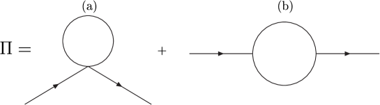
Figure 1: One-loop contributions to the phonon self-energy.

There are two different diagrams that contribute to the one-loop self-energy, see Fig. 1. For external momentum $P=(p_{0},{\bf p})=(i\omega,{\bf p})$, these are

$$\Pi^{(a)}(P)=\frac{\pi^{2}}{27\mu^{4}}\int\frac{d^{d}K}{(2\pi)^{d}}\,\left(2(K\cdot P)^{2}+P^{2}K^{2}\right)S(K)\ ,$$ (11)

and

$$\Pi^{(b)}(P)=\frac{4\pi^{2}}{81\mu^{4}}\int\frac{d^{d}K}{(2\pi)^{d}}\,\Big{(}F(P,K)S(K)S(P-K)\Big{)}\ ,$$ (12)

respectively, where

$$F(P,K)=\left(p_{0}(2K\cdot P-K^{2})+k_{0}(P^{2}-2K\cdot P)\right)^{2}\ .$$ (13)

Above we have used the notational convention of the ITF

$$\int\frac{d^{d}K}{(2\pi)^{d}}\equiv T\sum_{n=-\infty}^{n=\infty}\int\frac{d^{d}k}{(2\pi)^{3}}\ ,$$ (14)

where the sum is over the Matsubara frequencies. We use dimensional regularization to deal with the ultraviolet (UV) divergences of the $T=0$ part of the diagrams, so that $d=3-2\epsilon$. Since the thermal part of the diagrams is UV finite, we will analytically continue back to $d=3$ for their evaluation.

The superfluid phonon is a Goldstone boson, and since thermal effects do not represent an explicit breaking of the $U_{B}(1)$ symmetry, its self-energy should vanish at $P=0$. It is actually easy to check that this holds at one-loop level

$$\Pi^{(a)}(P=0)=\Pi^{(b)}(P=0)=0\ ,$$ (15)

so no thermal mass is generated. This property of the self-energy should hold to all orders in perturbation theory.

After performing the sum over Matsubara frequencies we find that the first diagram only corrects the phonon velocity by a term proportional to $(T/\mu)^{4}\ll 1$.

We proceed with the evaluation of the sum of Matsubara frequencies for the second diagram. We find

$$\Pi^{(b)}(P)=-\frac{4\pi^{2}}{81\mu^{4}}\sum_{s_{1},s_{2}=\pm}\int\frac{d^{d}k}{(2\pi)^{d}}\,F(P,K)\Big{|}_{k_{0}=s_{1}E_{1}}\Big{(}\frac{s_{1}s_{2}}{4E_{1}E_{2}}\frac{1+f(s_{1}E_{1})+f(s_{2}E_{2})}{i\omega-s_{1}E_{1}-s_{2}E_{2}}\Big{)}\ .$$ (16)

where $E_{1}=vk$ and $E_{2}=v|{\bf p-k}|$, and

$$f(x)\equiv\frac{1}{e^{x/T}-1}\ .$$ (17)

After analytical continuation to Minkowski space with retarded boundary conditions, $i\omega\rightarrow p_{0}+i\epsilon$, one notes that this diagram has both real and imaginary parts, the last one being related to the damping of the phonon.

The real part of the diagram gives contributions that behave as follows for low momenta. For $p_{0}=p$, the thermal corrections are proportional to $(T/\mu)^{4}p^{2}$, while the $T=0$ corrections go as $p^{6}/\mu^{4}\ln{(M^{2}/p^{2})}$, where $M$ is a renormalization scale. As for the previous diagram, these corrections are very much suppressed as compared to the tree level physics for $p\ll T\ll\mu$, and we will neglect them.

Although we use the full imaginary part of the self-energy in our computer work, numerically evaluating Eq. (16), we can display an exact analytical limit for illustration. For low external momentum, $p_{0},p\ll T$, we keep only quadratic terms in the external momentum in $F$, so that

$${\rm Im}\,\Pi(p_{0},{\bf p}) \approx \frac{4\pi^{3}}{81\mu^{4}}\int\frac{d^{d}k}{(2\pi)^{d}}\,\frac{E_{1}({\bf k\cdot p})^{2}}{E_{2}}\Big{\{}\left(1+f_{1}+f_{2}\right)\Big{(}\delta(p_{0}-E_{1}-E_{2})$$

$$- \delta(p_{0}+E_{1}+E_{2})\Big{)}-\left(f_{1}-f_{2}\right)\Big{(}\delta(p_{0}-E_{1}+E_{2})-\delta(p_{0}+E_{1}-E_{2})\Big{)}\Big{\}}\ ,$$

where $f_{i}\equiv f(E_{i})$. For $p_{0},p\rightarrow 0$ it is easy to check that the last two delta functions provide the leading order behavior to the integral, so we neglect the first two deltas. For the last two delta functions, we perform the following approximations

$$E_{1}-E_{2}\sim v\,{\bf p\cdot{\hat{k}}}\ ,\qquad f_{1}-f_{2}\sim v\,{\bf p\cdot{\hat{k}}}\frac{df_{1}}{dE_{1}}\ ,$$ (19)

where ${\bf{\hat{k}}}\equiv{\bf k}/k$. Thus, one finds for $d=3$

$${\rm Im}\,\Pi(p_{0},{\bf p})\approx-\frac{2\pi^{3}}{81\mu^{4}}\int_{0}^{\infty}\frac{k^{2}dk}{2\pi^{2}}\,(kp)^{2}\frac{df_{1}}{dE_{1}}\int_{-1}^{1}dx\,x^{3}\Big{(}\delta(x-\frac{p_{0}}{vp})-\delta(x+\frac{p_{0}}{vp})\Big{)}\ ,$$ (20)

and after evaluating the integrals, one gets

$${\rm Im}\,\Pi(p_{0},{\bf p})\approx\frac{8\pi^{5}}{1215}\frac{T^{4}}{v^{7}\mu^{4}}\frac{p^{3}_{0}}{p}\,\Theta(v^{2}p^{2}-p^{2}_{0})\ ,$$ (21)

where $\Theta$ is the step function. This imaginary part of the self-energy corresponds to what is known as Landau damping. Particles disappear or are created through scattering in the thermal bath, and not via the processes which occur at zero temperature.

The damping rate is defined in terms of the on-shell imaginary part of the self-energy

$$\gamma(E_{p})=-\frac{v^{2}}{2E_{p}}\,{\rm Im}\,\Pi(p_{0}=E_{p},{\bf p})\ .$$ (22)

Since we neglect the real corrections to the self-energy, we can take $p_{0}=E_{p}=p/\sqrt{3}$. In the limit $p\rightarrow 0$, we find

$$\gamma=\frac{4\pi^{5}}{405\sqrt{3}}\frac{T^{4}}{\mu^{4}}p+{\cal O}(p^{3})\ .$$ (23)

Let us insist that the $T=0$ contribution to the damping rate is subleading in $p$. The optical theorem indicates that this should be proportional to $\sim p^{5}/\mu^{4}$, as the on-shell imaginary part of the self-energy is related to the square of the tree-level scattering amplitude. Thus, at very low momenta, the thermal damping dominates over the $T=0$ one (but again, we include all effects in our numerical analysis).

Remarkably, we find that the phonons of the CFL and He⁴ superfluids share many properties. They both travel at the speed of sound of the system. Their damping rates for low momenta and at low $T$ follow the same law, going as $\sim pT^{4}$ [22]. Their damping rate at $T=0$ also behaves as $\sim p^{5}$ in both cases [23]. These universal properties are more easily spelled out if one writes an effective field theory for the Goldstone mode of the non-relativistic superfluid [24], where one finds the same sort of cubic and quartic derivative couplings as for the CFL superfluid. This paralellism will be further studied in a separate publication.

4 Phonon mean free path

In this Section we present explicit computations of the mean free path associated to $1\leftrightarrow 2$ and $2\leftrightarrow 2$ phonon collisions. This is a necessary pre-analysis for the study of transport coefficients in the system. In a dilute gas, viscous and other transport coefficients are proportional to the mean free path, and hence inversely proportional to the damping rate or scattering cross section between quasiparticles. Here diluteness implies that the mean flight time between collisions is much larger than the duration of the collision, and in addition Boltzmann’s molecular chaos hypothesis (no correlation between successive collisions) must hold.

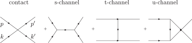
Figure 2: Tree level Feynman diagrams contributing to $2\leftrightarrow 2$ phonon scattering processes.

4.1 Collinear splitting processes

We evaluate the mean free path associated to splitting collinear processes of $1\leftrightarrow 2$ particles. These processes are kinematically forbidden for massive particles, but they are not for massless ones. Because the phonon dispersion relation is linear with Son’s lagrangian, these processes are perfectly collinear, that is, the momenta of the three particles are aligned. Thus, they are not efficient for shear viscosity. They could be efficient if the phonon dispersion law was changed so that the process were not perfectly collinear, but as discussed in Sec. 2, corrections to Son’s lagrangian stemming from higher derivative interaction terms in the effective expansion (suppressed in the $T/\mu$ counting), disallow non-collinear splitting as shown by Zarembo [20].

The inverse of the mean collision time for these processes is obtained averaging the one-loop damping rate computed in Sec. 3. Thus

$$\Gamma_{1\rightarrow 2}=\frac{1}{n}\int\frac{d^{3}p}{(2\pi)^{3}}\,\gamma(E_{p})f(E_{p})\ ,$$ (24)

where

$$n=\int\frac{d^{3}p}{(2\pi)^{3}}\,f(E_{p})=\frac{T^{3}}{4\pi^{2}v^{3}}\zeta(3)\ ,$$ (25)

and $\zeta(x)$ is the Riemann $\zeta$ function with $\zeta(3)=1.202...$.

The mean free path is given by $\lambda=\frac{v}{\Gamma}$. From simple dimensional analysis, it can be inferred that the mean free path for these processes increases at low $T$ as $\mu^{4}/T^{5}$. We have numerically computed $\Gamma$ and the mean free path with the exact one-loop self-energy, checking this power law for low $T$ (see Fig. 3). This may fail at higher $T$ as perturbative corrections to ${\rm Re}\ \Pi$ turn relevant, but that temperature regime is not considered in this article.

4.2 Two-body elastic scattering processes

Here we compute the mean free path of binary collisions, $2\leftrightarrow 2$ processes as depicted in Fig. 2. To evaluate their mean free path one needs the imaginary part of two-loop self-energy diagrams. We employ instead the more direct formulation of kinetic theory, which provides the same answer. Thus, the inverse of the mean collision time is given by

$$\Gamma_{2\to 2}=\frac{v^{2}}{2n}\int_{\bf p,k,p^{\prime},k^{\prime}}f_{\bf p}f_{\bf k}\left(1+f_{\bf p^{\prime}}\right)\left(1+f_{\bf k^{\prime}}\right)(2\pi)^{4}\delta^{(4)}(P+K-P^{\prime}-K^{\prime})\,\arrowvert{\cal T}\arrowvert^{2}\ ,$$ (26)

where

$$\int_{\bf p}\equiv\int\frac{d^{3}p}{2E_{p}(2\pi)^{3}}\ ,$$ (27)

and $\arrowvert{\cal T}\arrowvert^{2}$ is the scattering amplitude squared. We have also used as shorthands $f_{{\bf p}}=f(E_{p})$, etc.

Binary collisions with large or small-angle deflection behave very differently. Let us start with the first ones. Dimensional analysis simply suggests that these proceed with a mean free path of order $\mu^{8}/T^{9}$ [17]. For the typical values of $\mu\sim 500$ MeV and $T\sim 1$ MeV, the mean free path is then larger than $10^{5}$ km, and exceeds the typical radius of a compact star, $R\sim 10$ km. This means that these processes are totally irrelevant for transport phenomena inside the star.

On the other hand, let us consider the $t$-channel scattering in a binary collision, see Fig. 2 (the $u$-channel has the same behavior). It is easy to check that the associated scattering matrix diverges for small-angle collisions. In a massless scalar theory this divergence would be cured through the generation of a thermal mass in the medium, which corrects the low momenta behavior of the propagators. This cannot happen for the phonons defined in Sec. 2, as these particles remain massless at finite $T$. However, the phonon width regulates the divergence, as we detail below.

Let $Q=(\omega,{\bf q})$ be the momentum transfer, $Q=P-P^{\prime}$. Then the scattering matrix in the $t$-channel reads

$$\arrowvert{\cal T}\arrowvert^{2}=\left(\frac{4\pi^{2}}{81\mu^{2}}\right)^{2}\frac{F(P,Q)F(K,-Q)}{\left(\omega^{2}-v^{2}q^{2}\right)^{2}+\left({\rm Im}\,\Pi(\omega,{\bf q})\right)^{2}}$$ (28)

where $F$ was defined in Eq. (13). We have only included the imaginary part of the phonon self-energy, as the real part only gives subleading corrections as already discussed. Were ${\rm Im}\,\Pi=0$, the scattering matrix would diverge when $\omega^{2}\to v^{2}q^{2}$, as the exchanged phonon would be on-shell. This corresponds to a collision where the momenta of the scattered particles is only slightly deflected by the collision. This divergence is regulated by including the damping of the exchanged phonon, which effectively amounts to a resummation of a certain class of diagrams. Because the particles in the thermal bath have typical energies of order $T$, the momentum transfer in the collision will behave typically as $q\ll T$. So for a leading-order estimate of the mean free path, it would suffice to include the value given in Eq. (21), although for numerical computations we can calculate with the full self-energy, and check our approximations.

After regularization, the $2\to 2$ damping rate becomes finite, and dimensional analysis of the mean free path concurs with the full calculation on a $\mu^{4}/T^{5}$ power law (see Appendix A). The numerical estimate (see Fig. 3) teaches us that the mean free path of this process is only slightly smaller than that of the splitting collinear processes.

We have excluded from the analysis the $s$-channel, as it gives a subleading contribution to the mean free path. As opposed to the $t$ and $u$ channels, where the momenta transferred can be arbitrarily small, here it is of order $T$. Thus the regulated divergence in the $s$-channel has much less phase space in the integration region of Eq. (26), and can be safely put aside.

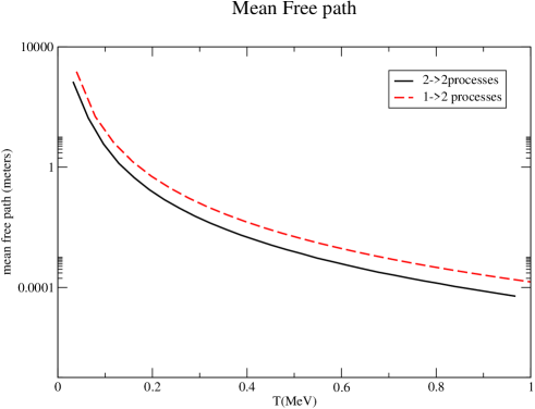
Figure 3: Mean free path below $T=1$ MeV, scaling as $\mu^{4}/T^{5}$. At very low $T$ it exceeds the typical radius of a compact star. A hydrodynamical description in this regime is not meaningful anymore.

Again, we have found the same $T$ dependence for the phonon mean free path as in superfluid Helium below 0.6 K [21]. Initially, Landau and Khalatnikov assumed that the viscosity mean free path was governed by four phonon processes, scaling as $~{}T^{-9}$. Experimental values of the viscosity showed that this was wrong, and that the mean free path was dominated by small-angle collisions, behaving instead as $\sim T^{-5}$, as in the CFL superfluid.

5 Shear viscosity from phonon collisions

In this Section we compute the shear viscosity in the phonon fluid employing kinetic theory. The shear viscosity $\eta$ enters as a dissipative term in the energy-momentum tensor as follows

$$\tau^{ij}=-\eta\left(\partial_{i}V_{j}-\partial_{j}V_{i}-\frac{2}{3}\nabla\cdot{\bf V}\right)\ ,$$ (29)

where ${\bf V}$ is the three dimensional velocity of the phonon fluid in the frame where the superfluid component is at rest. The phonon four velocity is given by $U^{\mu}=(\gamma,-\gamma{\bf V})$, with $\gamma^{-1}=\sqrt{1-V^{2}}$.

The phonon distribution function $f$, under the hypothesis of molecular chaos, obeys the transport equation

$$\frac{df_{{\bf p}}}{dt}=C[f_{{\bf p}}]\ .$$ (30)

In the frame where the superfluid is locally at rest, the Liouville operator appearing in Eq. (30) (and thus the equilibrium solutions) depends on the superfluid velocity Eq. (4). Because we are interested in the shear viscosity of the phonon fluid, and we will linearize the transport equation in gradients of ${\bf V}$, we will neglect the superfluid velocity in all the developments to follow. We note, however, that this approximation would not be valid for the computation of other transport coefficients.

The collision term refers to the binary collisions and splitting/joining processes described in Sec. 4. In the shear viscosity calculation, we neglect the last one for the reasons explained in Sec. 4.1. The binary collision term is given by:

$$C[f_{{\bf p}}]=\frac{1}{2}\int_{\bf k,p^{\prime},k^{\prime}}(2\pi)^{4}\delta^{(4)}(P+K-P^{\prime}-K^{\prime})\,\arrowvert{\cal T}\arrowvert^{2}\frac{1}{2E_{p}}D\ ,$$ (31)

with

$$D=f_{\bf p^{\prime}}f_{\bf k^{\prime}}(1+f_{{\bf p}})(1+f_{\bf k})-f_{{\bf p}}f_{\bf k}(1+f_{\bf p^{\prime}})(1+f_{\bf k^{\prime}})\ .$$ (32)

As usual, the collision term vanishes for the equilibrium distribution $f^{\rm eq.}$, which is given by

$$f^{\rm eq.}_{\bf p}=\frac{1}{e^{P_{\mu}U^{\mu}/T}-1}\ ,$$ (33)

where $P_{\mu}=(E_{p},{\bf p})$.

For the computation of transport coefficients we have to consider small departures from equilibrium so that the distribution function can be written as

$$f=f^{\rm eq.}+\delta f\ .$$ (34)

Accordingly, $D$ can be written as $D=D^{\rm eq.}+\delta D$.

To solve the transport equation we employ the Enskog expansion. To first order we consider the perturbation only on the collision term and linearize it, whereas in the advective term we take the equilibrium distribution function. Since the equilibrium part $f^{\rm eq.}$ annihilates the collision term, we substitute $D$ in Eq. (31) by $\delta D$, that can be written as

$$\delta D=f^{\rm eq.}_{{\bf p}}f^{\rm eq.}_{\bf k}f^{\rm eq.}_{\bf p^{\prime}}f^{\rm eq.}_{\bf k^{\prime}}e^{(E_{p}+E_{k})/T}\Delta[\frac{\delta f}{f^{\rm eq.}}(1-e^{-E/T})]\ ,$$ (35)

where the symbol $\Delta g$ is a shorthand for:

$$\Delta g\equiv g({\bf p^{\prime}})+g({\bf k^{\prime}})-g({\bf p})-g({\bf k})\ .$$ (36)

From the kinetic point of view, the dissipative part of the spatial momentum-stress tensor can be written as:

$$\tau_{ij}=\int\frac{d^{3}p}{(2\pi)^{3}E_{p}}p_{i}p_{j}\,\delta f\ .$$ (37)

To simplify the computations, we assume a velocity profile of the form ${\bf V}=(V_{x}(y),0,0)$. We then assume that the driving shear departures from the equilibrium distribution function can be parameterized as

$$\delta f=-\frac{f^{\rm eq.}}{T}g(p)p_{x}p_{y}\frac{dV_{x}}{dy}\ .$$ (38)

Solving the linearized transport equation for $g(p)$ would yield the shear viscosity, which is expressed as

$$\eta=\frac{4\pi}{15Tv}\int\frac{dp}{(2\pi)^{3}}p^{5}g(p)f^{\rm eq.}\ .$$ (39)

This expression can be viewed as a scalar product

$$\eta=\langle\chi\arrowvert\Phi\rangle$$ (40)

with

$$\chi=p_{i}p_{j}$$ (41)

and $\Phi$ a solution to the Boltzmann equation that can be written as

$$\arrowvert\chi\rangle={C}\arrowvert\Phi\rangle$$ (42)

with $C$ the linearized collision operator. Equivalent to Eq. (40) is then

$$\eta=\langle\Phi\arrowvert C\arrowvert\Phi\rangle$$ (43)

that squared, and substituting (40), yields

$$\eta=\frac{\arrowvert\langle\Phi\arrowvert\chi\rangle\arrowvert^{2}}{\langle\Phi\arrowvert C\arrowvert\Phi\rangle}\ .$$ (44)

In this expression, $\Phi$ is the exact solution of the Boltzmann equation. But it is also amenable to a variational treatment considering a set of test functions $\bar{\Phi}$, where the exact solution $\Phi$ would make (44) reach an extremum (as can be seen by substituting in it $\bar{\Phi}=\Phi+\epsilon$ and observing that the linear terms in $\epsilon$ cancel if $\Phi$ solves the transport equation).

In a rotationally invariant way, we can take the scalar product necessary in these expressions as

$$\cdot=v^{2}\int\frac{d{\bf p}}{E}\frac{f_{0}}{T}\frac{1}{10}\sum_{ij}$$ (45)

and we take as trial function

$$\Phi=g_{ij}(p)=g(p)P_{ij}=g(p)(p_{i}p_{j}-\frac{1}{3}\delta_{ij}p^{2})$$ (46)

$$g(p)=\frac{p^{\nu}}{1-e^{-E_{p}/T}}$$

with $\nu$ a variational parameter. This family is general enough to allow treatment of a polynomial family such as used in [28], but also includes rational functions. For this family, Eq. (44) reduces to

$$\eta[\nu]=\frac{(I[\nu])^{2}}{L[\nu]}\ ,$$ (47)

with

$$I[\nu]=\frac{v^{2}}{15}\int\frac{dp}{E}p^{4}\frac{f^{\rm eq.}}{T}\frac{p^{\nu}}{1-e^{-E_{p}/T}}\ ,$$ (48)

and

$$L[\nu]=\frac{1}{40T}\int_{\bf p,k,p^{\prime},k^{\prime}}(2\pi)^{4}\delta^{4}(P+K-P^{\prime}-K^{\prime})\frac{\arrowvert T\arrowvert^{2}}{2}$$ (49)

$$e^{(E_{p}+E_{k})/T}f^{\rm eq.}_{\bf p}f^{\rm eq.}_{\bf k}f^{\rm eq.}_{\bf p^{\prime}}f^{\rm eq.}_{\bf k^{\prime}}\Delta(P_{ij}p^{\nu})\Delta(P_{ij}p^{\nu})\ .$$

As the integrand of $L[\nu]$ is positive definite, so is also Eq. (47). The computation of $I[\nu]$ is easy, but to compute $L[\nu]$ requires a multidimensional Montecarlo integration. This is quite a technical calculation and is detailed in the Appendices, but we will point out some subtleties here.

It is worth stressing that for a quick order of magnitude estimate of the shear viscosity, it is usually correct to pick up as a trial function the case considered for $\nu=0$. It usually gives also the correct parametric behavior of the viscosity. However, in this case this is not so, as some values of the parameter $\nu$ cause a zero-mode in the collision term. We have identified two of these zero-modes.

Let us first see why these zero modes occur. For a general trial function, the denominator of Eq. (47), and as explained at length in the previous sections, is dominated by contributions to the integral coming from (almost) collinear collisions due to the divergence in the naked $t$-channel amplitude. This divergence is however regulated by the inclusion of Landau damping, see Eq. (28). For a perfect collinear collision, the conservation of energy momentum at the vertex $\delta^{(3)}({\bf k}+{\bf q}-{\bf p})\delta(E_{k}+\omega-E_{p})$, where $\omega$ and ${\bf q}$ are the energy and momentum transfer, together with $E_{p}=vp$ requires that ${\bf p}$, ${\bf k}$ and ${\bf q}$ are all parallel. Therefore all entering and outgoing boson momenta in a collinear collision are parallel. However, in solving the transport equation, a special choice of trial wavefunction may force a zero in this collinear limit and it can thus achieve a cancellation. Then this zero mode dominates the inversion of the collision operator $C$ when solving the Boltzmann equation.

This property of the (linearized) collision operator stems from the term

$$\sum_{ij}\Delta(P_{ij}p^{\nu})\Delta(P_{ij}p^{\nu})\ .$$ (50)

Now observe the cancellation for $\nu=-2$. In this case, $P_{ij}p^{-2}=\hat{p}_{i}\hat{p}_{j}-\frac{\delta_{ij}}{3}$ depends only on the unit vector along the momentum, and

$$\Delta(P_{ij}p^{\nu})=\hat{p}_{i}\hat{p}_{j}+\hat{k}_{i}\hat{k}_{j}-\hat{p^{\prime}}_{i}\hat{p^{\prime}}_{j}-\hat{k^{\prime}}_{i}\hat{k^{\prime}}_{j}=0\ .$$ (51)

for a perfect collinear collision. A second zero-mode is given by the variational value $\nu=-1$. Then

$$\Delta(P_{ij}p^{\nu})=\frac{1}{v}\left(\frac{}{}E_{p}\hat{p}_{i}\hat{p}_{j}+E_{k}\hat{k}_{i}\hat{k}_{j}-E_{p^{\prime}}\hat{p^{\prime}}_{i}\hat{p^{\prime}}_{j}-E_{k^{\prime}}\hat{k^{\prime}}_{i}\hat{k^{\prime}}_{j}+\frac{1}{3}\delta_{ij}(E_{p}+E_{k}-E_{p^{\prime}}-E_{k^{\prime}})\right).$$ (52)

This also vanishes in the collinear limit upon employing the energy-conservation equation.

The collision operator does not vanish because contributions to the integral not in the perfect collinear limit still provide a contribution, and thus a near-zero mode, not an exact zero mode, appears.

We have carried out a variational study of $\eta[\nu]$ numerically (see Appendix B), and we have reached to the conclusion that $\eta$ is maximized for the value $\nu=-1$, which corresponds to one of the (near) zero-modes explained above.

We quote here the final outcome of these analysis. Due to the existence of the (near) zero mode with $\nu=-1$ that suppresses collinear scattering, all $2\leftrightarrow 2$ channels are included, and the viscosity behaves as

$$\eta=1.3\!\cdot\!10^{-4}\!\cdot\!\frac{\mu^{8}}{T^{5}}\ {\rm MeV}^{3}\ .$$ (53)

For illustration we also give the result for low momentum transfer that is amenable to analytical treatment when only the $t$-channel is included the viscosity behaves instead as

$$\eta\sim 4\!\cdot\!10^{12}\!\cdot\!\frac{\mu^{8}}{T^{5}\log{|T/\mu|}}\,{\rm MeV}^{3}\ .$$ (54)

6 Contribution of the in-medium electromagnetism to the viscosity

In considering transport coefficients for the CFL quark star we should examine the contribution of the in-medium electromagnetism, since the very light electron could conceivably transport momentum efficiently. The effective coupling of the in-medium photon and the electron is ${\widetilde{e}}=e\cos{\theta}$, where $e$ is the electromagnetic coupling constant, and the mixing angle is [29]

$$\cos{\theta}=\frac{\sqrt{3}g}{\sqrt{3g^{2}+4e^{2}}}\ ,$$ (55)

CFL quark matter is a dielectric at low energies, with dielectric constant [29]

$$\widetilde{\epsilon}=1+\frac{{2\,}}{9\pi^{2}}\frac{\widetilde{e}^{2}\mu^{2}}{\Delta^{2}}\ .$$ (56)

In particular, this implies that the in-medium photon travels at a speed ${\widetilde{v}}_{\gamma}=1/\sqrt{\widetilde{\epsilon}}$, less than the speed of light. Reflection and refraction properties of light on CFL quark matter have been studied in [30].

The value of the shear viscosity can be borrowed from QED, by taking into account the following replacements in the electromagnetic fine structure constant

$$\alpha\rightarrow{\widetilde{\alpha}}=\frac{{\widetilde{e}}^{2}}{4\pi\sqrt{\widetilde{\epsilon}}}=\alpha\frac{\cos^{2}{\theta}}{\sqrt{\widetilde{\epsilon}}}$$ (57)

Transport properties in a photon-electron system in the regime $T<m_{e}$, where $m_{e}=0.5$ MeV is the electron mass, have been computed in [31]. While the computation, based on electron-in medium photon scattering at an arbitrary temperature can only be done numerically, approximate analytical results give

$$\eta^{\rm e.m.}=\frac{20x_{\gamma}}{27x_{e}}\frac{T}{\sigma_{T}}\ ,$$ (58)

where $\sigma_{T}$ is the Thomson cross-section

$$\sigma_{T}=\frac{8}{3}\pi\left(\frac{{\widetilde{\alpha}}}{m_{e}}\right)^{2}\ ,$$ (59)

and $x_{\gamma,e}=n_{\gamma,e}/(n_{\gamma}+n_{e})$ measures the relative concentrations of photons/electrons.

For an order of magnitude estimate, one can take ${\widetilde{\alpha}}\sim 1/137$, as for moderates densities ${\widetilde{\epsilon}}$ never becomes too large. Then, one can see that the electromagnetic contribution to the shear viscosity is negligible compared to the phonon contribution at temperatures of order $0.1$ MeV. Further lowering the temperature makes Eq. (58) increase rapidly because of the Boltzmann density factor $e^{-m/T}$ in the denominator containing the electron density. However, light by light scattering processes come to play (these can be treated with the Euler-Heisenberg effective lagrangian as reviewed in [32]) and the photon scattering cross section is not exponentially low.

7 Further improvements

Let us comment on possible corrections to our results. First, one could better determine the self-interactions of the phonons. According to ref. [19], corrections to the effective Lagrangian Eq. (8) can be obtained with a better determination of the EOS of CFL quark matter. Nevertheless, as the EOS is dominated by a term going as $\sim\mu^{4}$, corrections to the phonon Lagrangian will not modify the leading parametric dependence on $\mu$ of the three-phonon vertex, the relevant one for transport in the superfluid, and would only alter the numerical factor in front of this term in the effective Lagrangian.

Second, one could better determine the collision term entering the transport equation. We saw that Landau damping regulates an otherwise divergent scattering matrix of binary collisions (see Sec. 3). Taking into account the width of the exchanged phonon amounts to a resummation of diagrams, where multiple splitting/joining scatterings are treated as independent classical events. Since the mean free path associated to the $2\leftrightarrow 2$ and the $1\leftrightarrow 2$ collisions are of the same order, this approximation is not quite correct. One should take into account the Landau-Pomeranchuk-Migdal (LPM) effect, which would better determine the collision term [33, 34, 35]. This correction would not modify the parametric behavior of $\eta$, but would again affect the preceding numerical factor.

One should as well be concerned about possible changes in the shear viscosity when either higher derivative interactions or higher order corrections are included in the phonon dispersion relation. As already discussed in Sec. 2, Zarembo [20] has shown that to all orders in $\frac{\Delta}{\mu}$, the interaction terms are suppressed by powers of $\mu$, not $\Delta$. Also of interest to us is Zarembo’s observation that the phonon dispersion relation is given by Eq. (9). As $k$ is increased, the phonons move slower. The negative coefficient in the correction to the linear law above reveals that corrections to the dispersion relation beyond Son’s theory suppress collinear splitting (a phonon cannot decay into two phonons of larger joint energy at $T=0$). Therefore we are safe in ignoring the $1\to 2$ processes in our computation of the shear viscosity.

We note that for superfluid He⁴, the phonon dispersion relation used in ref. [21] to match the experimental value of the shear viscosity is of the form

$$\omega_{s}(k)=vk\left[1+g(k)\right]\ .$$ (60)

with $g(k)$ a positive function that tends to zero for $k\rightarrow 0$. In this way, phonons with high momenta move faster than those of low momenta and can decay into two slower phonons. Maris used the experimental value of the viscosity to gain information about the function $g(k)$. It then turns out that in superfluid He⁴ almost collinear processes are more relevant than large-angle collisions for the shear viscosity at very low temperature.

For astrophysical applications an order of magnitude estimate for the values of the viscosities is good enough to study properties of compact stars. Other transport properties would also be needed, but they will be the subject of a different project.

8 Discussion

We finally summarize our main findings and conclusions. CFL quark matter at very low $T$ behaves as a superfluid of the sort He⁴, rather than of the sort of He³, as wrongly assumed in the literature. Dissipative processes in such a cold regime are dominated by phonon-phonon scattering. This analogy is reflected in $T$-power laws for the thermal properties of phonons of the CFL and He⁴ superfluids.

For astrophysical applications, we should emphasize the following. At sufficiently low $T$ the phonon mean free path would exceed the radius of a compact star. We can give a crude estimate of the temperature when this will occur, simply by considering the equation

$$R<L\sim\mu^{4}/T^{5}\ .$$ (61)

If the quark chemical potential is of order $\mu\sim 500$ MeV, and we consider $R\sim 10$ km, we find that for $T<0.06$ MeV superfluid phonons do not scatter within the star. Transport coefficients could then be dominated by the tiny contribution of the in-medium electromagnetism, but an evaluation of the photon mean free path also shows that for $T\sim 0.02$ MeV it also exceeds the radius of the star [18]. Below that temperature, CFL quark matter in the star would behave as a perfect superfluid, as a hydrodynamical description of the phonon and electron fluids would be meaningless. The superfluid hydrodynamical equations would then be given by Eqs. (3) and (5), showing then no dissipation.

In a rotating superfluid there are vortices. To study the rotational properties of a hypothetical CFL quark star, one cannot obviate that fact. In view of our results, the analysis of r-mode instabilities of a CFL quark star should then be redone, taking into account both the temperature regime of the star, and the vortex dynamics of the CFL phase. The bulk viscosity should also be needed, but we leave this computation for a different project.

Appendix A Evaluation of the $2\to 2$ processes

In this Appendix we give some details on the Montecarlo numerical evaluations of the multiple integrals appearing in two-body elastic scattering. Here we treat Eq. (26) at length. The integral is dominated by t-channel scattering (the u-channel contribution is equal and amounts to a factor 2) due to the collinear singularity. Then for production runs it is sufficient to maintain the $t$-channel scattering matrix $\arrowvert{\cal T}\arrowvert^{2}$ and neglect the rest of the interaction diagrams. The numerator of Eq. (26) has twelve integrations. Three, for example over ${\bf k^{\prime}}$, can be immediately performed with the help of the three-momentum $\delta$ in Eq. (26). We choose for the nine remaining integrals the incoming three-momenta $\bf p$, $\bf k$, and the transferred momentum ${\bf q}={\bf p}-{\bf p^{\prime}}={\bf k^{\prime}}-{\bf k}$.

Our freedom to choose the third axis makes the angular integrals around $\bf q$ to be $4\pi$. Since we approximate the integral to be dominated by $t$-channel exchange, the scattering matrix element $\arrowvert{\cal T}\arrowvert^{2}$ can only depend on the two polar angles (through the derivative coupling in the vertex), $\hat{\bf p}\!\cdot\!\hat{\bf q}$ and $\hat{\bf k}\!\cdot\!\hat{\bf q}$ and not on the azimuthal angles $\phi_{\bf p}$ and $\phi_{\bf k}$. Therefore the latter are also trivial.

Introduction of an auxiliary variable $\omega$ (energy transfer) allows to write the energy $\delta$ in Eq. (26) as

$$\delta(E_{k}+E_{p}-E_{k^{\prime}}-E_{p^{\prime}})=\int_{-\infty}^{+\infty}d\omega\,\delta(w-E_{p}+E_{p^{\prime}})\delta(\omega+E_{k}-E_{k^{\prime}})\ .$$ (62)

Then it is easy to employ the resulting two $\delta$ functions to compute the remaining polar angular integrals. In exchange, the integral over the auxiliary variable remains. With these manipulations we obtain

$$\Gamma(T)=\frac{1}{vT^{3}\pi^{3}\varsigma(3)2^{8}}\int_{0}^{\infty}dq\int_{-vq}^{vq}d\omega\int_{\frac{vq-\omega}{2v}}^{\infty}dk\int_{\frac{vq+\omega}{2v}}^{-\infty}dpf_{{\bf p}}f_{\bf k}(1+f_{\bf k^{\prime}})(1+f_{\bf p^{\prime}})\arrowvert{\cal T}\arrowvert^{2}\ ,$$ (63)

where $\arrowvert{\cal T}\arrowvert^{2}$ is given in Eq. (28). This is an integral in four dimensions dominated by the region around the on-shell singularities for $\omega\simeq vq$ and $\omega\simeq-vq$. To obtain good numerical convergence these singularities, which are regulated by Landau damping, need to be isolated. First, perform one more change of variables to

$$x=\omega+vq\ ;\ \ y=\omega-vq\ .$$ (64)

The integrals over $x$ and $y$ run from $0$ to $\infty$ and from $-\infty$ to $0$ respectively. The on-shell singularities occur now at $x=0$, $y=0$. Therefore we introduce a low momentum cut-off on these variables, $\lambda$, that serves to split the regions of integration in the $xy$ plane as (1) $(0,\lambda)\times(-\lambda,0)$; (2) $(0,\lambda)\times(-\infty,-\lambda)$; (3) $(\lambda,\infty)\times(-\lambda,0)$; (4) $(\lambda,\infty)\times(-\infty,-\lambda)$. The value of the integral should of course be independent of the value of $\lambda$ since this merely splits the integration region. Choosing $\lambda\ll T$ allows to evaluate most of the integrand in regions (2) and (3) at $x=0\ ,y=0$ respectively, and therefore the $x$ ($y$) integral can be performed analytically. Explicit numerical evaluation shows that regions (1) and (4) are negligible with respect to the contributions from regions (2) and (3) whenever $\lambda$ is large compared to $\frac{{\rm Im}\Pi\arrowvert_{y=0}}{x}$ (or the same expression reversing $x$ and $y$). Under these conditions we need to concentrate only on regions (2) and (3).

For region (3) the relevant $y$ integral is

$$I\approx F(P,x,y=0)\int_{-\lambda}^{0}dy\frac{1}{x^{2}y^{2}+({\rm Im}\Pi(x,y=0))^{2}}\ .$$ (65)

Since in this region $x>\lambda$, the imaginary part takes a constant value as $y\to 0$. Therefore the integral is regulated and yields an arctangent. All the derivative couplings and Bose-Einstein factors are smooth at $y=0$ and have been pulled out of the integral as a constant (still function of $x$) $F(P,x,y=0)$, since the interval is small respect to $T$. Therefore

$$I=F(P,x,y=0)\approx\frac{\pi/2}{x\,{\rm Im}\Pi(x,y=0)}\ .$$ (66)

Finally the damping rate can be given to very good accuracy in terms of three quadratures

$$\Gamma = \frac{1}{128\varsigma(3)v^{2}T^{3}}\frac{\pi}{(81\mu^{4})^{2}}\left(\bar{\Gamma}_{2}+\bar{\Gamma}_{3}\right)$$ (67)

$$\Gamma_{2} \simeq \int_{-\infty}^{-\lambda}dy\int_{-y/2v}^{\infty}dk\int_{0}^{\infty}dpf_{{\bf p}}f_{\bf k}(1+f_{\bf k^{\prime}})(1+f_{\bf p^{\prime}})\frac{\pi/2}{y\,{\rm Im}\Pi(x=0,y)}\left(F(P,-Q)F(K,Q)\right)\arrowvert_{x=0}$$

$$\Gamma_{3} \simeq \int_{\lambda}^{\infty}dx\int_{x/2v}^{\infty}dp\int_{0}^{\infty}dkf_{{\bf p}}f_{\bf k}(1+f_{\bf k^{\prime}})(1+f_{\bf p^{\prime}})\frac{\pi/2}{x\,{\rm Im}\Pi(x,y=0)}\left(F(P,-Q)F(K,Q)\right)\arrowvert_{y=0}\ .$$

The remaining three integrals are routinely calculated with a computer code and yield the damping rate. Evaluation of the shear viscosity is dealt with in the next two sections.

Appendix B Numerical evaluation of shear viscosity

Table 1: Numerical cancellation of the internal $\lambda$ dependence in $\eta(-2)$ given by eq. (47) employing the zero mode trial wavefunction $\nu=-2$. The temperature is $T=0.001$ MeV, the cutoff for external momenta is $\Lambda=100T$ and the cutoff over the $x$, $y$ integrations is $0.6\Lambda$, large enough to cover all relevant phase space but small enough to avoid the Montecarlo points to be dispersed where the Bose-Einstein factor damps the integrand. The calculation is performed with 256000 points in each integration domain, doubled four times for convergence, and the integral is computed ten times for each fixed number of points. The standard deviation obtained is 1% . A small logarithmic drift of the result is still observed, but this is now of the order of the uncertainty in the Montecarlo and not very relevant. A meaningful cutoff $\lambda$ needs to be smaller than $T$ but of a similar order of magnitude.

$\lambda$	$\eta(\nu=-2)(MeV^{3})$
$T/12$	$1.09\!\cdot\!10^{33}$
$T/25$	$1.10\!\cdot\!10^{33}$
$T/50$	$1.12\!\cdot\!10^{33}$
$T/100$	$1.14\!\cdot\!10^{33}$
$T/200$	$1.16\!\cdot\!10^{33}$

Our Montecarlo program, employing the subroutine Vegas [36] has been written in two versions. One perfoms three and four dimensional integrals keeping only the t-channel exchange contribution to the cross section as previously described, and is useful to isolate this precisely. If other scattering processes also contribute, this program cannot be used since two azimutal angles are now not trivial. In this case a second version performs the five dimensional integral over all phase space and is a generic purpose integrator (but diluting the available computing power over a larger region makes it less precise to capture t-channel singularities). In table 2 where we present various numerical results, these two versions are denoted as (t-channel) and (all) respectively.

Table 2: Numerical output of our programs for shear viscosity. The program marked (t-channel) ignores contributions from s-channel exchange and contact terms, as well as crossed terms between them when evaluating $\arrowvert T\arrowvert^{2}$. Therefore it evaluates only three and four-dimensional integrals as opposed to (all) that performs five-dimensional integration. The cutoff for external momenta is $100T$, the cutoff for transferred $q$, $\omega$ is $60T$, and for the (t-channel) version, the infrared separation for the very nearly collinear zone is at $\lambda=T/100$. All units are $MeV$.

$T$	Variational parameter $\nu$	$\eta$ (t-channel)	$\eta$ (all)
$10^{-3}$	$-3$	$9.7\!\cdot\!10^{12}$	$2.3\!\cdot\!10^{31}$
$10^{-3}$	$-2$	$1.1\!\cdot\!10^{33}$	$1.3\!\cdot\!10^{32}$
$10^{-3}$	$-1$	$1.1\!\cdot\!10^{48}$	${\bf 5.0\!\cdot\!10^{32}}$
$10^{-3}$	$0$	$4.8\!\cdot\!10^{13}$	$1.6\!\cdot\!10^{30}$
$10^{-3}$	$1$	$2.9\!\cdot\!10^{12}$	$8.6\!\cdot\!10^{28}$
$10^{-3}$	$1$	$3.6\!\cdot\!10^{11}$	$9.9\!\cdot\!10^{27}$
$10^{-2}$	$-3$	$1.0\!\cdot\!10^{12}$	$2.3\!\cdot\!10^{26}$
$10^{-2}$	$-2$	$1.4\!\cdot\!10^{28}$	$1.3\!\cdot\!10^{27}$
$10^{-2}$	$-1$	$1.4\!\cdot\!10^{43}$	${\bf 5.0\!\cdot\!10^{27}}$
$10^{-2}$	$0$	$4.8\!\cdot\!10^{12}$	$1.6\!\cdot\!10^{25}$
$10^{-2}$	$1$	$2.9\!\cdot\!10^{11}$	$8.6\!\cdot\!10^{23}$
$10^{-2}$	$2$	$3.6\!\cdot\!10^{10}$	$9.9\!\cdot\!10^{22}$
$10^{-1}$	$-3$	$1.1\!\cdot\!10^{11}$	$2.3\!\cdot\!10^{21}$
$10^{-1}$	$-2$	$2.6\!\cdot\!10^{23}$	$1.3\!\cdot\!10^{22}$
$10^{-1}$	$-1$	$1.9\!\cdot\!10^{38}$	${\bf 5.0\!\cdot\!10^{22}}$
$10^{-1}$	$0$	$4.8\!\cdot\!10^{11}$	$1.6\!\cdot\!10^{20}$
$10^{-1}$	$1$	$2.9\!\cdot\!10^{10}$	$8.6\!\cdot\!10^{18}$
$10^{-1}$	$2$	$3.6\!\cdot\!10^{9}$	$9.9\!\cdot\!10^{17}$

The numerical results from our Montecarlo for the shear viscosity are given in full in table 2. The variational calculation is somewhat complex and care needs to be exercised upon its interpretation. In this table, the first column gives the temperature in MeV. The second is the variational parameter $\nu$ that varies from a strong infrared enhancement to polynomial suppression. The fourth column displays the values obtained for the viscosity with all interactions included. These are extracted in the third column.

The fourth column displays very clearly the $\frac{\mu^{8}}{T^{5}}$ behaviour characteristic of the naive power counting. However, for a general $\nu$, one should go to the result of the t-channel exchange. For example, for $\nu=0$ that corresponds to the usual zero’th order approximation in a polynomial expansion, and at $T=0.1$ MeV, the viscosity would behave as $\eta\simeq 0.8\!\cdot\!\frac{\mu^{4}}{T}$.

But this conclusion would miss the effects of the zero mode. By studying $\eta(\nu)$ with the t-channel calculation (again the third column, at fixed $T$), one observes that the zero modes discussed above corresponding to $\nu=-2$ and $\nu=-1$ yield variational maxima, especially $\nu=-1$, a mildly dependent on the numerical grid and cutoffs. The analytical considerations suggest a logarithmic dependence, as discussed in the main text.

Finally a glance at the fourth column reveals that this formula is much larger (and therefore the integral (49) very suppressed) than the corresponding naive counting for this value of the variational parameter. This entry also happens to be the maximum of the third column, finally concluding that the viscosity must behave in this temperature range as in Eq.(53). The plot 4 enlightens this discussion by showing how the t-channel contribution is much lower than the corresponding $T^{-5}$ behaviour for $\nu=-1$, $\nu=-2$.

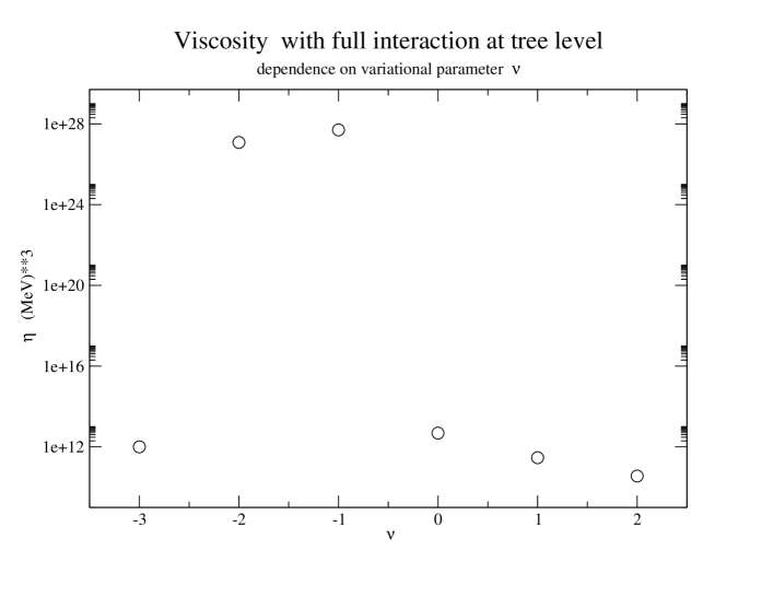
Figure 4: The variational evaluation including boson exchanges in the interaction shows a maximum corresponding to the zero modes that make the t-channel contribution suppressed. The maximum within the functional family $\frac{p^{\nu}}{1-e^{-E_{p}/T}}$ corresponds to $\nu=-1$. The Temperature is fixed at 0.01 $MeV$.

References

- [1] D. Bailin and A. Love, Phys. Rept. 107, 325 (1984).
- [2] K. Rajagopal and F. Wilczek, hep-ph/0011333.
- [3] M. G. Alford, Ann. Rev. Nucl. Part. Sci. 51 (2001) 131 [arXiv:hep-ph/0102047].
- [4] M. Alford, K. Rajagopal and F. Wilczek, Nucl. Phys. B 537, 443 (1999). [arXiv:hep-ph/9804403].
- [5] N. Andersson, Astrophys. J. 502, 708 (1998) [arXiv:gr-qc/9706075].
- [6] J. Madsen, Phys. Rev. D 46 (1992) 3290.
- [7] J. Madsen, Phys. Rev. Lett. 85, 10 (2000) [arXiv:astro-ph/9912418].
- [8] K. Rajagopal and F. Wilczek, Phys. Rev. Lett. 86, 3492 (2001) [arXiv:hep-ph/0012039].
- [9] S. Reddy, M. Sadzikowski and M. Tachibana, Nucl. Phys. A 714, 337 (2003) [arXiv:nucl-th/0203011].
- [10] P. Jaikumar, M. Prakash and T. Schafer, Phys. Rev. D 66, 063003 (2002) [arXiv:astro-ph/0203088].
- [11] R. Casalbuoni and R. Gatto, Phys. Lett. B464 (1999) 111 [arXiv:hep-ph/9908227].
- [12] D. T. Son and M. A. Stephanov, Phys. Rev. D61, 074012 (2000) [arXiv:hep-ph/9910491]; Phys. Rev. D62, 059902 (2000) [arXiv:hep-ph/0004095].
- [13] P. F. Bedaque and T. Schafer, Nucl. Phys. A 697, 802 (2002) [arXiv:hep-ph/0105150].
- [14] D. B. Kaplan and S. Reddy, Phys. Rev. D 65, 054042 (2002) [arXiv:hep-ph/0107265].
- [15] C. Manuel and M. H. Tytgat, Phys. Lett. B479, 190 (2000) [arXiv:hep-ph/0001095].
- [16] T. Schafer, Phys. Rev. D 65, 094033 (2002) [arXiv:hep-ph/0201189].
- [17] I. A. Shovkovy and P. J. Ellis, Phys. Rev. C 66, 015802 (2002) [arXiv:hep-ph/0204132].
- [18] I. A. Shovkovy and P. J. Ellis, Phys. Rev. C 67, 048801 (2003) [arXiv:hep-ph/0211049].
- [19] D. T. Son, arXiv:hep-ph/0204199.
- [20] K. Zarembo, Phys. Rev. D 62, 054003 (2000) [arXiv:hep-ph/0002123].
- [21] H. J. Maris, Phys. Rev. A 8, 1980 (1973).
- [22] P. C. Hohenberg and P. C. Martin, Ann. Phys. (N.Y.) 34, 291 (1965).
- [23] S. T. Beliaev, Sov. J. Phys. 7, 289 (1958); 34, 299 (1958).
- [24] J. O. Andersen, arXiv:cond-mat/0209243.
- [25] L. Landau and Lifschitz, “Statistical Physics” vol. 5;“Fluid Mechanics” vol. 6, Prentince Hall, New Jersey.
- [26] V. V. Lebedev and I. M. Khalatnikov, Zh. Eksp. Teor. Fiz. 56, 1601 (1982); B. Carter and I. M. Khalatnikov, Rev. Math. Phys. 6, 277 (1994)
- [27] D. T. Son, unpublished and private communication.
- [28] A. Dobado and F. J. Llanes-Estrada, arXiv:hep-ph/0309324.
- [29] D. F. Litim and C. Manuel, Phys. Rev. D 64, 094013 (2001) [arXiv:hep-ph/0105165].
- [30] C. Manuel and K. Rajagopal, Phys. Rev. Lett. 88, 042003 (2002) [arXiv:hep-ph/0107211].
- [31] S. R. de Groot, W. A. Van Leeuwen and Ch. van Weert, “Relativistic Kinetic Theory”, North-Holland, Amsterdam, 1980.
- [32] A. Dobado et al, Effective lagrangians for the Standard Model, Springer Verlag, Berlin-Heidelberg 1997.
- [33] L. D. Landau and I. Pomeranchuk, Dokl. Akad. Nauk Ser. Fiz. 92, 735 (1953).
- [34] L. D. Landau and I. Pomeranchuk, Pair Dokl. Akad. Nauk Ser. Fiz. 92, 535 (1953).
- [35] P. Arnold, G. D. Moore and L. G. Yaffe, JHEP 0301, 030 (2003) [arXiv:hep-ph/0209353].
- [36] G. P. Lepage, CLNS-80/447