TUM-HEP-549/04

hep-ph/0406048

Early $SU(4)_{\rm PS}\otimes SU(2)_{L}\otimes SU(2)_{R}\otimes SU(2)_{H}$

Unification of Quarks and Leptons

Andrzej J. Buras,^a P.Q. Hung,^b Ngoc-Khanh Tran,^b Anton Poschenrieder^a and Elmar Wyszomirski^a

^a Physik Department, Technische Universität München, D-85748 Garching, Germany

^b Dept. of Physics, University of Virginia, 382 McCormick Road
P. O. Box 400714, Charlottesville, Virginia 22904-4714, USA

We discuss various aspects of the early petite unification (PUT) of quarks and leptons based on the gauge group $G_{\rm PUT}=SU(4)_{\rm PS}\otimes SU(2)_{L}\otimes SU(2)_{R}\otimes SU(2)_{H}$. This unification takes place at the scale $M={\cal O}(1-2~{}{\rm TeV})$ and gives the correct value of $\sin^{2}\theta_{W}(M_{Z}^{2})$ without the violation of the upper bound on the $K_{L}\to\mu e$ rate and the limits on FCNC processes. These properties require the existence of three new generations of unconventional quarks and leptons with charges up to $4/3$ (for quarks) and 2 (for leptons) and masses ${\cal O}(250\,{\rm GeV})$ in addition to the standard three generations of quarks and leptons. The horizontal group $SU(2)_{H}$ connects the standard fermions with the unconventional ones. We work out the spontaneous symmetry breaking (SSB) of the gauge group $G_{\rm PUT}$ down to the SM gauge group, generalize the existing one-loop renormalization group (RG) analysis to the two-loop level including the contributions of Higgs scalars and Yukawa couplings, and demonstrate that the presence of three new generations of heavy unconventional quarks and leptons with masses ${\cal O}(250\,{\rm GeV})$ is consistent with astrophysical constraints. The NLO and Higgs contributions to the RG analysis are significant while the Yukawa contributions can be neglected.

1 Introduction

The idea of Grand Unification (GUT) based on simple groups like SU(5) [1, 2] or SO(10) [3, 4], characterized by a single gauge coupling $g_{\rm GUT}$, is a very attractive scenario of the physics beyond the Standard Model (SM). In GUT models quarks and leptons are generally members of the same representation under the given gauge group, and this results in transitions that violate quark and lepton quantum numbers. As such transitions are very suppressed in nature, the GUT scale must be very large, typically ${\cal O}(10^{16}\,{\rm GeV})$, in order to be consistent with the experimental data, in particular with the lower bound on the proton life-time.

A less ambitious program is the Petite Unification [5, 6] that aims at unifying quarks and leptons at some energy scale $M$, not much greater than the electroweak scale, with the gauge group $G_{S}\otimes G_{W}$ that is characterized by two independent couplings $g_{S}$ and $g_{W}$. It is further assumed that $G_{S}$ and $G_{W}$ are either simple or pseudosimple (a direct product of simple groups with identical couplings). An attractive choice for the strong group $G_{S}$ is $SU(4)$ a la Pati-Salam [7] with the lepton number playing the role of the fourth colour. It turns out [6] that with this choice of $G_{S}$ only very few weak groups $G_{W}$ can have low unification scale being simultaneously consistent with the measured value of $\sin^{2}\theta_{W}(M_{Z}^{2})$, the upper bound on the rare decay $K_{L}\to\mu e$ and the data on flavour changing neutral current (FCNC) processes. Basically only two weak gauge groups $SU(2)^{3}$ and $SU(3)^{2}$ can be made consistent with the experimental data.

The general properties of the $SU(4)_{\rm PS}\otimes SU(2)^{3}$ and $SU(4)_{\rm PS}\otimes SU(3)^{2}$ unifications have been discussed in [6]. In these models the values of $\sin^{2}\theta_{W}$ at the unification scale $M$ turn out to be $1/3$ and $3/8$, but a very fast renormalization group evolution allows to obtain correct $\sin^{2}\theta_{W}(M_{Z}^{2})$ with $M\approx 1~{}{\rm TeV}$ and $M\approx 3~{}{\rm TeV}$, respectively.

Concentrating on the unification based on the gauge group

$$G_{\rm PUT}=SU(4)_{\rm PS}\otimes SU(2)_{L}\otimes SU(2)_{R}\otimes SU(2)_{H},$$ (1.1)

let us recall three most interesting properties of this model:

• In addition to the standard three generations of quarks and leptons, new three generations of unconventional quarks and leptons with charges up to $4/3$ (for quarks) and 2 (for leptons) and masses ${\cal O}(250\,{\rm GeV})$ are automatically present. The horizontal group $SU(2)_{H}$ connects the standard fermions with the unconventional ones.

• The placement of the ordinary quarks and leptons in the fundamental representation of $SU(4)_{\rm PS}$ is such that there are no tree-level transitions between ordinary quarks and leptons mediated by the $SU(4)_{\rm PS}$ gauge bosons. This prevents rare decays such as $K_{L}\rightarrow\mu e$ from acquiring large rates, even when the masses of these gauge bosons are in the few TeV’s range.

• There are new contributions to flavour changing neutral current processes (FCNC) involving standard quarks and leptons that are mediated by the horizontal $SU(2)_{H}$ weak gauge bosons and the new unconventional quarks and leptons. However, they appear first at the one–loop level and can be made consistent with the existing experimental bounds.

It should be emphasized that the existence of new heavy fermions that are placed in the fundamental representation of $SU(4)_{\rm PS}$ together with ordinary fermions is essential for having early unification of quarks and leptons without the problems with the rare decays like $K_{L}\rightarrow\mu e$. The original petite unification group $SU(4)_{\rm PS}\otimes SU(2)^{4}$ [5] having only ordinary fermions in the fundamental representation of $SU(4)_{\rm PS}$ and consequently $K_{L}\rightarrow\mu e$ proceeding at the tree level is ruled out as the early unification model unless further new physics, such as large extra dimensions, is invoked [8]. In comparison with the usual left–right symmetric models based on the $SU(4)_{\rm PS}\otimes SU(2)_{L}\otimes SU(2)_{R}$ group [9, 10], that is relevant for the grand $SO(10)$ unification, the present model has an additional $SU(2)_{H}$ factor and the fermion representations that differ from the latter case. These new ingredients allow a low unification scale that is not possible in the $SU(4)_{\rm PS}\otimes SU(2)_{L}\otimes SU(2)_{R}$ model.

In the present paper we would like to extend the analysis of the unification in (1.1) presented in [6] by

• working out the spontaneous symmetry breaking (SSB) of the gauge group $G_{\rm PUT}$ down to the SM gauge group,

• generalizing the one-loop renormalization group analysis of [6] to the two-loop level and including the contributions of Higgs scalars and Yukawa couplings,

• demonstrating that the presence of three new generations of heavy unconventional quarks and leptons with masses ${\cal O}(250\,{\rm GeV})$ is consistent with astrophysical constraints.

A short discussion of the rare decay $K_{L}\to\mu e$ and of FCNC processes was already presented in [6] and will be elaborated on elsewhere.

Our paper is organized as follows. In Section 2 we recall the main ingredients of the model in question, presenting in particular the fermion representations. In Section 3 we present the Higgs system that accomplishes the desired SSB of $G_{\rm PUT}$ down to the SM group and work out the formulae for gauge boson and fermion masses. In Section 4 we set up two-loop renormalization group equations for the evolution of the gauge couplings and determine the petite unification scale $M$ using as the inputs $\sin^{2}\theta_{W}(M_{Z}^{2})$, $\alpha_{s}(M_{Z}^{2})$ and $\alpha(M_{Z}^{2})$. We present a very simple formula for $M$ as a function of these three inputs that to a very high accuracy reproduces our numerical analysis. In Section 5 we address the fate of the new heavy fermions in the context of astrophysical constraints. Our conclusions and a brief outlook are given in Section 6.

2 The Model

2.1 Preliminaries

In this section we will describe the main ingredients of the model based on the group $G_{\rm PUT}$ in (1.1). After presenting the pattern of the SSB and of the conditions for the coupling constants, we will describe in turn the gauge boson sector and the fermion sector. The Higgs system responsible for the SSB will be presented in Section 3.

2.2 General Structure

The pattern of the SSB breaking is assumed to be

$$G_{\rm PUT}\stackrel{{\scriptstyle\textstyle M}}{{\longrightarrow}}G_{1}\stackrel{{\scriptstyle\textstyle\tilde{M}}}{{\longrightarrow}}G_{2}\stackrel{{\scriptstyle\textstyle M_{Z}}}{{\longrightarrow}}SU(3)_{c}\otimes U(1)_{EM},$$ (2.1)

where

$$G_{1}=SU(3)_{c}(g_{3})\otimes U(1)_{S}(\tilde{g}_{S})\otimes SU(2)_{L}(g_{2L})\otimes SU(2)_{R}(g_{2R})\otimes SU(2)_{H}(g_{2H})\,,$$ (2.2)

and

$$G_{2}=SU(3)_{c}(g_{3})\otimes SU(2)_{L}(g_{2})\otimes U(1)_{Y}(g_{1})\,$$ (2.3)

is the SM group. In order to streamline the notation we will denote the usual hypercharge coupling $g^{\prime}$ by $g_{1}$ and $g_{\rm QCD}$ by $g_{3}$, reserving the index “$S$” for the $U(1)_{S}$ group. Moreover, if not specified, the coupling $g_{2}$ will always stand for $g_{2L}$.

Thus at some scale $M$, the strong $SU(4)_{\rm PS}$ group is broken down to the product of the gauge symmetry group of QCD and the strong $U(1)_{S}$ group, corresponding to the unbroken diagonal generator $T_{15}$ of the $SU(4)_{\rm PS}$ group that does not belong to $SU(3)_{c}$. The explicit expression for $T_{15}$ is given in (2.20).

In the next step, at scale $\tilde{M}\leq M$, the subgroup $U(1)_{S}\otimes SU(2)_{R}\otimes SU(2)_{H}$ of the $G_{1}$ group is broken down to the weak hypercharge $U(1)_{Y}$ group. The generator $T_{Y}$ of $U(1)_{Y}$ is given by

$$T_{Y}=C_{R}T_{3R}+C_{H}T_{3H}+C_{S}T_{15}$$ (2.4)

with $T_{3R}$ and $T_{3H}$ being the diagonal generators of $SU(2)_{R}$ and $SU(2)_{H}$, respectively. Consequently, the electric charge generator is given by

$$Q=T_{3L}+T_{Y}=Q_{W}+C_{S}T_{15}$$ (2.5)

where $Q_{W}$ is the ”weak” charge corresponding to the group $G_{W}$.

The coefficients $C_{i}$ in (2.4) describe the embedding of the weak hypercharge $U(1)_{Y}$ group into $G_{1}$. The fact that the weak hypercharge $U(1)_{Y}$ group merges into both $\tilde{G}_{S}$ and $G_{W}$ at $\tilde{M}$, allows us to put quarks and leptons into identical representations of the weak group $G_{W}$ and consequently make the quarks and leptons to be indistinguishable when the strong interactions are turned off. In the model in question, the coefficients $C_{i}$ are given by

$$C_{W}^{2}=C_{R}^{2}+C^{2}_{H}=2,\qquad C^{2}_{S}=\frac{8}{3}.$$ (2.6)

These two values play an important role in the RG analysis presented in Section 4.

In particular, $C_{W}^{2}$ appears in the crucial group-theoretical prefactor

$$\sin^{2}\theta_{W}^{0}=\frac{1}{1+C^{2}_{W}}=\frac{1}{3}~{},$$ (2.7)

which, for the present discussion, is simply $1/3$. The reader is urged to consult [5] and [6] for prefactors corresponding to other choices of $G_{W}$.

Renormalization group effects in the range $M_{Z}\leq\mu\leq M$ can decrease the mixing angle down to the experimental value $\sin^{2}\theta_{W}(M_{Z}^{2})\approx 0.23$, provided the unification scale and the representations of the matter fields (fermions and scalars) are properly chosen. An explicit one–loop relation between $\sin^{2}\theta_{W}(M_{Z}^{2})$ and $\sin^{2}\theta_{W}^{0}$ is given by [5, 6]

$$\sin^{2}\theta_{W}(M_{Z}^{2})=\sin^{2}\theta_{W}^{0}[1-C_{S}^{2}\frac{\alpha(M_{Z}^{2})}{\alpha_{3}(M_{Z}^{2})}-8\pi\cdot\alpha(M_{Z}^{2})(K\ln\frac{\tilde{M}}{M_{Z}}+K^{{}^{\prime}}\ln\frac{{M}}{\tilde{M}})]\,,$$ (2.8)

where

$$\alpha(M_{Z}^{2})\equiv\frac{e^{2}(M_{Z}^{2})}{4\pi},\qquad\alpha_{3}(M_{Z}^{2})\equiv\frac{g_{3}^{2}(M_{Z}^{2})}{4\pi},$$ (2.9)

and the coefficients $K$ and $K^{\prime}$ are given in Section 4.

It has been demonstrated in [6] that with the values of $C_{W}^{2}$ and $C^{2}_{S}$ in (2.6) and the fermion representations specified below, the resulting values of $K$ and $K^{\prime}$, allow to obtain the correct value of $\sin^{2}\theta_{W}(M_{Z}^{2})$ provided $M\approx\tilde{M}\approx{\cal O}(1~{}{\rm TeV})$. At the two–loop level that we discuss in Section 4, the RG analysis is much more involved and we will proceed differently. We will use the experimental value of $\sin^{2}\theta_{W}(M_{Z}^{2})$ as an input to the evolution of the gauge couplings and will determine the unification scale $M$, in analogy to GUT analyses, by studying the “matching” conditions for the relevant couplings. While these conditions will be spelled out systematically in Section 4, the basic relations behind them are [6]

$$\frac{1}{e^{2}(M_{Z}^{2})}=\frac{1}{[g_{2}(M_{Z}^{2})]^{2}}+\frac{1}{[g_{1}(M_{Z}^{2})]^{2}}\,,$$ (2.10)

$$g_{2L}(\tilde{M}^{2})=g_{2R}(\tilde{M}^{2})=g_{2H}(\tilde{M}^{2})=g_{W}(\tilde{M}^{2})\,,$$ (2.11)

$$\frac{1}{[g_{1}(\tilde{M}^{2})]^{2}}=\frac{C^{2}_{W}}{[g_{W}(\tilde{M}^{2})]^{2}}+\frac{C_{S}^{2}}{[\tilde{g}_{S}(\tilde{M}^{2})]^{2}}\,,$$ (2.12)

with $g_{W}=g_{2}$ and

$$g_{3}(M^{2})=\tilde{g}_{S}(M^{2})=g_{S}(M^{2})\,.$$ (2.13)

Finally, we will use the standard $\overline{MS}$ definition for $\sin^{2}\theta_{W}$, namely

$$\sin^{2}\theta_{W}(M_{Z}^{2})=\frac{e^{2}(M_{Z}^{2})}{g_{2L}^{2}(M_{Z}^{2})}\,.$$ (2.14)

2.3 Gauge Bosons

2.3.1 Gluons and Leptoquarks

The $SU(3)_{c}$ content of the adjoint representation $\underline{15}$ of $SU(4)_{\rm PS}$ is as follows:

$$\underline{15}=\underline{8}+\underline{3}+\overline{\underline{3}}+\underline{1},$$ (2.15)

and the corresponding gauge fields $A^{i}_{\mu S}$ are represented by

$$\left\{A^{i}_{\mu S}\left(i=1,...,15\right)\right\}=\left(\begin{array}[]{cccc}&&&G^{+,1}_{\mu}\\ &A^{i}_{\mu S}&&\\ &&&G^{+,2}_{\mu}\\ &(i=1,...,8)&&\\ &&&G^{+,3}_{\mu}\\ &&&\\ G^{-,1}_{\mu}&G^{-,2}_{\mu}&G^{-,3}_{\mu}&\tilde{A}_{\mu S}\end{array}\right)$$ (2.16)

Here the octet $A^{i}_{\mu S}$ stands for the gluons,

$$G^{\pm,1}_{\mu} = \frac{1}{\sqrt{2}}\left(A^{9}_{\mu S}\mp iA^{10}_{\mu S}\right),$$ (2.17)

$$G^{\pm,2}_{\mu} = \frac{1}{\sqrt{2}}\left(A^{11}_{\mu S}\mp iA^{12}_{\mu S}\right),$$ (2.18)

$$G^{\pm,3}_{\mu} = \frac{1}{\sqrt{2}}\left(A^{13}_{\mu S}\mp iA^{14}_{\mu S}\right),$$ (2.19)

and $\tilde{A}_{\mu S}=\tilde{A}^{15}_{\mu S}$ is the neutral gauge boson which corresponds to the generator $T_{15}$ of $SU(4)_{S}$ and equivalently to the generator of $U(1)_{S}$. Explicitly

$$T_{15}=\frac{1}{2\sqrt{6}}\left(\begin{array}[]{cccc}1&&&\\ &1&&\\ &&1&\\ &&&-3\end{array}\right).$$ (2.20)

The leptoquark gauge bosons $G^{\pm,i}_{\mu}$ carry electric charges $\pm\frac{4}{3}$ and connect quarks to leptons. They are responsible for the rare transitions, like $K_{L}\to\mu e$, the phenomenology of which has been briefly presented in [6] and will be presented in detail elsewhere. Under the breaking of $SU(4)_{S}$ down to $SU(3)_{c}\times U(1)_{S}$ the leptoquarks $G^{\pm,i}_{\mu}$ gain masses of order $M$ whereas the gluons and the gauge boson $\tilde{A}_{\mu S}$ remain massless.

2.3.2 Electroweak Gauge Bosons

The model has nine massive electroweak gauge bosons in addition to the massless photon. These include (i) four charged gauge bosons $W^{\pm}_{R},W^{\pm}_{H}$ and two neutral gauge bosons $Z_{1},Z_{2}$ all with masses of order $\tilde{M}$, and (ii) the standard $W^{\pm}$ and $Z^{0}$ gauge bosons with the conventional masses that are very precisely measured. Below we summarize the structure of the neutral gauge boson sector. The derivation of these formulae and the discussion of the gauge boson masses is postponed to Section 3.

It should be remarked that the field $B_{\mu}$ of the SM is expressed in terms of the fields $\tilde{A}_{\mu S}$ and $\left(W^{3}_{\mu}\right)_{R,H}$, which couple to the diagonal generators of $U(1)_{S}\otimes SU(2)_{R}\otimes SU(2)_{H}$, respectively, as follows:

$$B_{\mu}=\cos\theta_{S}\tilde{A}_{\mu S}+\frac{\sin\theta_{S}}{\sqrt{2}}\left(W^{3}_{\mu R}+W^{3}_{\mu H}\right),$$ (2.21)

where the mixing angle $\theta_{S}$ is defined by

$$\tan\theta_{S}=\frac{\tilde{g}_{S}}{g_{W}}\frac{\sqrt{3}}{2}.$$ (2.22)

Furthermore, we have

$$Z_{1\mu} = \sin\theta_{S}\tilde{A}_{\mu S}-\frac{\cos\theta_{S}}{\sqrt{2}}\left(W^{3}_{\mu R}+W^{3}_{\mu H}\right),$$ (2.23)

$$Z_{2\mu} = \frac{1}{\sqrt{2}}\left(W^{3}_{\mu H}-W^{3}_{\mu R}\right).$$ (2.24)

The masses of $Z_{1\mu}$ and $Z_{2\mu}$ are related through the relation

$$M_{Z_{1}}=\frac{M_{Z_{2}}}{\cos\theta_{S}},$$ (2.25)

which will be derived in Section 3. Equation (2.25) is the analog of the SM relation $M_{W}=M_{Z}\cos\theta_{W}$. $\tilde{M}$ must be larger than 800 GeV in order for the model to be consistent with the experimental data. Finally, it follows from (2.12) that the hypercharge $U(1)_{Y}$ coupling constant $g_{1}$ is defined in terms of $\tilde{g}_{S}$ and $g_{W}$ by

$$g_{1}=\frac{\sqrt{3}\tilde{g}_{S}g_{W}}{\left(6\tilde{g}_{S}^{2}+8g^{2}_{W}\right)^{1/2}}=\frac{g_{W}\sin\theta_{S}}{\sqrt{2}}$$ (2.26)

with all couplings evaluated at $\mu=\tilde{M}$. This equation is analogous to the well-known relation $e=g\sin\theta_{W}$.

2.4 Fermions

The fermions in each generation can be divided into two groups (with the electric charges shown in parentheses):

a) Ordinary Fermions

$$\psi^{q}_{L,R}=\left(\begin{array}[]{c}u(2/3)\\ d(-1/3)\end{array}\right)_{L,R},\qquad\psi^{l}_{L,R}=\left(\begin{array}[]{c}\nu(0)\\ l(-1)\end{array}\right)_{L,R},$$ (2.27)

with $\psi^{q,l}_{L}$ and $\psi^{q,l}_{R}$ transforming as $(2,1)$ and $(1,2)$ under $SU(2)_{L}\otimes SU(2)_{R}$, respectively.

b) New Heavy Fermions

$$\tilde{Q}_{L,R}=\left(\begin{array}[]{c}\tilde{U}(4/3)\\ \tilde{D}(1/3)\end{array}\right)_{L,R},\qquad\tilde{L}_{L,R}=\left(\begin{array}[]{c}\tilde{l}_{u}(-1)\\ \tilde{l}_{d}(-2)\end{array}\right)_{L,R},$$ (2.28)

with unconventional charges and masses of ${\cal O}(M_{F})$. The left-handed and right-handed fields transform as $(2,1)$ and $(1,2)$ under $SU(2)_{L}\otimes SU(2)_{R}$, respectively. Thus their transformation properties under $SU(2)_{L}\otimes SU(2)_{R}$ are the same as of ordinary fermions but due to different electric charges, they cannot be considered as new generations of ordinary quarks and leptons. The three generations of these new heavy fermions constitute for themselves a new set of sequential generations, that are connected with the ordinary generations through the interactions mediated by the $SU(2)_{H}$ gauge bosons and the leptoquarks $G^{\pm,i}_{\mu}$.

In [6] also the third group of vector-like fermions

$$\tilde{Q}^{\prime,\prime\prime}_{L,R}=\left(\begin{array}[]{c}\tilde{U}^{\prime,\prime\prime}(5/6)\\ \tilde{D}^{\prime,\prime\prime}(-1/6)\end{array}\right)_{L,R}\qquad\tilde{L}^{\prime,\prime\prime}_{L,R}=\left(\begin{array}[]{c}\tilde{l}^{\prime,\prime\prime}_{u}(-1/2)\\ \tilde{l}^{\prime,\prime\prime}_{d}(-3/2)\end{array}\right)_{L,R}$$ (2.29)

with unconventional charges and masses of ${\cal O}(\tilde{M})$ has been considered. Here $\tilde{Q}^{\prime}_{L,R}$ and $\tilde{L}^{\prime}_{L,R}$ transform as doublets under $SU(2)_{L}$ and are singlets under $SU(2)_{R}\otimes SU(2)_{H}$, whereas $\tilde{Q}^{\prime\prime}_{L,R}$ and $\tilde{L}^{\prime\prime}_{L,R}$ transform as doublets under $SU(2)_{R}$ and are singlets under $SU(2)_{L}\otimes SU(2)_{H}$. These additional fermions relevant in principle for the renormalization group analysis for scales $\mu>\tilde{M}$ were introduced in [6] to keep the $SU(2)_{L}$, $SU(2)_{R}$ and $SU(2)_{H}$ couplings equal under renormalization group evolution at least at the one loop level. Meanwhile we have realized that this equality is broken already at the one loop level by Higgs contributions and consequently there is really no reason to introduce them at all. Moreover, as discussed in Section 5, due to very strange charges the existence of these fermions is problematic for cosmology. Therefore we will exclude them from our analysis.

Until now we have given only the representations under $SU(2)_{L}$ and $SU(2)_{R}$. In order to avoid dangerous tree level transitions involving ordinary fermions that are mediated by the $SU(4)_{\rm PS}$ gauge bosons and FCNC transitions mediated by the “horizontal” $SU(2)_{H}$ gauge bosons, we proceed as follows:

• With respect to $SU(4)_{\rm PS}$, we put ordinary quarks $\psi^{q}_{L,R}$ together with the heavy leptons $\tilde{L}_{L,R}$ into the fundamental representations of this group and similarly for ordinary leptons $\psi^{l}_{L,R}$ and heavy quarks $\tilde{Q}_{L,R}$.

• With respect to $SU(2)_{H}$, we put ordinary quarks $\psi^{q}_{L,R}$ together with heavy quarks $\tilde{Q}_{L,R}$ in the doublets of this group and similarly for ordinary leptons $\psi^{l}_{L,R}$ and heavy leptons $\tilde{L}_{L,R}$.

Explicitly then, the fermions are placed in the representations under $G_{\rm PUT}$ as follows:

$$\Psi_{L}=(4,2,1,2)_{L}=\left(\begin{array}[]{cc}(d^{c}(1/3),\tilde{U}(4/3))&(\tilde{l}_{u}(-1),\nu(0))\\ (u^{c}(-2/3),\tilde{D}(1/3))&(\tilde{l}_{d}(-2),l(-1))\end{array}\right)_{L}$$ (2.30)

$$\Psi_{R}=(4,1,2,2)_{R}=\left(\begin{array}[]{cc}(d^{c}(1/3),\tilde{U}(4/3))&(\tilde{l}_{u}(-1),\nu(0))\\ (u^{c}(-2/3),\tilde{D}(1/3))&(\tilde{l}_{d}(-2),l(-1))\end{array}\right)_{R}$$ (2.31)

where in order to put the ordinary quarks into representations of $G_{\rm PUT}$ we used their charge conjugated fields, suppressing a minus sign in front of the $u^{c}$ field. Each entry in the $2\times 2$ matrices in (2.30) and (2.31) represents an $SU(2)_{H}$ doublet, whereas the columns represent $SU(2)_{L,R}$ doublets. With respect to $SU(4)_{\rm PS}$ we do not show explicitly the colour indices but $d^{c}(1/3)$ is placed in the quartet together with $\tilde{l}_{u}(-1)$, $\tilde{U}(4/3)$ together with $\nu(0)$ and analogously for fermions in second rows in (2.30) and (2.31).

3 The Spontaneous Symmetry Breaking

3.1 Choices of Higgs Scalars

In this section, we will discuss the Higgs sector which is needed to spontaneously break $SU(4)_{\rm PS}\otimes SU(2)_{L}\otimes SU(2)_{R}\otimes SU(2)_{H}$ down to the SM group. In particular, we will focus on those scalars that can make an important contribution to the RG evolution of the gauge couplings of the SM.

The Higgs scalars that are needed are the following:

• The Higgs field that breaks $SU(4)_{PS}$ can be written as

  $$\Phi_{S}=(15,1,1,1)\,.$$ (3.1)

  The vacuum expectation value (VEV) of this Higgs field breaks $SU(4)_{\rm PS}$ down to $SU(3)_{c}\otimes U(1)_{S}$ at a scale $M$.

• Below $M$, one has effectively $SU(3)_{c}\otimes SU(2)_{L}\otimes SU(2)_{R}\otimes SU(2)_{H}\otimes U(1)_{S}$. One would like to find a scalar field that can spontaneously break $SU(2)_{L}\otimes SU(2)_{R}\otimes SU(2)_{H}\otimes U(1)_{S}$ down to $SU(2)_{L}\otimes U(1)_{Y}$ at some scale $\tilde{M}>M_{Z}$. Such a scalar should transform non-trivially under $SU(2)_{R}\otimes SU(2)_{H}\otimes U(1)_{S}$, in particular it should have a non vanishing $U(1)_{S}$ quantum number. Furthermore, we require the $U(1)_{Y}$ gauge boson, $B_{\mu}$, to be a linear combination of $W^{3}_{\mu R}$, $W^{3}_{\mu H}$, and $\tilde{A}_{\mu S}$, which implies that there should be mixing between these three gauge bosons. On first look, it appears that there are several possibilities.

  One might consider, for example, the following Higgs Fields:

  $$\Delta^{\alpha}_{R}=(4,1,3,1)\qquad\Delta^{\alpha}_{H}=(4,1,1,3)\,,$$ (3.2)

  where $\alpha=1,..4$ denotes the $SU(4)_{\rm{PS}}$ index.

  For symmetry reasons one might want to include the following Higgs field: $\Delta^{\alpha}_{L}=(4,3,1,1)$. However, its VEV would break $SU(2)_{L}$ and there exist severe experimental bounds on the contribution of any Higgs triplet to the $\rho$ parameter (already at tree level). These bounds imply that its VEV would have to be less than a few percent of the SM VEV. For convenience, we will assume that this VEV is identically zero.

• Finally there are Higgs fields which would break $SU(2)_{L}\otimes U(1)_{Y}$ down to $U(1)_{EM}$. Furthermore, these Higgs fields should also couple to fermions as in the SM so as to give these fermions a mass. The fermions in our model transform as: $(4,2,1,2)_{L}$ and $(4,1,2,2)_{R}$. A mass term would transform as the bilinear

  $$\overline{(4,2,1,2)}_{L}\otimes(4,1,2,2)_{R}=(1+15,2,2,1+3).$$ (3.3)

  Therefore, in principle, we could have the following Higgs fields: $(15,2,2,1)$, $(15,2,2,3)$, $(1,2,2,1)$, $(1,2,2,3)$. Any one of these Higgs fields can be a suitable candidate for the symmetry breaking. The question one might ask is whether or not they are all necessary. To study this question, let us first concentrate on the $SU(4)_{\rm{PS}}$-singlet Higgs fields. We consider first

  $$\Phi=(1,2,2,1)\,.$$ (3.4)

  As we shall see explicitely below, the VEV of $\Phi$ gives equal masses to all fermions (quarks and leptons, including both conventionally and unconventionally charged fermions). This fact alone necessitates additional Higgs fields. Let us then look at

  $$\Phi_{H}=(1,2,2,3)\,.$$ (3.5)

  The VEV of this $SU(4)_{\rm{PS}}$-singlet, $SU(2)_{H}$-triplet Higgs field would split the mass scales of the conventional fermions (both quarks and leptons) from the unconventional ones, as shown below. This, however, does not split the masses of the quarks and the leptons. For this to happen, we again need additional Higgs fields.

  To split quark and lepton masses (for both conventional and unconventional fermions), it appears sufficient to just use a Higgs field:

  $$\phi^{\beta}=(15,2,2,1)\,,$$ (3.6)

  where $\beta=1,..,15$. As we shall see below, in the coupling of $\phi^{\beta}$ to fermions, it is convenient to write

  $$\phi_{s}=\phi^{\beta}\,\frac{\lambda_{\beta}}{2}\,,$$ (3.7)

  where $\lambda_{\beta}/2$ are the generators of $SU(4)_{\rm{PS}}$. Notice that, under the QCD subgroup $SU(3)_{c}$, a $15$ splits into $8+3+\bar{3}+1$. Therefore it should be the $SU(3)_{c}$ singlet part which develops a VEV. A VEV of the form $\langle\phi_{s}\rangle=\langle\phi^{15}\rangle\lambda_{15}/2$ would split the masses of the quarks from those of the leptons. The origin of further splitting in the quark sector, in particular between the top quark and the other standard quarks will be discussed in Section 3.3.

Finally, for symmetry reasons, one might also have $(1,2,1,2)$, $(1,1,2,2)$ and $(15,2,1,2)$ Higgs representations. However, these scalars do not couple to fermions. The electric and hypercharge structures of these Higgs fields are identical to those of the representations $(1,2,2,1)$, the color-singlet part of $(15,1,2,2)$, and $(15,2,2,1)$ respectively and we will concentrate on the latter.

3.2 Electric Charges of Selected Higgs Fields and their Couplings to SM Gauge Bosons

Since we are primarily interested in this paper in the contributions of the scalar sector to the RG evolution of the SM gauge couplings up to $M$, we shall not discuss the case of $\Phi_{S}=(15,1,1,1)$. We shall instead concentrate on $\Delta_{R,H},\Phi,\,\Phi_{H},\phi_{s}$. All Higgs fields in this paper are complex.

As we have seen in [5, 6] and above, the $U(1)_{S}$ charge matrix for $SU(4)_{PS}$ fundamental representations is

$$Y_{S}=C_{S}T_{15}=\left(\begin{array}[]{cccc}1/3&0&0&0\\ 0&1/3&0&0\\ 0&0&1/3&0\\ 0&0&0&-1\\ \end{array}\right)\,.$$ (3.8)

We now use (3.8) to find the electric charge assignments and the $U(1)_{Y}$ quantum numbers for the Higgs fields listed above.

• For both $\Delta_{R}$ and $\Delta_{H}$, one has

  $$Q_{W}=(1,0,-1)\,,$$ (3.9)

  since they are both triplets under their respective $G_{W}$ group.

  With $Q=Q_{W}+Y_{S}$, one obtains the following electric charge assignments for both $\Delta_{R,H}$:

  $$Q_{\Delta}=\{(4/3,1/3,-2/3),\,(0,-1,-2)\}\,,$$ (3.10)

  where the first entries inside the parentheses are for the color triplets and the second entries are for the color singlets.

  One can now explicitely write $\Delta_{R}$ and $\Delta_{H}$. One has:

  $$\Delta_{R,H}=\{(\Delta_{R,H}^{(4/3),i},\Delta_{R,H}^{(1/3),i},\Delta_{R,H}^{(-2/3),i}),(\Delta_{R,H}^{0},\Delta_{R,H}^{-},\Delta_{R,H}^{--})\}\,,$$ (3.11)

  where $i=1,2,3$ is the color index.

  Since $\Delta_{R}$ and $\Delta_{H}$ are $SU(2)_{L}$ singlets, the $U(1)_{Y}$ quantum numbers $Y$ are identical to $Q_{\Delta}$, namely

  $$Y\equiv Q_{\Delta}\,.$$ (3.12)

  In the discussion of symmetry breaking given below, it is convenient to express $\Delta_{R}$ and $\Delta_{H}$ as $2\times 2$ matrices, namely

  $$\Delta_{R,H}^{S}\equiv\vec{\Delta}_{R,H}.\vec{T}_{R,H}=\left(\begin{array}[]{cc}\Delta_{R,H}^{-}/2&\Delta_{R,H}^{0}/\sqrt{2}\\ \Delta_{R,H}^{--}/\sqrt{2}&-\Delta_{R,H}^{-}/2\\ \end{array}\right)\,,$$ (3.13)

  for the color singlet part, and

  $$\Delta_{R,H}^{i}\equiv\vec{\Delta}_{R,H}^{i}.\vec{T}_{R,H}=\left(\begin{array}[]{cc}\Delta_{R,H}^{(1/3),i}/2&\Delta_{R,H}^{(4/3),i}/\sqrt{2}\\ \Delta_{R,H}^{(-2/3),i}/\sqrt{2}&-\Delta_{R,H}^{(1/3),i}/2\\ \end{array}\right)\,,$$ (3.14)

  for the color triplet part. The superscript $S$ in (3.13) is a notation for “color-singlet”. For symmetry breaking, only the neutral scalar in (3.13) can develop a VEV.

• For $\Phi=(1,2,2,1)$, it is clear that one now has two $SU(2)_{L}$ doublets. Therefore each doublet interacts with the $SU(2)_{L}$ gauge bosons in a standard way. As we have already shown in [6], the charge assignment for a representation $(1,2,2,1)$ is simply

  $$Q\equiv Q_{W}=\left(\begin{array}[]{cc}0&1\\ -1&0\\ \end{array}\right)\,,$$ (3.15)

  where the first row (column) refers to $T_{3L}=1/2$ ($T_{3R}=-1/2$) and the second row (column) refers to $T_{3L}=-1/2$ ($T_{3R}=1/2$).

  One can explicitely write $\Phi$ in terms of a $2\times 2$ matrix as

  $$\Phi=\left(\begin{array}[]{cc}\Phi_{1}^{0}&\Phi_{2}^{+}\\ \Phi_{1}^{-}&\Phi_{2}^{0}\\ \end{array}\right)\,.$$ (3.16)

  The $U(1)_{Y}$ quantum number is in this case simply

  $$Y\equiv T_{3R}=\pm\frac{1}{2}\,,$$ (3.17)

  where $Y=-1/2$ for the $SU(2)_{L}$ doublet with charge $(0,-1)$ and $Y=+1/2$ for the $SU(2)_{L}$ doublet with charge $(1,0)$.

• The charge assignment for $\Phi_{H}=(1,2,2,3)$ is just slightly more complicated. It is simply a direct sum of $Q_{W}$ (3.15) and $T_{3H}=(1,0,-1)$ (for a triplet), namely

  $$Q=Q_{W}\oplus T_{3H}\,.$$ (3.18)

  From (3.18), one obtains the following $2\times 2$ charge matrices referring to $(2,2)$ under $SU(2)_{L}\otimes SU(2)_{R}$ and there are three of those (with the $U(1)_{Y}$ quantum numbers listed next to them):

  $$\left(\begin{array}[]{cc}1&2\\ 0&1\\ \end{array}\right)\,;Y=(\frac{1}{2},+\frac{3}{2})\,,$$ (3.19)

  $$\left(\begin{array}[]{cc}0&1\\ -1&0\\ \end{array}\right)\,;Y=(-\frac{1}{2},+\frac{1}{2})\,,$$ (3.20)

  $$\left(\begin{array}[]{cc}-1&0\\ -2&-1\\ \end{array}\right)\,;Y=(-\frac{3}{2},-\frac{1}{2})\,.$$ (3.21)

  In these equations, the $U(1)_{Y}$ hypercharges $Y$ refer to the first and second column respectively. Also equations (3.19), (3.20), (3.21) refer to six $SU(2)_{L}$ doublets which couple to the corresponding gauge bosons in a standard way. The couplings to the $U(1)_{Y}$ gauge boson are given in terms of the hypercharges listed above.

  Finally, one can write explicitely $\Phi_{H}$ as

  $$\Phi_{H,+}=\left(\begin{array}[]{cc}\Phi_{H+,1}^{+}&\Phi_{H+,2}^{++}\\ \Phi_{H+,1}^{0}&\Phi_{H+,2}^{+}\\ \end{array}\right)\,,$$ (3.22)

  $$\Phi_{H,0}=\left(\begin{array}[]{cc}\Phi_{H0,1}^{0}&\Phi_{H0,2}^{+}\\ \Phi_{H0,1}^{-}&\Phi_{H0,2}^{0}\\ \end{array}\right)\,,$$ (3.23)

  $$\Phi_{H,-}=\left(\begin{array}[]{cc}\Phi_{H-,1}^{-}&\Phi_{H-,2}^{0}\\ \Phi_{H-,1}^{--}&\Phi_{H-,2}^{-}\\ \end{array}\right)\,.$$ (3.24)

  The subscripts $+,0,-$ in the equations above refer to the three scalars with $T_{3H}=(1,0,-1)$ respectively.

• The Higgs field, whose VEV could split the masses of the quarks from those of the leptons, could be $\phi^{\beta}=(15,2,2,1)$ as mentioned above. To find the charge structure of this Higgs field, it is useful to first split it into $SU(3)_{c}$ representations:

  1) 8: $\phi^{i}$ ($i=1,..,8$),

  2) 3,${\bf{\bar{3}}}$: $\phi^{\pm,1}=\frac{1}{\sqrt{2}}(\phi^{9}\mp i\phi^{10})$, $\phi^{\pm,2}=\frac{1}{\sqrt{2}}(\phi^{11}\mp i\phi^{12})$, $\phi^{\pm,3}=\frac{1}{\sqrt{2}}(\phi^{13}\mp i\phi^{14})$,

  3) 1: $\phi^{15}$.

  Notice that each one of the $\phi$’s written above is a $(2,2)$ under $SU(2)_{L}\otimes SU(2)_{R}$.

  The $U(1)_{S}$ quantum numbers, $Y_{S}$, of $\phi^{\beta}$ can easily be found. They are exactly the same as the electric charges of the $SU(4)_{\rm{PS}}$ gauge bosons for the latter are singlets under $G_{W}$. Therefore:

  1) $Y_{S}=0$ for 8, and 1,

  2) $Y_{S}=\pm\frac{4}{3}$ for 3,${\bf{\bar{3}}}$.

  Since $Q=Q_{W}\oplus Y_{S}$, one obtains:

  $$\left(\begin{array}[]{cc}0&1\\ -1&0\\ \end{array}\right)\,;Y=(-\frac{1}{2},+\frac{1}{2})\,:{\bf{8,1}}\,,$$ (3.25)

  $$\left(\begin{array}[]{cc}4/3&7/3\\ 1/3&4/3\\ \end{array}\right)\,;Y=(\frac{5}{6},\frac{11}{6})\,:{\bf{3}}\,,$$ (3.26)

  $$\left(\begin{array}[]{cc}-4/3&-1/3\\ -7/3&-4/3\\ \end{array}\right)\,;Y=(-\frac{11}{6},-\frac{5}{6})\,:{\bf{\bar{3}}}\,.$$ (3.27)

  Explicitely, we can write $\phi^{\beta}$ as

  $$\phi^{(8)}=\left(\begin{array}[]{cc}\phi_{1}^{(8),0}&\phi_{2}^{(8),+}\\ \phi_{1}^{(8),-}&\phi_{2}^{(8),0}\\ \end{array}\right)\,,$$ (3.28)

  $$\phi^{(1)}=\left(\begin{array}[]{cc}\phi_{1}^{(1),0}&\phi_{2}^{(1),+}\\ \phi_{1}^{(1),-}&\phi_{2}^{(1),0}\\ \end{array}\right)\,,$$ (3.29)

  $$\phi^{(3)}=\left(\begin{array}[]{cc}\phi_{1}^{(3),4/3}&\phi_{2}^{(3),7/3}\\ \phi_{1}^{(3),1/3}&\phi_{2}^{(3),4/3}\\ \end{array}\right)\,,$$ (3.30)

  $$\phi^{(\bar{3})}=\left(\begin{array}[]{cc}\phi_{1}^{(\bar{3}),-4/3}&\phi_{2}^{(\bar{3}),-1/3}\\ \phi_{1}^{(\bar{3}),-7/3}&\phi_{2}^{(\bar{3}),-4/3}\\ \end{array}\right)\,.$$ (3.31)

From the above listing of the $SU(2)_{L}$ doublets and their hypercharge quantum numbers, one can proceed to include their contributions to the evolution of the SM gauge couplings at one loop. At two loops, in order to properly include the scalar contributions, one has to work out the Yukawa couplings between some of the Higgs fields listed above and the fermions.

Finally, as we mentioned above, in principle there could exist, for symmetry reasons, the following Higgs fields: $(1,2,1,2)$, $(1,1,2,2)$, and $(15,2,1,2)$. The electric charge and hypercharge assignments for these Higgs fields are identical to those for $\Phi$, the 1 of $\tilde{\phi}^{\beta}$, and $\phi^{\beta}$ respectively.

3.3 Yukawa Couplings

In this section, we will not make any serious attempt to construct a model for fermion masses, but rather we are more interested in a rough value for the Yukawa couplings as deduced from the overall mass scales of the conventional and unconventional quarks and leptons. This exercise serves as an estimate of the contributions of the Yukawa couplings to the two-loop beta functions. For convenience, we shall make two assumptions concerning the masses of the conventional and unconventional fermions. We believe that our estimates of the unification mass scales will not be much affected by details of fermion mass models. These assumptions are as follows.

1) What we have in mind for the discussion that follows is some kind of democratic-type mass matrices for the ordinary quarks [11]. This implies that the masses for the Up and Down sectors given below will be taken to be universal mass scales which appear in front of $3\times 3$ matrices whose elements have magnitudes of order unity. For this reason, models of this type are usually referred to as Universal Strength for Yukawa couplings (USY) because these couplings are common to all families for each Up and Down sector. The hierarchy in masses comes from the diagonalization of this type of matrices. The above ansatz could be realized in a number of ways. One approach is to go to more than three spatial dimensions as has been done in [12] where it was found that the quark mass matrices were of the almost-pure phase type (a generalized version of democratic matrices). In [13], this type of mass matrices was found to fit the mass spectrum and the CKM matrix rather well.

2) For the unconventional fermions, we have to keep in mind that they are as yet unobserved. As a result, their masses are constrained in various ways which, in general, depend on their lifetimes and decay modes. If, for the sake of making some estimates as to their contributions to the RG evolution, we assume that their masses are all equal to or larger than $250\,{\rm GeV}$, then we are faced with a very different mass pattern for these unconventional fermions. The $3\times 3$ matrices mentioned above for the ordinary quarks would have to be very different for the unconventional ones. In fact, most likely they would have to be of a form as to yield eigenvalues of the same order so as to generate masses which would differ from each other by at most a factor of two.

With the above two assumptions, the discussion which follows deals uniquely with universal mass scales.

The fermions of our model are for each generation as follows:

$$\Psi_{L}=(4,2,1,2)_{L},\qquad\Psi_{R}=(4,1,2,2)_{R}\,.$$ (3.32)

As we have discussed at length in [6] and in Section 2, these representations contain conventionally and unconventionally charged quarks and leptons. As alluded to above, one needs to split the masses of the conventional fermions from the unconventional ones since the latter have not been observed experimentally. This can be achieved by the use of both $\Phi$ and $\Phi_{H}$.

Then, the quark and leptonic $SU(2)_{H}$ doublets are

$$(i\tau_{2}\psi^{q,*}_{L,R},\,\tilde{Q}_{L,R}),\qquad(\tilde{L}_{L,R},\,\psi^{l}_{L,R})\,.$$ (3.33)

We emphasize again that the way the fermions are ordered here implies that there is no tree-level transition between normal quarks and normal leptons due to the $SU(4)_{\rm{PS}}$ gauge bosons which link only conventional to unconventional fermions.

With (3.33) in mind one can now try to write down the various Yukawa couplings. First, it is useful to note the following identity:

$$\overline{(i\tau_{2}\psi^{q,*}_{L})}\,(i\tau_{2}\psi^{q,*}_{R})=(\bar{\psi^{q}}_{L}\,\psi^{q}_{R})^{*}\,.$$ (3.34)

Since $\Phi_{H}$ is an $SU(2)_{H}$ triplet, it is convenient to write

$$\vec{\Phi}_{H}.\vec{T}_{H}=\left(\begin{array}[]{cc}\Phi_{H}^{3}/2&\Phi_{H}^{``+^{\prime\prime}}/\sqrt{2}\\ \Phi_{H}^{``-^{\prime\prime}}/\sqrt{2}&-\Phi_{H}^{3}/2\\ \end{array}\right)\,,$$ (3.35)

where $\Phi_{H}^{``\pm^{\prime\prime}}=(\Phi_{H}^{1}\mp i\Phi_{H}^{2})/\sqrt{2}$.

Using (3.34), one obtains for the Yukawa coupling to $\Phi$:

$$g_{\Phi}\bar{\Psi}_{L}\Phi\Psi_{R}+h.c. = g_{\Phi}\{(\bar{\psi^{q}}_{L}\,\Phi^{*}\psi^{q}_{R})^{*}+\overline{\tilde{Q}_{L}}\Phi\tilde{Q}_{R}$$ (3.36)

$$+(quarks\rightarrow leptons)\}+h.c.\,,$$

where $g_{\Phi}$ is taken to be positive.

Similarly, the Yukawa coupling to $\Phi_{H}$ can be written as

$$-g_{\Phi_{H}}\bar{\Psi}_{L}\vec{\Phi}_{H}.\vec{T}_{H}\Psi_{R}+h.c. = g_{\Phi_{H}}\{\overline{\tilde{Q}_{L}}\frac{\Phi_{H}^{3}}{2}\tilde{Q}_{R}-(\bar{\psi^{q}}_{L}\,\frac{\Phi_{H}^{3*}}{2}\psi^{q}_{R})^{*}+(quarks$$ (3.37)

$$\rightarrow leptons)+(charge-changing$$

$$interactions)+h.c.\}\,,$$

where $g_{\Phi_{H}}$ is taken to be positive.

When $\Phi$ and $\Phi_{H}^{3}$ develop a VEV, (3.36) and 3.37) give contributions to fermion masses. First let us remind ourselves that both $\Phi$ and $\Phi_{H}^{3}$ are $2\times 2$ matrices with respect to $SU(2)_{L}\otimes SU(2)_{R}$. Therefore we have a different VEV for the Up and Down quark sector (as well as for its leptonic counterpart):

$$\left(\begin{array}[]{cc}\langle\Phi\rangle_{u}&0\\ 0&\langle\Phi\rangle_{d}\\ \end{array}\right)\,$$ (3.38)

$$\left(\begin{array}[]{cc}\langle\Phi_{H}^{3}\rangle_{u}&0\\ 0&\langle\Phi_{H}^{3}\rangle_{d}\\ \end{array}\right)\,$$ (3.39)

We list below various contributions to fermion masses.

I) Masses coming from $\Phi$ and $\Phi_{H}$.

• The Up quark sector:

  $$m_{U}(\Phi,\Phi_{H})=g_{\Phi}\langle\Phi\rangle_{u}-g_{\Phi_{H}}\langle\Phi_{H}^{3}\rangle_{u}\,,$$ (3.40)

  $$m_{\tilde{U}}(\Phi,\Phi_{H})=g_{\Phi}\langle\Phi\rangle_{u}+g_{\Phi_{H}}\langle\Phi_{H}^{3}\rangle_{u}\,.$$ (3.41)

• The Down quark sector:

  $$m_{D}(\Phi,\Phi_{H})=g_{\Phi}\langle\Phi\rangle_{d}-g_{\Phi_{H}}\langle\Phi_{H}^{3}\rangle_{d}\,,$$ (3.42)

  $$m_{\tilde{D}}(\Phi,\Phi_{H})=g_{\Phi}\langle\Phi\rangle_{d}+g_{\Phi_{H}}\langle\Phi_{H}^{3}\rangle_{d}\,.$$ (3.43)

  For reasons which are given below, we will (by a suitable definition of the phase) define the lepton masses with a negative sign ( which cannot be detected in any case). We have the following masses.

• The Up lepton sector:

  $$-m_{\tilde{L}_{u}}(\Phi,\Phi_{H})=g_{\Phi}\langle\Phi\rangle_{u}-g_{\Phi_{H}}\langle\Phi_{H}^{3}\rangle_{u}\,,$$ (3.44)

  $$-m_{N}(\Phi,\Phi_{H})=g_{\Phi}\langle\Phi\rangle_{u}+g_{\Phi_{H}}\langle\Phi_{H}^{3}\rangle_{u}\,.$$ (3.45)

• The Down lepton sector:

  $$-m_{\tilde{L}_{d}}(\Phi,\Phi_{H})=g_{\Phi}\langle\Phi\rangle_{d}-g_{\Phi_{H}}\langle\Phi_{H}^{3}\rangle_{d}\,,$$ (3.46)

  $$-m_{L}(\Phi,\Phi_{H})=g_{\Phi}\langle\Phi\rangle_{d}+g_{\Phi_{H}}\langle\Phi_{H}^{3}\rangle_{d}\,.$$ (3.47)

II) Quark-lepton mass splitting from $\phi^{\beta}=(15,2,2,1)$.

As we have mentioned above, the component of $\phi^{\beta}=(15,2,2,1)$ which can develop a VEV is the color singlet $\phi^{(1)}$, most specifically $\phi_{1}^{(1),0}$ and $\phi_{2}^{(1),0}$ in (3.29). Since $\phi^{(1)}\equiv\phi^{15}$, it follows that

$$\langle\phi^{\beta}T_{\beta}\rangle=\langle\phi^{15}\rangle T_{15}\,,$$ (3.48)

where diagonal matrix $T_{15}$ is given in (2.20). Let us denote the Yukawa coupling of the fermions to $\phi^{\beta}$ by $g_{\phi}$.

The total contribution of the fermion masses is now given by the following expressions. Notice that we only give the expression for the neutral lepton sector as Dirac masses. No attempt will be made in this paper concerning possible nature of the neutrino mass. This will be dealt with in a subsequent paper.

• The Up quark and lepton sector:

  $$m_{U}=g_{\Phi}\langle\Phi\rangle_{u}-g_{\Phi_{H}}\langle\Phi_{H}^{3}\rangle_{u}+g_{\phi}\langle\phi_{1}^{(1),0}\rangle\,,$$ (3.49)

  $$m_{\tilde{U}}=g_{\Phi}\langle\Phi\rangle_{u}+g_{\Phi_{H}}\langle\Phi_{H}^{3}\rangle_{u}+g_{\phi}\langle\phi_{1}^{(1),0}\rangle\,,$$ (3.50)

  $$-m_{\tilde{L}_{u}}=g_{\Phi}\langle\Phi\rangle_{u}-g_{\Phi_{H}}\langle\Phi_{H}^{3}\rangle_{u}-3g_{\phi}\langle\phi_{1}^{(1),0}\rangle\,,$$ (3.51)

  $$-m_{N}=g_{\Phi}\langle\Phi\rangle_{u}+g_{\Phi_{H}}\langle\Phi_{H}^{3}\rangle_{u}-3g_{\phi}\langle\phi_{1}^{(1),0}\rangle\,.$$ (3.52)

• The Down quark and lepton sector:

  $$m_{D}=g_{\Phi}\langle\Phi\rangle_{d}-g_{\Phi_{H}}\langle\Phi_{H}^{3}\rangle_{d}+g_{\phi}\langle\phi_{2}^{(1),0}\rangle\,,$$ (3.53)

  $$m_{\tilde{D}}=g_{\Phi}\langle\Phi\rangle_{d}+g_{\Phi_{H}}\langle\Phi_{H}^{3}\rangle_{d}+g_{\phi}\langle\phi_{2}^{(1),0}\rangle\,,$$ (3.54)

  $$-m_{\tilde{L}_{d}}=g_{\Phi}\langle\Phi\rangle_{d}-g_{\Phi_{H}}\langle\Phi_{H}^{3}\rangle_{d}-3g_{\phi}\langle\phi_{2}^{(1),0}\rangle\,,$$ (3.55)

  $$-m_{L}=g_{\Phi}\langle\Phi\rangle_{d}+g_{\Phi_{H}}\langle\Phi_{H}^{3}\rangle_{d}-3g_{\phi}\langle\phi_{2}^{(1),0}\rangle\,.$$ (3.56)

From (3.49), (3.50), (3.51), one obtains the following products of the Yukawa couplings with the VEVs:

$$g_{\Phi}\langle\Phi\rangle_{u}=\frac{1}{4}(m_{U}+2m_{\tilde{U}}-m_{\tilde{L}_{u}})\,,$$ (3.57)

$$g_{\Phi_{H}}\langle\Phi_{H}^{3}\rangle_{u}=\frac{1}{4}(2m_{\tilde{U}}-2m_{U})\,,$$ (3.58)

$$g_{\phi}\langle\phi_{1}^{(1),0}\rangle=\frac{1}{4}(m_{\tilde{L}_{u}}+m_{U})\,,$$ (3.59)

$$g_{\Phi}\langle\Phi\rangle_{d}=\frac{1}{4}(m_{D}+2m_{\tilde{D}}-m_{\tilde{L}_{d}})\,,$$ (3.60)

$$g_{\Phi_{H}}\langle\Phi_{H}^{3}\rangle_{d}=\frac{1}{4}(2m_{\tilde{D}}-2m_{D})\,,$$ (3.61)

$$g_{\phi}\langle\phi_{2}^{(1),0}\rangle=\frac{1}{4}(m_{\tilde{L}_{d}}+m_{D})\,.$$ (3.62)

From the above equations, one can estimate the size of various Yukawa couplings by making educated guesses on the masses of various unconventional fermions as well as the values of various VEVs.

3.4 The Neutral Gauge Bosons from the Breaking $SU(2)_{R}\otimes SU(2)_{H}\otimes U(1)_{S}\rightarrow U(1)_{Y}$

The main goal of this subsection is to find the expression for the $U(1)_{Y}$ gauge boson $B_{\mu}$ in terms of the neutral gauge bosons of $SU(2)_{R}\otimes SU(2)_{H}\otimes U(1)_{S}$. However, we will also present similar expressions for the other two massive neutral gauge bosons which accompany the massless $B_{\mu}$ at this stage of symmetry breaking. We will postpone the discussion of mixings between charged gauge bosons to Section 5 where we discuss the fate of the unconventional fermions.

Before discussing how the neutral gauge bosons obtain their masses through spontaneous symmetry breaking, let us explain how (2.21) was derived. From (2.4) for $T_{Y}$, one can readily write down an expression for the $U(1)_{Y}$ gauge field as

$$B_{\mu}=\frac{g_{W}}{\sqrt{g_{W}^{2}C_{S}^{2}+\tilde{g}_{S}^{2}C_{W}^{2}}}\,C_{S}\tilde{A}_{\mu S}+\frac{\tilde{g}_{S}}{\sqrt{g_{W}^{2}C_{S}^{2}+\tilde{g}_{S}^{2}C_{W}^{2}}}\sum_{i\neq SU(2)_{L}}C_{i\,W}W_{\mu i}\,.$$ (3.63)

Putting into (3.63) the explicit values $C_{S}^{2}=8/3$, $C_{W}^{2}=2$, one obtains for the coefficients in the notation of (2.21) explicitely

$$\cos\theta_{S}=\frac{2\,g_{W}}{\sqrt{3\,\tilde{g}_{S}^{2}+4\,g_{W}^{2}}},\qquad\sin\theta_{S}=\frac{\sqrt{3}\,\tilde{g}_{S}}{\sqrt{3\,\tilde{g}_{S}^{2}+4\,g_{W}^{2}}}\,.$$ (3.64)

Furthermore, from (2.12), it is straightforward to derive (2.26).

Let us now see how one obtains (2.21) and the two massive neutral gauge bosons by explicit coupling to the Higgs fields.

In this discussion, it is convenient to write the $SU(2)_{R,H}$ gauge bosons in terms of a $2\times 2$ matrix as follows:

$$W^{a}_{(R,H),\mu}\frac{\tau^{a}}{2}=\frac{1}{2}\left(\begin{array}[]{cc}W^{3}_{(R,H),\mu}&\sqrt{2}W_{(R,H),\mu}^{+}\\ \sqrt{2}W_{(R,H),\mu}^{-}&-W^{3}_{(R,H),\mu}\end{array}\right).$$ (3.65)

As mentioned above, the Higgs fields that can accomplish this breaking should carry the quantum numbers of $SU(2)_{R}\otimes SU(2)_{H}\otimes U(1)_{S}$. They are $\Delta_{R}=(4,1,3,1)$ and $\Delta_{H}=(4,1,1,3)$. The components of these Higgs fields which can acquire a VEV are the following color-singlet and neutral scalars: $\Delta_{R,H}^{0}$. From (3.13), one finds:

$$\langle\Delta_{R,H}^{S}\rangle=\left(\begin{array}[]{cc}0&\langle\Delta_{R,H}^{0}\rangle/\sqrt{2}=\delta_{R,H}/\sqrt{2}\\ 0&0\\ \end{array}\right)\,.$$ (3.66)

The next step is to calculate the masses of the neutral gauge bosons. This is shown in Appendix A. Here we just quote the results.

The mass matrix squared for the three neutral gauge bosons is found in Appendix A to be

$${\cal M}^{2}_{0}=\left(\begin{array}[]{ccc}g_{W}^{2}\delta_{R}^{2}&0&-\sqrt{3/8}g_{W}\tilde{g}_{S}\delta_{R}^{2}\\ 0&g_{W}^{2}\delta_{H}^{2}&-\sqrt{3/8}g_{W}\tilde{g}_{S}\delta_{H}^{2}\\ \sqrt{3/8}g_{W}\tilde{g}_{S}\delta_{R}^{2}&-\sqrt{3/8}g_{W}\tilde{g}_{S}\delta_{H}^{2}&({3}/{8})\tilde{g}_{S}^{2}(\delta_{R}^{2}+\delta_{H}^{2})\end{array}\right).$$ (3.67)

It is straightforward to diagonalize this matrix. The expressions for the general results are rather long and are given in Appendix A. Here we just present a special case which is quite reasonable in its own right, namely

$$\delta_{R}=\delta_{H}=\delta\,.$$ (3.68)

With (3.68) and Appendix A, we obtain the following mass eigenstates and eigenvalues.

1) $B_{\mu}$:

$$B_{\mu}=\cos\theta_{S}\,\tilde{A}_{\mu S}+\frac{\sin\theta_{S}}{\sqrt{2}}\,(W_{\mu R}^{3}+W_{\mu H}^{3}),\quad M_{B}=0,$$ (3.69)

where $\cos\theta_{S}$ and $\sin\theta_{S}$ are defined in (3.64).

2) $Z_{1\mu}$:

$$Z_{1\mu}=\sin\theta_{S}\,\tilde{A}_{\mu S}-\frac{\cos\theta_{S}}{\sqrt{2}}\,(W_{\mu R}^{3}+W_{\mu H}^{3}),\quad M_{Z_{1}}=\frac{1}{2}\,\sqrt{3\,\tilde{g}_{S}^{2}+4\,g_{W}^{2}}\,\delta.$$ (3.70)

3) $Z_{2\mu}$:

$$Z_{2\mu}=\frac{1}{\sqrt{2}}\,(W_{\mu H}^{3}-W_{\mu R}^{3}),\quad M_{Z_{2}}=g_{W}\delta.$$ (3.71)

From (3.70) and (3.71), one obtains also the interesting relationship in (2.25).

Apart from a slight difference in expressions and notation, the above presentation is very similar to the one given in [5] for the group $SU(4)_{PS}\otimes SU(2)^{4}$.

4 Renormalization Group Analysis

4.1 Preliminaries

In this section we will generalize the renormalization group (RG) analysis of the gauge couplings and of $\sin^{2}\theta_{W}$ presented in [6] to the two-loop level. Moreover we will include the contributions of the Higgs scalars to the relevant $\beta$-functions that were neglected there except for the standard Higgs doublet. At the two-loop level the scalars contribute to the running of the gauge couplings both via gauge as well as Yukawa coupling. The prime goal of this analysis is to check whether the inclusion of these new effects does not spoil the early unification of quark and leptons analyzed at one-loop level in [6]. In calculating the relevant $\beta$ functions we used the general formulae of [14].

We will consider, as in [6], two scenarios. One with $M=\tilde{M}$ and the other with $M>\tilde{M}$. In both scenarios we will set the masses of new fermions in (2.28) as well as those of the Higgs fields (3.4), (3.5) and (3.6) to be equal to a single scale $M_{F}$ with

$$M_{F}=M_{\Phi,\Phi_{H},\phi^{\beta}}=(250\pm 50)\,{\rm GeV},$$ (4.1)

while we will assume that the scalars in (3.2) have masses very close to $\tilde{M}$ so that their contributions to the gauge couplings evolution for renormalization scales $\mu\leq\tilde{M}$ can be to first approximation neglected. On the other hand, these contributions must be taken into account for scales $\mu$ in the range $\tilde{M}\leq\mu\leq M$.

In both scenarios, that is $M=\tilde{M}$ and $M>\tilde{M}$, we will use as the experimental inputs the values of

$$\alpha_{1}(M^{2}_{Z})=\frac{\alpha(M^{2}_{Z})}{\cos^{2}\theta_{W}(M_{Z}^{2})},\qquad\alpha_{2}(M^{2}_{Z})=\frac{\alpha(M^{2}_{Z})}{\sin^{2}\theta_{W}(M_{Z}^{2})},\qquad\alpha_{3}(M_{Z}^{2})$$ (4.2)

with the $\overline{\rm MS}$ values [15]

$$1/\alpha(M^{2}_{Z})=127.934(27),\quad\alpha_{3}(M^{2}_{Z})=0.1172(20),$$ (4.3)

$$\sin^{2}\theta_{W}(M_{Z}^{2})|_{\rm exp}=0.23113(15)~{}.$$ (4.4)

The couplings $\alpha_{i}$ will then be evolved by means of the RG equations presented below to the scale $M_{F}$ at which the contributions of the new heavy fermions (2.28) and of the Higgs fields (3.4), (3.5) and (3.6) to the $\beta$ functions will be switched on. Again, in order to streamline the notation we will denote the usual $\alpha^{\prime}$ by $\alpha_{1}$ and $\alpha_{\rm QCD}$ by $\alpha_{3}$, reserving the index “$S$” for the $U(1)_{S}$ group.

In the scenario with $M=\tilde{M}$, the unification scale is simply found from the petite unification condition (2.12)

$$\frac{1}{[\alpha_{1}(\tilde{M}^{2})]}=\frac{C^{2}_{W}}{[\alpha_{2}(\tilde{M}^{2})]}+\frac{C_{S}^{2}}{[\alpha_{3}(\tilde{M}^{2})]}\,,$$ (4.5)

with $C_{W}^{2}$ and $C^{2}_{S}$ given in (2.6). In what follows it is useful to denote the l.h.s of (4.5) by $F_{L}$ and the r.h.s. by $F_{R}$, that is

$$F_{L}=\frac{1}{[\alpha_{1}(\tilde{M}^{2})]}\qquad\textrm{and}\qquad F_{R}=\frac{C^{2}_{W}}{[\alpha_{2}(\tilde{M}^{2})]}+\frac{C_{S}^{2}}{[\alpha_{3}(\tilde{M}^{2})]}.$$ (4.6)

In obtaining (4.5) we have used $\tilde{\alpha}_{S}(\tilde{M}^{2})=\alpha_{3}(\tilde{M}^{2})$ that is valid for $\tilde{M}=M$. The condition (4.5) corresponds to the equality of the properly normalized gauge couplings in the standard GUTs as $SU(5)$ and $SO(10)$. Graphically the scale $\tilde{M}$ is found as depicted in Figure 1, where we plot $F_{L}$ and $F_{R}$ as functions of the scale $\mu$. The crossing point of these two evolutions determines uniquely the petite unification scale $M=\tilde{M}$.

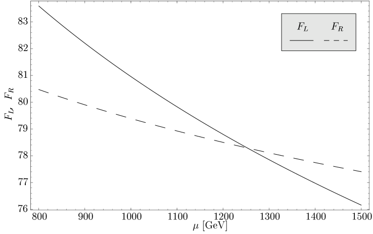
Figure 1: $F_{L}$ and $F_{R}$ in (4.6) as functions of the renormalization scale $\mu$ for central input variables. The unification scale for $M=\tilde{M}$ is uniquely determined by the crossing point.

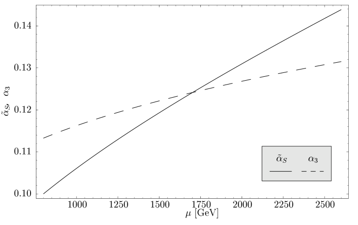
Figure 2: $\alpha_{3}$ and $\tilde{\alpha}_{S}$ as functions of $\mu>\tilde{M}$ for central input variables. The unification scale for $M>\tilde{M}$ is uniquely determined by the crossing point.

In the scenario with $M>\tilde{M}$, the evolution of $\alpha_{1}$, $\alpha_{2}$ and $\alpha_{3}$ for scales $\mu<\tilde{M}$ is as in the scenario with $M=\tilde{M}$, but now the condition (4.5) is replaced by

$$\frac{1}{[\alpha_{1}(\tilde{M}^{2})]}=\frac{C^{2}_{W}}{[\alpha_{2}(\tilde{M}^{2})]}+\frac{C_{S}^{2}}{[\tilde{\alpha}_{S}(\tilde{M}^{2})]}\,,$$ (4.7)

in accordance with (2.28), with $\tilde{\alpha}_{S}$ corresponding to the $U(1)_{S}$ group. Formula (4.7) allows to determine the value of $\tilde{\alpha}_{S}(\tilde{M}^{2})$ at a given scale $\tilde{M}$ that should be larger than $800\,{\rm GeV}$ in order to be consistent with the lower bound on the right–handed gauge boson masses.

Above $\tilde{M}$ the gauge symmetry group is $SU(3)_{c}\otimes U(1)_{S}\otimes SU(2)^{3}$ and the evolution of the gauge couplings must also include the contributions of the Higgs scalars (3.2). The unification scale $M$ is then simply found from the condition

$$\alpha_{3}(M^{2})=\tilde{\alpha}_{S}(M^{2}).$$ (4.8)

This is illustrated graphically in Figure 2. As at the two–loop level the evolutions of the couplings $\alpha_{3}$ and $\tilde{\alpha}_{S}$ are affected by the three $SU(2)$ gauge couplings we also need their values at $\tilde{M}$. This is simply found from

$$\alpha_{2R}(\tilde{M}^{2})=\alpha_{2H}(\tilde{M}^{2})=\alpha_{2L}(\tilde{M}^{2})$$ (4.9)

with $\alpha_{2L}(\tilde{M}^{2})\equiv\alpha_{2}(\tilde{M}^{2})$ calculated as in the scenario with $M=\tilde{M}$.

In what follows we will first give the RG equations relevant for the case $M=\tilde{M}$. Subsequently we will study the scenario with $M>\tilde{M}$.

4.2 Renormalization Group Equations $(M=\tilde{M})$

4.2.1 The Range $M_{Z}\leq\mu\leq M_{F}$

The relevant RG equations for the evolution of the couplings $\alpha_{1}$, $\alpha_{2}$ and $\alpha_{3}$ are given as follows

$$\mu\frac{d\alpha_{i}}{d\mu}=-\frac{\alpha_{i}^{2}}{2\pi}\left[(\beta_{0})_{i}+\sum_{j=1,2,3}(\hat{\beta}_{1})_{ij}\frac{\alpha_{j}}{4\pi}+(\beta_{1})^{Y}_{it}\frac{\lambda_{t}}{4\pi}\right]$$ (4.10)

with $i=1,2,3$ and $\lambda_{t}=g^{2}_{t}/4\pi$, with $g_{t}$ being the Yukawa coupling of the top quark. We neglect the contributions from Yukawa couplings of lighter quarks and from the standard leptons. Moreover as the evolution of the Yukawa couplings is rather involved at the two-loop level, we will keep them at constant values corresponding to $m_{t}(m_{t})$ in the case of the top quark with the same procedure for new heavy quarks and leptons discussed below. This turns out to be a very good approximation in our case, where the evolution of couplings takes place over a rather short range of scales, but of course such a procedure could not be justified in the case of GUTs.

The coefficients $(\beta_{0})_{i}$, $(\hat{\beta}_{1})_{ij}$ and $(\beta_{1})^{Y}_{it}$ are well known but one has to remember that the $U(1)_{Y}$ coupling $\alpha_{1}$ used here is differently normalized than the $\alpha_{1}$ coupling in the $SU(5)$ model. With three generations of quarks and leptons we have then

$$(\beta_{0})_{1}=-\frac{20}{3},\qquad(\beta_{0})_{2}=\frac{10}{3},\qquad(\beta_{0})_{3}=7,$$ (4.11)

$$\hat{\beta}_{1}=\left(\begin{array}[]{ccc}-95/9&-3&-44/3\\ -1&-11/3&-12\\ -11/6&-9/2&26\end{array}\right)$$ (4.12)

and

$$(\beta_{1})^{Y}_{1t}=\frac{17}{6},\qquad(\beta_{1})^{Y}_{2t}=\frac{3}{2},\qquad(\beta_{1})_{3t}^{Y}=2~{}.$$ (4.13)

4.2.2 The Range $M_{F}\leq\mu\leq\tilde{M}$

Above the scale $M_{F}$ the contributions of new fermions in (2.28) and the scalars in (3.4), (3.5) and (3.6) have to be taken into account. This modifies the coefficients in (4.11) and (4.12) as follows

$$(\beta_{0})_{1}=-\frac{136}{3}-\frac{209}{9},\qquad(\beta_{0})_{2}=-\frac{2}{3}-\frac{19}{3},\qquad(\beta_{0})_{3}=3-\frac{16}{3},$$ (4.14)

$$\hat{\beta}_{1}=\left(\begin{array}[]{ccc}-2230/9-17777/27&-42-209&-280/3-3200/9\\ -14-209/3&-158/3-247/3&-24-128\\ -35/3-400/9&-9-48&-50-592/3\end{array}\right),$$ (4.15)

where second terms in (4.14) and (4.15) represent scalar contributions. In addition Yukawa couplings of new quarks and leptons have to be taken into account. With respect to the democratic fermion mass model presented in Section 3.3 the Yukawa term in the RG equations (4.10) is generalized to

$$\Delta_{Y}\left(\mu\frac{d\alpha_{i}}{d\mu}\right)=-\frac{\alpha_{i}^{2}}{2\pi}\sum_{k}(\beta_{1})^{Y}_{ik}\frac{\lambda_{k}}{4\pi},$$ (4.16)

where the sum runs over 13 Yukawa couplings corresponding to seven heavy quarks and six heavy leptons. The coefficients $(\beta_{1})^{Y}_{it}$ are as in (4.13). The coefficients $(\beta_{1})^{Y}_{ik}$ with $k\neq t$ relevant for the contributions of new fermions are found to be

• with respect to $SU(3)_{c}$:

  $$(\beta_{1})^{Y}_{3\tilde{Q}}=2,\qquad\tilde{Q}=\tilde{U},\tilde{D},\tilde{S},\tilde{C},\tilde{B},\tilde{T}$$ (4.17)

• with respect to $SU(2)_{L}$:

  $$(\beta_{1})^{Y}_{2\tilde{Q}} = \frac{3}{2},\qquad\tilde{Q}=\tilde{U},\tilde{D},\tilde{S},\tilde{C},\tilde{B},\tilde{T}$$

  $$(\beta_{1})^{Y}_{2\tilde{L}} = \frac{1}{2},\qquad\tilde{L}=\tilde{l}_{u},\tilde{l}_{d},\tilde{l}_{s},\tilde{l}_{c},\tilde{l}_{b},\tilde{l}_{t}$$ (4.18)

• with respect to $U(1)_{Y}$:

  $$(\beta_{1})^{Y}_{1\tilde{Q}} = \frac{89}{6},\qquad\tilde{Q}=\tilde{U},\tilde{C},\tilde{T}$$

  $$(\beta_{1})^{Y}_{1\tilde{Q}} = \frac{29}{6},\qquad\tilde{Q}=\tilde{D},\tilde{S},\tilde{B}$$

  $$(\beta_{1})^{Y}_{1\tilde{L}} = \frac{13}{2},\qquad\tilde{L}=\tilde{l}_{u},\tilde{l}_{c},\tilde{l}_{t}$$

  $$(\beta_{1})^{Y}_{1\tilde{L}} = \frac{25}{2},\qquad\tilde{L}=\tilde{l}_{d},\tilde{l}_{s},\tilde{l}_{b}~{}.$$ (4.19)

It is clear from these formulae that the Yukawa couplings of $(\tilde{U},\tilde{C},\tilde{T})$, $(\tilde{D},\tilde{S},\tilde{B})$, $(\tilde{l}_{u},\tilde{l}_{c},\tilde{l}_{t})$ and $(\tilde{l}_{d},\tilde{l}_{s},\tilde{l}_{b})$, generally differ from each other. However, in order to get a rough estimate of Yukawa contributions let us set all Yukawa couplings of the new fermions to be equal to the top Yukawa coupling $g_{t}$. Then effectively only the $\lambda_{t}$ term is present as in (4.10) but the coefficients $(\beta_{1})^{Y}_{it}$ are modified as follows

$$(\beta_{1})^{Y}_{1t}=\frac{713}{6},\qquad(\beta_{1})^{Y}_{2t}=\frac{27}{2},\qquad(\beta_{1})_{3t}^{Y}=14.$$ (4.20)

4.2.3 Analytical Formula for $M$

We will present the numerical analysis of this scenario in subsection 4.4. On the other hand it is possible to derive an approximate analytical formula for $M$ as function of the input parameters (4.1), (4.3) and (4.4). To this end we define effective “one loop” coefficients

$$\beta_{i}^{\rm eff}\equiv(\beta_{0})_{i}+\sum_{j=1,2,3}(\hat{\beta}_{1})_{ij}\frac{\alpha_{j}}{4\pi}+(\beta_{1})^{Y}_{it}\frac{\lambda_{t}}{4\pi},$$ (4.21)

with $\alpha_{j}$ and $\lambda_{t}$ frozen at some intermediate scale $M_{Z}\leq\mu\leq M_{F}$. Analogous procedure is used for the range $M_{F}\leq\mu\leq\tilde{M}=M$.

We then find

$$M=M_{F}\left[\frac{M_{Z}}{M_{F}}\right]^{K_{3}/K_{\rm tot}}\exp(P),$$ (4.22)

where

$$P=\frac{1}{8\pi\alpha(M^{2}_{Z})K_{\rm tot}}\left(1-C^{2}_{S}\frac{\alpha(M^{2}_{Z})}{\alpha_{3}(M^{2}_{Z})}-\frac{\sin^{2}\theta_{W}(M_{Z}^{2})}{\sin^{2}\theta_{W}^{0}}\right)$$ (4.23)

and

$$K_{3}=\frac{1}{16\pi^{2}}\left(\beta_{3}^{\rm eff}C_{S}^{2}+\beta_{2}^{\rm eff}C_{W}^{2}-\beta_{1}^{\rm eff}\right)$$ (4.24)

with the RG coefficients given in (4.11)–(4.12). Formula (4.24) is also valid for $K_{\rm tot}$ but this time the coefficients (4.14)-(4.20) relevant for the range $M_{F}\leq\mu\leq\tilde{M}$ should be used. The formula (4.22) can be directly obtained from (2.8) by setting $M=\tilde{M}$ and making the replacement:

$$K\ln\frac{\tilde{M}}{M_{Z}}\to K_{3}\ln\frac{M_{F}}{M_{Z}}+K_{\rm tot}\ln\frac{{M}}{M_{F}}.$$ (4.25)

4.3 Renormalization Group Equations ($M>\tilde{M})$

4.3.1 Preliminaries

The evolution of couplings from $\mu=M_{Z}$ to $\mu=\tilde{M}$ proceeds as in the previous scenario and consequently the formulae given in the subsections 4.1 and 4.2 allow the determination of the couplings $\alpha_{3}(\tilde{M}^{2})$, $\tilde{\alpha}_{S}(\tilde{M}^{2})$, $\alpha_{2L}(\tilde{M}^{2})$, $\alpha_{2R}(\tilde{M}^{2})$ and $\alpha_{2H}(\tilde{M}^{2})$, that constitute the starting point for the subsequent evolution from $\tilde{M}$ to $M$. We already mentioned that the Higgs fields break the equality of the three $SU(2)$ couplings and consequently five different couplings have to be considered, although the splitting of the three $SU(2)$ couplings is insignificant as one can see in Figure 3.

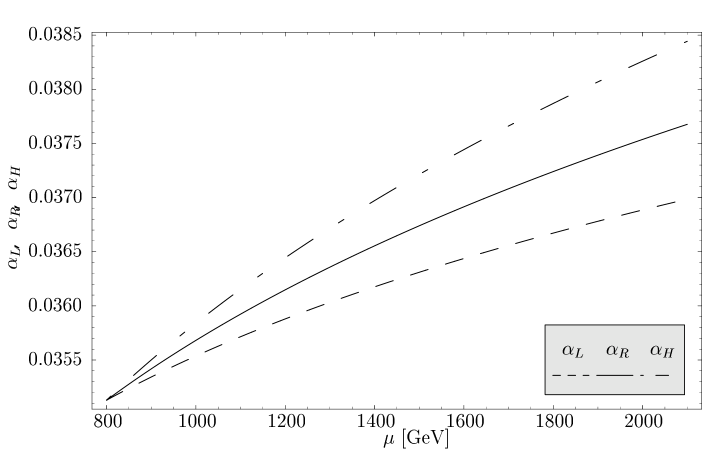
Figure 3: Running of $\alpha_{L}$, $\alpha_{R}$, $\alpha_{H}$ for $M>\tilde{M}$, with all input variables taken at their central values.

4.3.2 The Range $\tilde{M}\leq\mu\leq M$

The relevant RG equations for the evolution of the couplings $\alpha_{3}(\mu^{2})$, $\tilde{\alpha}_{S}(\mu^{2})$, $\alpha_{2L}(\mu^{2})$, $\alpha_{2R}(\mu^{2})$ and $\alpha_{2H}(\mu^{2})$ are given as follows $(i=3,S,2L,2R,2H)$

$$\mu\frac{d\alpha_{i}}{d\mu}=\left(\mu\frac{d\alpha_{i}}{d\mu}\right)_{G}+\Delta_{Y}\left(\mu\frac{d\alpha_{i}}{d\mu}\right),$$ (4.26)

where the first term on the r.h.s describes the evolution of the gauge couplings with all Yukawa couplings set to zero and the second term takes into account the presence of these couplings. We then have

$$\left(\mu\frac{d\alpha_{i}}{d\mu}\right)_{G}=-\frac{\alpha_{i}^{2}}{2\pi}\left[(\beta_{0})_{i}+\sum_{j}(\hat{\beta}_{1})_{ij}\frac{\alpha_{j}}{4\pi}\right],$$ (4.27)

with $j$ running over the five couplings and

$$\Delta_{Y}\left(\mu\frac{d\alpha_{i}}{d\mu}\right)=-\frac{\alpha_{i}^{2}}{2\pi}\sum_{r}(\beta_{1})^{Y}_{ir}\frac{\lambda_{r}}{4\pi},$$ (4.28)

as in (4.16) but this time i=3, S, 2L, 2R, 2H.

With three generations of ordinary and heavy quarks and leptons the coefficients in (4.27) are given as follows (second terms below stand for scalar contributions):

$$(\beta_{0})_{3}=3-\frac{19}{3},\qquad(\beta_{0})_{S}=-8-\frac{19}{3},\qquad(\beta_{0})_{2L}=-\frac{2}{3}-\frac{19}{3},$$

$$(\beta_{0})_{2R}=-\frac{2}{3}-\frac{27}{3},\qquad(\beta_{0})_{2H}=-\frac{26}{3}-\frac{16}{3}$$ (4.29)

and with the ordering $i=3,S,2L,2R,2H$

$$\hat{\beta}_{1}=\left(\hat{\beta}_{1}\right)_{GF}+\left(\hat{\beta}_{1}\right)_{H},$$ (4.30)

where

$$\left(\hat{\beta}_{1}\right)_{GF}=\left(\begin{array}[]{ccccc}-50&-1&-9&-9&-18\\ -8&-7&-9&-9&-18\\ -24&-3&-158/3&0&-18\\ -24&-3&0&-158/3&-18\\ -48&-6&-18&-18&-452/3\end{array}\right)$$ (4.31)

are the contributions arising from fermions and gauge bosons and

$$\left(\hat{\beta}_{1}\right)_{H}=\left(\begin{array}[]{ccccc}-658/3&-67/6&-48&-60&-12\\ -268/3&-277/6&-48&-60&-12\\ -128&-16&-247/3&-57&-24\\ -160&-20&-57&-157&-24\\ -32&-4&-24&-24&-448/3\end{array}\right)$$ (4.32)

are contributions coming from the scalars. With the separation of the scalar contributions the breaking of the symmetry between the $SU(2)$ couplings becomes obvious: $\alpha_{2H}$,$\alpha_{2L}$ and $\alpha_{2R}$ evolve slightly differently. For the coefficients $(\beta_{1})^{Y}_{ir}$ we find

• with respect to $SU(3)_{c}$:

  $$(\beta_{1})^{Y}_{3Q}=2,\qquad Q=~{}{\rm all~{}quarks}$$ (4.33)

• with respect to $SU(2)_{L}$:

  $$(\beta_{1})^{Y}_{2L\tilde{Q}} = \frac{3}{2},\qquad\tilde{Q}=t,\tilde{U},\tilde{D},\tilde{S},\tilde{C},\tilde{B},\tilde{T}$$

  $$(\beta_{1})^{Y}_{2L\tilde{L}} = \frac{1}{2},\qquad\tilde{L}=\tilde{l}_{u},\tilde{l}_{d},\tilde{l}_{s},\tilde{l}_{c},\tilde{l}_{b},\tilde{l}_{t}$$ (4.34)

• with respect to $SU(2)_{R}$:

  $$(\beta_{1})^{Y}_{2R\tilde{Q}} = (\beta_{1})^{Y}_{2L\tilde{Q}},\qquad(\beta_{1})^{Y}_{2R\tilde{L}}=(\beta_{1})^{Y}_{2L\tilde{L}},$$ (4.35)

• with respect to $SU(2)_{H}$:

  $$(\beta_{1})^{Y}_{2H\tilde{Q}} = 3,\qquad\tilde{Q}=t,\tilde{U},\tilde{D},\tilde{S},\tilde{C},\tilde{B},\tilde{T}$$

  $$(\beta_{1})^{Y}_{2H\tilde{L}} = {1},\qquad\tilde{L}=\tilde{l}_{u},\tilde{l}_{d},\tilde{l}_{s},\tilde{l}_{c},\tilde{l}_{b},\tilde{l}_{t}$$ (4.36)

• with respect to $U(1)_{S}$:

  $$(\beta_{1})^{Y}_{SQ}=\frac{1}{2},\qquad{\rm Q=~{}all~{}quarks}$$

  $$(\beta_{1})^{Y}_{SL}=\frac{3}{2},\qquad{\rm L=~{}all~{}leptons}$$ (4.37)

with all remaining coefficients being zero.

Again as in the case of the range $M_{F}\leq\mu\leq\tilde{M}$ we can get a rough estimate of the effects of the Yukawa couplings by setting them equal to each other. In this case

$$\Delta_{Y}\left(\mu\frac{d\alpha_{i}}{d\mu}\right)=-\frac{\alpha_{i}^{2}}{2\pi}(\beta_{1})^{Y}_{i}\frac{\lambda_{Y}}{4\pi},$$ (4.38)

where $\lambda_{Y}$ is universal and

$$(\beta_{1})^{Y}_{3}=14,\qquad(\beta_{1})^{Y}_{1S}=\frac{25}{2},$$ (4.39)

$$(\beta_{1})^{Y}_{2L}=(\beta_{1})^{Y}_{2R}=\frac{27}{2},\qquad(\beta_{1})^{Y}_{2H}=27.$$ (4.40)

4.3.3 Analytic Formula for $M$

Proceeding as in subsection 4.2 one can derive an approximate analytic formula for $M$ as a function of $\tilde{M}$, $M_{F}$ and the input parameters (4.1), (4.3) and (4.4). We find

$$M=\tilde{M}\left[\frac{M_{Z}}{M_{F}}\right]^{K_{3}/K^{\prime}}\left[\frac{M_{F}}{\tilde{M}}\right]^{K_{\rm tot}/K^{\prime}}\exp(P^{\prime}),$$ (4.41)

where

$$P^{\prime}=P\frac{K_{\rm tot}}{K^{\prime}}$$ (4.42)

with $K_{3}$, $K_{\rm tot}$ and $P$ defined in subsection 4.2 and

$$K^{\prime}=\frac{C^{2}_{S}}{16\pi^{2}}\left(\beta_{3}^{\rm eff}-\beta_{S}^{\rm eff}\right)$$ (4.43)

where $\beta_{3}^{\rm eff}$ and $\beta_{S}^{\rm eff}$ are evaluated as in (4.21) but with various coefficients relevant for the range $\tilde{M}\leq\mu\leq M$.

4.4 Numerical Analysis

We have solved the RG equations listed above numerically to find $M=\tilde{M}$ in the first scenario and $M$ in the scenario with $M>\tilde{M}$ and $\tilde{M}\geq 800\,{\rm GeV}$. Let us first neglect the Yukawa contributions. The dependence of $M$ on the input parameters is in the first case as follows:

• As $\sin^{2}\theta_{W}(M_{Z}^{2})$ is very precisely known, the variation of its value within the full range in (4.4) introduces only a shift in the ballpark of $30\,{\rm GeV}$. $M$ decreases with increasing $\sin^{2}\theta_{W}(M_{Z}^{2})$.

• The uncertainty of $M$ due to $M_{F}$ and $\alpha_{3}(M^{2}_{Z})$ is significant as shown in table 1, where we have set $\alpha(M^{2}_{Z})$ and $\sin^{2}\theta_{W}(M_{Z}^{2})$ at their central values and varied $M_{F}$ and $\alpha_{3}(M^{2}_{Z})$ in the ranges given in (4.1) and (4.3). $M$ increases with increasing $M_{F}$ and $\alpha_{3}(M^{2}_{Z})$.

• The effect of the NLO contributions is significant. They increase the scale $M=\tilde{M}$ by roughly 160$\,{\rm GeV}$

In the case $M>\tilde{M}$ our findings are as follows:

• As expected, the value of $M$ increases with decreasing $\tilde{M}$. In table 1 the last two columns show the LO and NLO values of $M$ for $\tilde{M}=800\,{\rm GeV}$. The pattern of the dependence on $M_{F}$ and $\alpha_{3}(M^{2}_{Z})$ is similar to the one in the case $M=\tilde{M}$.

• The NLO corrections in this case are even more important and amount to the increase of $M$ by $370\pm 40\,{\rm GeV}$ for $\tilde{M}=800\,{\rm GeV}$ with a smaller shift for $\tilde{M}>800\,{\rm GeV}$.

Most importantly

• The inspection of the renormalization group coefficients of Sections 4.2 and 4.3 shows that the large impact of NLO corrections originates to a large extent in the scalar contributions.

• Moreover, as discussed below, the latter contributions increase $M$ roughly by $250\,{\rm GeV}$ and $450\,{\rm GeV}$ for $M=\tilde{M}$ and $M>\tilde{M}=800\,{\rm GeV}$, respectively.

Table 1: Values for the unification scale $M$ for various values of $\alpha_{3}(M^{2}_{Z})$ and $M_{F}$, $1/\alpha(M^{2}_{Z})=127.934$ and $\sin^{2}\theta_{W}(M_{Z}^{2})=0.23113)$. In the last two columns we set $\tilde{M}=800\,{\rm GeV}$. The RGEs have been set up including gauge, fermionic and scalar contributions.

$\alpha_{3}(M^{2}_{Z})$	$M_{F}$	$M=\tilde{M},~{}LO$	$M=\tilde{M},~{}NLO$	$M>\tilde{M},~{}LO$	$M>\tilde{M},~{}NLO$
	200	961.4	1120.9	1083.0	1410.4
0.1152	250	1036.7	1180.8	1226.2	1538.6
	300	1102.6	1233.7	1357.2	1655.6
	200	1012.1	1190.4	1178.5	1562.3
0.1172	250	1091.3	1253.0	1334.5	1701.6
	300	1160.7	1308.2	1477.0	1828.9
	200	1063.6	1262.3	1279.0	1726.4
0.1192	250	1146.9	1327.3	1448.2	1877.3
	300	1219.7	1385.0	1602.9	2015.2

In summary, varying all the input parameters within one standard deviation we find at the NLO level

$$M=(1253\pm 132)\,{\rm GeV},\qquad(M=\tilde{M})$$ (4.44)

and

$$M=(1713\pm 302)\,{\rm GeV},\qquad(M>\tilde{M}=800\,{\rm GeV}).$$ (4.45)

4.5 Anatomy of Renormalization Group Effects

In what follows we would like to present the results of a number of exercises that we made in the context of our numerical analysis.

First the inclusion of Yukawa couplings changes the values in (4.44) and (4.45) respectively to

$$M=(1273\pm 132)\,{\rm GeV},\qquad(M=\tilde{M})$$ (4.46)

and

$$M=(1742\pm 300)\,{\rm GeV},\qquad(M>\tilde{M}=800\,{\rm GeV}).$$ (4.47)

The relatively small impact of Yukawa couplings on our results justifies our rough treatment of these contributions.

Next, removing the scalar contributions altogether we find instead of (4.44) and (4.45)

$$M=(994\pm 120)\,{\rm GeV},\qquad(M=\tilde{M})$$ (4.48)

and

$$M=(1254\pm 300)\,{\rm GeV},\qquad(M>\tilde{M}=800\,{\rm GeV}),$$ (4.49)

implying that these contributions are very important.

Finally, we have investigated the impact of the increase of $M_{F}$ to $M=\tilde{M}$. This is equivalent to the removal of the heavy fermion contributions to the renormalization group equations below the unification scale. We find then for the maximal unification scale obtained with largest $\alpha_{3}(M_{Z}^{2})$ and smallest $\sin^{2}\theta_{W}(M_{Z}^{2})$

$$M_{\rm max}=\tilde{M}=M_{F}=4595~{}(2442)\,{\rm GeV}$$ (4.50)

with and (without) scalar contributions (at the scale 250  GeV), respectively. Thus even without heavy fermions below $\mu=M$ we obtain a relatively low unification scale. That is, the group theoretic factors $C_{S}$ and $C_{W}$ in our master formula guarantee early unification even if only the SM fields have masses below the unification scale. On the other hand the presence of new heavy fermions with masses $\mathcal{O}\left(250\,\rm{GeV}\right)$ is necessary in order to keep $M$ below $2~{}\rm{TeV}$.

5 The Fate of the Unconventional Fermions

5.1 Relevant Interactions

As we have shown in [6] and in Section 2.4, the construction of the model necessitates the introduction of new heavy quarks and leptons with unconventional charges: $\pm 4/3$ for the quarks and $\pm 2$ for the leptons. These fermions behave in exactly the same manner as the ordinary fermions and are linked to the latter by $SU(2)_{H}$ gauge interactions $g_{W}\bar{\Psi}_{L,R}\vec{W}_{\mu H}.\vec{T}_{H}\,\gamma^{\mu}\Psi_{L,R}$, and by the Yukawa interactions $g_{\Phi_{H}}\bar{\Psi}_{L}\vec{\Phi}_{H}.\vec{T}_{H}\Psi_{R}$. The question arises as to the fate of the lightest of these new fermions.

One should note that the vector-like quarks and leptons as written down in [6] and (2.29) suffer from problems with cosmological constraints in the following way. Since they carry electric charges such as 5/6 or 3/2, the lightest one would be absolutely stable since it cannot decay into known particles. There are severe constraints on objects such as stable fractionally charged leptons [17] and, unless the numbers are severely depleted by exotic mechanisms such as the one proposed in [17], they are ruled out observationally. We will therefore omit them altogether.

Let us first discuss the fate of the unconventional $SU(2)_{H}$ partners of standard quarks and leptons by looking only at the gauge interactions. For the lightest new quark, if the gauge bosons do not mix, one would face the dreadful conclusion that it would be absolutely stable. We will discuss below various constraints which rule out that situation. Fortunately, we will see that there are Higgs fields whose VEVs mix the gauge bosons of the different groups and it is this mixing which renders the lightest new quark unstable, i.e. it can now decay into conventional fermions which are assumed to be lighter. A similar argument applies to the case of the new leptons.

In this section, we focus only on the charge-changing interactions and hence on the charged gauge bosons of $SU(2)_{L}\otimes SU(2)_{R}\otimes SU(2)_{H}$. We have already discussed above the breaking of $SU(2)_{R}\otimes SU(2)_{H}$ and, in particular, the neutral gauge boson sector. In that discussion, we have used the Higgs fields $\Delta_{R}=(4,1,3,1)$ and $\Delta_{H}=(4,1,1,3)$. However, as we have shown in Sections 3.1 and 3.2, other Higgs fields come into play, namely $\Phi=(1,2,2,1)$, $\Phi_{H}=(1,2,2,3)$ as well as $\phi^{(1)}$ which is the color singlet part of $\phi^{\beta}=(15,2,2,1)$. The VEVs of these scalars will evidently mix various gauge bosons. We have also mentioned earlier that, for symmetry reasons, one would also like to have $\Delta_{L}=(4,3,1,1)$, $\tilde{\Phi}_{1}=(1,2,1,2)$ and $\tilde{\Phi}_{2}=(1,1,2,2)$. A detailed treatment of this problem is given in Appendix A. Here we will give a simplified version for illustration. In particular, we will make the same assumption as in (3.68), namely $\delta_{R}=\delta_{H}=\delta$. Furthermore, we will assume that $\delta>\langle\tilde{\Phi}_{2}\rangle\gg\langle\Phi\rangle,\,\langle\Phi_{H}\rangle,\,\langle\tilde{\Phi}_{1}\rangle,\,\langle\phi^{(1)}\rangle$. For simplicity, we will also assume that $\langle\Delta_{L}\rangle=0$. Below, we will denote a generic electroweak scale by $v$ and a generic large scale by $\delta$.

Since this section focuses primarily on the question of whether or not the lightest of the unconventional fermions are stable, we will present a streamlined version of the discussion which will accurately summarize the points that we wish to make. Some of the details can be found in Appendix A.

The lightest of the unconventional fermions can only decay into either a conventional fermion plus the SM $W$ boson or into three conventional fermions if it has the appropriate mass. This implies that the current $J^{\mu}_{H}$ should interact with the SM $W$ for the former case or it mixes with either $J^{\mu}_{L}$ or $J^{\mu}_{R}$ for the latter case. This is what we will show below. We use the notation $g_{W}$ for the three gauge couplings which are defined to be equal to each other at $\tilde{M}$ (see (2.11). In the estimate of the decay rates given below, we shall, however, take the value of $g_{2}$ or equivalently of the Fermi constant $G_{F}$ for simplicity.

With the above remarks taken into account, we now list the eigenvalues and mass eigenstates for the charged gauge bosons. (The exact expressions with various factors included are given in Appendix A.) Our notations are as follows. We use $\tilde{W}_{L},W_{1},W_{2}$ for the mass eigenstates and $W_{L},W_{R},W_{H}$ for the gauge eigenstates. We have

$$M_{\tilde{W}_{L}}=\mathcal{O}(g_{W}\,v),\quad M_{W_{1}}=\mathcal{O}(g_{W}\,\delta),\quad M_{W_{2}}=\mathcal{O}(g_{W}\,\delta).$$ (5.1)

The relationship between the gauge and mass eigenstates is given by

$$\left(\begin{array}[]{c}W_{L}^{\pm}\\ W_{R}^{\pm}\\ W_{H}^{\pm}\end{array}\right)=O^{T}\left(\begin{array}[]{c}\tilde{W}_{L}^{\pm}\\ W_{1}^{\pm}\\ W_{2}^{\pm}\end{array}\right)=\left(\begin{array}[]{ccc}1&{\cal{O}}(v^{2}/\delta^{2})&{\cal{O}}(v^{2}/\delta^{2})\\ {\cal{O}}(v^{2}/\delta^{2})&\frac{1}{\sqrt{2}}&\frac{1}{\sqrt{2}}\\ {\cal{O}}(v^{2}/\delta^{2})&\frac{1}{\sqrt{2}}&-\frac{1}{\sqrt{2}}\end{array}\right)\left(\begin{array}[]{c}\tilde{W}_{L}^{\pm}\\ W_{1}^{\pm}\\ W_{2}^{\pm}\end{array}\right).$$ (5.2)

Let us denote generically the charge-changing currents associated with $SU(2)_{L}$, $SU(2)_{R}$, and $SU(2)_{H}$ by $J^{\mu}_{L}$, $J^{\mu}_{R}$, and $J^{\mu}_{H}$ respectively. The charged current interactions involving these currents can now be written as (with $\pm$ omitted for simplicity)

$${\cal L}_{interaction}=g_{W}(J^{\mu}_{L},J^{\mu}_{R},J^{\mu}_{H})\times\left(\begin{array}[]{c}W_{\mu\,L}\\ W_{\mu\,R}\\ W_{\mu\,H}\end{array}\right)\,.$$ (5.3)

In terms of the gauge boson mass eigenstates, one can now write (5.3) as

$${\cal L}_{interaction}=g_{W}(\tilde{J}^{\mu}_{L},\tilde{J}^{\mu}_{R},\tilde{J}^{\mu}_{H})\times\left(\begin{array}[]{c}\tilde{W}_{\mu\,L}\\ W_{\mu\,1}\\ W_{\mu\,2}\end{array}\right)\,,$$ (5.4)

where

$$(\tilde{J}^{\mu}_{L},\tilde{J}^{\mu}_{R},\tilde{J}^{\mu}_{H})=(J^{\mu}_{L},J^{\mu}_{R},J^{\mu}_{H})\times O^{T}\,,$$ (5.5)

and where the rotation matrix $O^{T}$ is given in (5.2). Explicitely, we now list separately the following interactions.

• Interaction with $\tilde{W}_{\mu\,L}$:

  $${\cal L}_{L} = g_{W}\,\tilde{J}^{\mu}_{L}\tilde{W}_{\mu\,L}$$ (5.6)

  $$= g_{W}[J^{\mu}_{L}+{\cal{O}}(v^{2}/\delta^{2})(J^{\mu}_{R}+J^{\mu}_{H})]\tilde{W}_{\mu\,L}$$

• Interaction with $W_{\mu\,1}$:

  $${\cal L}_{1} = g_{W}\,\tilde{J}^{\mu}_{R}W_{\mu\,1}$$ (5.7)

  $$= g_{W}[{\cal{O}}(v^{2}/\delta^{2})J^{\mu}_{L}+\frac{1}{\sqrt{2}}(J^{\mu}_{R}+J^{\mu}_{H})]W_{\mu\,1}$$

• Interaction with $W_{\mu\,2}$:

  $${\cal L}_{2} = g_{W}\,\tilde{J}^{\mu}_{H}W_{\mu\,2}$$ (5.8)

  $$= g_{W}[{\cal{O}}(v^{2}/\delta^{2})J^{\mu}_{L}+\frac{1}{\sqrt{2}}(J^{\mu}_{R}-J^{\mu}_{H})]W_{\mu\,2}$$

A few remarks are in order here.

• From (5.6), we observe that the contribution of a $V+A$ current to known weak interactions is suppressed in the interaction Lagrangian by a factor ${\cal{O}}(v^{2}/\delta^{2})$. Experimental constraints [15] from searches for right-handed currents in normal weak interactions give ${\cal{O}}(v^{2}/\delta^{2})<10^{-3}$. This can easily be satisfied within our model through the choices of the various VEVs.

• Also from (5.6), one can see that $J^{\mu}_{H}$, which changes a conventional fermion into an unconventional one and vice versa, couples with $\tilde{W}_{\mu\,L}$ with a factor ${\cal{O}}(v^{2}/\delta^{2})$. This has some important implications concerning the decay of the lightest of the unconventional fermions.

  1) If the lightest unconventional fermion which appears in $J^{\mu}_{H}$ has a mass greater than the sum of the accompanying conventional fermion mass and the W-boson mass, it can have the decay mode $\tilde{F}\rightarrow f+W$ ($W$ being the standard $\tilde{W}_{\mu\,L}$) via the interaction

  $$g_{W}{\cal{O}}(v^{2}/\delta^{2})J^{\mu}_{H}\tilde{W}_{\mu\,L}.$$ (5.9)

  Even though ${\cal{O}}(v^{2}/\delta^{2})<10^{-3}$, the decay rate can be substantial because the unconventional fermion decays into a real $W_{L}$.

  2) If the mass of the lightest unconventional fermion is less than the sum of the $W$-mass and the mass of the accompanying conventional fermion, the decay can occur through the interaction:

  $$2g_{W}^{2}{\cal{O}}(v^{2}/\delta^{2})J^{\mu}_{L}\,\frac{1}{q^{2}-m_{\tilde{W}_{L}}^{2}}\,J_{\mu H}.$$ (5.10)

• If the mass of the unconventional fermion is between the sum of the accompanying conventional fermion mass and the $W$-boson mass and either that of $W_{1}$ or $W_{2}$, the decay would be into a real $W_{L}$ as in (1) above.

• If the mass of the lightest unconventional fermion is less than the sum of the $W$-mass and the mass of the accompanying conventional fermion then, from (5.7) and (5.8), one obtains the following additional contributions to the decay:

  $$g_{W}^{2}J^{\mu}_{R}(\frac{1}{q^{2}-m_{W1}^{2}}-\frac{1}{q^{2}-m_{W2}^{2}})J_{\mu H}.$$ (5.11)

In computing the matrix elements for various decays, one has to express the fermions which appear in $J^{\mu}_{L}$, $J^{\mu}_{R}$ and $J^{\mu}_{H}$ in terms of the mass eigenstates. This will result in the appearance of a number of mixing angles which are different from the CKM elements. In the absence of a plausible model of fermion masses (especially for the unconventional ones), the best one can do is to make estimates of the decay rates based on reasonable assumptions about the magnitudes of these unknown mixing angles.

5.2 Decay Modes

We will present here some estimates of possible decay modes of the lightest unconventional quark and lepton. The main purpose, as we have mentioned above, is to see how fast or how slow these fermions decay. Since there are strong constraints on “stable” fermions from cosmology and from collider experiments, the unconventional fermions should be sufficiently heavy and should decay fast enough to evade these bounds. This is what we will show below. A comprehensive study of all possible decays is beyond the scope of this paper and it will be included in a future publication. Here we wish to merely present some illustrative examples.

To be more specific, let us assume that the lightest unconventional quark is $\tilde{U}(4/3)$ and the lightest unconventional lepton is $\tilde{l}_{u}(-1)$, where the numbers inside the parentheses represent the charges of these particles. (One can easily change this scenario to, e.g., $\tilde{D}(1/3)$ and $\tilde{l}_{d}(-2)$, or any other combination.) Since those lightest unconventional fermions cannot decay into other unconventional fermions, the only option left is for them to decay into conventional fermions.

In what follows, we will use the following notations for the conventional fermions: $\psi^{i}_{d}=d,s,b$ and $\psi^{i}_{\nu}=\nu_{e},\nu_{\mu},\nu_{\tau}$, for the quarks and the neutral leptons respectively. Notice that $SU(2)_{H}$ interactions connect $\tilde{U}(4/3)$ to $\bar{\psi}^{i}_{d}$, and $\tilde{l}_{u}(-1)$ to $\psi^{i}_{\nu}$.

In using $J^{\mu}_{H}$, we will express the fields which appear in that current in terms of their mass eigenstates. Consequently, the results presented below will contain mixing angles of the type $V_{\tilde{U}\,\psi^{i}_{d}}$.

• $\tilde{U}(4/3)$ decay:

  We now consider the following possibility: $M(\tilde{U}(4/3))>m(\psi^{i}_{d})+M_{\tilde{W}_{\mu\,L}}$. This case is more or less obvious since we require the unconventional fermions to be heavy, i.e. around $250\,{\rm GeV}$ or so.

  In this case, the dominant decay mode would be the semi-weak process:

  $$\tilde{U}(4/3)\rightarrow\bar{\psi}^{i}_{d}+\tilde{W}^{+}_{\mu\,L}\,.$$ (5.12)

  Since, by assumption, $m^{2}_{d,s,b}/M^{2}_{\tilde{U}}\ll 1$, one can immediately find the following decay width:

  $$\Gamma=(\frac{G_{F}M^{3}_{\tilde{U}}}{8\pi\sqrt{2}})\,|{\cal{O}}(v^{2}/\delta^{2})|^{2}\,|V_{\tilde{U}\,\psi^{i}_{d}}|^{2}\,(1-\frac{M^{2}_{\tilde{W}_{\mu\,L}}}{M^{2}_{\tilde{U}}})^{2}\,(1+\frac{2\,M^{2}_{\tilde{W}_{\mu\,L}}}{M^{2}_{\tilde{U}}}),\,$$ (5.13)

  where $G_{F}$ is the Fermi constant. For $M_{\tilde{U}}\approx 250\,GeV$, one obtains

  $$\Gamma_{\tilde{U}}\approx 6\,|V_{\tilde{U}\,\psi^{i}_{d}}|^{2}\,|{\cal{O}}(v^{2}/\delta^{2})|^{2}\,\,{\rm GeV}\,,$$ (5.14)

  where $V_{\tilde{U}\,\psi^{i}_{d}}$ is the matrix element of $V=U^{-1}_{D}U_{\tilde{U}}$. The matrices $U_{D}$ and $U_{\tilde{U}}$ are those that diagonalize the mass matrices of the conventional Down-quark sector and the unconventional Up-quark sector, respectively.

  The mean lifetime is found to be

  $$\tau_{\tilde{U}}\approx 1.1\times 10^{-25}|V_{\tilde{U}\,\psi^{i}_{d}}|^{-2}\,|{\cal{O}}(v^{2}/\delta^{2})|^{-2}\,s\,.$$ (5.15)

  For illustration, let us put ${\cal{O}}(v^{2}/\delta^{2})\approx 10^{-3}$ as we have mentioned above. The mean lifetime is $\tau_{\tilde{U}}\approx 1.1\times 10^{-19}|V_{\tilde{U}\,\psi^{i}_{d}}|^{-2}\,s$. One can see that $\tilde{U}$ can decay very fast unless the mixing $V_{\tilde{U}\,\psi^{i}_{d}}$ is abnormally small.

  For a particle which decays that fast, there is no cosmological constraint. It can be searched for at future facilities such as the Large Hadron Collider. This type of search was discussed at length in [16].

• $\tilde{l}_{u}(-1)$ decay:

  The computation for the decay rate here is very similar to that presented above. We will assume that the mass of $\tilde{l}_{u}(-1)$ is comparable to that of $\tilde{U}$. The main decay mode is then

  $$\tilde{l}_{u}(-1)\rightarrow\psi^{i}_{\nu}+\tilde{W}^{-}_{\mu\,L}\,,$$ (5.16)

  where $\psi^{i}_{\nu}=\nu_{e},\nu_{\mu},\nu_{\tau}$.

  Once again we will assume that $M_{\tilde{l}_{u}}\approx 250\,GeV$. The decay width is then found to be

  $$\Gamma_{\tilde{l}_{u}}\approx 6\,|V_{\tilde{l}_{u}\,\psi^{i}_{\nu}}|^{2}\,|{\cal{O}}(v^{2}/\delta^{2})|^{2}\,\,{\rm GeV}\,.$$ (5.17)

  Its mean lifetime could be very short, i.e. $\tau_{\tilde{l}_{u}}\approx 1.1\times 10^{-19}|V_{\tilde{l}_{u}\,\psi^{i}_{\nu}}|^{-2}\,s$, if $|V_{\tilde{l}_{u}\,\psi^{i}_{\nu}}|^{2}$ is not abnormally small. Again there is no cosmological constraint. A discussion of the search for leptons of this type can be found in [16].

As we have mentioned above, although we have chosen $\tilde{U}$ and $\tilde{l}_{u}$ to illustrate how an unconventional fermion can decay entirely into conventional particles, one can choose other unconventional fermions to be the lightest ones and study their decays. This will be presented elsewhere. The main point in this section was to show that, because of mixing among the various gauge bosons, the lightest unconventional quark or lepton is fairly unstable, and, for the range of masses that we consider, decays mainly into a real $W$ and a conventional fermion.

6 Summary

In this paper we have extended the discussion of the early unification of quarks and leptons based on the gauge group $SU(4)_{\rm PS}\otimes SU(2)_{L}\otimes SU(2)_{R}\otimes SU(2)_{H}$ [6]. In particular

• we have presented the Higgs system which accomplishes the spontaneous symmetry breaking (SSB) of the gauge group $G_{\rm PUT}$ down to the $SU(3)_{c}\otimes U(1)_{\rm QED}$ group with the acceptable spectrum of gauge boson, fermion and Higgs masses.

• we have shown that the inclusion of NLO effects and of Higgs scalars into the renormalization group analysis increases the unification scale $M$, relatively to the estimates in [6], by roughly $250\,{\rm GeV}$ and $450\,{\rm GeV}$ for $M=\tilde{M}$ and $M>\tilde{M}=800\,{\rm GeV}$, respectively. This allows still for a unification of quarks and leptons at scales ${\cal O}(1-2~{}{\rm TeV})$. Specifically in the two scenario considered we find

  $$M=(1253\pm 132)\,{\rm GeV},\qquad(M=\tilde{M})$$ (6.1)

  and

  $$M=(1713\pm 302)\,{\rm GeV},\qquad(M>\tilde{M}\geq 800\,{\rm GeV}).$$ (6.2)

• we have shown that the presence of three new generations of heavy unconventional quarks and leptons with masses ${\cal O}(250\,{\rm GeV})$ is consistent with constraints coming from cosmology.

A detailed discussion of the rare decay $K_{L}\to\mu e$ and of FCNC processes will be presented elsewhere.

Acknowledgements
The work presented here was supported in part by DFG Project Bu. 706/1-2. P.Q.H. and N.K.T. are supported by the US Department of Energy under Grant No. DE-A505-89ER40518.

Appendix A Appendix A

In this Appendix we present the mixing of gauge bosons following the symmetry breaking of $U(1)_{S}\otimes SU(2)_{L}\otimes SU(2)_{R}\otimes SU(2)_{H}\rightarrow U(1)_{Y}\otimes SU(2)_{L}\rightarrow U(1)_{QED}$.

A.1 Neutral gauge boson mixing

The mixing of neutral gauge bosons $W_{3R}$, $W_{3H}$, $\tilde{A}_{S}$ is given by the VEV of $\Delta_{R}(4,1,3,1)$ and $\Delta_{H}(4,1,1,3)$ (considering only color singlet part)

$$\langle\Delta_{R}\rangle=\left(\begin{array}[]{cc}0&\delta_{R}/\sqrt{2}\\ 0&0\end{array}\right),$$ (A.1)

$$\langle\Delta_{H}\rangle=\left(\begin{array}[]{cc}0&\delta_{H}/\sqrt{2}\\ 0&0\end{array}\right)$$ (A.2)

with the corresponding covariant derivatives

$$D_{\mu}\Delta_{R}=\partial_{\mu}\Delta_{R}-i\sqrt{3/8}\;\tilde{g}_{S}\tilde{A}_{\mu S}(-1)\Delta_{R}-ig_{W}[W^{a}_{\mu R}\frac{\tau^{a}}{2},\Delta_{R}],$$ (A.3)

$$D_{\mu}\Delta_{H}=\partial_{\mu}\Delta_{H}-i\sqrt{3/8}\;\tilde{g}_{S}\tilde{A}_{\mu S}(-1)\Delta_{H}-ig_{W}[W^{a}_{\mu H}\frac{\tau^{a}}{2},\delta_{H}]$$ (A.4)

and

$$W^{a}_{\mu}\frac{\tau^{a}}{2}=\frac{1}{2}\left(\begin{array}[]{cc}W_{\mu 3}&\sqrt{2}W_{\mu}^{+}\\ \sqrt{2}W_{\mu}^{-}&-W_{\mu 3}\end{array}\right).$$ (A.5)

From $Tr\left(D_{\mu}\Delta_{R}^{\dagger}D^{\mu}\Delta_{R}\right)$ and $Tr\left(D_{\mu}\Delta_{H}^{\dagger}D^{\mu}\Delta_{H}\right)$ follows the squared mass matrix of neutral gauge bosons

$$\left(\begin{array}[]{ccc}g_{W}^{2}\delta_{R}^{2}&0&-\sqrt{3/8}\;g_{W}\tilde{g}_{S}\delta_{R}^{2}\\ 0&g_{W}^{2}\delta_{H}^{2}&-\sqrt{3/8}\;g_{W}\tilde{g}_{S}\delta_{H}^{2}\\ -\sqrt{3/8}\;g_{W}\tilde{g}_{S}\delta_{R}^{2}&-\sqrt{3/8}\;g_{W}\tilde{g}_{S}\delta_{H}^{2}&\frac{3}{8}g_{S}^{2}(\delta_{R}^{2}+\delta_{H}^{2})\end{array}\right).$$ (A.6)

This matrix can be diagonalized by an orthogonal matrix $O$:

$$O\left(\begin{array}[]{ccc}g_{W}^{2}\delta_{R}^{2}&0&-\sqrt{3/8}\;g_{W}\tilde{g}_{S}\delta_{R}^{2}\\ 0&g_{W}^{2}\delta_{H}^{2}&-\sqrt{3/8}\;g_{W}\tilde{g}_{S}\delta_{H}^{2}\\ -\sqrt{3/8}\;g_{W}\tilde{g}_{S}\delta_{R}^{2}&-\sqrt{3/8}\;g_{W}\tilde{g}_{S}\delta_{H}^{2}&\frac{3}{8}\tilde{g}_{S}^{2}(\delta_{R}^{2}+\delta_{H}^{2})\end{array}\right)O^{T}=\left(\begin{array}[]{ccc}0&0&0\\ 0&M_{Z_{1}}^{2}&0\\ 0&0&M_{Z_{2}}^{2}\end{array}\right)$$ (A.7)

with

$$\left(\begin{array}[]{c}B\\ Z_{1}\\ Z_{2}\end{array}\right)=O\left(\begin{array}[]{c}W_{3R}\\ W_{3H}\\ \tilde{A}_{s}\end{array}\right).$$ (A.8)

This diagonalization gives the following general result:

1) massless (normalized) eigenvector

$$\left(\frac{\sqrt{3}\tilde{g}_{S}}{\sqrt{6\tilde{g}_{S}^{2}+8g_{W}^{2}}};\frac{\sqrt{3}\tilde{g}_{S}}{\sqrt{6\tilde{g}_{S}^{2}+8g_{W}^{2}}};\frac{2\sqrt{2}g_{W}}{\sqrt{6\tilde{g}_{S}^{2}+8g_{W}^{2}}}\right).$$ (A.9)

2) 1st massive neutral boson

$$M_{Z1}^{2}=\frac{1}{2}\left[(\delta_{R}^{2}+\delta_{H}^{2})(g_{W}^{2}+3\tilde{g}_{S}^{2}/8)-\sqrt{(\delta_{R}^{2}+\delta_{H}^{2})^{2}(g_{W}^{2}+3\tilde{g}_{S}^{2}/8)^{2}-g_{W}^{2}\delta_{R}^{2}\delta_{H}^{2}(4g_{W}^{2}+3\tilde{g}_{S}^{2})}\right]$$ (A.10)

with corresponding (not-yet-normalized) eigenvector

$$\left(-\frac{g_{W}\sqrt{8}\left[(\delta_{H}^{2}-\delta_{R}^{2})(g_{W}^{2}+3\tilde{g}_{S}^{2}/8)+\sqrt{(\delta_{R}^{2}+\delta_{H}^{2})^{2}(g_{W}^{2}+3\tilde{g}_{S}^{2}/8)^{2}-g_{W}^{2}\delta_{R}^{2}\delta_{H}^{2}(4g_{W}^{2}+3\tilde{g}_{S}^{2})}\right]}{\tilde{g}_{S}\sqrt{3}\left[g_{W}^{2}(\delta_{H}^{2}-\delta_{R}^{2})-3\tilde{g}_{S}^{2}(\delta_{R}^{2}+\delta_{H}^{2})/8+\sqrt{(\delta_{R}^{2}+\delta_{H}^{2})^{2}(g_{W}^{2}+3\tilde{g}_{S}^{2}/8)^{2}-g_{W}^{2}\delta_{R}^{2}\delta_{H}^{2}(4g_{W}^{2}+3\tilde{g}_{S}^{2})}\right]};\right.$$

$$\left.\frac{\sqrt{3/2}\;g_{W}\tilde{g}_{S}\delta_{H}^{2}}{g_{W}^{2}(\delta_{H}^{2}-\delta_{R}^{2})-3\tilde{g}_{S}^{2}(\delta_{R}^{2}+\delta_{H}^{2})/8+\sqrt{(\delta_{R}^{2}+\delta_{H}^{2})^{2}(g_{W}^{2}+3\tilde{g}_{S}^{2}/8)^{2}-g_{W}^{2}\delta_{R}^{2}\delta_{H}^{2}(4g_{W}^{2}+3\tilde{g}_{S}^{2})}};1\right).$$

3) 2nd massive neutral boson

$$M_{Z2}^{2}=\frac{1}{2}\left[(\delta_{R}^{2}+\delta_{H}^{2})(g_{W}^{2}+3\tilde{g}_{S}^{2}/8)+\sqrt{(\delta_{R}^{2}+\delta_{H}^{2})^{2}(g_{W}^{2}+3\tilde{g}_{S}^{2}/8)^{2}-g_{W}^{2}\delta_{R}^{2}\delta_{H}^{2}(4g_{W}^{2}+3\tilde{g}_{S}^{2})}\right]$$ (A.11)

with corresponding (not-yet-normalized) eigenvector

$$\left(-\frac{g_{W}\sqrt{8}\left[(\delta_{H}^{2}-\delta_{R}^{2})(g_{W}^{2}+3\tilde{g}_{S}^{2}/8)-\sqrt{(\delta_{R}^{2}+\delta_{H}^{2})^{2}(g_{W}^{2}+3\tilde{g}_{S}^{2}/8)^{2}-g_{W}^{2}\delta_{R}^{2}\delta_{H}^{2}(4g_{W}^{2}+3\tilde{g}_{S}^{2})}\right]}{\tilde{g}_{S}\sqrt{3}\left[g_{W}^{2}(\delta_{H}^{2}-\delta_{R}^{2})-3\tilde{g}_{S}^{2}(\delta_{R}^{2}+\delta_{H}^{2})/8-\sqrt{(\delta_{R}^{2}+\delta_{H}^{2})^{2}(g_{W}^{2}+3\tilde{g}_{S}^{2}/8)^{2}-g_{W}^{2}\delta_{R}^{2}\delta_{H}^{2}(4g_{W}^{2}+3\tilde{g}_{S}^{2})}\right]};\right.$$

$$\left.\frac{\sqrt{3/2}\;g_{W}\tilde{g}_{S}\delta_{H}^{2}}{g_{W}^{2}(\delta_{H}^{2}-\delta_{R}^{2})-3\tilde{g}_{S}^{2}(\delta_{R}^{2}+\delta_{H}^{2})/8-\sqrt{(\delta_{R}^{2}+\delta_{H}^{2})^{2}(g_{W}^{2}+3\tilde{g}_{S}^{2}/8)^{2}-g_{W}^{2}\delta_{R}^{2}\delta_{H}^{2}(4g_{W}^{2}+3\tilde{g}_{S}^{2})}};1\right).$$

A special situation where $\delta_{R}^{2}=\delta_{H}^{2}$ has been also discussed in the main text.

A.2 Charged gauge boson mixing

The mixing of charged gauge bosons $W_{L}^{\pm}$, $W_{R}^{\pm}$, $W_{H}^{\pm}$ is given by the VEV of $\Delta_{R}(4,1,3,1)$, $\Delta_{H}(4,1,1,3)$ (see above), $\Phi(1,2,2,1)$, $\tilde{\Phi}_{1}(1,2,1,2)$, $\tilde{\Phi}_{2}(1,1,2,2)$, $\phi_{s}(15,2,2,1)$, $\Phi_{H}(1,2,2,3)$:

• $$\langle\Phi\rangle=\left(\begin{array}[]{cc}v_{1}/\sqrt{2}&0\\ 0&v_{2}/\sqrt{2}\end{array}\right),$$ (A.12)

• $$\langle\tilde{\Phi}_{1}\rangle=\left(\begin{array}[]{cc}u_{1}/\sqrt{2}&0\\ 0&u_{2}/\sqrt{2}\end{array}\right),$$ (A.13)

• $$\langle\tilde{\Phi}_{2}\rangle=\left(\begin{array}[]{cc}w_{1}/\sqrt{2}&0\\ 0&w_{2}/\sqrt{2}\end{array}\right),$$ (A.14)

• $$\langle\phi_{s}\rangle=\left(\begin{array}[]{cc}v^{\prime}_{1}&0\\ 0&v^{\prime}_{2}\end{array}\right)\otimes\frac{1}{2\sqrt{6}}\left(\begin{array}[]{cccc}1&0&0&0\\ 0&1&0&0\\ 0&0&1&0\\ 0&0&0&-3\end{array}\right),$$ (A.15)

• $$\langle\Phi_{H}\rangle=\left(\begin{array}[]{cccc}\chi_{1}/2&0&0&0\\ 0&\chi_{2}/2&0&0\\ 0&0&-\chi_{1}/2&0\\ 0&0&0&-\chi_{2}/2\end{array}\right),$$ (A.16)

with the corresponding covariant derivative

$$D_{\mu}\Phi=\partial_{\mu}\Phi-ig_{W}[W^{a}_{\mu L}\frac{\tau^{a}}{2}]\Phi-ig_{W}\Phi[W^{a}_{\mu R}\frac{\tau^{a}}{2}],$$ (A.17)

$$D_{\mu}\tilde{\Phi}_{1}=\partial_{\mu}\tilde{\Phi}_{1}-ig_{W}[W^{a}_{\mu L}\frac{\tau^{a}}{2}]\tilde{\Phi}_{1}-ig_{W}\tilde{\Phi}_{1}[W^{a}_{\mu H}\frac{\tau^{a}}{2}],$$ (A.18)

$$D_{\mu}\tilde{\Phi}_{2}=\partial_{\mu}\tilde{\Phi}_{2}-ig_{W}[W^{a}_{\mu R}\frac{\tau^{a}}{2}]\tilde{\Phi}_{2}-ig_{W}\tilde{\Phi}_{2}[W^{a}_{\mu H}\frac{\tau^{a}}{2}],$$ (A.19)

$$D_{\mu}\phi_{s}\supset\partial_{\mu}\phi_{s}-ig_{W}[W^{a}_{\mu L}\frac{\tau^{a}}{2}]\otimes\phi_{s}-ig_{W}\phi_{s}\otimes[W^{a}_{\mu R}\frac{\tau^{a}}{2}],$$ (A.20)

$$D_{\mu}\phi_{223}=\partial_{\mu}\phi_{223}-ig_{W}[W^{a}_{L\mu}\frac{\tau^{a}}{2}]\otimes\phi_{223}-ig_{W}\phi_{223}\otimes[W^{a}_{R\mu}\frac{\tau^{a}}{2}]-ig_{W}[W^{a}_{H\mu}\frac{\tau^{a}}{2},\phi_{223}].$$ (A.21)

From $Tr\left(D_{\mu}\phi^{\dagger}D^{\mu}\phi\right)$ follows the squared mass matrix of charged gauge bosons $W_{L}^{\pm}$, $W_{R}^{\pm}$, $W_{H}^{\pm}$.

$$g_{W}^{2}\left(\begin{array}[]{ccc}V^{2}+u^{2}+\chi^{2}&V_{12}^{2}+\chi_{12}^{2}&u_{12}^{2}\\ V_{12}^{2}+\chi_{12}^{2}&\delta_{R}^{2}/2+V^{2}+w^{2}+\chi^{2}&w_{12}^{2}\\ u_{12}^{2}&w_{12}^{2}&\delta_{H}^{2}/2+u^{2}+w^{2}+4\chi^{2}\end{array}\right)$$ (A.22)

where we have defined

$$V^{2}=\frac{v_{1}^{2}+v_{2}^{2}}{4}+\frac{{v^{\prime}}_{1}^{2}+{v^{\prime}}_{2}^{2}}{4};\;\;\;\;\;u^{2}=\frac{u_{1}^{2}+u_{2}^{2}}{4};\;\;\;\;\;w^{2}=\frac{w_{1}^{2}+w_{2}^{2}}{4};$$ (A.23)

$$\chi^{2}=\frac{\chi_{1}^{2}+\chi_{2}^{2}}{4};$$ (A.24)

$$\chi_{i,j}^{2}=\frac{\chi_{i}\chi_{j}}{2};\;\;\;\;\;V_{i,j}^{2}=\frac{v_{i}v_{j}}{2}+\frac{{v^{\prime}}_{i}{v^{\prime}}_{j}}{2};\;\;\;\;\;u_{i,j}^{2}=\frac{u_{i}u_{j}}{2};\;\;\;\;\;w_{i,j}^{2}=\frac{w_{i}w_{j}}{2}.$$ (A.25)

In the limit $v_{i}^{2},{v^{\prime}}_{m}^{2},u_{k}^{2},\chi_{j}^{2}\ll w_{l}^{2},\delta_{R}^{2},\delta_{H}^{2}$ (as it is considered in the main text), we obtain in the leading order approximation

• 1st massive charged boson’s squared mass

  $$M_{\tilde{W}_{L}}^{2}=g_{W}^{2}\left(V^{2}+u^{2}+\chi^{2}+{\cal{O}}(\frac{v^{4}}{\delta^{2}})\right)$$ (A.26)

  with the corresponding (normalized) eigenvector

  $$\left(1+{\cal{O}}(\frac{v^{2}}{\delta^{2}})\;\;;\;\;{\cal{O}}(\frac{v^{2}}{\delta^{2}})\;\;;\;\;{\cal{O}}(\frac{v^{2}}{\delta^{2}})\right).$$ (A.27)

• 2nd massive charged boson’s squared mass

  $$M_{W_{1}}^{2}=g_{W}^{2}\left(\frac{\delta_{R}^{2}+\delta_{H}^{2}}{4}+\frac{1}{4}\sqrt{(\delta_{R}^{2}-\delta_{H}^{2})^{2}+16w_{12}^{4}}+{\cal{O}}(v^{2})\right)$$ (A.28)

  with the corresponding (normalized) eigenvector

  $$\frac{\left[{\cal{O}}(v^{2})\;;\;2\sqrt{2}w_{12}^{2}+{\cal{O}}(v^{2})\;;\;\frac{\delta_{H}^{2}-\delta_{R}^{2}+\sqrt{(\delta_{R}^{2}-\delta_{H}^{2})^{2}+16w_{12}^{4}}}{\sqrt{2}}\,+\,{\cal{O}}(v^{2})\right]}{\sqrt{16w_{12}^{4}+(\delta_{R}^{2}-\delta_{H}^{2})^{2}-(\delta_{R}^{2}-\delta_{H}^{2})\sqrt{(\delta_{R}^{2}-\delta_{H}^{2})^{2}+16w_{12}^{4}}}}.$$ (A.29)

• 3rd massive charged boson’s squared mass

  $$M_{W_{2}}^{2}=g_{W}^{2}\left(\frac{\delta_{R}^{2}+\delta_{H}^{2}}{4}-\frac{1}{4}\sqrt{(\delta_{R}^{2}-\delta_{H}^{2})^{2}+16w_{12}^{4}}+{\cal{O}}(v^{2})\right)$$ (A.30)

  with the corresponding (normalized) eigenvector

  $$\frac{\left[{\cal{O}}(v^{2})\;;\;2\sqrt{2}w_{12}^{2}+{\cal{O}}(v^{2})\;;\;\frac{\delta_{H}^{2}-\delta_{R}^{2}-\sqrt{(\delta_{R}^{2}-\delta_{H}^{2})^{2}+16w_{12}^{4}}}{\sqrt{2}}\,+\,{\cal{O}}(v^{2})\right]}{\sqrt{16w_{12}^{4}+(\delta_{R}^{2}-\delta_{H}^{2})^{2}+(\delta_{R}^{2}-\delta_{H}^{2})\sqrt{(\delta_{R}^{2}-\delta_{H}^{2})^{2}+16w_{12}^{4}}}}.$$ (A.31)

Having these eigenstates, one can straightforwardly construct the orthogonal matrix $O$ that diagonalizes the squared mass matrix of charged bosons. The same matrix also relates the gauge eigenstates $W_{L}^{\pm}$, $W_{R}^{\pm}$, $W_{H}^{\pm}$ to the mass eigenstates $\tilde{W}_{L}^{\pm}$, $W_{1}^{\pm}$, $W_{2}^{\pm}$

$$\left(\begin{array}[]{c}W_{L}^{\pm}\\ W_{R}^{\pm}\\ W_{H}^{\pm}\end{array}\right)=O^{T}\left(\begin{array}[]{c}\tilde{W}_{L}^{\pm}\\ W_{1}^{\pm}\\ W_{2}^{\pm}\end{array}\right).$$ (A.32)

In a special case where $\delta_{R}^{2}=\delta_{H}^{2}\equiv\delta^{2}$, and in the leading order the above expressions become quite simple:

• 1st massive charged boson’s squared mass

  $$M_{\tilde{W}_{L}}^{2}=g_{W}^{2}\left(V^{2}+u^{2}+\chi^{2}+{\cal{O}}(\frac{v^{4}}{\delta^{2}})\right)$$ (A.33)

  with the corresponding (normalized) eigenvector

  $$\left(1+{\cal{O}}(\frac{v^{2}}{\delta^{2}})\;;\;{\cal{O}}(\frac{v^{2}}{\delta^{2}})\;;\;{\cal{O}}(\frac{v^{2}}{\delta^{2}})\right).$$ (A.34)

• 2nd massive charged boson’s squared mass

  $$M_{W_{1}}^{2}=g_{W}^{2}\left(\frac{\delta^{2}}{2}+w_{12}^{2}+{\cal{O}}(v^{2})\right)$$ (A.35)

  with the corresponding (normalized) eigenvector

  $$\left({\cal{O}}(\frac{v^{2}}{\delta^{2}})\;;\;\frac{1}{\sqrt{2}}\,+\,{\cal{O}}(\frac{v^{2}}{\delta^{2}})\;;\;\frac{1}{\sqrt{2}}\,+\,{\cal{O}}(\frac{v^{2}}{\delta^{2}})\right).$$ (A.36)

• 3nd massive charged boson’s squared mass

  $$M_{W_{2}}^{2}=g_{W}^{2}\left(\frac{\delta^{2}}{2}-w_{12}^{2}+{\cal{O}}(v^{2})\right)$$ (A.37)

  with the corresponding (normalized) eigenvector

  $$\left({\cal{O}}(\frac{v^{2}}{\delta^{2}})\;;\;\frac{1}{\sqrt{2}}\,+\,{\cal{O}}(\frac{v^{2}}{\delta^{2}})\;;\;-\frac{1}{\sqrt{2}}\,+\,{\cal{O}}(\frac{v^{2}}{\delta^{2}})\right).$$ (A.38)

From these eigenstates, one can construct the rotation matrix,

$$\left(\begin{array}[]{c}W_{L}^{\pm}\\ W_{R}^{\pm}\\ W_{H}^{\pm}\end{array}\right)=O^{T}\left(\begin{array}[]{c}{\tilde{W}}_{L}^{\pm}\\ W_{1}^{\pm}\\ W_{2}^{\pm}\end{array}\right)$$ (A.39)

which has the following form:

$$O^{T}=\left(\begin{array}[]{ccc}1&{\cal{O}}(\frac{v^{2}}{\delta^{2}})&{\cal{O}}(\frac{v^{2}}{\delta^{2}})\\ {\cal{O}}(\frac{v^{2}}{\delta^{2}})&1/\sqrt{2}&1/\sqrt{2}\\ {\cal{O}}(\frac{v^{2}}{\delta^{2}})&1/\sqrt{2}&-1/\sqrt{2}\end{array}\right).$$ (A.40)

References

- [1] H. Georgi and S. L. Glashow, Phys. Rev. Lett. 32 (1974) 438; H. Georgi, H. R. Quinn and S. Weinberg, Phys. Rev. Lett. 33 (1974) 451.
- [2] A. J. Buras, J. R. Ellis, M. K. Gaillard and D. V. Nanopoulos, Nucl. Phys. B 135 (1978) 66.
- [3] H. Georgi, in Proceedings of the American Institute of Physics, edited by C.E Carlson, Meetings at William and Mary College, 1974.
- [4] H. Fritzsch and P. Minkowski, Annals Phys. 93 (1975) 193.
- [5] P. Q. Hung, A. J. Buras and J. D. Bjorken, Phys. Rev. D 25 (1982) 805.
- [6] A. J. Buras and P. Q. Hung, Phys. Rev. D 68 (2003) 035015.
- [7] J. C. Pati and A. Salam, Phys. Rev. D 10 (1974) 275.
- [8] Z. Chako, L. J. Hall and M. Perelstein, JHEP 0301, 001 (2003).
- [9] R. N. Mohapatra and J. C. Pati, Phys. Rev. D 11 (1975) 2558.
- [10] R. N. Mohapatra and G. Senjanovic, Phys. Rev. Lett. 44 (1980) 912; Phys. Rev. D 23 (1981) 165.
- [11] G. C. Branco, J. I. Silva-Marcos and M. N. Rebelo, Phys. Lett. B 237 446 (1990); G. C. Branco and J. I. Silva-Marcos, Phys. Lett. B 359, 166 (1995); G. C. Branco, D. Emmanuel-Costa and J. I. Silva-Marcos, Phys. Rev. D 56, 107 (1997).
- [12] P. Q. Hung, M. Seco, Nucl. Phys. B 653, 123 (2003).
- [13] P. Q. Hung, M. Seco, and A. Soddu, hep-ph/0311198.
- [14] M. E. Machacek and M. T. Vaughn, Nucl. Phys. B 222 (1983) 83.
- [15] K. Hagiwara et al. [Particle Data Group], Phys. Rev. D66 (2002) 010001.
- [16] P. Frampton, P. Q. Hung, and M. Sher, Phys. Rep. 330, 263 (2000); P. Frampton and P. Q. Hung, Phys. Rev. D 58, 057704 (1998).
- [17] H. Goldberg, Phys. Rev. Lett. 48, 1518 (1983).