Searching Evidence for the Color Glass Condensate at RHIC

Abstract

This contribution discusses the phenomenon of parton saturation, the color glass picture of hadronic wavefuntions, and their relevance in the early stages of nucleus-nucleus collisions. Evidence for the color glass condensate in the presently available RHIC data is critically reviewed.

Preprint SPhT-T04/062

1 Introduction

The degrees of freedom involved in the early stages of a nucleus-nucleus collision at sufficiently high energy are partons, mostly gluons, whose density grows as the energy increases (i.e., when $x$, their momentum fraction, decreases). This growth of the number of gluons in the hadronic wave functions is a phenomenon which has been well established at HERA. One expects however that it should eventually “saturate” when non linear QCD effects start to play a role.

The existence of such a saturation regime has been predicted long ago, together with estimates for the typical transverse momenta where it sets in. But it is only during the last decade that equations providing a complete dynamical description of the saturated regime have been obtained. A remarkable feature which emerges from the solution of these equations is that the dense, saturated system of partons to be found in hadronic wave functions at high energy has universal properties, the same for all hadrons or nuclei. It follows that the early stages of hadronic collisions at sufficiently high energies are governed by universal wave functions (“color glass condensate”), whose properties could in principle be calculated from QCD. This is a very exciting perspective which fully justifies the active search for evidence of this novel regime of QCD both at HERA and at RHIC.

It is expected that the saturation regime sets in earlier (i.e., at lower energy) in collisions involving large nuclei than in those involving protons. In fact, the parton densities in the central rapidity region of a Au-Au collision at RHIC are not too different from those measured in deep inelastic scattering at HERA. There is however one important difference: while at HERA these densities result from gluon evolution, at RHIC there is little evolution, at least in the central rapidity region, and the large densities result mostly from the additive contributions of the participant nucleons. Of course, one has the possibility at RHIC to explore various situations. In particular the study of $dA$ collisions in the fragmentation region of the deuteron gives access to a regime where final state interactions should play a minor role and where quantum evolution could be significant. Indeed, very exciting results have been obtained in this regime.

One may worry that at present energies, the conditions for saturation are at best marginally satisfied. Nevertheless a successful phenomenology based on the saturation picture has been developed over the last few years, both at RHIC and at HERA. We shall review in this report some of the experimental findings providing evidence for the color glass picture. It should be emphasized that the field is still in a rapidly evolving phase, most theoretical analysis are incomplete, so that conclusions reached today can at best be considered as tentative. Before we go into this phenomenological discussion, we shall start by a brief (and incomplete) historical perspective, to emphasize the remarkable theoretical developments of the last decade.

2 The infancy of the idea of saturation

An important feature of partonic interactions is that they involve mostly partons with comparable rapidities. Let us then consider a nucleus-nucleus collision in the target rest frame and consider what happens when one boosts the projectile, increasing its rapidity in successive steps. In the first step, the valence constituents become Lorentz contracted in the longitudinal direction while the time scale of their internal motions is Lorentz dilated. In addition, the boost reveals new vacuum fluctuations coupled to the boosted valence partons. Such fluctuations are not Lorentz contracted in the longitudinal direction, and represents the dynamical degrees of freedom. Making an additional step in rapidity would freeze these fluctuations, while making them Lorentz contracted as well. But the additional boost also produces new quantum fluctuations, which become the new dynamical variables. This argument can be repeated, and one arrives at the picture of a high-energy projectile containing a large number of frozen, Lorentz contracted partons (the valence partons, plus all the quantum fluctuations produced in the previous boosts), and partons which have a small rapidity and are not Lorentz contracted. This space-time description was developed before the advent of QCD (see for instance [1]; in Bjorken’s lectures [2], one can actually foresee the modern interpretation of parton evolution as a renormalization group evolution a la Wilson on which the color glass formalism is based).

Of course, such a space-time picture, which was deduced from rather general field theoretical considerations, can now be understood in terms of QCD. In fact, shortly after QCD was established as the theory of strong interaction, quantitative equations were established, describing the phenomenon outlined above [3, 4, 5, 6, 7, 8]. In particular, the equation derived by Balitsky, Fadin, Kuraev and Lipatov [3, 4] describes the growth of the non-integrated gluon distribution in a hadron as it is boosted towards higher rapidities.

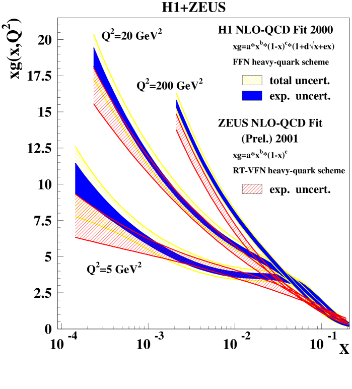
Figure 1: The gluon structure function in a proton measured at HERA.

Experimentally, an important increase of the number of gluons at small $x$ has indeed been observed in the Deep Inelastic Scattering experiments performed at HERA (see fig. 1), down to $x\sim 10^{-4}$. Such a growth raises a problem: if it were to continue to arbitrarily small $x$, it would induce an increase of hadronic cross-sections as a power of the center of mass energy, in violation of unitarity bounds.

However, as noticed by Gribov, Levin and Ryskin in [9], the BFKL equation includes only branching processes that increase the number of gluons ($g\to gg$ for instance), but not the recombination processes that could reduce the number of gluons (like $gg\to g$). While it may be legitimate to neglect the recombination process when the gluon density is small, this cannot remain so at arbitrarily high density: a saturation mechanism of some kind must set in. Treating the partons as ordinary particles, one can get a crude estimate of the onset of saturation from a simple mean free path argument. The recombination cross-section for gluon with transverse momentum $Q$ is roughly given by

$$\sigma\sim\frac{\alpha_{s}(Q^{2})}{Q^{2}}\;,$$ (1)

while the number of such gluons per unit of transverse area is given by

$$\rho\sim\frac{xG(x,Q^{2})}{\pi R^{2}}\;,$$ (2)

where $R$ is the radius of the hadron and $x$ the momentum fraction of the considered gluons. Saturation sets in when $\rho\sigma\sim 1$, or equivalently for:

$$Q^{2}=Q_{s}^{2}\;,\quad{\rm with\ }Q_{s}^{2}\sim\alpha_{s}(Q_{s}^{2})\frac{xG(x,Q_{s}^{2})}{\pi R^{2}}\;.$$ (3)

The momentum scale that characterizes this new regime, $Q_{s}$, is called the saturation momentum [10]. Partons with transverse momentum $Q>Q_{s}$ are in a dilute regime; those with $Q<Q_{s}$ are in the saturated regime.

A more refined argument for the onset of saturation was given in [11], where recombination is associated with a higher twist correction to the DGLAP equation. More generally, one may view the saturation momentum $Q_{s}$ as the scale at which QCD non linear effects become important. This occurs when field fluctuations are such that gluon kinetic energies become comparable to their interaction energies, that is when $\langle(\partial A)^{2}\rangle\sim\alpha_{s}\langle(A^{2})^{2}\rangle$, where $\langle A^{2}\rangle$ denotes the fluctuations of the gauge fields. Since the relevant dynamics is in the transverse plane, the magnitude of the gradient is fixed by the transverse momentum $Q$. As for the magnitude of the gauge field fluctuations, $\langle A^{2}\rangle$, they can be estimated from the particle number density in the transverse plane, i.e. $\langle A^{2}\rangle\sim\rho$, with $\rho$ given in eq. (2). The condition $\langle(\partial A)^{2}\rangle\sim\alpha_{s}\langle(A^{2})^{2}\rangle$ translates then into $Q^{2}\sim\alpha_{s}\langle A^{2}\rangle$, which is eq. (3) above. Note that at saturation, naive perturbation theory breaks down, even though $\alpha_{s}(Q_{s})$ may be small if $Q_{s}$ is large: the saturation regime is a regime of weak coupling, but large density.

Early estimates of $Q_{s}$ in nucleus-nucleus collisions were given in [12], and do not differ much from more modern ones [13]. But, as we have already emphasized, what has changed dramatically over the last decade is that we do not have only access to the boundary of the saturation region, we now have a complete dynamical picture of the saturation region. Before we turn to a short introduction to these new developments, let us indicate some expected characteristics of the saturated regime.

Note first that the saturation momentum increases as the gluon density increases. This may come from an increase of the gluon structure function as $x$ decreases. The increase of the density may also come from the coherent contributions of several nucleons in a nucleus. In large nuclei, one expects $Q_{s}^{2}\propto\alpha_{s}A^{1/3}$, where $A$ is the number of nucleons in the nucleus.

There is another feature. Consider the number of partons occupying a small disk of radius $1/Q_{s}$ in the transverse plane. This is easily estimated by combining eqs. (2) and (3); one finds this number to be proportional to $1/\alpha_{s}$. In such conditions of large numbers of quanta, classical field approximations may become relevant to describe the nuclear wave-functions.

3 Modern formulation:
the color glass condensate

Once one enters the saturated regime the evolution of the parton distributions can no longer be described by a linear equation such as the BFKL equation. One of the major breakthrough of the last ten years is that non linear equations have been obtained which allow us to follow the evolution of the partonic systems form the dilute regime to the dense, saturated, regime. These take different, equivalent, forms, generically referred to as the JIMWLK equation.

The color glass formalism, which provides the most complete physical picture, relies on the separation of the degrees of freedom in a high-energy hadron into frozen partons and dynamical fields, as discussed above. In the original McLerran and Venugopalan model [14, 15, 16], the fast partons are frozen, Lorentz contracted, color sources flying along the light-cone, and constitute a density of color charge $\rho({\boldsymbol{x}}_{\perp})$. Conversely, the low $x$ partons are described by classical gauge fields $A^{\mu}(x)$ determined by solving the Yang-Mills equations with the source given by the frozen partonic configuration. An average over all acceptable configurations must be performed.

The weight of a given configuration is a functional $W_{x_{0}}[\rho]$ of the density $\rho$ which depends on the separation scale $x_{0}$ between the modes which are described as frozen sources, and the modes which are described as dynamical fields. As one lowers this separation scale, more and more modes are included among the frozen sources, and therefore the functional $W_{x_{0}}$ evolves with $x_{0}$ according to a renormalization group equation [17, 18, 19, 20, 21, 22, 23, 24, 25, 26].

This evolution equation for $W_{x_{0}}[\rho]$ has been derived in [17, 18, 19, 20, 21, 22, 23, 24, 25, 26] and reads

$$\frac{\partial{W_{x_{0}}[\rho]}}{\partial\ln(1/x_{0})}=\frac{1}{2}\int_{\vec{{\boldsymbol{x}}}_{\perp},\vec{{\boldsymbol{y}}}_{\perp}}\frac{\delta}{\delta{\rho_{a}(\vec{{\boldsymbol{x}}}_{\perp})}}{\chi_{ab}(\vec{{\boldsymbol{x}}}_{\perp},\vec{{\boldsymbol{y}}}_{\perp})}\frac{\delta}{\delta\rho_{b}(\vec{{\boldsymbol{y}}}_{\perp})}{W_{x_{0}}[\rho]}\;,$$ (4)

where the kernel ${\chi_{ab}(\vec{{\boldsymbol{x}}}_{\perp},\vec{{\boldsymbol{y}}}_{\perp})}$ depends on the color density $\rho$ only via Wilson lines:

$$U({\boldsymbol{x}}_{\perp})\equiv{\cal P}\exp\left[-ig\int_{-\infty}^{+\infty}dz^{-}A^{+}(z^{-},{\boldsymbol{x}}_{\perp})\right]\;.$$ (5)

Here ${\cal P}$ denotes an ordering along the $x^{-}$ axis, $A^{+}$ is the classical color field of the hadron moving close to the speed of light in the $+z$ direction. The field $A^{+}$ depends implicitly on the frozen sources, i.e. on the color charge density $\rho({\boldsymbol{x}}_{\perp})$.

This functional evolution equation can be rewritten as an infinite hierarchy of equations for correlation functions of the $\rho$’s, or equivalently of the $U$’s. For instance, the correlator ${\rm tr}\big{<}U^{\dagger}({\boldsymbol{x}}_{\perp})U({\boldsymbol{y}}_{\perp})\big{>}$ of two Wilson lines has an evolution equation that involves a correlator of four Wilson lines. If one assumes that this 4-point correlator can be factored into a product of two 2-point functions, one obtains a closed equation for the 2-point function, called the Balitsky-Kovchegov [19, 21] equation:

$$\frac{\partial{\rm tr}\big{<}U^{\dagger}({\boldsymbol{x}}_{\perp})U({\boldsymbol{y}}_{\perp})\big{>}_{x_{0}}}{\partial\ln(1/x_{0})}=-\frac{\alpha_{s}}{2\pi^{2}}\int_{{\boldsymbol{z}}_{\perp}}\frac{({\boldsymbol{x}}_{\perp}-{\boldsymbol{y}}_{\perp})^{2}}{({\boldsymbol{x}}_{\perp}-{\boldsymbol{z}}_{\perp})^{2}({\boldsymbol{y}}_{\perp}-{\boldsymbol{z}}_{\perp})^{2}}$$

$$\times\Big{[}N_{c}{\rm tr}\big{<}U^{\dagger}({\boldsymbol{x}}_{\perp})U({\boldsymbol{y}}_{\perp})\big{>}_{x_{0}}-{\rm tr}\big{<}U^{\dagger}({\boldsymbol{x}}_{\perp})U({\boldsymbol{z}}_{\perp})\big{>}_{x_{0}}{\rm tr}\big{<}U^{\dagger}({\boldsymbol{z}}_{\perp})U({\boldsymbol{y}}_{\perp})\big{>}_{x_{0}}\Big{]}\;.$$ (6)

When the density of color charge $\rho$ is small, one can expand the Wilson line $U$ in powers of $\rho$. Eq. (6) becomes then a linear evolution equation for the correlator $\big{<}\rho({\boldsymbol{x}}_{\perp})\rho({\boldsymbol{y}}_{\perp})\big{>}_{x_{0}}$, or equivalently for the unintegrated gluon density, which is nothing but the BFKL equation.

The opposite limit, at very small $x_{0}$ (where the color charge density is large – far inside the saturation region), also leads to significant simplifications. Indeed, since the exponent in the Wilson lines is then a large quantity, one can use a Random Phase Approximation in which the correlators of Wilson lines are small. The solution is a Gaussian (albeit non-local in the transverse coordinates) [27]:

$$W_{x_{0}}[\rho]=\exp\Big{[}-\int_{{\boldsymbol{x}}_{\perp},{\boldsymbol{y}}_{\perp}}\frac{\rho({\boldsymbol{x}}_{\perp})\rho({\boldsymbol{y}}_{\perp})}{2\mu^{2}({\boldsymbol{x}}_{\perp}-{\boldsymbol{y}}_{\perp},x_{0})}\Big{]}\;.$$ (7)

This formula is not valid to arbitrarily short distances $|{\boldsymbol{x}}_{\perp}-{\boldsymbol{y}}_{\perp}|\to 0$, that is the domain of high $Q^{2}$ physics controlled by DGLAP evolution.

Like with the BFKL or DGLAP evolution equations, the initial condition for the evolution is truly a non-perturbative input. One can in principle try to model it, and then adjust the parameters of the model to fit experimental data. A simple model is that proposed by McLerran and Venugopalan, in which the initial $W_{x_{0}}[\rho]$ is a local Gaussian:

$$W_{x_{0}}[\rho]=\exp\Big{[}-\int_{{\boldsymbol{x}}_{\perp}}\frac{\rho({\boldsymbol{x}}_{\perp})\rho({\boldsymbol{x}}_{\perp})}{2\mu^{2}}\Big{]}\;.$$ (8)

At this point, one should stress that testing the predictions of the Color Glass Condensate in principle requires to test both the properties of the evolution with rapidity and the initial condition.

It is also important to note that the gaussians of eqs. (7) and (8) do not have the same status in the CGC framework: eq. (8) is one particular model for the initial condition at moderately small $x$, while eq. (7) is the asymptotic regime reached at very small $x$ regardless of the initial condition. The latter is therefore a property of the small $x$ evolution itself. The MV model requires an infrared cutoff at the scale $\Lambda_{{}_{QCD}}$. This is because assuming a truly local Gaussian distribution ignores the fact that color neutralization occurs on distance scales smaller than the nucleon size ($\sim\Lambda_{{}_{QCD}}^{-1}$): two $\rho$’s can only be uncorrelated if they are at transverse coordinates separated by at least the distance scale of color neutralization. In the asymptotic solution of eq. (7), there is no infrared problem because the color neutralization is built in the dependence of $\mu^{2}({\boldsymbol{x}}_{\perp}-{\boldsymbol{y}}_{\perp},x_{0})$ on the transverse coordinates. Color neutralization in fact occurs on distance scales of the order of $Q_{s}^{-1}(x_{0})$ [27]. This is the physical origin of the universality of the saturated regime.

4 Phenomenological predictions

4.1 Geometrical scaling

In the $(\ln(1/x),\ln(p_{\perp}))$ plane, the saturation domain is defined by the condition $\Lambda_{{}_{QCD}}\ll p_{\perp}\lesssim Q_{s}(x)$. In this region, one expects that observables (made dimensionless by scaling out the appropriate power of $p_{\perp}$) depending a priori on both $x$ and $p_{\perp}$ scale like functions of the unique variable $p_{\perp}/Q_{s}(x)$. This property is called “geometrical scaling” in the literature. It has been shown by Iancu, Itakura and McLerran in [28] that this scaling property holds in a much larger domain, whose upper bound is $p_{\perp}\lesssim Q_{s}(x)^{2}/\Lambda_{{}_{QCD}}$. This region has been labeled “extended scaling region” in figure 2.

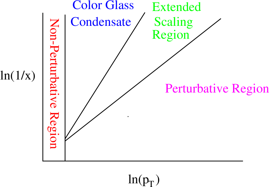
Figure 2: The scaling region in the $(\ln(1/x),\ln(p_{\perp}))$ plane.

Technically, the reason why this scaling survives outside of the saturation domain is that the (linear) BFKL equation that controls the evolution in $x$ when $p_{\perp}\gtrsim Q_{s}(x)$ preserves for a while the scaling properties inherited from the physics of the saturation region (which affects the BFKL evolution via a boundary condition at $p_{\perp}=Q_{s}(x)$).

Such a scaling has been searched for in the data of the DIS experiments at HERA, and it turns out that one can indeed represent all the small $x$ ($x<10^{-2}$) data points for the structure function $F_{2}(x,Q^{2})$ as a single function of the variable $\tau\equiv Q^{2}/Q_{s}^{2}(x)$ with

$$Q_{s}^{2}(x)\equiv Q_{0}^{2}\left(\frac{x_{0}}{x}\right)^{\lambda}\;.$$ (9)

This is illustrated by the plot of figure 3.

Figure 3: The $\gamma^{*}p$ cross-section at HERA, plotted against $\tau\equiv Q^{2}/Q_{s}^{2}(x)$.

The parameter $Q_{0}$ is set to $1$ GeV, while $x_{0}\approx 3.10^{-4}$ and $\lambda\approx 0.29$ are determined through a fit to the data [29]. By studying BFKL evolution to next-to-leading order, Triantafyllopoulos has obtained a value of $\lambda$ in good agreement with that observed [30].

4.2 Structure functions and diffraction in DIS

In an appropriate frame, and at leading order in $\alpha_{s}$, the cross section for the interaction of a virtual photon with a proton takes the following factorized form:

$$\sigma_{\gamma^{*}p}(x,Q^{2})=\int\limits_{0}^{1}dz\int d^{2}{\boldsymbol{r}}_{\perp}\left|\psi(Q^{2},z,{\boldsymbol{r}}_{\perp})\right|^{2}\sigma_{\rm dipole}(x,{\boldsymbol{r}}_{\perp})\;.$$ (10)

In this formula, $\psi(Q^{2},z,{\boldsymbol{r}}_{\perp})$ is the Fock component of the virtual photon light-cone wave function that corresponds to a $q\bar{q}$ dipole of size ${\boldsymbol{r}}_{\perp}$; it depends on the invariant mass $Q^{2}$ of the photon, on the transverse size ${\boldsymbol{r}}_{\perp}$ of the $q\bar{q}$ dipole, and on the fraction $z$ of the photon longitudinal momentum taken by the quark. The other factor in this formula, $\sigma_{\rm dipole}(x,{\boldsymbol{r}}_{\perp})$, is the total dipole-proton cross-section. It can be expressed in terms of a correlator of Wilson lines:

$$\sigma_{\rm dipole}(x,{\boldsymbol{r}}_{\perp})=\frac{2}{N_{c}}\int d^{2}{\boldsymbol{X}}_{\perp}{\rm tr}\,\left[1-\left<U({\boldsymbol{X}}_{\perp}+\frac{{\boldsymbol{r}}_{\perp}}{2})U^{\dagger}({\boldsymbol{X}}_{\perp}-\frac{{\boldsymbol{r}}_{\perp}}{2})\right>\right]\;,$$ (11)

where the average is taken over the color field of the proton.

Several models for this dipole cross-section have been used in the literature in order to fit HERA data. Golec-Biernat and Wüsthoff have used a very simple parameterization [31, 32]

$$\sigma_{\rm dipole}(x,{\boldsymbol{r}}_{\perp})=\sigma_{0}\left[1-e^{-\frac{1}{4}Q_{s}^{2}(x)r_{\perp}^{2}}\right],$$ (12)

which has led to good results for describing the data at $x<10^{-2}$ and moderate $Q^{2}$. In this formula, the scale $Q_{s}(x)$ was taken to be of the form given in eq. (9). This model fails however at large $Q^{2}$. This aspect was improved in [33], where the dipole cross-section is parameterized in a way that reproduces pQCD for small dipoles. Note that these approaches, even if they are inspired by saturation physics, do not derive the dipole cross-section from first principles. Recently, Iancu, Itakura and Munier [34] derived an expression of the dipole cross-section from the color glass condensate framework, and obtained a good fit of HERA data with a small number of free parameters. An equally good fit has been obtained by Gotsman, Levin, Lublinsky and Maor who derived the $x$ dependence of the dipole cross-section by solving numerically the BK equation and including DGLAP corrections [35].

One can express in a similarly factorized form the diffractive $\gamma^{*}p$ cross-section, where the exchange between the dipole and the target is color singlet. In fact, since the dipole cross-section involved in eqs. (10) and (11) is the total cross-section, one can use the optical theorem to deduce from it the forward elastic scattering amplitude:

$${\cal M}_{\rm elastic}(x,{\boldsymbol{r}}_{\perp},t=0)=\frac{i}{N_{c}}\int d^{2}{\boldsymbol{X}}_{\perp}{\rm tr}\,\left[1-\left<U({\boldsymbol{X}}_{\perp}+\frac{{\boldsymbol{r}}_{\perp}}{2})U^{\dagger}({\boldsymbol{X}}_{\perp}-\frac{{\boldsymbol{r}}_{\perp}}{2})\right>\right]\;,$$ (13)

assuming that this amplitude is predominantly imaginary. This can then be used to obtain for the diffractive DIS cross-section at $t=0$ an expression involving the square of the total dipole-proton cross-section:

$$\left.\frac{d\sigma^{{}^{D}}_{\gamma^{*}p}(x,Q^{2})}{dt}\right|_{t=0}=\frac{1}{16\pi}\int\limits_{0}^{1}dz\int d^{2}{\boldsymbol{r}}_{\perp}\left|\psi(Q^{2},z,{\boldsymbol{r}}_{\perp})\right|^{2}\sigma_{\rm dipole}^{2}(x,Q^{2})\;.$$ (14)

By using in this formula the total dipole cross-section fitted to the inclusive $F_{2}$, one obtains a good description of the measured diffractive DIS cross-section [31, 32]. Note however that keeping only the $q\bar{q}$ component of the photon wave function is a good approximation only when the invariant mass of the diffractively produced object is not too large. For large masses, one needs to consider also the $q\bar{q}g$ component.

4.3 Particle multiplicities at RHIC

In the framework of saturation models, predictions have been made for global observables like the total number of produced particles per unit of rapidity $dN/d\eta$. This can be studied as a function of the collision energy, the centrality of the collision, and the rapidity.

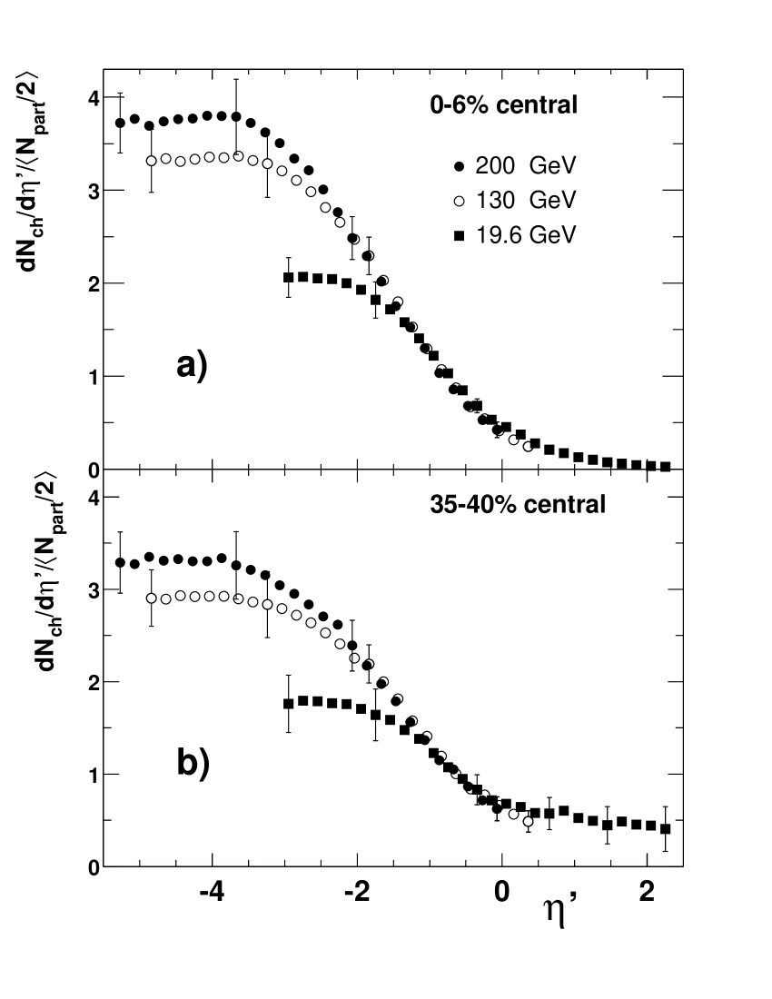
Figure 4: Particle multiplicity at RHIC for different collision energies, plotted against the rapidity of the produced particle relative to the rapidity of the beam $\eta^{\prime}\equiv\eta-\eta_{\rm beam}$ [36].

The Color Glass Condensate may provide a dynamical justification rooted in QCD for many general features of particles production in hadronic interactions. This may be the case in particular for the phenomenon of “limiting fragmentation”, i.e., the expectation that the rapidity distribution in the fragmentation region becomes independent of the collision energy at high energy. Evidence for such a behavior has indeed been observed by the PHOBOS collaboration, as is illustrated in figure 4. Here, one has plotted the rapidity distribution $dN/d\eta^{\prime}$ of produced particles in Au-Au collisions as a function of the rapidity relative to the incoming beam rapidity $\eta^{\prime}\equiv\eta-\eta_{\rm beam}$. When one increases the beam energy, one sees that $dN/d\eta^{\prime}$ is the same at large $\eta^{\prime}$ for all energies. The particles produced at some given (large) energy are those that would have been produced at lower energies plus new particles produced at a lower rapidity. An early interpretation of such a phenomenon in the language of the CGC has been proposed by Jalilian-Marian [37]. The interpretation suggested there is that in the fragmentation region of one of the nuclei ($\eta^{\prime}$ around zero), this nucleus is a dilute partonic system while the other nucleus is in a saturated state. The rise in multiplicity when one decreases $\eta^{\prime}$ is then attributed to the growth of the parton distribution in the dilute nucleus. One should emphasize however that no detailed quantitative analysis of the data presented in figure 4 has yet been done in this framework.

In comparing more quantitative predictions of the color glass formalism for $dN/d\eta$ to experimental data, it is important to keep the following points in mind. First, the color glass condensate can only predict the distribution of initial gluons, set free typically at a proper time $\tau\sim Q_{s}^{-1}$. Between this early stage and the final chemical freeze-out, the system undergoes several non-trivial steps: kinetic and chemical equilibration (possibly with additional parton production), hadronization, etc., which are most often ignored in calculations based on the color glass condensate. Secondly, even the calculation of the initial gluon production is a highly non-trivial task. It involves, in principle, solving the classical Yang-Mills equations in the presence of the color densities describing the distribution of frozen sources in both projectiles. This has been achieved analytically only for proton-nucleus collisions, when the color charge density inside the proton is assumed to be weak [38, 39, 40]. In the case of nucleus-nucleus collisions, two kinds of calculations have been performed:

(i) Ab initio numerical calculations [41, 42, 43, 44] that solve exactly the Yang-Mills equations for $AA$ collisions. The average over the color charge densities in the projectiles is performed by assuming that the distributions $W_{x_{0}}[\rho]$ are given by the MV model, i.e. by the gaussian of eq. (8). Quantum evolution effects are therefore not included. Note that when one calculates $dN/d\eta$ at $\eta=0$, the typical $x$ probed in the wave function of the nuclei is about $x\sim 10^{-2}$. Such calculations can therefore be used to test the validity of the gaussian model for $W_{x_{0}}[\rho]$ at $x_{0}\sim 10^{-2}$ as well as the non-linear dynamics of the classical field.

(ii) Approximate analytical calculations of the initial gluon spectrum [45]. These calculations assume $k_{\perp}$-factorization, although such a property is so far unproven for the collision of two dense projectiles.

     

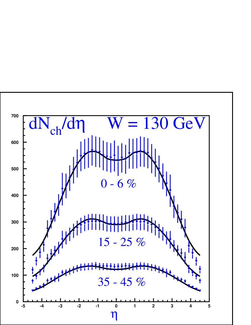
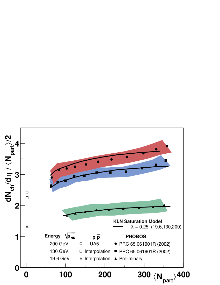
Figure 5: The number of particles per unit of rapidity in $AA$ collisions, as a function of rapidity for different centralities (left plot) and as a function of centrality at different energies (right plot). From [45] .

The non-integrated gluon distribution in the nuclei is taken to be of the form $\varphi(k_{\perp})\sim 1/\alpha_{s}$ for $k_{\perp}\ll Q_{s}(x)$ and $\varphi(k_{\perp})\sim Q_{s}^{2}(x)/k_{\perp}^{2}$ for $k_{\perp}\gg Q_{s}(x)$ (saturation appears through the fact that the gluon distribution does not diverge like $k_{\perp}^{-2}$ at small $k_{\perp}$). The rapidity dependence in this model is governed by that of $Q_{s}(x)$, eq. (9), where the exponent $\lambda$ can be taken from the study of the scaling properties in the HERA data. The overall normalization factor, as well as the value of $Q_{s}$ at a certain fixed energy, were fitted on RHIC data at $\sqrt{s}=130$ GeV. A prediction was then made in [45] for the value of $dN/d\eta$ at $\sqrt{s}=200$ GeV, which is in good agreement with experimental results, as illustrated in figure 5. One should also mention the fact that the value of $Q_{s}^{2}(x)$ one needs in this approach in order to reproduce the measured $dN/d\eta$, of the order of $2$ GeV², is relatively large compared to $\Lambda_{{}_{QCD}}$; this may perhaps be taken as an encouraging indication for the validity of the overall picture.

Note that the residual dependence on the number of participants in the quantity $N_{\rm part}^{-1}dN/d\eta$ calculated by Kharzeev, Levin and Nardi, comes entirely from the scale dependence of the strong coupling constant, as follows:

$$\frac{1}{N_{\rm part}}\frac{dN}{d\eta}\sim\frac{1}{\alpha_{s}(Q_{s}^{2})}\sim\ln(Q_{s}^{2}/\Lambda_{{}_{QCD}}^{2})\;.$$ (15)

However, strictly speaking, since the gluon multiplicity is obtained by solving the classical Yang-Mills equations, there is no running of $\alpha_{s}$ at this level of approximation. Certainly the running of $\alpha_{s}$ will come together with next-to-leading-order corrections, but it is at this point an ad hoc prescription. Since other interpretations of these same data, based on soft physics, are possible [46], it is unclear whether what we are “seeing” in the right hand panel of figure 5 is indeed the running of $\alpha_{s}(Q_{s}^{2})$ induced by the variation of the saturation scale with centrality.

     

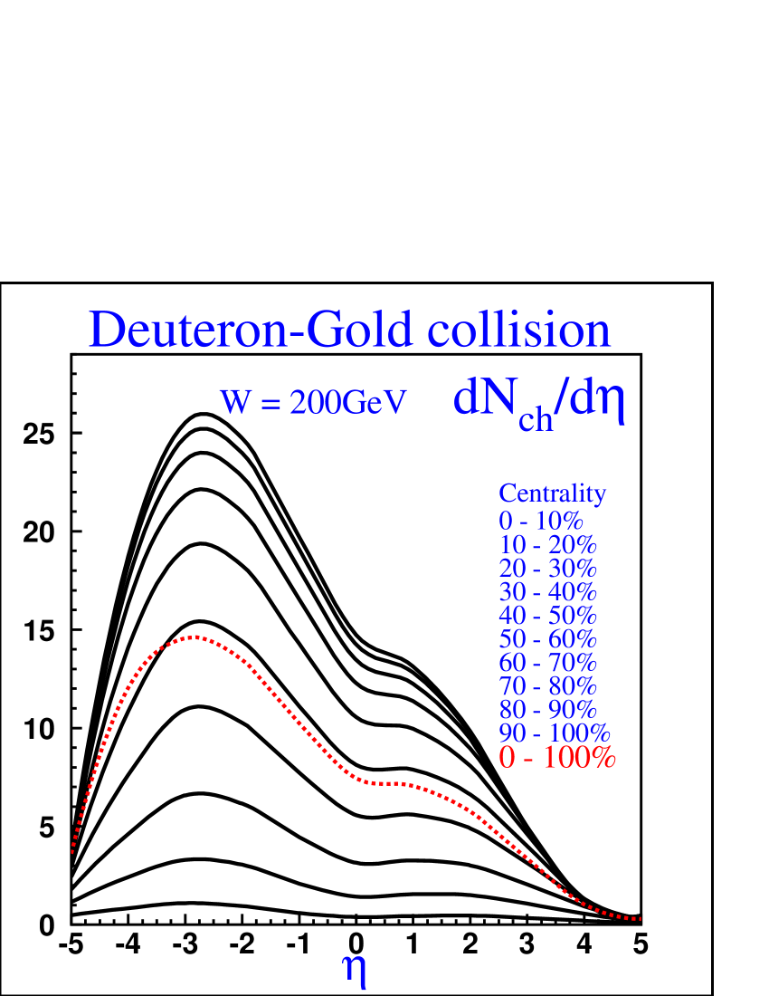
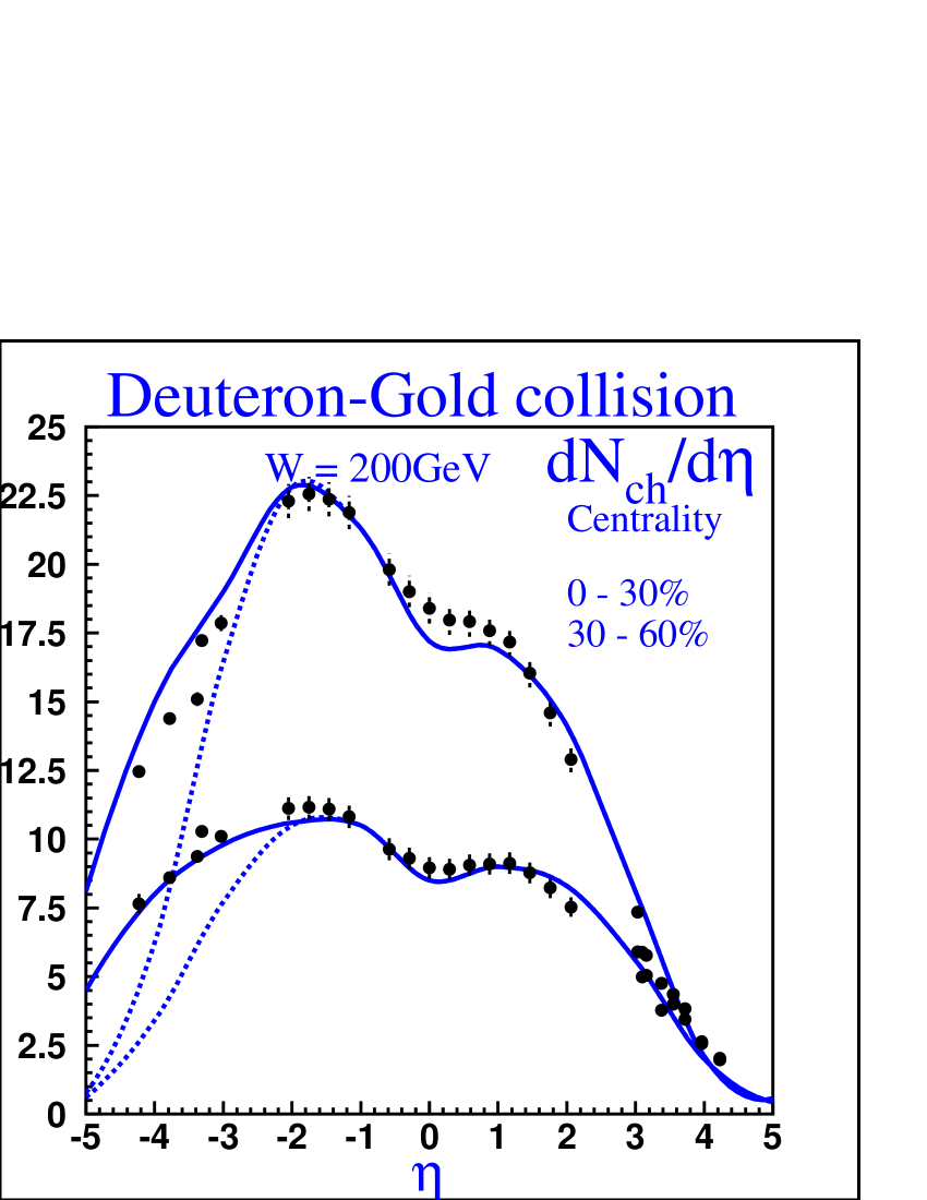
Figure 6: The number of particles per unit of rapidity in $dA$ collisions, as predicted in [47].

Such analysis of multiplicity distributions were extended to the case of deuteron-nucleus collisions [47], with results in fair agreement with RHIC data as illustrated in figure 6.

4.4 Spectra of produced particles

4.4.1 $p_{\perp}$ dependence

The saturation regime is characterized by a single scale, the saturation momentum $Q_{s}$, and as was the case for DIS, one may look for scaling laws in various observables. An attempt has been made to identify such a scaling in the transverse mass distributions of produced particles [48]: it has been found that the spectra for different species of particles are well represented by a single function of $m_{\perp}/Q_{s}$. The centrality dependence of the scaling parameter $Q_{s}^{2}$ was found in rough agreement with $Q_{s}^{2}\sim N_{\rm part}^{1/3}\sim A^{1/3}$. It should be emphasized however, that the hadrons whose spectra are measured have certainly undergone many reinteractions, so that their spectra are unlikely to reflect directly the initial momentum distribution of the color glass. Thus the interpretation of the $m_{\perp}$ scaling in the saturation picture is unconvincing.

In the case of deuteron-gold collisions, one does not expect final state interactions to play a dominant role. All the medium effects responsible for the difference between $pA$ and $pp$ collisions may in fact be taken into account in the color glass condensate. The produced partons hadronize then by the same mechanisms as in the vacuum, and their spectrum can be calculated by convoluting the partonic cross-section with the usual fragmentation functions. Moreover, since the calculation of the gluon spectrum only involves the correlator $\big{<}U(0)U^{\dagger}({\boldsymbol{x}}_{\perp})\big{>}$ [39, 49, 50, 40], one can in principle determine it from the dipole cross-section used in DIS [51]. A numerical calculation of the spectrum of hadrons produced in dA collisions has been performed in this approach in [52], with results in fairly good agreement with the spectrum measured at RHIC in $dA$ collisions.

The situation is far more complicated in the case of nucleus-nucleus collisions. Indeed, the gluons which emerge from the color glass shortly after the initial impact (typically at a proper time of the order of $Q_{s}^{-1}\sim 0.2$ fm) will interact strongly and may form a hot and dense medium (a quark-gluon plasma?). These interactions will presumably modify the gluon spectrum: the momentum distribution will become more isotropic and the hard tail of the spectrum will be suppressed by parton energy loss. These additional effects are not taken into account in the color glass, which merely provides the initial condition for the subsequent evolution of the system.

By assuming that local thermalization is achieved quickly, one can use hydrodynamics to describe this evolution. One may adjust the initial conditions so that averaged quantities like the local energy density match those predicted in saturation models. Such a strategy has been used by Hirano and Nara [53] as well as Eskola, Niemi, Ruuskanen and Rasanen [54, 55], who predicted hadron spectra in good agreement with the observed ones for $p_{\perp}\lesssim 2$ GeV. One should however keep in mind that this kind of test is by construction only sensitive to integrated quantities predicted by the CGC rather than to the detailed shape of the spectrum: indeed, the very assumption that thermalization occurs means that the system has lost memory of the initial momentum distribution except for the local energy density.

This remark implies that $dA$ collisions are certainly much better suited than $AA$ collisions in order to test the predictions of the color glass condensate, because the details of the system at early times are carried out to the final state almost unaltered. One should therefore be able to perform more direct tests of the CGC ideas in the context of $dA$ collisions.

4.4.2 Anisotropy

Another interesting quantity to look at is the so-called “elliptic flow”, which signals the existence of a significant pressure in the transverse direction [56], that converts the original spatial anisotropy into an anisotropy in momentum space.

This has been estimated by Krasnitz, Nara and Venugopalan [57] from the numerical solution of the classical Yang-Mills equations. The growth of the anisotropy with time is similar to what happens in hydrodynamical models, [57] and the full $v_{2}$ is attained after a time of the order of the size $R$ of the system. The $v_{2}$ obtained at late times in the color glass condensate framework is plotted in figure 7.

 

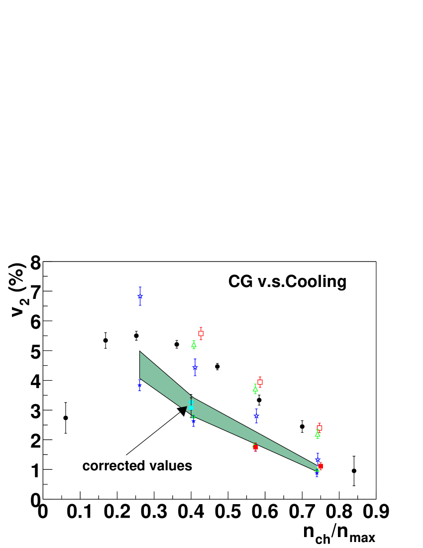
Figure 7: The centrality dependence of $v_{2}$ from the classical gluon production (green band). The black filled dots are STAR data.

One can see that although it is not in quantitative agreement with the data, it has the correct order of magnitude and reproduces qualitatively the dependence on the multiplicity (i.e. on the centrality). However, the dependence of $v_{2}$ on the transverse momentum is in clear disagreement with the RHIC data: the color glass condensate predicts that $v_{2}$ has a maximum at small momentum and then falls to zero at large momentum, while the measured $v_{2}$ increases monotonously up $p_{\perp}\sim 2$ GeV and remains almost constant at higher momenta. Note that the description of the system in terms of classical fields breaks down for times that are large compared to $Q_{s}^{-1}$, that is for times needed to establish the $v_{2}$. It is nevertheless instructive to see that this model, which does not rely on the assumption of thermalization, produces a $v_{2}$ of comparable magnitude to the $v_{2}$ obtained in hydrodynamical expansion over similar time-scales.

4.5 Ratios of spectra: $R_{AA}$, $R_{dA}$

The comparison of the $p_{\perp}$ spectra in $AA$ or $dA$ to the corresponding ones in $pp$ collisions is usually done through the following ratio:

$$R_{AA}\equiv\frac{\left.\frac{dN}{dyd^{2}{\boldsymbol{p}}_{\perp}}\right|_{AA}}{N_{\rm coll}\left.\frac{dN}{dyd^{2}{\boldsymbol{p}}_{\perp}}\right|_{pp}}\;,\quad R_{dA}\equiv\frac{\left.\frac{dN}{dyd^{2}{\boldsymbol{p}}_{\perp}}\right|_{dA}}{N_{\rm coll}\left.\frac{dN}{dyd^{2}{\boldsymbol{p}}_{\perp}}\right|_{pp}}\;,$$ (16)

where $N_{\rm coll}$ is the number of binary collisions. For the production of high $p_{\perp}$ particles, expected to scale like the number of binary collisions, these ratios should be unity. These ratios have been measured at RHIC both for $AA$ and $dA$ collisions.

 

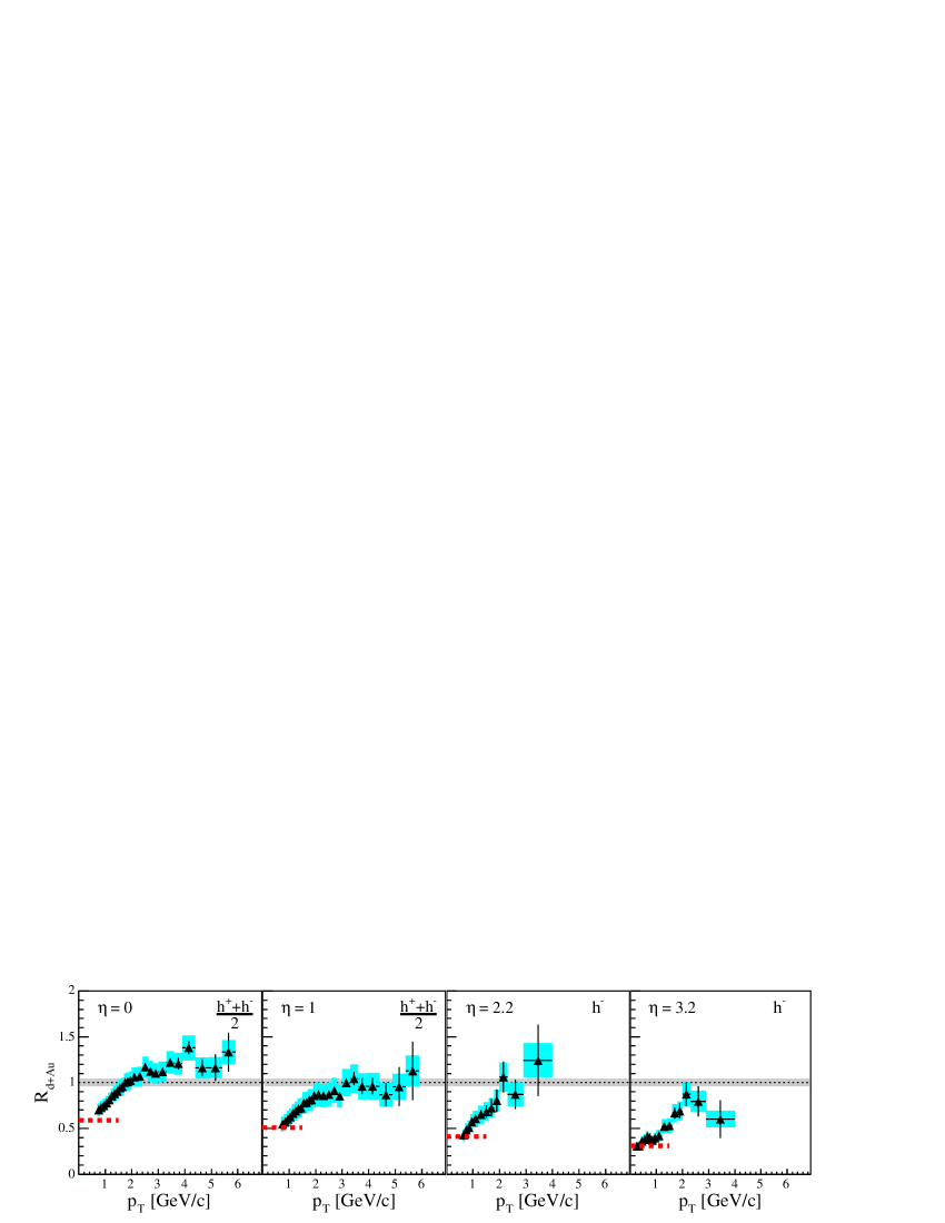
Figure 8: The ratio $R_{dA}$ measured at RHIC by the BRAHMS collaboration at several rapidities (positive rapidities correspond to the fragmentation region of the deuteron) [58].

In $AA$ collisions at central rapidity ($\eta=0$), the measured $R_{AA}$ is much smaller than one (around $0.2$) in central collisions, even at $p_{\perp}$’s as high as $10$ GeV, and approaches one from below as one goes to more and more peripheral collisions. However, at the values of $x$ probed by gluon production at mid-rapidity ($x\sim 10^{-2}$ for $p_{\perp}\sim 1$ GeV), where one expects the distribution $W_{x_{0}}[\rho]$ to be given by the McLerran-Venugopalan model (eq. (8)), the $R_{AA}$ predicted in the color glass condensate at a time of the order of $Q_{s}^{-1}$ has a maximum larger than $1$ at small $p_{\perp}$ and then goes to one from above as $p_{\perp}$ increases [59]. This maximum of $R_{AA}$ in the MV model is interpreted as a manifestation of the multiple (elastic) rescatterings of the produced gluon, which tend to redistribute the $p_{\perp}$ spectrum by depleting the small $p_{\perp}$’s and enhancing the high $p_{\perp}$’s (Cronin effect). The observed suppression of $R_{AA}$ therefore requires final state effects, and is naturally interpreted as energy loss ([60, 61, 62, 63, 64], see also [65] for a recent review) of the high $p_{\perp}$ partons as they go through the dense medium formed in $AA$ collisions.

At much smaller values of $x$, which can be probed by looking at particle production at large rapidity, one expects the distribution $W_{x_{0}}[\rho]$ to reach the asymptotic form of eq. (7). It has been found that with such a distribution of color sources, the color glass condensate leads to a suppression of the ratios $R_{AA}$ or $R_{dA}$ [66] (see the plots of figure 9, taken from [67]). However, in order to disentangle this suppression which is an initial state effect (because it comes from the “wave function” of the projectiles) from the energy loss, one needs an experiment in which one has no significant final state effects, like $dA$ collisions. The ratio $R_{dA}$ measured by the BRAHMS experiment is shown in figure 8 [58]. One can see at $\eta=0$ a very different behavior than for $AA$ collisions: the ratio $R_{dA}$ has a maximum above one and seems to go to one from above at high $p_{\perp}$. As one increases the rapidity of the observed particles, one can see the ratio $R_{dA}$ drop very fast and eventually become consistently smaller than one. Such a behavior with rapidity was predicted in [67] (see the figure 9), where the evolution of the ratio $R_{dA}$ was evaluated by evolving the unintegrated gluon distribution in a nucleus using the Balitsky-Kovchegov equation, starting from the McLerran-Venugopalan model at large $x$.

 

Figure 9: Evolution of the ratios $R_{AA}$ and $R_{dA}$ with rapidity in the color glass condensate framework. The initial condition is the McLerran-Venugopalan model. Note that the calculation of $R_{AA}$ assumed $k_{\perp}$-factorization.

Similar qualitative results were also obtained in [68], in [69] within a toy model for the gluon distribution inspired from the color glass condensate, and in [40] where the two distributions of frozen sources given in eqs. (7) and (8) were used in order to compute the ratio $R_{dA}$. The onset of the suppression of the ratio $R_{dA}$ as one increases the rapidity was studied analytically in [70], where it was shown that the rapid suppression seems to be due to the fact that the gluon distribution evolves faster in a proton than it does in a nucleus, because the nucleus reaches the saturation regime earlier. Recently, a more quantitative study of this effect has been performed in [71]. So far, the color glass condensate is the only framework in which one reproduces, at least qualitatively, both the the Cronin effect at central rapidities and its suppression at forward rapidities.

5 Discussion and outlook

Considerable theoretical progress has been made over the last ten years in understanding the physics that govern the wave function of a hadron at high energy. Not only has one acquired a fairly intuitive picture that is universally applicable to all hadrons at high energy, but an operational framework has been developed in which many phenomena can be described quantitatively. One is now in principle able to study and make predictions in the entire $x,k_{\perp}$ plane (with the exception of the truly non-perturbative region $k_{\perp}\lesssim\Lambda_{{}_{QCD}}$), with non-perturbative physics entering only as an initial condition for otherwise known evolution equations.

With the realization that the characteristic scale that governs high energy hadronic interactions, the saturation momentum $Q_{s}$, is enhanced by the size of the projectiles in collisions involving nuclei, RHIC can be viewed as a place of choice in order to test these ideas and confront them to data. And indeed the phenomenology based on saturation physics has been quite successful in describing what is observed at RHIC. Whenever relevant comparisons with data can be made (global observables in $AA$ collisions, spectra in $dA$ collisions), the tests are successful. In cases of marked disagreement, like with the elliptic flow, one understands that the discrepancy comes from using the color glass picture beyond its domain of applicability.

One may ask whether the predictions which have been tested so far are distinctive features of the color glass condensate that cannot be reasonably explained by other models. Naturally, the more precise the question, the more discriminatory the answer. Because in $AA$ collisions the final state interactions are important, only global observables are preserved from early times to the final state. Therefore $AA$ collisions are in general not ideal for direct tests of the color glass condensate (many global features of $AA$ collisions are present in any reasonable model of hadronic interactions, and thus not characteristic of the color glass condensate). Collisions involving a small projectile, like $dA$ collisions, where effects of final state interactions can be minimized, at least in some kinematical domains, are much better suited. And indeed the suppression of the ratio $R_{dA}$ at forward rapidities could turn out to be such a distinctive measurement, since no other model has been able so far to provide a natural explanation of what is observed. This is also one instance where non trivial quantum evolution could be playing a significant role. What is missing for this to become a real test is a detailed calculation of this effect that would go beyond the many qualitative approaches performed so far. Clearly, doing such calculations, as well as getting more precise data, is of utmost importance.

From comparisons with data, one has also learned that final state interactions are generally very important in $AA$ collisions, and many observables do not simply reflect the properties of the partonic system produced in the early stages. The color glass condensate only provides the initial condition for a subsequent evolution of the system leading possibly to the formation of a quark-gluon plasma. Understanding whether and how thermalization happens presents interesting theoretical challenges (see [72, 73, 74, 75, 76] for some recent works on the subject) and is of utmost importance for giving a solid theoretical basis to present descriptions of $AA$ collisions.

As a final remark, oriented towards the future, one may note that many of the phenomena uncovered at RHIC, should become more clearly visible at the LHC. There, with center of mass energies of $5.5~{}$TeV for $AA$ collisions, the typical value of $x$ at mid-rapidity will be about $5.10^{-4}$ and values as small as $10^{-5}$ could be reached at forward rapidities. This corresponds roughly to values of $Q_{s}^{2}$ ranging from $5~{}$GeV² to $14$ GeV². Such large values of the saturation momentum make the coupling constant $\alpha_{s}$ smaller than at RHIC, giving firmer grounds to the weak coupling expansion used in the color glass condensate framework. A corollary of this is that the gluon occupation number in the saturation region will be larger, making the classical description also more justified.

References

- [1] R.P. Feynman, Photon-Hadron Interactions, Frontiers in Physics, W.A. Benjamin, (1972).
- [2] J.D. Bjorken, Lecture Notes in Physics, 56, Springer, Berlin (1976).
- [3] E.A. Kuraev, L.N. Lipatov, V.S. Fadin, Sov. Phys. JETP 45, 199 (1977).
- [4] I. Balitsky, L.N. Lipatov, Sov. J. Nucl. Phys. 28, 822 (1978).
- [5] V.N. Gribov, L.N. Lipatov, Sov. J. Nucl. Phys. 15, 438 (1972).
- [6] V.N. Gribov, L.N. Lipatov, Sov. J. Nucl. Phys. 15, 675 (1972).
- [7] G. Altarelli, G. Parisi, Nucl. Phys. B 126, 298 (1977).
- [8] Yu. Dokshitzer, Sov. Phys. JETP 46, 641 (1977).
- [9] L.V. Gribov, E.M. Levin, M.G. Ryskin, Phys. Rept. 100, 1 (1983).
- [10] A.H. Mueller, Nucl. Phys. B 558, 285 (1999).
- [11] A.H. Mueller, J-W. Qiu, Nucl. Phys. B 268, 427 (1986).
- [12] J.P. Blaizot, A.H. Mueller, Nucl. Phys. B 289, 847 (1987).
- [13] A.H. Mueller, Talk given at QM2002, Nantes, France, July 2002, Nucl. Phys. A 715, 20 (2003).
- [14] L.D. McLerran, R. Venugopalan, Phys. Rev. D 49, 2233 (1994).
- [15] L.D. McLerran, R. Venugopalan, Phys. Rev. D 49, 3352 (1994).
- [16] L.D. McLerran, R. Venugopalan, Phys. Rev. D 50, 2225 (1994).
- [17] J. Jalilian-Marian, A. Kovner, A. Leonidov, H. Weigert, Nucl. Phys. B 504, 415 (1997).
- [18] J. Jalilian-Marian, A. Kovner, A. Leonidov, H. Weigert, Phys. Rev. D 59, 014014 (1999).
- [19] I. Balitsky, Nucl. Phys. B 463, 99 (1996).
- [20] Yu.V. Kovchegov, Phys. Rev. D 54, 5463 (1996).
- [21] Yu.V. Kovchegov, Phys. Rev. D 61, 074018 (2000).
- [22] J. Jalilian-Marian, A. Kovner, L.D. McLerran, H. Weigert, Phys. Rev. D 55, 5414 (1997).
- [23] E. Iancu, A. Leonidov, L.D. McLerran, Nucl. Phys. A 692, 583 (2001).
- [24] E. Iancu, A. Leonidov, L.D. McLerran, Phys. Lett. B 510, 133 (2001).
- [25] H. Weigert, Nucl. Phys. A 703, 823 (2002).
- [26] E. Ferreiro, E. Iancu, A. Leonidov, L.D. McLerran, Nucl. Phys. A 703, 489 (2002).
- [27] E. Iancu, K. Itakura, L.D. McLerran, Nucl. Phys. A 724, 181 (2003).
- [28] E. Iancu, K. Itakura, L.D. McLerran, Nucl. Phys. A 708, 327 (2002).
- [29] A.M. Stasto, K. Golec-Biernat, J. Kwiecinski, Phys. Rev. Lett. 86, 596 (2001).
- [30] D.N. Triantafyllopoulos, Nucl. Phys. B 648, 293 (2003).
- [31] K. Golec-Biernat, M. Wüsthoff, Phys. Rev. D 59, 014017 (1999).
- [32] K. Golec-Biernat, M. Wüsthoff, Phys. Rev. D 60, 114023 (1999).
- [33] J. Bartels, K. Golec-Biernat, H. Kowalski, Phys. Rev. D 66, 014001 (2002).
- [34] E. Iancu, K. Itakura, S. Munier, hep-ph/0310338.
- [35] E. Gotsman, E. Levin, M. Lublinsky, U. Maor, Eur. Phys. J. C 27, 411 (2003).
- [36] B.B. Back, et al., PHOBOS collaboration, Phys. Rev. Lett. 91, 052303 (2003).
- [37] J. Jalilian-Marian, nucl-th/0212018.
- [38] Yu.V. Kovchegov, A.H. Mueller, Nucl. Phys. B 529, 451 (1998).
- [39] A. Dumitru, L.D. McLerran, Nucl. Phys. A 700, 492 (2002).
- [40] J.P. Blaizot, F. Gelis, R. Venugopalan, hep-ph/0402256.
- [41] A. Krasnitz, R. Venugopalan, Phys. Rev. Lett. 84, 4309 (2000).
- [42] A. Krasnitz, R. Venugopalan, Phys. Rev. Lett. 86, 1717 (2001).
- [43] A. Krasnitz, Y. Nara, R. Venugopalan, Phys. Rev. Lett. 87, 192302 (2001).
- [44] T. Lappi, Phys. Rev. C 67, 054903 (2003).
- [45] D. Kharzeev, E. Levin, Phys. Lett. B 523, 79 (2001).
- [46] A. Capella, D. Sousa, Phys. Lett. B 511, 185 (2001).
- [47] D. Kharzeev, E. Levin, M. Nardi, Nucl. Phys. A 730, 448 (2004).
- [48] J. Schaffner-Bielich, D. Kharzeev, L.D. McLerran, R. Venugopalan, Nucl. Phys. A 705, 494 (2002).
- [49] A. Dumitru, J. Jalilian-Marian, Phys. Rev. Lett. 89, 022301 (2002).
- [50] A. Dumitru, J. Jalilian-Marian, Phys. Lett. B 547, 15 (2002).
- [51] F. Gelis, J. Jalilian-Marian, Phys. Rev. D 67, 074019 (2003).
- [52] J. Jalilian-Marian, nucl-th/0402080.
- [53] T. Hirano, Y. Nara, nucl-th/0404039.
- [54] K.J. Eskola, H. Niemi, P.V. Ruuskanen, S.S. Rasanen, Phys. Lett. B 566, 187 (2003).
- [55] K.J. Eskola, H. Niemi, P.V. Ruuskanen, S.S. Rasanen, Talk at Quark Matter 2002, Nantes, France, 18-24 Jul 2002, Nucl. Phys. A 715, 561 (2003).
- [56] J.Y. Ollitrault, Phys. Rev. D 46, 229 (1992).
- [57] A. Krasnitz, Y. Nara, R. Venugopalan, Phys. Lett. B 554, 21 (2003).
- [58] I. Arsene, et al., BRAHMS collaboration, nucl-ex/0403005.
- [59] J. Jalilian-Marian, Y. Nara, R. Venugopalan, Phys. Lett. B 577, 54 (2003).
- [60] J.D. Bjorken, FERMILAB-PUB-82-059-THY (1982).
- [61] X.N. Wang, M. Gyulassy, Phys. Rev. Lett. 68, 1480 (1992).
- [62] M. Gyulassy, X.N. Wang, Nucl. Phys. B 420, 583 (1994).
- [63] R. Baier, Y.L. Dokshitzer, S. Peigné, D. Schiff, Phys. Lett. B 345, 277 (1995).
- [64] R. Baier, Y.L. Dokshitzer, A.H. Mueller, S. Peigné, D. Schiff, Nucl. Phys. B 483, 291 (1997).
- [65] M. Gyulassy, I. Vitev, X.N. Wang, B.N. Zhang, QGP 3, edited by R.C. Hwa and X.N. Wang, World Scientific, Singapore, nucl-th/0302077.
- [66] D. Kharzeev, E. Levin, L.D. McLerran, Phys. Lett. B 561, 93 (2003).
- [67] J.L. Albacete, N. Armesto, A. Kovner, C.A. Salgado, U.A. Wiedemann, hep-ph/0307179.
- [68] R. Baier, A. Kovner, U.A. Wiedemann, Phys. Rev. D 68, 054009 (2003).
- [69] D. Kharzeev, Yu. Kovchegov, K. Tuchin, Phys. Rev. D 68, 094013 (2003).
- [70] E. Iancu, K. Itakura, D. Triantafyllopoulos, hep-ph/0403103.
- [71] D. Kharzeev, Yu. Kovchegov, K. Tuchin, hep-ph/0405045.
- [72] R. Baier, A.H. Mueller, D. Schiff, D. Son, Phys. Lett. B 502, 51 (2001).
- [73] P. Romatschke, M. Strickland, Phys. Rev. D 68, 036004 (2003).
- [74] S. Mrowczynski, A. Rebhan, M. Strickland, hep-ph/0403256.
- [75] P. Arnold, J. Lenaghan, G.D. Moore, JHEP 0308, 002 (2003).
- [76] J. Berges, S. Borsanyi, C. Wetterich, hep-ph/0403234.