Resonance estimates for single spin asymmetries in elastic electron-nucleon scattering

Abstract

We discuss the target and beam normal spin asymmetries in elastic electron-nucleon scattering which depend on the imaginary part of two-photon exchange processes between electron and nucleon. We express this imaginary part as a phase space integral over the doubly virtual Compton scattering tensor on the nucleon. We use unitarity to model the doubly virtual Compton scattering tensor in the resonance region in terms of $\gamma^{*}N\to\pi N$ electroabsorption amplitudes. Taking those amplitudes from a phenomenological analysis of pion electroproduction observables, we present results for beam and target normal single spin asymmetries for elastic electron-nucleon scattering for beam energies below 1 GeV and in the 1-3 GeV region, where several experiments are performed or are in progress.

I Introduction

Elastic electron-nucleon scattering in the one-photon exchange approximation is a time-honoured tool to access information on the structure of hadrons. Experiments with increasing precision have become possible in recent years, mainly triggered by new techniques to perform polarization experiments at the electron scattering facilities. This has allowed to reach a new frontier in the measurement of hadron structure quantities, such as its electroweak form factors, parity violating effects, nucleon polarizabilities, $N\to\Delta$ transition form factors, or the measurement of spin dependent structure functions, to name a few. For example, experiments using polarized electron beams and measuring the ratio of the recoil nucleon in-plane polarization components have profoundly extended our understanding of the nucleon electromagnetic form factors. For the proton, such polarization experiments which access the ratio $G_{Ep}/G_{Mp}$ of the proton’s electric ( $G_{Ep}$ ) to magnetic ( $G_{Mp}$ ) form factors have been performed out to a momentum transfer $Q^{2}$ of 5.6 GeV² Jones00 ; Gayou02 . It came as a surprise that these experiments extracted a ratio of $G_{Ep}/G_{Mp}$ which is clearly at variance with unpolarized measurements Slac94 ; Chr04 ; Arr03 using the Rosenbluth separation technique.
The understanding of this puzzle has generated a lot of activity recently, and is a prerequisite to use electron scattering as a precision tool. It has been suggested on general grounds in Ref. GV03 that this puzzle may be explained by a two-photon exchange amplitude of the level of a few percent. The resulting failure of the one-photon exchange approximation to unpolarized elastic electron-nucleon scattering can be understood from the observation that $G_{Mp}$ and $G_{Ep}$ enter quadratically in the unpolarized cross section. It turns out that $G_{Ep}^{2}$ may become a small quantity compared with $G_{Mp}^{2}$, and is further suppressed by a kinematical factor $\sim 1/Q^{2}$. Therefore, it becomes increasingly difficult to extract this term at larger momentum transfer. Already at moderate momentum transfers, the weight of the term proportional to $G_{E}^{2}$ drops at the 1 % level and one may expect that correction terms due to two-photon exchange become competitive and eventually dominate over the $G_{E}^{2}$ term. The polarization transfer method on the other hand is much less affected because it directly measures the ratio of $G_{Ep}/G_{Mp}$ , i.e. depends linearly on $G_{E}$.
Recently, several model calculations of the $2\gamma$ exchange amplitude have been performed. In Ref. BMT03 , a calculation of the $2\gamma$ exchange when the hadronic intermediate state is a nucleon was performed. It found that the $2\gamma$ exchange correction with intermediate nucleon can partially resolve the discrepancy between the two experimental techniques. Recently, the $2\gamma$ exchange contribution to elastic electron-nucleon scattering has been estimated at large momentum transfer YCC04 , through the scattering off a parton in a proton by relating the process on the nucleon to the generalized parton distributions. This calculation found that the $2\gamma$ exchange contribution is indeed able to quantitatively resolve the existing discrepancy between Rosenbluth and polarization transfer experiments.
To push the precision frontier further in electron scattering, one needs a good control of $2\gamma$ exchange mechanisms and needs to understand how they may or may not affect different observables. This justifies a systematic study of such $2\gamma$ exchange effects, both theoretically and experimentally. The real (dispersive) part of the $2\gamma$ exchange amplitude can be accessed through the difference between elastic electron and positron scattering off a nucleon. The imaginary (absorptive) part of the $2\gamma$ exchange amplitude on the other hand can be accessed through a single spin asymmetry (SSA) in elastic electron-nucleon scattering, when either the target or beam spin are polarized normal to the scattering plane, as has been discussed some time ago in Ref. RKR71 . As time reversal invariance forces this SSA to vanish for one-photon exchange, it is of order $\alpha=e^{2}/(4\pi)\simeq 1/137$. Furthermore, to polarize an ultra-relativistic particle in the direction normal to its momentum involves a suppression factor $m/E$ (with $m$ the mass and $E$ the energy of the particle), which typically is of order $10^{-4}-10^{-3}$ when the electron beam energy is in the 1 GeV range. Therefore, the resulting target normal SSA can be expected to be of order $10^{-2}$, whereas the beam normal SSA is of order $10^{-6}-10^{-5}$. A measurement of such small asymmetries is quite demanding experimentally. However, in the case of a polarized lepton beam, asymmetries of the order ppm are currently accessible in parity violation (PV) elastic electron-nucleon scattering experiments. The parity violating asymmetry involves a beam spin polarized along its momentum. However the SSA for an electron beam spin normal to the scattering plane can also be measured using the same experimental set-ups. First measurements of this beam normal SSA at beam energies below 1 GeV have yielded values around 10 ppm Wells01 ; Maas03 . At higher beam energies, the beam normal SSA can also be measured in upcoming PV elastic electron-nucleon scattering experiments Happex ; G0 ; E158 .
First estimates of the target normal SSA in elastic electron-nucleon scattering have been performed in Refs. RKR71 ; RKR73 . In those works, the $2\gamma$ exchange with nucleon intermediate state (so-called elastic or nucleon pole contribution) has been calculated, and the inelastic contribution has been estimated in a very forward angle approximation. Estimates within this approximation have also been reported for the beam normal SSA in Ref. AAM02 . Recently, the general formalism for elastic electron-nucleon scattering with lepton helicity flip, which is needed to describe the beam normal SSA, has been developed in Ref. GGV04 . Furthermore, the beam normal SSA has also been estimated at large momentum transfers $Q^{2}$ in Ref. GGV04 using a parton model, which was found crucial YCC04 to interpret the results from unpolarized electron-nucleon elastic scattering, as discussed before. In the handbag model of Refs. YCC04 ; GGV04 , the corresponding $2\gamma$ exchange amplitude has been expressed in terms of generalized parton distributions, and the real and imaginary part of the $2\gamma$ exchange amplitude are related through a dispersion relation. Hence in the partonic regime, a direct comparison of the imaginary part with experiment can provide a very valuable cross-check on the calculated result for the real part.
To use the elastic electron-nucleon scattering at low momentum transfer as a high precision tool, such as in present day PV experiments, one may also want to quantify the $2\gamma$ exchange amplitude. To this aim, one may envisage a dispersion formalism for the elastic electron-nucleon scattering amplitudes, as has been discussed some time ago in the literature BPB87 . To develop this formalism, the necessary first step is a precise knowledge of the imaginary part of the two-photon exchange amplitude, which enters in both the beam and target normal SSA. The study of this imaginary part of the $2\gamma$ exchange is the subject of this paper. Using unitarity, one can relate the imaginary part of the $2\gamma$ amplitude to the electroabsorption amplitudes on a nucleon. When measuring the imaginary part of the elastic electron-nucleon amplitude through a normal SSA at sufficiently low energies, below or around two-pion production threshold, one is in a regime where these electroproduction amplitudes are relatively well known using pion electroproduction experiments as input. One strategy is therefore to investigate this new tool of beam and target normal SSA first in the region where one has a good first knowledge of the imaginary part of the $2\gamma$ exchange. As both photons in the $2\gamma$ exchange process are virtual and integrated over, an observable such as the beam or target normal SSA is sensitive to the electroproduction amplitudes on the nucleon for a range of photon virtualities. This may provide information on resonance transition form factors complementary to the information obtained from current pion electroproduction experiments.
Finally, by understanding the $2\gamma$ exchange contributions for the case of electromagnetic electron-nucleon scattering, one may extend this calculation to electroweak processes, where the $\gamma Z$ and $W^{+}W^{-}$ box diagrams are in several cases the leading unknown contributions entering in electroweak precision experiments.
We start by briefly reviewing the elastic electron-nucleon scattering formalism beyond the one-photon exchange approximation in Section II, and discuss the target and beam normal spin asymmetries in Section III. Subsequently, we study the imaginary part of the two-photon exchange amplitudes in Section IV. We express this imaginary part as a phase space integral over the doubly virtual Compton scattering tensor on the nucleon. In Section V, we use unitarity to model the doubly virtual Compton scattering tensor in the resonance region in terms of $\gamma^{*}N\to\pi N$ electroabsorption amplitudes. We take those amplitudes from a state-of-the-art phenomenological analysis (MAID Dre99 ) of pion electroproduction observables. In Section VI, we show our results for beam and target normal SSA for beam energies below 1 GeV and in the 1-3 GeV region, where several experiments at MIT-Bates, MAMI and Jefferson Lab (JLab) are performed or in progress. Our conclusions and an outlook are given in Section VII.

II Elastic electron-nucleon scattering beyond the one-photon exchange approximation

In this section, we briefly review the elastic electron-nucleon scattering formalism beyond the one-photon exchange approximation, as has been developed recently in Refs. GV03 ; GGV04 . For the kinematics of elastic electron-nucleon scattering :

$$e^{-}(k)+N(p)\rightarrow e^{-}(k^{\prime})+N(p^{\prime}),$$ (1)

we adopt the usual definitions :

$$P=\frac{p+p^{\prime}}{2},\,K=\frac{k+k^{\prime}}{2},\,q=k-k^{\prime}=p^{\prime}-p,$$ (2)

and choose

$$Q^{2}=-q^{2},\,\nu=K.P,$$ (3)

as the independent invariants of the scattering. The invariant $\nu$ is related to the polarization parameter $\varepsilon$ of the virtual photon, which can be expressed as (neglecting the electron mass) :

$$\varepsilon=\frac{\nu^{2}-M^{4}\tau(1+\tau)}{\nu^{2}+M^{4}\tau(1+\tau)},$$ (4)

where $M$ is the nucleon mass.
For a theory which respects Lorentz, parity and charge conjugation invariance, the general amplitude for elastic scattering of two spin 1/2 particles can be expressed by 6 independent helicity amplitudes or equivalently by six invariant amplitudes. The total amplitude can be decomposed in general in terms of a lepton spin non-flip and spin flip part :

$$T\;=\;T_{non-flip}\;+\;T_{flip}.$$ (5)

The non-flip amplitude which conserves the helicity of the electron (in the limit $m_{e}=0$) depends upon 3 invariant amplitudes, and has been parametrized in Ref. GV03 as :

$$T_{non-flip}\, = \,\frac{e^{2}}{Q^{2}}\,\bar{u}(k^{\prime})\gamma_{\mu}u(k)\,\cdot\,\bar{u}(p^{\prime})\left(\tilde{G}_{M}\,\gamma^{\mu}-\tilde{F}_{2}\frac{P^{\mu}}{M}+\tilde{F}_{3}\frac{\gamma.KP^{\mu}}{M^{2}}\right)u(p).$$ (6)

The amplitude which flips the electron helicity (i.e. is of the order of the mass of the electron, $m_{e}$), depends on 3 additional invariants which have been introduced in Ref. GGV04 as :

$$T_{flip}\, = \,\frac{m_{e}}{M}\,\frac{e^{2}}{Q^{2}}\left[\,\bar{u}(k^{\prime})u(k)\,\cdot\,\bar{u}(p^{\prime})\left(\tilde{F}_{4}\,+\tilde{F}_{5}\frac{\gamma.K}{M}\right)u(p)\,+\,\tilde{F}_{6}\,\bar{u}(k^{\prime})\gamma_{5}u(k)\,\cdot\,\bar{u}(p^{\prime})\gamma_{5}u(p)\right].$$ (7)

In Eqs. (6,7), $\tilde{G}_{M}$, $\tilde{F}_{2}$, $\tilde{F}_{3}$, $\tilde{F}_{4}$, $\tilde{F}_{5}$, $\tilde{F}_{6}$ are complex functions of $\nu$ and $Q^{2}$, and the factor $e^{2}/Q^{2}$ has been introduced for convenience. Furthermore in Eq. (7), we extracted an explicit factor $m_{e}/M$ out of the amplitudes, which reflects the fact that for a vector interaction (such as in QED), the electron helicity flip amplitude vanishes when $m_{e}\to 0$. In the Born approximation, one obtains :

$$\tilde{G}_{M}^{Born}(\nu,Q^{2})\, = \,G_{M}(Q^{2}),$$

$$\tilde{F}_{2}^{Born}(\nu,Q^{2})\, = \,F_{2}(Q^{2}),$$

$$\tilde{F}_{3,\,4,\,5,\,6}^{Born}(\nu,Q^{2})\, = \,0,$$ (8)

where $G_{M}(F_{2})$ are the proton magnetic (Pauli) form factors respectively. The invariant amplitude $\tilde{F}_{2}$ can be traded for $\tilde{G}_{E}$, defined as :

$$\tilde{G}_{E}\equiv\tilde{G}_{M}-(1+\tau)\tilde{F}_{2},$$ (9)

which has the property that in the Born approximation it reduces to the electric form factor, i.e.

$$\tilde{G}^{Born}_{E}(\nu,Q^{2})=G_{E}(Q^{2}).$$ (10)

To separate the one- and two-photon exchange contributions, it is then useful to introduce the decompositions :

$$\tilde{G}_{M}\, = \,G_{M}+\delta\tilde{G}_{M},$$ (11)

$$\tilde{G}_{E}\, = \,G_{E}+\delta\tilde{G}_{E}.$$ (12)

Since the amplitudes $\delta\tilde{G}_{M}$, $\delta\tilde{G}_{E}$, $\tilde{F}_{3}$, $\tilde{F}_{4}$, $\tilde{F}_{5}$, and $\tilde{F}_{6}$ vanish in Born approximation, they must originate from processes involving at least the exchange of two photons. Relative to the factor $e^{2}$ introduced in Eqs. (6, 7), we see that they are of order $e^{2}.$

III Single spin asymmetries in elastic electron-nucleon scattering

An observable which is directly proportional to the two- (or multi-) photon exchange is given by the elastic scattering of an unpolarized electron on a proton target polarized normal to the scattering plane (or the recoil polarization normal to the scattering plane, which is exactly the same assuming time-reversal invariance). For a target polarized perpendicular to the scattering plane, the corresponding single spin asymmetry, which we refer to as the target normal spin asymmetry ($A_{n}$), is defined by :

$$A_{n}\,=\,\frac{\sigma_{\uparrow}-\sigma_{\downarrow}}{\sigma_{\uparrow}+\sigma_{\downarrow}}\,,$$ (13)

where $\sigma_{\uparrow}$ ($\sigma_{\downarrow}$) denotes the cross section for an unpolarized beam and for a nucleon spin parallel (anti-parallel) to the normal polarization vector, defined as :

$$S_{n}^{\mu}\,=\,(\,0\,,\,\vec{S}_{n}\,),\hskip 56.9055pt\vec{S}_{n}\,\equiv\,(\vec{k}\times\vec{k}^{\prime})\,/\,|\vec{k}\times\vec{k}^{\prime}|.$$ (14)

As has been shown by de Rujula et al. RKR71 , the target (or recoil) normal spin asymmetry is related to the absorptive part of the elastic $eN$ scattering amplitude (see Section IV). Since the one-photon exchange amplitude is purely real, the leading contribution to $A_{n}$ is of order $O(e^{2})$, and is due to an interference between one- and two-photon exchange amplitudes.
When neglecting terms which correspond with electron helicity flip (i.e. setting $m_{e}=0$), $A_{n}$ can be expressed in terms of the invariants for electron-nucleon elastic scattering, defined in Eqs. (6, 7), as YCC04  :

$$A_{n} = \sqrt{\frac{2\,\varepsilon\,(1+\varepsilon)}{\tau}}\,\,\left(G_{M}^{2}\,+\,\frac{\varepsilon}{\tau}\,G_{E}^{2}\right)^{-1}$$ (15)

$$\times \left\{-\,G_{M}\,{\cal I}\left(\delta\tilde{G}_{E}+\frac{\nu}{M^{2}}\tilde{F}_{3}\right)\,+\,G_{E}\,{\cal I}\left(\delta\tilde{G}_{M}+\left(\frac{2\varepsilon}{1+\varepsilon}\right)\frac{\nu}{M^{2}}\tilde{F}_{3}\right)\right\}$$

$$+ {\mathcal{O}}(e^{4}),$$

where $\cal I$ denotes the imaginary part.
For a beam polarized perpendicular to the scattering plane, we can also define a single spin asymmetry, analogously as in Eq. (13), where now $\sigma_{\uparrow}$ ($\sigma_{\downarrow}$) denotes the cross section for an unpolarized target and for an electron beam spin parallel (anti-parallel) to the normal polarization vector, given by Eq. (14). We refer to this asymmetry as the beam normal spin asymmetry ($B_{n}$). It explicitly vanishes when $m_{e}=0$ as it involves an electron helicity flip. Using the general electron-nucleon scattering amplitude of Eqs. (6,7), $B_{n}$ is given by GGV04  :

$$B_{n}\, = \,\frac{2\,m_{e}}{Q}\,\sqrt{2\,\varepsilon\,(1-\varepsilon)}\,\sqrt{1+\frac{1}{\tau}}\,\left(G_{M}^{2}\,+\,\frac{\varepsilon}{\tau}\,G_{E}^{2}\right)^{-1}$$

$$\times \left\{-\tau\,G_{M}\,{\mathcal{I}}\left(\tilde{F}_{3}+\frac{1}{1+\tau}\,\frac{\nu}{M^{2}}\,\tilde{F}_{5}\right)\,-\,G_{E}\,{\mathcal{I}}\left(\tilde{F}_{4}+\frac{1}{1+\tau}\,\frac{\nu}{M^{2}}\,\tilde{F}_{5}\right)\right\}$$

$$+ \,{\mathcal{O}}(e^{4}),$$ (16)

As for $A_{n}$, we immediately see that $B_{n}$ vanishes in the Born approximation, and is therefore of order $e^{2}$.

IV Imaginary (absorptive) part of the two-photon exchange amplitude

In this section we relate the imaginary part of the two-photon exchange amplitude to the absorptive part of the doubly virtual Compton scattering tensor on the nucleon, as shown in Fig. 1. In the following we consider the helicity amplitudes for the elastic electron-nucleon scattering, defined in the $e^{-}N$ $c.m.$ frame, which are denoted by $T(h^{\prime},\lambda_{N}^{\prime}\,;\,h,\lambda_{N})$. Here $h(h^{\prime})$ denote the helicities of the initial (final) electrons and $\lambda_{N}(\lambda_{N}^{\prime})$ denote the helicities of the initial (final) nucleons. These helicity amplitudes can be expressed in terms of the invariant amplitudes introduced in Eqs. (6,7), and the corresponding relations can be found in Appendix A. These relations allow us to calculate the invariant amplitudes, once we have constructed a model for the helicity amplitudes.

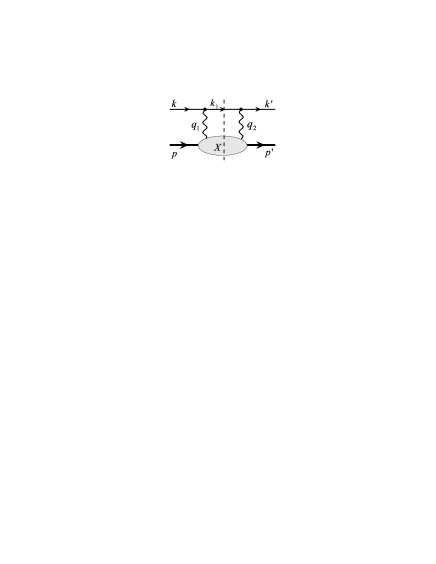
Figure 1: The two-photon exchange diagram. The filled blob represents the response of the nucleon to the scattering of the virtual photon.

We start by calculating the discontinuity of the two-photon exchange amplitude, shown in Fig. 1, which is given by

$${\rm Abs}\,T_{2\gamma}\;=\;e^{4}\int\frac{d^{3}\vec{k}_{1}}{(2\pi)^{3}2E_{k_{1}}}\bar{u}(k^{\prime},h^{\prime})\gamma_{\mu}(\gamma\cdot k_{1}+m_{e})\gamma_{\nu}u(k,h)\frac{1}{Q_{1}^{2}Q_{2}^{2}}\cdot W^{\mu\nu}(p^{\prime},\lambda_{N}^{\prime};p,\lambda_{N})\,,$$ (17)

where the momenta are defined as indicated on Fig. 1, with $q_{1}\equiv k-k_{1}$, $q_{2}\equiv k^{\prime}-k_{1}$, and $q_{1}-q_{2}=q$. Denoting the c.m. angle between initial and final electrons as $\theta_{c.m.}$, the momentum transfer $Q^{2}\equiv-q^{2}$ in the elastic scattering process can be expressed as :

$$Q^{2}=\frac{(s-M^{2})^{2}}{2\,s}\,\left(1-\cos\theta_{c.m.}\right)\,+\,{\mathcal{O}}(m_{e}^{2}),$$ (18)

with $s=(k+p)^{2}$. Furthermore, $Q_{1}^{2}\equiv-q_{1}^{2}=-(k-k_{1})^{2}$ and $Q_{2}^{2}\equiv-q_{2}^{2}=-(k^{\prime}-k_{1})^{2}$ correspond with the virtualities of the two spacelike photons.
In Eq. (17), the hadronic tensor $W^{\mu\nu}(p^{\prime},\lambda_{N}^{\prime};p,\lambda_{N})$ corresponds with the absorptive part of the doubly virtual Compton scattering tensor with two space-like photons :

$$W^{\mu\nu}(p^{\prime},\lambda_{N}^{\prime};p,\lambda_{N})\;=\;\sum_{X}\,(2\pi)^{4}\,\delta^{4}(p+q_{1}-p_{X})<p^{\prime}\,\lambda_{N}^{\prime}|J^{\dagger\mu}(0)|X>\,<X|J^{\nu}(0)|p\,\lambda_{N}>\,,$$ (19)

where the sum goes over all possible on-shell intermediate hadronic states $X$. Note that in the limit $p^{\prime}=p$, Eq. (19) reduces to the forward tensor for inclusive electron-nucleon scattering and can be parametrized by the usual 4 nucleon forward structure functions. In the non-forward case however, the absorptive part of the doubly virtual Compton scattering tensor of Eq. (19) which enters in the evaluation of target and beam normal spin asymmetries, depends upon 18 invariant amplitudes Tar75 . Though this may seem as a forbiddingly large number of new functions, we may use the unitarity relation to express the full non-forward tensor in terms of electroproduction amplitudes $\gamma^{*}N\to X$. The number of intermediate states $X$ which one considers in the calculation will then put a limit on how high in energy one can reliably calculate the hadronic tensor Eq. (19). In the following section, we will model the tensor $W^{\mu\nu}$ for the elastic contribution ($X=N$), and in the resonance region as a sum over all $\pi N$ intermediate states (i.e. $X=\pi N$), using a phenomenological state-of-the-art calculation for the $\gamma^{*}N\to\pi N$ amplitudes.
The phase space integral in Eq. (17) runs over the 3-momentum of the intermediate (on-shell) electron. Evaluating the process in the $e^{-}N$ c.m. system, we can express the c.m. momentum of the intermediate electron as :

$$|\vec{k}_{1}|^{2}\, = \,\frac{(s-W^{2}+m_{e}^{2})^{2}\,-\,4sm_{e}^{2}}{4s}$$ (20)

$$\simeq \frac{(s-W^{2})^{2}}{4s}\left\{1-2\,m_{e}^{2}\,\frac{(s+W^{2})}{(s-W^{2})^{2}}\right\}\,+\,{\mathcal{O}}(m_{e}^{4}),$$

where $W^{2}\equiv p_{X}^{2}$ is the squared invariant mass of the intermediate state $X$. The c.m. momentum $|\vec{k}|$ of the initial (and final) electrons is given by the analogous expression as Eq. (20) by replacing $W^{2}\to M^{2}$. The three-dimensional phase space integral in Eq. (17) depends, besides the magnitude $|\vec{k}_{1}|$, upon the solid angle of the intermediate electron. We define the polar c.m. angle $\theta_{1}$ of the intermediate electron w.r.t. to the direction of the initial electron. The azimuthal angle $\phi_{1}$ is chosen such that $\phi_{1}=0$ corresponds with the scattering plane of the $eN\to eN$ process. Having defined the kinematics of the intermediate electron, we can express the virtuality of both exchanged photons. The virtuality of the photon with four-momentum $q_{1}$ is given by :

$$Q_{1}^{2} \simeq\frac{1}{2\,s}\,\left\{(s-M^{2})\,(s-W^{2})\,(1-\cos\theta_{1})\right.$$

$$\left.-m_{e}^{2}(s+W^{2})\left(1-\frac{(s-M^{2})}{(s-W^{2})}\cos\theta_{1}\right)-m_{e}^{2}(s+M^{2})\left(1-\frac{(s-W^{2})}{(s-M^{2})}\cos\theta_{1}\right)\right\}\,+\,{\mathcal{O}}(m_{e}^{4}).$$

The virtuality $Q_{2}^{2}$ of the second photon has an analogous expression as Eq. (IV) by replacing $\cos\theta_{1}$ by $\cos\theta_{2}$, where $\theta_{2}$ is the angle between the intermediate and final electrons. In terms of the polar and azimuthal angles $\theta_{1}$ and $\phi_{1}$ of the intermediate electron, one can express :

$$\cos\theta_{2}\,=\,\sin\theta_{c.m.}\,\sin\theta_{1}\,\cos\phi_{1}\,+\,\cos\theta_{c.m.}\,\cos\theta_{1}.$$ (22)

In case the intermediate electron is collinear with the initial electron (i.e. for $\theta_{1}\to 0$, $\phi_{1}\to 0$), one obtains from Eq. (IV) that both photon virtualities are given by :

$$Q_{1,\,VCS}^{2}\, \equiv \,Q_{1}^{2}(\theta_{1}=0,\phi_{1}=0)\,\simeq\,m_{e}^{2}\,\frac{(W^{2}-M^{2})^{2}}{(s-W^{2})\,(s-M^{2})},$$

$$Q_{2,\,VCS}^{2}\, \equiv \,Q_{2}^{2}(\theta_{1}=0,\phi_{1}=0)\,\simeq\,\frac{(s-W^{2})}{(s-M^{2})}\,Q^{2}\,+\,{\mathcal{O}}(m_{e}^{2}).$$ (23)

Note that when the intermediate and initial electrons are collinear, then also the photon with momentum $\vec{q}_{1}=\vec{k}-\vec{k}_{1}$ is collinear with this direction. For the elastic case ($W=M$) this precisely corresponds with the situation where the first photon is soft (i.e. $q_{1}\to 0$) and where the second photon carries the full momentum transfer $Q_{2}^{2}\simeq Q^{2}$. For the inelastic case ($W>M$) the first photon is hard but becomes quasi-real (i.e. $Q_{1}^{2}\sim m_{e}^{2}$). In this case, the virtuality of the second photon is smaller than $Q^{2}$. An analogous situation occurs when the intermediate electron is collinear with the final electron (i.e. $\theta_{2}\to 0$, $\phi_{1}\to 0$, which is equivalent with $\theta_{1}\to\theta_{c.m.}$). These kinematical situations with one quasi-real photon and one virtual photon correspond with quasi virtual Compton scattering (quasi-VCS), and correspond at the lepton side with the Bethe-Heitler process, see e.g. Ref. GV98 for details.
Besides the near singularities corresponding with quasi-VCS, where the intermediate electron is collinear with either the incoming or outgoing electrons, the two photon exchange process also has a near singularity when the intermediate electron momentum goes to zero $|\vec{k}_{1}|\to 0$ (i.e. the intermediate electron is soft). In this case the first photon takes on the full momentum of the initial electron, i.e. $\vec{q}_{1}\to\vec{k}$, whereas the second photon takes on the full momentum of the final electron, i.e. $\vec{q}_{2}\to\vec{k}^{\prime}$. One immediately sees from Eq. (20) that this situation occurs when the invariant mass of the hadronic state takes on its maximal value $W_{max}=\sqrt{s}-m_{e}$. In this case, both photon virtualities are given by :

$$Q_{1,\,RCS}^{2}\,=\,Q_{2,\,RCS}^{2}\,\simeq\,m_{e}\,\frac{(s-M^{2})}{\sqrt{s}}\,\left(1-\cos\theta_{1}\right).$$ (24)

This kinematical situation with two quasi-real photons corresponds with quasi-real Compton scattering (quasi-RCS).
Due to the near singularities in the phase space integral of Eq. (17) corresponding with the quasi-VCS and quasi-RCS processes, special care was taken when integrating over these regions, as the integrand varies strongly over regions governed by the electron mass. Below we will show that these near singularities may give important contributions (logarithmic enhancements) under some kinematical conditions. In Fig. 2, we show the full kinematical accessible region for the virtualities $Q_{1}^{2},Q_{2}^{2}$ in the phase space integral of Eq. (17).

Figure 2: Kinematical accessible region for the virtualities $Q_{1}^{2},Q_{2}^{2}$ in the phase space integral of Eqs. (17) and (26), for MAMI (left panels) and JLab (right panels) kinematics for different c.m. angles $\theta_{c.m.}$ as indicated on the ellipses. The accessible regions correspond with the inside of the ellipses and are shown both for the elastic (upper panels) and for inelastic (lower panels) intermediate hadronic states. The intersection with the axes correspond with quasi-VCS, whereas the situation at $W=\sqrt{s}-m_{e}$ where all ellipses shrink to the point $Q_{1}^{2}=Q_{2}^{2}\simeq 0$ corresponds with quasi-RCS.

The normal spin asymmetries $A_{n}$ and $B_{n}$, discussed in Sections III, are a direct measure of the absorptive part of the two-photon exchange amplitude and can be expressed as RKR71  :

$$A_{n}\;=\;\frac{2\,{\rm Im}(\sum_{spins}T_{1\gamma}^{*}\cdot{\rm Abs}\,T_{2\gamma})}{\sum_{spins}|T_{1\gamma}|^{2}}\,,$$ (25)

where $T_{1\gamma}$ denotes the one-photon exchange amplitude. Using Eq. (17), we can express Eq. (25) in terms of a 3-dimensional phase-space integral :

$$A_{n}\;=\;-\frac{1}{(2\pi)^{3}}\frac{e^{2}Q^{2}}{D(s,Q^{2})}\int_{M^{2}}^{(\sqrt{s}-m_{e})^{2}}dW^{2}\,\frac{|\vec{k}_{1}|}{4\,\sqrt{s}}\int d\Omega_{k_{1}}\frac{1}{Q_{1}^{2}\,Q_{2}^{2}}\,{\rm Im}\left\{L_{\alpha\mu\nu}\,H^{\alpha\mu\nu}\right\}\,.$$ (26)

The denominator factor $D(s,Q^{2})$ in Eq. (26) is given through the one-photon exchange cross section as :

$$D(s,Q^{2})\;\equiv\;\frac{Q^{4}}{e^{4}}\cdot\sum_{spins}|T_{1\gamma}|^{2}\,=\,\,8\,\,\frac{(4M^{2}\tau)^{2}}{1-\varepsilon}\,\,\left\{\,G_{M}^{2}\,+\,\frac{\varepsilon}{\tau}\,G_{E}^{2}\,\right\}.$$ (27)

Furthermore in Eq. (26), the leptonic ($L_{\alpha\mu\nu}$) and hadronic ($H^{\alpha\mu\nu}$) tensors are given by :

$$L_{\alpha\mu\nu} = \bar{u}(k^{\prime},h^{\prime})\gamma_{\mu}(\gamma\cdot k_{1}+m_{e})\gamma_{\nu}u(k,h)\cdot\left[\bar{u}(k^{\prime},h^{\prime})\gamma_{\alpha}u(k,h)\right]^{*}\,,$$ (28)

$$H^{\alpha\mu\nu} = W^{\mu\nu}\cdot\left[\bar{u}(p^{\prime},\lambda_{N}^{\prime})\Gamma^{\alpha}(p^{\prime},p)u(p,\lambda_{N})\right]^{*}\,,$$ (29)

where

$$\Gamma^{\alpha}(p^{\prime},p)\equiv G_{M}\gamma^{\alpha}-F_{2}\,P^{\alpha}/M.$$ (30)

In Eqs. (28, 29) a sum is understood over the helicities of the unpolarized particles. To evaluate the target normal spin asymmetry $A_{n}$, we need the unpolarized lepton tensor, which is given by (neglecting the terms proportional to the electron mass $m_{e}$) :

$$L_{\alpha\mu\nu}^{unpol} = \mathrm{Tr}\left\{/{k^{\prime}}\gamma_{\mu}/{k_{1}}\gamma_{\nu}/{k}\gamma_{\alpha}\right\}.$$ (31)

The beam normal spin asymmetry $B_{n}$ involves the polarized lepton tensor, which is given by :

$$L_{\alpha\mu\nu}^{pol} = \mathrm{Tr}\left\{(/{k^{\prime}}+m_{e})\gamma_{\mu}(/{k_{1}}+m_{e})\gamma_{\nu}\gamma_{5}/{\xi}(/{k}+m_{e})\gamma_{\alpha}\right\},$$ (32)

where $\xi^{\beta}$ is the polarization vector, for an electron polarized normal to the scattering plane. We see from Eq. (32) that the polarized lepton tensor vanishes for massless electrons. Keeping only the leading term in $m_{e}$, it is given by :

$$L_{\alpha\mu\nu}^{pol} = m_{e}\left\{\,-\mathrm{Tr}\left\{\gamma_{5}\gamma_{\mu}/{k_{1}}\gamma_{\nu}/{\xi}/{k}\gamma_{\alpha}\right\}+\mathrm{Tr}\left\{\gamma_{5}/{k^{\prime}}\gamma_{\mu}/{k_{1}}\gamma_{\nu}/{\xi}\gamma_{\alpha}\right\}-\mathrm{Tr}\left\{\gamma_{5}/{k^{\prime}}\gamma_{\mu}\gamma_{\nu}/{\xi}/{k}\gamma_{\alpha}\right\}\,\right\}$$ (33)

$$+ \,{\mathcal{O}}(m_{e}^{2}).$$

V Models for the hadronic tensor

In this section, we discuss several models for the non-forward hadronic tensor $W^{\mu\nu}$ of Eq. (19) which enters in the imaginary part of the two-photon exchange amplitude. These models will be used further on to evaluate the target and beam normal spin asymmetries.
An initial guess, is to approximate the non-forward tensor by the corresponding forward tensor in terms of 4 nucleon structure functions, as was done in the calculations of Ref. RKR71 , and adapted in Ref. AAM02 by complementing the nucleon structure functions by a form factor dependence. This may be a reliable first estimate when one is interested in the kinematical limit of high energy and very small momentum transfer ($Q^{2}\ll s$), corresponding with the Regge regime. The SLAC E158 experiment E158 , which corresponds with $E_{\gamma}\simeq 50$ GeV and $Q^{2}\leq 0.05$ GeV², accesses this diffractive region and may be a good testing ground for such models.
To go beyond the very forward angle approximation for the hadronic tensor, and in order to compare quantitatively with beam normal spin asymmetry measurements performed or in progress at MIT-Bates Wells01 , MAMI Maas03 , and JLab Happex ; G0 at intermediate beam energies in the 1 GeV region, one immediately faces the full complexity of the non-forward doubly virtual Compton scattering tensor. This non-forward tensor can be parametrized in general in terms of 18 invariant amplitudes Tar75 . As we are interested in this work in the absorptive part of the non-forward doubly virtual Compton scattering tensor, we may use the unitarity relation to express the full non-forward tensor in terms of electroabsorption amplitudes $\gamma^{*}N\to X$ at different photon virtualities. This same strategy has been used before in the description of real and virtual Compton scattering in the resonance region, and checked against data in Ref. DPV03 . We will subsequently model the non-forward tensor $W^{\mu\nu}$ for the elastic contribution ($X=N$), and in the resonance region as a sum over all $\pi N$ intermediate states (i.e. $X=\pi N$).

V.1 Elastic contribution

The elastic contribution to $W^{\mu\nu}$, corresponding with the nucleon intermediate state in the blob of Fig. 1, is exactly calculable in terms of on-shell nucleon electromagnetic form factors as :

$$W^{\mu\nu}_{el}(p^{\prime},\lambda_{N}^{\prime};p,\lambda_{N})\; = \;2\pi\,\delta(W^{2}-M^{2})$$ (34)

$$\times \,\bar{u}(p^{\prime},\lambda_{N}^{\prime})\,\Gamma^{\mu}(p^{\prime},p_{X})\,(\gamma\cdot p_{X}+M)\,\Gamma^{\nu}(p_{X},p)\,u(p,\lambda_{N})\,,$$

where $\Gamma^{\mu}$ is given as in Eq. (30).

V.2 Inelastic contribution : sum over $\pi N$ intermediate states using the MAID model (resonance region)

The inelastic contribution to $W^{\mu\nu}$ corresponding with the $\pi N$ intermediate states in the blob of Fig. 1, is given by

$$W^{\mu\nu}(p^{\prime},\lambda^{\prime}_{N};p,\lambda_{N}) = \frac{1}{4\pi^{2}}\frac{|\vec{p}_{\pi}|^{2}}{[|\vec{p}_{\pi}|(E_{\pi}+E_{n})+E_{\pi}|\vec{k}_{1}|\hat{k}_{1}\cdot\hat{p}_{\pi}]}$$ (35)

$$\times\sum_{\lambda_{n}}\int{\rm d}\Omega_{\pi}\;\bar{u}(p^{\prime},\lambda^{\prime}_{N})J^{\dagger\mu}_{\pi N}u(p_{n},\lambda_{n})\;\bar{u}(p_{n},\lambda_{n})J^{\nu}_{\pi N}u(p,\lambda_{N}),$$

where $p_{\pi}=(E_{\pi},\vec{p}_{\pi})$ and $p_{n}=(E_{n},\vec{p}\,_{n})$ are the four-momenta of the intermediate pion and nucleon states respectively, and $\vec{k}_{1}=-\vec{p}_{\pi}-\vec{p}_{n}$. In Eq. (35) the integration runs over the polar and azimuthal angles of the intermediate pion, and $J^{\nu}_{\pi N}$ and $J^{\dagger\mu}_{\pi N}$ are the pion electroproduction currents, describing the excitation and de-excitation of the $\pi N$ intermediate state, respectively. Following Ref. Ber67 , we parametrize the matrix element of the pion electroproduction current in terms of six invariant amplitudes $A_{i}$ as :

$$\bar{u}(p_{n},\lambda_{n})\,J^{\nu}_{\pi N}\,u(p,\lambda_{N})=8\pi W\,\,\bar{u}(p_{n},\lambda_{n})\sum_{i=1}^{6}A_{i}(W^{2},t_{\pi},Q_{1}^{2})\,M^{\nu}_{i}\,u(p,\lambda_{N}),$$ (36)

where $W^{2}=(p+q_{1})^{2}=(p_{\pi}+p_{n})^{2}$ is the squared c.m. energy of the $\pi N$ system, $t_{\pi}=(p-p_{n})^{2}=(p_{\pi}-q_{1})^{2}$ is the squared four-momentum transfer in the $\gamma N\to\pi N$ process. In Eq. (36), the covariants $M^{\nu}_{i}$ are given by

$$M^{\nu}_{1} = -\frac{1}{2}i\gamma_{5}\left(\gamma^{\nu}/{q}_{1}-/{q}_{1}\gamma^{\nu}\right)\,,$$

$$M^{\nu}_{2} = 2i\gamma_{5}\left(P_{in}^{\nu}\,q_{1}\cdot(p_{\pi}-\frac{1}{2}q_{1})-(p_{\pi}-\frac{1}{2}q_{1})^{\nu}q_{1}\cdot P_{in}\right)\,,$$

$$M^{\nu}_{3} = -i\gamma_{5}\left(\gamma^{\nu}\,q_{1}\cdot p_{\pi}-/{q}_{1}p_{\pi}^{\nu}\right)\,,$$

$$\ M^{\nu}_{4} = -2i\gamma_{5}\left(\gamma^{\nu}\,q_{1}\cdot P_{in}-/{q}_{1}P_{in}^{\nu}\right)-2M\,M^{\nu}_{1}\,,$$

$$\ M^{\nu}_{5} = i\gamma_{5}\left(q_{1}^{\nu}\,q_{1}\cdot p_{\pi}+Q_{1}^{2}p_{\pi}^{\nu}\right)\,,$$

$$\ M^{\nu}_{6} = -i\gamma_{5}\left(/{q}_{1}q_{1}^{\nu}+Q_{1}^{2}\gamma^{\nu}\right)\,,$$ (37)

where $P_{in}^{\nu}=(p+p_{n})^{\nu}/2$, and $/{a}=a_{\nu}\gamma^{\nu}$. Analogous expressions hold for the pion electroproduction current for the second virtual photon.
For the calculation of the invariant amplitudes $A_{i},$ we use the phenomenological MAID analysis (version 2000) Tia01 , which contains both resonant and non-resonant pion production mechanisms.

VI Results and discussion

In this section we show our results for both beam and target normal spin asymmetries for elastic electron-proton and electron-neutron scattering. We estimate the non-forward hadronic tensor entering the two-photon exchange amplitude through nucleon (elastic contribution) and $\pi N$ intermediate states (inelastic contribution) as described above. Our calculation covers the whole resonance region, using phenomenological $\pi N$ electroproduction amplitudes as input, and addresses measurements performed or in progress at MIT-Bates Wells01 , MAMI Maas03 and JLab Happex ; G0 , where the beam energies are below 1 GeV or in the 1-3 GeV range.

Figure 3: Beam normal spin asymmetry $B_{n}$ for $e^{-\uparrow}p\to e^{-}p$ at a beam energy $E_{e}=0.2$ GeV as function of the $c.m.$ scattering angle, for different hadronic intermediate states ($X$) in the blob of Fig. 1  : $N$ (dashed curve), $\pi N$ (dashed-dotted curve), sum of the $N$ and $\pi N$ (solid curve). The data point is from the SAMPLE Collaboration (MIT-Bates) Wells01 .

In Fig. 3, we show the beam normal spin asymmetry $B_{n}$ for elastic $e^{-\uparrow}p\to e^{-}p$ scattering at a low beam energy of $E_{e}=0.2$ GeV. At this energy, the elastic contribution (where the hadronic intermediate state is a nucleon) is sizeable. The inelastic contribution is dominated by the region of threshold pion production, as is shown in Fig. 4, where we display the integrand of the $W$-integration for $B_{n}$. When integrating the full curve in Fig. 4 over $W$, one obtains the total inelastic contribution to $B_{n}$ (i.e. dashed-dotted curve in Fig. 3). One sees from Fig. 4 that at backward c.m. angles (i.e. with increasing $Q^{2}$) the $\pi^{+}n$ and $\pi^{0}p$ intermediate states contribute with opposite sign. Such a behavior is because the non-forward hadronic tensor involves electroproduction amplitudes at different virtualities. It would be absent when approaching the non-forward tensor by a forward tensor in terms of unpolarized structure functions, because the positivity of the unpolarized structure functions requires all channels to contribute with the same sign. Furthermore, one notices in Fig. 4 that the peaked structure at the maximum possible value of the integration range in $W$, i.e. $W_{max}=\sqrt{s}-m_{e}$, is due to the near singularity (in the electron mass) corresponding with quasi-RCS as discussed in Section IV.

Figure 4: Integrand in $W$ of the beam normal spin asymmetry $B_{n}$ for $e^{-\uparrow}p\to e^{-}p$ at a beam energy of $E_{e}=0.2$ GeV and at different $c.m.$ scattering angles as indicated on the figure. The dashed curves are the contribution from the $\pi^{0}p$ channel, the dashed-dotted curves show the contribution from the $\pi^{+}n$ channel, and the solid curves are the sum of the contributions from the $\pi^{+}n$ and $\pi^{0}p$ channels. The vertical dashed line indicates the upper limit of the $W$ integration, i.e. $W_{max}=\sqrt{s}-m_{e}$.

Figure 5: Beam energy dependence of the beam normal spin asymmetry $B_{n}$ for $e^{-\uparrow}p\to e^{-}p$ at fixed scattering angle $\theta_{c.m.}=120^{o}$. The solid curve is the total inelastic calculation for both $\pi^{+}n$ and $\pi^{0}p$ channels. The other three curves are obtained by approximating the hadronic tensor $W^{\mu\nu}$ in Eqs. (26,29) by its value at $W=W_{max}=\sqrt{s}-m_{e}$, corresponding with the quasi-real Compton scattering contribution for the $\pi^{0}p$ channel (dashed curve), for the $\pi^{+}n$ channel (dashed-dotted curve), and for the sum of $\pi^{0}p$ and $\pi^{+}n$ channels (dotted curve).

We investigate the contribution of this quasi-real Compton scattering to the total asymmetry $B_{n}$ as function of the beam energy at a backward angle $\theta_{cm}=120^{o}$ in Fig. 5. In this figure, we compare the full calculation (solid curve) with an approximate calculation (dotted curve) where the hadronic tensor $W^{\mu\nu}$ in Eq. (26, 29) is evaluated at the end-point $W_{max}$, and can subsequently be taken out of the $W$-integration. This calculation corresponds with the quasi-RCS contribution to $B_{n}$. It is seen from Fig. 5 that for energies up to about $E_{e}\simeq 0.4$ GeV, the quasi-real Compton scattering is dominating the total result. It is also seen that when approaching the $\pi N$ threshold there is a sign change in $B_{n}$ which is driven by the non-resonant $\pi^{+}n$ production process which yields a positive integrand around threshold. The threshold region in the present calculation (MAID) is consistent with chiral symmetry predictions, and is therefore largely model independent. It is seen from Fig. 3 that the inelastic and elastic contributions at a low energy of 0.2 GeV have opposite sign, resulting in quite a small asymmetry around this particular energy. It is somewhat puzzling that the only experimental data point at this energy indicates a larger negative value at backward angles, although with quite large error bar.

Figure 6: Beam normal spin asymmetry $B_{n}$ for $e^{-\uparrow}p\to e^{-}p$ as function of the $c.m.$ scattering angle at different beam energies, as indicated on the figure. The calculations are for different hadronic intermediate states ($X$) in the blob of Fig. 1  : $N$ (dashed curve), $\pi N$ (dashed-dotted curves), sum of the $N$ and $\pi N$ (solid curves). The data points are from the A4 Collaboration (MAMI) Maas03 .

In Fig. 6, we show $B_{n}$ at different beam energies below $E_{e}=1$ GeV. It is clearly seen that at energies $E_{e}=0.3$ GeV and higher the elastic contribution yields only a very small relative contribution. Therefore $B_{n}$ is a direct measure of the inelastic part which gives rise to sizeable large asymmetries, of the order of several tens of ppm in the backward angular range, mainly driven by the quasi-RCS near singularity. At forward angles, the size of the predicted asymmetries is compatible with the first high precision measurements performed at MAMI. It will be worthwhile to investigate if the slight overprediction (in absolute value) of $B_{n}$, in particular at $E_{e}=0.57$ GeV, is also seen in a backward angle measurement, which is planned in the near future at MAMI.

Figure 7: Integrand in $W$ of the beam normal spin asymmetry $B_{n}$ for $e^{-\uparrow}p\to e^{-}p$ at a beam energy of $E_{e}=0.855$ GeV and at different $c.m.$ scattering angles as indicated on the figure. The dashed curves are the contribution from the $\pi^{0}p$ channel, the dashed-dotted curves show the contribution from the $\pi^{+}n$ channel, and the solid curves are the sum of the contributions from the $\pi^{+}n$ and $\pi^{0}p$ channels. The vertical dashed line indicates the upper limit of the $W$ integration, i.e. $W_{max}=\sqrt{s}-m_{e}$.

To gain a better understanding of how the inelastic contribution to $B_{n}$ arises, we show in Fig. 7 the integrand of $B_{n}$ at $E_{e}=0.855$ GeV and at different scattering angles. The resonance structure is clearly reflected in the integrands for both $\pi^{+}n$ and $\pi^{0}p$ channels. At forward angles, the quasi-real Compton scattering at the endpoint $W=W_{max}$ only yields a very small contribution, which grows larger when going to backward angles. This quasi-RCS contribution is of opposite sign as the remainder of the integrand, and therefore determines the position of the maximum (absolute) value of $B_{n}$ when going to backward angles.

Figure 8: Comparison of the beam normal spin asymmetry $B_{n}$ for the processes $e^{-\uparrow}p\to e^{-}p$ (left panel), and $e^{-\uparrow}n\to e^{-}n$ (right panel) at beam energy $E_{e}=0.570$ GeV as function of the $c.m.$ scattering angle, for different hadronic intermediate states ($X$) in the blob of Fig. 1  : $N$ (dashed curve), $\pi N$ (dashed-dotted curve), sum of $N$ and $\pi N$ (solid curve).

In Fig. 8, we compare the beam normal spin asymmetries at $E_{e}=0.570$ GeV for both proton and neutron. It is seen that the proton and neutron values of $B_{n}$ are of opposite sign and similar in magnitude. This can be understood from Eq. (16) and noting that the term proportional to $G_{M}$ dominates $B_{n}$. As the magnetic form factor $G_{M}$ changes sign between proton and neutron, and because the two-photon exchange amplitudes in the $\Delta$ region (isovector transition) have the same sign and magnitude between proton and neutron, one obtains a beam normal spin asymmetry of similar magnitude and opposite sign between both cases.

Figure 9: Beam normal spin asymmetry $B_{n}$ for $e^{-\uparrow}p\to e^{-}p$ at a beam energy $E_{e}=3$ GeV as function of the $c.m.$ scattering angle, for different hadronic intermediate states ($X$) in the blob of Fig. 1  : $N$ (dashed curve), $\pi N$ (dashed-dotted curve), sum of $N$ and $\pi N$ (solid curve). For the $\pi N$ intermediate states, we estimates the total contribution for $W\leq 2$ GeV.

In Fig. 9, we show our results for the beam normal spin asymmetry at $E_{e}=3$ GeV where parity violation programs are underway at JLab (G0 G0 and Happex-2 Happex experiments). One notices from Fig. 9 that the elastic contribution at $E_{e}=3$ GeV is negligibly small at forward angles, and reaches its largest value (in magnitude) of around -1 ppm in the backward angular range. The inelastic part is calculated using $\pi N$ intermediate states for $W<2$ GeV. The inelastic contribution to $B_{n}$ displays an interesting structure as it is negative (around -3 ppm) in the forward angular range and changes sign around $\theta_{c.m.}\simeq 90^{o}$. This can be understood by comparing the $W$-dependence of the integrands of $B_{n}$ between forward and backward angular situations, as is shown on Fig. 10. The integrand of $B_{n}$ displays three prominent resonance structures corresponding with the $\Delta(1232)$ and dominantly with the $D_{13}(1520)$ and $F_{15}(1680)$ resonances. At a forward angle, all three resonance regions enter with the same sign in $B_{n}$. At a backward angle (see panel for $\theta_{c.m.}=120^{o}$) however, one sees that the first two resonance regions are largely damped whereas the third resonance region shows up prominently and yields a contribution to $B_{n}$ with opposite sign. This can in turn be understood because at more backward angles at fixed $W$, the integration range for $B_{n}$ is dominated by the quasi-VCS regions, where one of the photons has a larger virtuality than at forward angle, as is seen on Fig. 2. At larger photon virtuality, the first two resonance regions drop faster with $Q^{2}$ than the third region as follows from phenomenological pion electroproduction analyses and as is built into the MAID amplitudes. Furthermore, the sign change of the third resonance region at backward angles again stresses the importance to model the full non-forward Compton tensor. This sign change, as follows from the MAID model, is similar as the corresponding sign change with increasing $Q^{2}$ for the generalized (i.e. $Q^{2}$ dependent) Gerasimov-Drell-Hearn (GDH) integral, as obtained in this model DKT99 . Indeed, at small $Q^{2}$, the GDH integral is largely dominated by the $\Delta(1232)$ resonance, whereas with increasing $Q^{2}$, the $\Delta(1232)$ contribution drops rapidly and the higher resonance region turns over the sign of the GDH integral, approaching its value as measured in deep inelastic scattering. It will be interesting to confirm this behavior by comparing the values of $B_{n}$ at $E_{e}=3$ GeV from forthcoming data at forward and backward angles Happex ; G0 .

Figure 10: Integrand in $W$ of the beam normal spin asymmetry $B_{n}$ for $e^{-\uparrow}p\to e^{-}p$ at a beam energy of $E_{e}=3$ GeV and at different $c.m.$ scattering angles as indicated on the figure. The dashed curves are the contribution from the $\pi^{0}p$ channel, the dashed-dotted curves show the contribution from the $\pi^{+}n$ channel, and the full curves are the sum of the contributions from the $\pi^{+}n$ and $\pi^{0}p$ channels. Note that for $E_{e}=3$ GeV, the upper integration range in $W$ is given by $W_{max}\simeq 2.55$ GeV.

We also note from Fig. 10, that at $E_{e}=3$ GeV, the $\pi N$ contribution is only known for $W<2$ GeV, whereas the upper integration range in $W$ is given by $W_{max}\simeq 2.55$ GeV. One can deduce from Fig. 10 that there might be an additional negative contribution to $B_{n}$ in particular in the forward angular range. This may render the beam normal spin asymmetry somewhat more negative in the forward angular range than shown on Fig. 9.

Figure 11: Target normal spin asymmetry $A_{n}$ for $e^{-}p^{\uparrow}\to e^{-}p$ for the nucleon intermediate state (i.e. elastic contribution $X=N$) in the blob of Fig. 1, as function of the c.m. scattering angle for different beam energies as indicated on the curves.

In the following figures, we discuss the corresponding target normal spin asymmetry $A_{n}$. We firstly show in Fig. 11 the elastic contribution to the target normal spin asymmetry $A_{n}$ at different beam energies. The elastic contribution to $A_{n}$ depends only on the on-shell nucleon electromagnetic form factors and has been calculated long time ago (see e.g. Ref. RKR71 ). Using dipole form factor parametrizations for both $G_{M\,p}$ and $G_{E\,p}$ as adopted in Ref. RKR71 , we are able to exactly reproduce the results of Ref. RKR71 . One sees from Fig. 11 that the elastic contribution to $A_{n}$ is around or below 1 %.

Figure 12: Dependence on the proton form factors of the elastic contribution to the target normal spin asymmetry $A_{n}$ for $e^{-}p^{\uparrow}\to e^{-}p$ at two beam energies : $E_{e}=11$ GeV (dashed curves), and $E_{e}=4$ GeV (solid curves). The thin upper curves are obtained using dipole form factors. The thick lower curves are obtained using the $G_{Mp}$ parametrization of Ref. Bra02 , and taking the $G_{Ep}/G_{Mp}$ ratio from Ref. Gayou02 .

In Fig. 12 we test the dependence of the elastic contribution on the on-shell proton electric and magnetic form factors. We compare the result for $A_{n}$ obtained using dipole form factors, with the elastic contribution calculated using the recent experimental analyses of $G_{Mp}$ from Ref. Bra02 and taking the $G_{Ep}/G_{Mp}$ ratio from Ref. Gayou02 . One notices that the realistic form factors reduce $A_{n}$ by around 0.1 % at its maximum. At lower beam energies (corresponding with lower values of $Q^{2}$), the deviations from the dipole parametrization of the form factors are much smaller. Unless otherwise stated, our results for the elastic contributions to the beam and target normal SSA are therefore calculated using dipole form factors for the proton.

Figure 13: Target normal spin asymmetry $A_{n}$ for $e^{-}p^{\uparrow}\to e^{-}p$ as function of the $c.m.$ scattering angle at different beam energies, as indicated on the figure. The calculations are for different hadronic intermediate states ($X$) in the blob of Fig. 1  : $N$ (dashed curve), $\pi N$ (dashed-dotted curve), sum of $N$ and $\pi N$ (solid curve).

In Fig. 13, we show the results for both elastic and inelastic contributions to $A_{n}$ at different beam energies. At a low beam energy of $E_{e}=0.2$ GeV, $A_{n}$ is completely dominated by the elastic contribution. Going to higher beam energies, the inelastic contribution becomes of comparable magnitude as the elastic one. This is in contrast with the situation for $B_{n}$ where the elastic contribution already becomes negligible for beam energies around $E_{e}=0.3$ GeV. We also notice from Fig. 13 that for beam energies below 1 GeV the elastic and inelastic contributions to $A_{n}$ have opposite sign. The integrand of the inelastic contribution at a beam energy of $E_{e}=0.855$ GeV is shown in Fig. 14. The total inelastic result displays a $\pi^{+}n$ threshold region contribution and a peak at the $\Delta(1232)$ resonance. Notice that the higher resonance region is suppressed in comparison with the corresponding integrand for $B_{n}$. Also the quasi-real Compton scattering peak around the maximum $W$ value is absent. This different behavior in comparison with the beam normal spin asymmetry can be easily understood by comparing the lepton tensors in both cases. One sees from Eq. (31) that the unpolarized lepton tensor, which enters in $A_{n}$, vanishes linearly when the intermediate lepton momentum $k_{1}\to 0$. This is in contrast with the polarized lepton tensor of Eq. (33) which becomes constant when $k_{1}\to 0$. Hence the region around $W=W_{max}$ (corresponding with $k_{1}\to 0$) in the integrand of $A_{n}$ is suppressed compared with the corresponding region in the integrand of $B_{n}$. As a result, the elastic contribution to $A_{n}$ can be of comparable magnitude as the inelastic contribution. Furthermore, one sees from Fig. 13 that, due to the partial cancellation between elastic and inelastic contributions, $A_{n}$ for the proton is significantly reduced, taking on values around or below 0.1 % for beam energies below 1 GeV.

Figure 14: Integrand in $W$ of the target normal spin asymmetry $A_{n}$ for $e^{-}p^{\uparrow}\to e^{-}p$ for a beam energy of $E_{e}=0.855$ GeV and at different $c.m.$ scattering angles as indicated on the figure. The dashed curves are the contribution from the $\pi^{0}p$ channel, the dashed-dotted curves show the contribution from the $\pi^{+}n$ channel, and the solid curves are the sum of the $\pi^{+}n$ and $\pi^{0}p$ channels.

Figure 15: Integrand in $W$ of the target normal spin asymmetry $A_{n}$ for $e^{-}p^{\uparrow}\to e^{-}p$ at a beam energy of $E_{e}=2$ GeV and at different $c.m.$ scattering angles as indicated on the figure. The dashed curves are the contribution from the $\pi^{0}p$ channel, the dashed-dotted curves show the contribution from the $\pi^{+}n$ channel, and the solid curves are the sum of the $\pi^{+}n$ and $\pi^{0}p$ channels.

At higher beam energies, the inelastic contribution to $A_{n}$ changes sign. This can be understood by comparing the integrands of $A_{n}$ at $E_{e}=0.855$ GeV (Fig. 14) with its value at $E_{e}=2$ GeV (Fig. 15). One sees that at $E_{e}=2$ GeV and backward angles, the $\Delta(1232)$ contribution changes sign and dominates the inelastic contribution. Because at higher energies also the elastic contribution grows larger, as was seen in Fig. 11, one obtains larger target normal spin asymmetries around 1 %.

Figure 16: Comparison of the target normal spin asymmetry $A_{n}$ for the processes $e^{-}p^{\uparrow}\to e^{-}p$ (left panel), and $e^{-}n^{\uparrow}\to e^{-}n$ (right panel) at beam energy $E_{e}=0.570$ GeV as function of the $c.m.$ scattering angle, for different hadronic intermediate states ($X$) in the blob of Fig. 1  : $N$ (dashed curve), $\pi N$ (dashed-dotted curve), sum of $N$ and $\pi N$ (solid curve).

In Fig. 16, we compare the target normal spin asymmetries for elastic electron scattering off protons and neutrons. For the elastic contribution to $A_{n}$ for the neutron, we use the parametrizations of $G_{Mn}$ from Ref. Kub02 , and $G_{En}$ from Ref. War04 . The inelastic contribution to $A_{n}$ for the neutron is enhanced in comparison with the proton. This can be understood from Eq. (15) for $A_{n}$. For the proton, both $G_{M}$ and $G_{E}$ terms are sizeable and tend to cancel each other. For the neutron on the other hand, the $G_{M}$ term changes sign whereas the $G_{E}$ term is very small so that such cancellation does not occur. Therefore, the target normal spin asymmetry is quite sizeable for the neutron (around 0.65 %) in the resonance region, providing an interesting opportunity for a measurement.

VII Conclusions

In this paper, we have studied the target and beam normal single spin asymmetries for elastic electron-nucleon scattering. These asymmetries depend on the imaginary part of $2\gamma$ exchange amplitudes. We have constructed the imaginary part of these $2\gamma$ exchange amplitudes as a phase space integral over the doubly virtual Compton scattering tensor on the nucleon. Using unitarity, we have expressed the imaginary (absorptive) part of the non-forward doubly virtual Compton tensor on the nucleon in the resonance region in terms of phenomenological $\gamma^{*}N\to\pi N$ electroproduction amplitudes.
Using this model for the non-forward doubly virtual Compton tensor, we presented calculations for beam and target normal SSAs for several experiments performed or in progress. The resonance region, where the model input is relatively well understood, is a useful testing ground to study these asymmetries as a new tool to extract nucleon structure information.
At a low beam energy, around pion threshold, the inelastic ($\pi N$ intermediate state) contribution is largely constrained from chiral symmetry predictions. Around pion threshold, the beam normal SSA $B_{n}$ is at the few ppm level. Going up in beam energy, the elastic contribution to $B_{n}$ becomes very soon negligible (at the 1 ppm level) whereas the resonance contributions yield large values of $B_{n}$ of the order of several tens of ppm in the backward angular range. This is mainly driven by the quasi-VCS and quasi-RCS near singularities, in which one or both photons in the two-photon exchange process become quasi-real. It was found that at forward angles, the size of the predicted asymmetries is compatible with the first high precision measurements performed at MAMI. It will be interesting to check that for backward angles the beam normal SSA indeed grows to the level of tens of ppm in the resonance region.
For higher beam energies, around 3 GeV energy range, the inelastic contribution to $B_{n}$ was found to display an interesting structure : it is negative (around - 3 ppm) in the forward angular range, and changes sign around $\theta_{c.m.}\simeq 90^{o}$. This behavior can be understood from the observation that at forward angles the three main resonance regions enter with the same sign in $B_{n}$. At backward angles however, the first two resonance regions are largely damped and the third resonance region drives the change of sign in $B_{n}$.
We have also shown our results for the target normal SSA $A_{n}$. In contrast to the beam normal SSA, the quasi-RCS near singularity is absent in the target normal SSA, yielding much smaller inelastic contributions relative to elastic ones. At beam energies around 1 GeV, elastic and inelastic contributions to $A_{n}$ tend to cancel each other for the proton, yielding values for $A_{n}$ around 0.1 %. For the neutron, such a cancellation is absent and one may expect values of $A_{n}$ approaching 1 %.
Besides providing estimates for ongoing experiments, this work can be considered as a first step in the construction of a dispersion formalism for elastic electron-nucleon scattering amplitudes. In such a formalism, one needs a precise knowledge of the imaginary part as input in order to construct the real part as a dispersion integral over this imaginary part. The real part of the two-photon exchange amplitudes may yield corrections to elastic electron-nucleon scattering observables, such as the unpolarized cross sections or double polarization observables. It is of importance to quantify this piece of information, in order to increase the precision in the extraction of nucleon form factors.
Besides, this work may also be extended to the calculation of $\gamma Z$ and $W^{+}W^{-}$ box diagrams, which enter as corrections in electroweak precision experiments.

Appendix A Relations between helicity amplitudes and invariant amplitudes for elastic electron-nucleon scattering

The helicity amplitudes for elastic electron-nucleon scattering are defined in the $eN$ $c.m.$ frame, and are denoted by $T(h^{\prime},\lambda_{N}^{\prime}\,;\,h,\lambda_{N})$, where $h(h^{\prime})$ denote the helicities of the initial (final) electrons and where $\lambda_{N}(\lambda_{N}^{\prime})$ denote the helicities of the initial (final) nucleons. It is also convenient to introduce the Mandelstam invariants $s=(p+k)^{2}$ and $u=(p-k^{\prime})^{2}$ which, neglecting the electron mass, are related to the invariants $Q^{2}$ and $\nu$, introduced in Eq. (3), as :

$$s+u=Q^{2}+2\,M^{2},\hskip 28.45274pts-u=4\,\nu.$$ (38)

Furthermore, the $c.m.$ scattering angle $\theta_{c.m.}$ is related to $s,u$, and $Q^{2}$ as :

$$\sin^{2}\frac{\theta_{c.m.}}{2}\,=\,\frac{Q^{2}\,s}{(s-M^{2})^{2}},\hskip 28.45274pt\cos^{2}\frac{\theta_{c.m.}}{2}\,=\,\frac{(M^{4}-su)}{(s-M^{2})^{2}}.$$ (39)

The helicity spinors for the electrons are given by :

$$u(k(k^{\prime}),h(h^{\prime}))\;=\;\sqrt{|\vec{k}|}\left[\begin{array}[]{c}\chi_{h(h^{\prime})}\\ 2h(2h^{\prime})\;\chi_{h(h^{\prime})}\end{array}\right],$$ (42)

where $|\vec{k}|=(s-M^{2})/(2\sqrt{s})$, and where the Pauli spinors for the incoming electron are given by :

$$\chi_{1\over 2}\;=\;\left(\begin{array}[]{c}1\\ 0\end{array}\right)\;\;\;\;\;\;\;\;\chi_{-{1\over 2}}\;=\;\left(\begin{array}[]{c}0\\ 1\end{array}\right)\;,$$ (47)

whereas the Pauli spinors for the outgoing electron are given by :

$$\chi^{\prime}_{1\over 2}\;=\;\left(\begin{array}[]{c}\cos{{\theta_{c.m.}}\over 2}\\ \sin{{\theta_{c.m.}}\over 2}\end{array}\right),\;\;\;\;\;\;\;\;\chi^{\prime}_{-{1\over 2}}\;=\;\left(\begin{array}[]{c}-\sin{{\theta_{c.m.}}\over 2}\\ \cos{{\theta_{c.m.}}\over 2}\end{array}\right).$$ (52)

The helicity spinors for the nucleon are given by :

$$u(p(p^{\prime}),\lambda_{N}(\lambda_{N}^{\prime}))\;=\;\sqrt{E_{N}+M}\left[\begin{array}[]{c}\chi_{\lambda_{N}(\lambda_{N}^{\prime})}\\ 2\lambda_{N}(2\lambda_{N}^{\prime})\;\frac{|\vec{k}|}{E_{N}+M}\;\chi_{\lambda_{N}(\lambda_{N}^{\prime})}\end{array}\right],$$ (55)

where $E_{N}=\sqrt{|\vec{k}|^{2}+M^{2}}$. The Pauli spinors for the initial proton are given by :

$$\chi_{1\over 2}\;=\;\left(\begin{array}[]{c}0\\ -1\end{array}\right)\;\;\;\;\;\;\;\;\chi_{-{1\over 2}}\;=\;\left(\begin{array}[]{c}1\\ 0\end{array}\right)\;,$$ (60)

and the Pauli spinors for the final proton are given by :

$$\chi^{\prime}_{1\over 2}\;=\;\left(\begin{array}[]{c}\sin{{\theta_{c.m.}}\over 2}\\ -\cos{{\theta_{c.m.}}\over 2}\end{array}\right)\;\;\;\;\;\;\;\;\chi^{\prime}_{-{1\over 2}}\;=\;\left(\begin{array}[]{c}\cos{{\theta_{c.m.}}\over 2}\\ \sin{{\theta_{c.m.}}\over 2}\end{array}\right)\;.$$ (65)

Using the constraints of parity invariance and time reversal invariance, one obtains 3 independent helicity amplitudes which conserve the electron helicity (i.e. $h^{\prime}=h$), and 3 independent helicity amplitudes which flip the electron helicity (i.e. $h^{\prime}=-h$), in agreement with the invariants found in Eqs. (6,7).
In terms of the invariants $\tilde{G}_{M}$, $\tilde{F}_{2}$, and $\tilde{F}_{3}$, the 3 independent helicity amplitudes which conserve the electron helicity can be expressed as :

$$T_{1}\, \equiv \,T(h^{\prime}=+\frac{1}{2},\lambda_{N}^{\prime}=+\frac{1}{2}\,;\,h=+\frac{1}{2},\lambda_{N}=+\frac{1}{2})$$ (66)

$$= -\frac{e^{2}}{Q^{2}}\,(s-M^{2})\,\left\{-2\,\tilde{G}_{M}\,\left[\frac{M^{2}}{s}\cos^{2}\frac{\theta_{c.m.}}{2}\,+\,\frac{(s-M^{2})}{s}\right]\right.$$

$$\left.\hskip 85.35826pt+\,2\,\tilde{F}_{2}\,\cos^{2}\frac{\theta_{c.m.}}{2}\,-\,\tilde{F}_{3}\,\frac{(s-M^{2})}{M^{2}}\,\cos^{2}\frac{\theta_{c.m.}}{2}\right\},$$

$$T_{2}\, \equiv \,T(h^{\prime}=+\frac{1}{2},\lambda_{N}^{\prime}=-\frac{1}{2}\,;\,h=+\frac{1}{2},\lambda_{N}=+\frac{1}{2})$$

$$= -\frac{e^{2}}{Q^{2}}\,\frac{(s-M^{2})}{M\,\sqrt{s}}\,\sin\frac{\theta_{c.m.}}{2}\,\cos\frac{\theta_{c.m.}}{2}\left\{\tilde{G}_{M}\,(2\,M^{2})\,-\,\tilde{F}_{2}\,(s+M^{2})\,+\,\tilde{F}_{3}\,(s-M^{2})\right\},$$

$$T_{3}\, \equiv \,T(h^{\prime}=+\frac{1}{2},\lambda_{N}^{\prime}=-\frac{1}{2}\,;\,h=+\frac{1}{2},\lambda_{N}=-\frac{1}{2})$$ (68)

$$= -\frac{e^{2}}{Q^{2}}\,(s-M^{2})\,\cos^{2}\frac{\theta_{c.m.}}{2}\,\left\{-2\,\tilde{G}_{M}\,+\,2\,\tilde{F}_{2}\,-\,\tilde{F}_{3}\,\frac{(s-M^{2})}{M^{2}}\right\}.$$

Inverting the relations in Eqs. (66 - 68), yield the invariant amplitudes $\tilde{G}_{M}$, $\tilde{F}_{2}$, and $\tilde{F}_{3}$ as :

$$e^{2}\,\tilde{G}_{M}\, = \,\frac{1}{2}\,\left\{\,T_{1}-T_{3}\,\right\},$$ (69)

$$e^{2}\,\tilde{F}_{2}\, = \,\frac{M}{\sqrt{s}}\,\tan\frac{\theta_{c.m.}}{2}\,\left\{\,T_{2}\,+\,\frac{M}{\sqrt{s}}\,\tan\frac{\theta_{c.m.}}{2}\,T_{3}\,\right\},$$ (70)

$$e^{2}\,\tilde{F}_{3}\, = \,\frac{M^{2}}{(s-M^{2})}\,\left\{\,-T_{1}\,+\,\frac{2M}{\sqrt{s}}\,\tan\frac{\theta_{c.m.}}{2}\,T_{2}\,+\,\left(1+\frac{s+M^{2}}{s}\tan^{2}\frac{\theta_{c.m.}}{2}\right)T_{3}\,\right\}.$$

The three amplitudes which flip the electron helicity can be expressed as :

$$T_{4} \equiv T(h^{\prime}=-\frac{1}{2},\lambda^{\prime}_{N}=\frac{1}{2};h=\frac{1}{2},\lambda_{N}=\frac{1}{2})$$ (72)

$$= -\frac{m_{e}\,e^{2}}{2\,k}\frac{1}{\tan{{\theta_{c.m.}}\over 2}}\left[\frac{2(s+M^{2})}{(s-M^{2})}(\tilde{G}_{M}-\tilde{F}_{2})+\frac{s+M^{2}}{M^{2}}\tilde{F}_{3}\,+\,2\tilde{F}_{4}\,+\,\frac{s-M^{2}}{M^{2}}\tilde{F}_{5}\right],$$

$$T_{5} \equiv T(h^{\prime}=-\frac{1}{2},\lambda^{\prime}_{N}=-\frac{1}{2};h=\frac{1}{2},\lambda_{N}=\frac{1}{2})$$ (73)

$$= \frac{m_{e}\,e^{2}}{M}\left[\frac{4\,s\,M^{2}}{(s-M^{2})^{2}}\tilde{G}_{M}\,-\,\frac{(s+M^{2})^{2}}{(s-M^{2})^{2}}\tilde{F}_{2}\,+\,\frac{(s+M^{2})}{(s-M^{2})}(\tilde{F}_{3}+\tilde{F}_{4})+\tilde{F}_{5}+\tilde{F}_{6}\right],$$

$$T_{6} \equiv T(h^{\prime}=-\frac{1}{2},\lambda^{\prime}_{N}=\frac{1}{2};h=\frac{1}{2},\lambda_{N}=-\frac{1}{2})$$

$$= -\frac{m_{e}\,e^{2}}{M}\left[\frac{4\,s\,M^{2}}{(s-M^{2})^{2}}\tilde{G}_{M}\,-\,\frac{(s+M^{2})^{2}}{(s-M^{2})^{2}}\tilde{F}_{2}\,+\,\frac{(s+M^{2})}{(s-M^{2})}(\tilde{F}_{3}+\tilde{F}_{4})+\tilde{F}_{5}-\tilde{F}_{6}\right].$$

The inversion of these relations reads :

$$e^{2}\tilde{F}_{4} = -\frac{M^{2}}{2\sqrt{s}k}\left[T_{1}\,-\,\frac{(s+M^{2})}{\sqrt{s}\,M}\tan{{\theta_{c.m.}}\over 2}T_{2}\,-\,\left(1+\frac{(s+M^{2})}{s}\tan^{2}{{\theta_{c.m.}}\over 2}\right)T_{3}\right]$$ (75)

$$- \frac{M}{2m_{e}}(T_{6}-T_{5})\;+\;\frac{M^{2}}{\sqrt{s}\,m_{e}}\tan{{\theta_{c.m.}}\over 2}T_{4}$$

$$e^{2}\tilde{F}_{5} = -\frac{M^{4}}{2sk^{2}}\left[-T_{1}\,+\,\frac{(s+M^{2})}{\sqrt{s}\,M}\tan{{\theta_{c.m.}}\over 2}T_{2}\,+\,\left(1+\frac{(s+M^{2})^{2}}{2\,s\,M^{2}}\tan^{2}{{\theta_{c.m.}}\over 2}\right)T_{3}\right]$$ (76)

$$+ \frac{M^{3}}{2m_{e}\sqrt{s}k}(T_{6}-T_{5})\;-\;\frac{M^{2}(s+M^{2})}{m_{e}\,2\,s\,k}\tan{{\theta_{c.m.}}\over 2}T_{4}$$

$$e^{2}\tilde{F}_{6} = \frac{M}{2m_{e}}(T_{5}+T_{6})\;.$$ (77)

References

• (1) M.K. Jones et al., Phys. Rev. Lett. 84, 1398 (2000).
• (2) O. Gayou et al., Phys. Rev. Lett. 88, 092301 (2002).
• (3) L. Andivahis et al., Phys. Rev. D 50, 5491 (1994).
• (4) M.E. Christy et al., nucl-ex/0401030.
• (5) J. Arrington (JLab E01-001 Collaboration), nucl-ex/0312017.
• (6) P.A.M. Guichon and M. Vanderhaeghen, Phys. Rev. Lett. 91, 142303 (2003).
• (7) P.G. Blunden, W. Melnitchouk, and J.A. Tjon, Phys. Rev. Lett. 91, 142304 (2003).
• (8) Y.C. Chen, A. Afanasev, S.J. Brodsky, C.E. Carlson, and M. Vanderhaeghen, hep-ph/0403058.
• (9) A. De Rujula, J.M. Kaplan, and E. de Rafael, Nucl. Phys. B 35, 365 (1971).
• (10) A. De Rujula, J.M. Kaplan, and E. de Rafael, Nucl. Phys. B 53, 545 (1973).
• (11) A. Afanasev, I. Akusevich, and N.P. Merenkov, hep-ph/0208260.
• (12) M. Gorchtein, P.A.M. Guichon, and M. Vanderhaeghen, hep-ph/0404206.
• (13) S.P. Wells et al. (SAMPLE Collaboration), Phys. Rev. C 63, 064001 (2001).
• (14) F. Maas et al. (MAMI/A4 Collaboration), to be submitted for publication.
• (15) JLab HAPPEX-2 experiment (E-99-115), spokespersons G. Cates, K. Kumar, D. Lhuillier.
• (16) JLab G0 experiment (E-00-006, E-01-116), spokesperson D. Beck.
• (17) SLAC E158 experiment, contact person K. Kumar.
• (18) J.A. Peñarrocha and J. Bernabéu, Ann. Phys. 135, 321 (1981); J. Bordes, J.A. Peñarrocha, and J. Bernabéu, Phys. Rev. D 35, 3310 (1987).
• (19) D. Drechsel, O. Hanstein, S. Kamalov, and L. Tiator, Nucl. Phys. A645, 145 (1999).
• (20) R. Tarrach, Nuovo Cimento A 28, 409 (1975).
• (21) P.A.M. Guichon and M. Vanderhaeghen, Prog. Part. Nucl. Phys. 41, 125 (1998).
• (22) D. Drechsel, B. Pasquini, and M. Vanderhaeghen, Phys. Rep. 378, 99 (2003).
• (23) F.A. Berends, A. Donnachie, and D.L. Weaver, Nucl. Phys. B4, 1 (1967).
• (24) L. Tiator, D. Drechsel, O. Hanstein, S.S. Kamalov, and S.N. Yang, Nucl. Phys. A689, 205 (2001).
• (25) D. Drechsel, S. Kamalov, and L. Tiator, Phys. Rev. D 63, 114010 (2001).
• (26) E.J. Brash et al., Phys. Rev. C 65, R051001 (2002).
• (27) G. Kubon et al., Phys. Lett. B 524, 26 (2002).
• (28) G. Warren et al. (JLab E93-026 Collaboration), Phys. Rev. Lett. 92, 042301 (2004).