This thesis is the result of my collaboration with my supervisor, Prof. L.Trentadue, and Dr.U.Aglietti. I would like to thank Prof.Trentadue to have been my supervisor in these years and Dr.Aglietti for his essential help: his suggestions and teachings have been fundamental for me and his passion for perturbative QCD has been a great source of improvement and ideas.

I would like to thank all the friends which have shared with me this experience: all the members of the Stilton Social Club, Gigi, Roberto, Fra& Fra, Gio, Alberto and in particular my proof reader Franco (and why not the most french among italians Federico), and the Ph.D. students of Parma, Enzo, Carlo, Andrea, Alessia, Alberto, Nicola and Cristian.

Contents

1. 1 Introduction
2. I Physics of the $b$ Quark and the Standard Model
   1. 2 Standard Model
      1. 2.1 The Standard Model of Elementary Particles
      2. 2.2 Glashow-Weinberg-Salam Model for Electroweak Interactions
      3. 2.3 Quantum Chromodynamics
      4. 2.4 The Parton Model
      5. 2.5 The Lagrangian of Quantum Chromodynamics
      6. 2.6 Evolution of the Coupling Constant and Asymptotic Freedom
      7. 2.7 Infrared Divergencies
      8. 2.8 Cancellation of Infrared Divergencies
         1. 2.8.1 Kinoshita-Lee-Nauenberg Theorem
         2. 2.8.2 Cancellation of Infrared Singularities in QCD
         3. 2.8.3 An Example: Incomplete Cancellation of Infrared Logarithms in the Electroweak Sector
      9. 2.9 Evolution Equations
      10. 2.10 Semi-inclusive Observables and Infrared Logarithms
          1. 2.10.1 General Structure for Single Gluon Emission
          2. 2.10.2 Terms of Collinear Origin
          3. 2.10.3 Soft Emissions and Eikonal Approximation
      11. 2.11 Resummation of Large Logarithms
          1. 2.11.1 Resummation of Collinear Emissions
          2. 2.11.2 Resummation of Soft Emissions
   2. 3 The radiative decay $B\rightarrow X_{s}+\gamma$
      1. 3.1 Phenomenology of the beauty quark
      2. 3.2 Rare $b$ decays
      3. 3.3 Effective Hamiltonian for $b\rightarrow s\gamma$
      4. 3.4 Lowest Order Amplitude for $b\rightarrow s\gamma$
      5. 3.5 QCD Radiative Corrections for $b\rightarrow s\gamma$
      6. 3.6 Photon Spectrum
3. II Transverse Momentum Distribution in $b\rightarrow s\gamma$
   1. 4 Preliminary Observations
      1. 4.1 Motivations
      2. 4.2 Kinematics
         1. 4.2.1 Kinematics for Single Gluon Emission
   2. 5 Resummation of Transverse Momentum Distribution
      1. 5.1 Calculation of the Coefficients $A_{1}$ and $B_{1}$
      2. 5.2 Exponentiation in the Impact Parameter Space
      3. 5.3 Higher orders
      4. 5.4 Resummation of the Transverse Momentum Distribution
   3. 6 Transverse Momentum vs. Threshold Comparison
      1. 6.1 The Threshold Distribution
      2. 6.2 Threshold distribution at Order $\alpha_{S}$
      3. 6.3 Resummation of the Threshold Distribution
      4. 6.4 Singularities of the Threshold Distribution
      5. 6.5 The Fermi Motion and the Shape Function
      6. 6.6 Comparison between Transverse Momentum and Threshold Distributions
   4. 7 Complete $O(\alpha_{S})$ Calculation
      1. 7.1 Complete Calculation of Real Diagrams
      2. 7.2 Complete Calculation of Virtual Diagrams
      3. 7.3 Final Result: the Coefficient Function and the Remainder Function
   5. 8 Mass Effects from the Final Quark
      1. 8.1 Motivations
      2. 8.2 Kinematics
      3. 8.3 One Soft Gluon Emission
      4. 8.4 Quasi-Collinear Emissions
      5. 8.5 Final Considerations
   6. 9 Conclusions
4. III Appendices and Bibliography
   1. A Feynman Rules and Numerator Algebra
   2. B Phase Space in Dimensional Regularization
   3. C Loop Integrals in Dimensional Regularization
   4. D Gamma Function and Dilogarithms
   5. E Harmonic Polylogarithms

Chapter 1 Introduction

One of the most recurrent philosophical questions in human thought has surely been: ”What are things made of?”.
People tried to answer this question during the times and found several and sometimes eccentric solutions to the problem: from Greek philosophers to modern scientists many centuries of improvements and progress passed and the original question changed horizon time after time.
Since the introduction of the galilean method of inquiry in science the search for the laws governing the world of the infinitely small building blocks of nature has been a great source of discoveries. The attempt to answer our initial question has increased dramatically the knowledge of mankind and has brought incredible applications in many sectors, up to be applied in everyday life of ordinary people (even if many people do not realize this, quantum mechanics has brilliant applications in many devices we use every day). This kind of physics can look abstract and far away from ordinary needs, so that in non scientific environments the question about the sense of the construction of very expensive accelerators makes sometimes its appearance. However if we look at the past we can recognize that very important inventions were introduced on the basis of physical laws or phenomena that physicists discovered without any practical aim (no one worked out Quantum Mechanics to understand how to build a transistor nor anybody studied radiations, at the beginning, to radiograph someone else’s broken leg…). The discoveries about the microscopic world that we are inquiring today will likely have a practical application in the future.
Anyhow every new discovery about the world around us, at microscopic or macroscopic or cosmic level, increases our knowledge of the universe and the nature and this constitutes a progress for our consciousness about what are things we can or cannot see around us, from the largest scales to the smallest distances.
What is considered ”small” is obviously a function of time: in the 19th century scientists began to introduce the concept of atom, an indivisible particle, building block of every state of matter. Just a few decades later, at the beginning of the 20th century scientists as Rutherford and Thompson showed that the indivisible atom was not so indivisible, but had its own inner components, nuclei and electrons. Moreover this microscopic world was described by new and unexpected laws, the Quantum Theory, sometimes in deep contradiction with our usual way of thinking.
In the 30s even nuclei began to show an inner structure, a bound state of neutrons and protons: little by little a new branch of physics was born, the Elementary Particle Physics. To study the new features of elementary particles larger and larger energies needed to be reached and this was made possible by bigger and bigger instruments, accelerators and more and more advanced and refined detectors were needed too. At the beginning of this adventure, a powerful accelerator could be safely laid on a laboratory desk, nowadays people build accelerators of several kilometers of diameter wide to reach the astonishingly high energies necessary to go further in the exploration of small distances.
As time went by the number and the content of discoveries concerning the world of extremely small distances began to separate from everyday life: before the discovery of the muons this branch of physics was studying particles involved in the matter we can touch every day. After that High Energy Physics began to study a world which exist over scales of time of the order of few microseconds at first, then nanoseconds and now even smaller times. This is a world with does not exist in ordinary life.
A larger and larger number of short-living particles appear: this was a great puzzle for physicists trying to understand why nature was composed by so many different building blocks. Even if sometimes they do not admit, theoretical physicists are attracted by the idea that an ultimate theory of nature (both by elementary constituents and fundamental interactions) should be beautiful, though this assumption is surely difficult to define within a scientific framework. We use to think that beautiful in science is something simple, symmetric, which needs the smallest number of assumptions and ingredients. And a large number of building blocks is not a beautiful feature for a theory!
The modern history of High Energy Physics begins in the 50s of the last century with Hofstadter’s experiments at Stanford, which demonstrated that protons are extended objects and measured their form factors. In the following years a linear collider was built at Stanford and the experiments performed at SLAC (Stanford Linear Accelerator Center) brought to the resolution of proton components and the introduction of quarks. The hypothesis that hadrons are composed by point-like building blocks was introduced by Gell-Mann and Zweig, from spectroscopical observations, and by Feynman and Bjorken, to explain the so called Bjorken scaling. In the same years the Standard Model was codified by Glashow, Weinberg and Salam. The latter is surely one of the most advanced goal reached by scientists in the 20th century: it was able to describe unexplained effects, to predict new phenomena. In practice all the quantitative predictions in High Energy Physics made by the Standard Model are correct within the limit of experimental errors.
Is this the final answer? The existence of three families of particles (even if only the first one is involved in ordinary matter) and the known fundamental forces? Many problems are still open as it is discussed in the following chapter.
Physicists are not fully satisfied with this answer: they would like to include gravity in this picture, to understand where particle masses come from, why they interact in that way, why the families are just three,….
This is the reason why the main problem of this kind of physics nowadays is how to go beyond the Standard Model: however the still correct predictions of the theory complicates the game, there are not data in sensational disagreement with the theoretical prediction, even if the discovery of a mass for neutrinos could open some door.
In the last years, due to the progress made in understanding the strong and weak interactions, a new topic arose in High Energy Physics: the high precision study of the properties of the $beauty$ quark, $b$ physics. This quark was discovered in 1977 and its role inside the Standard Model is peculiar: for contingent phenomenological reasons, in $b$ physics many parameters very important to test the Standard Model with a high level of precision are involved. Moreover $b$ physics can be very sensitive to effects due to phenomena that cannot be described by the Standard Model, the so called New Physics, a theory beyond the Standard Model which has not yet a precise form.
Finally in the decays of the $b$ quark the perturbation theory for the strong interactions can be applied, as we have done, since the property of asymptotic freedom, discovered by Wilczek, Politzer and Gross in 1974, implies that $\frac{\alpha_{S}}{2\pi}\ll 1$, while for the decays of lightest quarks in general this is not true.
A large program of measurements has begun in the past years, the final goal being a determination of the parameters concerning the physics of the $b$ quark with high precision, to constraint the Standard Model and conclude if its predictions are fully compatible with experiments.
This program is mainly based on the construction of the so called $b$ factories, Belle and BaBar, accelerators built specifically to study the properties of the $b$ quark. Also CLEO gave important results concerning this topic. In these years they were dedicated to the measurements of decay rates of heavy hadrons, lifetimes, branching ratios, parameters of the Cabibbo-Kobayashi-Maskawa (CKM) matrix. In particular the experiments gave the most precise measure of the elements involved in the unitary triangle and the first experimental observation of CP violation in $b$ physics (with a measurement of the associated phase of the CKM matrix).
At the same time new theoretical tools, based on the Standard Model, were introduced to face in the proper way the physics of this quark: in particular an effective theory, called Heavy Quark Effective Theory (HQET), found a large application in theoretical predictions, being able both to simplify the full theory and to reproduce its dynamics.
This is the horizon where we decided to move our studies and inquiries: the specifical motivations about the calculations and the analysis performed are in chapter 4, here let us just introduce the topic of this thesis.
In the framework of the $b$ physics we decided to study, from a theoretical point of view, a rare process of decay of this quark, the transition $b\rightarrow s\gamma$. This process has been widely studied in the past years because physicists hoped to see clear signals of new physics: this hope was frustrated by the good agreement of the theoretical predictions with experimental data (even if for a few times a disagreement was observed). We focused our calculations on the transverse momentum distribution of the strange quark with respect to the direction defined by photon flight. The kinematics of the process is introduced in chapter 4.
The main topic of this thesis is an application of the technique of resummation to this particular channel and an accurate and complete evaluation of the strong corrections. In particular a full $O(\alpha_{S})$ calculation and the structure of large logarithms are the crucial ingredients to reach this goal.
The resummation of large logarithms is a technique introduced in QCD about 25 years ago, to improve the perturbative expansion in regions of the phase space for processes where strong interactions are involved, for example strong radiative corrections to $e^{+}e^{-}\rightarrow\ {\rm 2\ jets}$ or in semi-inclusive distributions in Drell-Yan.
This technique has been developed and applied to processes where only light quarks were involved, since at the time accelerators were not dedicated to the intensive study of heavy quarks (they were just discovered). Here we will apply this technique to a process were an heavy quark is present and this will change some of the dynamical features.
Another important point we will argue is the reliability of perturbative QCD at relatively low energies: in fact perturbative QCD has had brilliant confirmations in high energy processes at the scale of the intermediate boson masses, while in this case the energy scale is a factor 20 smaller ($M_{Z}\sim 20m_{b}$) and the strong coupling constant is about twice ($\alpha_{S}(M_{Z})\approx 0.12\sim 2\alpha_{S}(m_{b})$).
These problems will be discussed during the text, where the explicit calculations are shown.
This thesis is organized as follows.
In Chapter 2 aspects of the Standard Model are briefly described and in particular the most important features of QCD, involved in our following discussions, are outlined.
In Chapter 3 a brief review about the specifical process $b\rightarrow s\gamma$ is presented, above all a description of the effective hamiltonian used to disentangle the dynamics of this transition is given.
Chapter 4 contains the motivations for our work, the reasons why we decided to apply the technique of resummation to this particular process and against what background is set our analysis. In this chapter the kinematics of the process is also outlined.
From Chapter 5 on the explicit calculations are shown: there the large logarithms appearing near the limit of the phase space are resummed in the impact parameter space, according to the method of resumming transverse momentum in an auxiliary space.
In following Chapter 6 we take into account the singularities of the resummed distribution and we compare them with the analogous ones of another distribution concerning this process, the threshold distribution. This provides informations about non perturbative effects.
Chapter 7 completes the calculation, with the evaluation of constants or regular terms which are not resummed and which do not show a logarithmic enhancement.
Chapter 8 contains preliminary results about the effects of the introduction of a mass in the final state, for example for the strange quark: this is a necessary step to deal with with another important transition of the $b$ quark, namely $b\rightarrow c$.
Finally Chapter 9 a brief summary of the contents of thesis is presented with an outlook of future improvements.
Appendices, which deepen some topic met during the text, are given at the end.

Some of the results obtained during the work for my thesis have been already presented in [1, 2].

Part I Physics of the $b$ Quark and the Standard Model

Chapter 2 Standard Model

2.1 The Standard Model of Elementary Particles

The Standard Model is nowadays the framework describing interactions among elementary particles in processes occurring in a range of energies up to about 1 TeV.
It is a non abelian and renormalizable gauge theory based on the symmetry group

$${\cal{G}}_{SM}=SU(3)_{C}\otimes SU(2)_{L}\otimes U(1)_{Y}.$$ (2.1)

The sector corresponding to the group $SU(3)_{C}$ describes strong interactions through Quantum Chromodynamics (QCD), which will be discussed in this chapter from section (2.3) on, while the sector corresponding to the group $SU(2)_{L}\otimes U(1)_{Y}$ describes the unification of weak and electromagnetic interactions through the Glashow-Weinberg-Salam model [3, 4], briefly described in section (2.2).
The original symmetry (2.1) is broken by a non vanishing vacuum expectation value in the theory for a scalar field, which gives mass to the gauge bosons of the electroweak sector and to the fermions.
The main details of theory are discussed in the next section, here we will just make some observations about the model:

• up to now experiments performed in the laboratories all over the world confirm the predictions of the Standard Model: this statement could seem too optimistic and strong, but, as a matter of fact, there are not observations or calculations which are within the errors violated [5];

• the recent results obtained in agreement with hypothesis of neutrinos oscillations seem to be a highly non trivial check of the Standard Model: we are not currently able to state wether this phenomenon can be brought back to the Standard Model or is a signal of new physics, leading to a theory beyond. In principle a mass for the neutrinos could be introduced in the Standard Model, as discussed later. Other searches of new physics (studying rare decays of the $beauty$ quark, measuring CKM matrix elements and so on) have not given any result. Up to now no signals of supersymmetry, extra dimensions, technicolor have been found;

• the Higgs boson has not yet been detected: one of the most important goals of future accelerators is its discovery. If the Higgs boson does exist it will be possibly detected at LHC: the most disappointing eventuality would be the discovery of a single Higgs particle as predicted by the Standard Model, since this will not give any information about extensions of the Standard Model;

• though its success the Standard Model is not believed to be a fundamental theory for several (and good) reasons: the most relevant one is that it does not describe gravitational interactions. At present a quantum description of gravity is lacking;

• moreover it depends on many free parameters (34) which are fixed by experiments and cannot be calculated from the theory: a final theory should be able to explain why the mass of particles have their values, why coupling behave that way and so on and the answer to this question is still lacking;

• the interactions described in the Standard Model are not really unified, because they depends on different and not related couplings. Maybe they are unified at energies much larger than the ones reachable by present machines. However without a supersymmetric model the couplings of the interactions in the Standard Model do not unify;

• furthermore the Standard Model does not explain correctly the asymmetry between matter and anti-matter. Inside the theory the CP violation (in the last years confirmed by Belle and BaBar) could introduce such an asymmetry, but the quantitative prevision is largely incorrect;

• other issues (such as the hierarchy problem) suggest that the theory should be valid up to a new physics scale $\Lambda$, where supersymmetry should make its appearance. This is the hope of many high energy physicists: in my opinion, lacking strong experimental evidences that violate the theory, it is very complicated to put forward the correct guess.

By the light of these observations we can conclude that the Standard Model is an excellent parametrization of particle physics and has been able to explain high energy processes studied in experiments performed up to now.
The theoretical issues, as the ones mentioned above, suggest that this is not the final theory of particle physics and fundamental interactions: a theory beyond the Standard Model is the Holy Graal of modern particle physicists, but its elaboration collide with the lack of any signal of new physics.
In this chapter the main features of the Standard Model will be recalled, with a particular emphasis to its strong sector.

2.2 Glashow-Weinberg-Salam Model for Electroweak Interactions

In this section the main properties of the Glashow-Weinberg-Salam model [3, 4], the theory of electroweak interactions, are briefly recalled.
This theory was put forward in the 60s, as a description of the unification between weak and electromagnetic interactions: several attempts were tried to introduce a theory of massive bosons for weak interactions, but this kind of models turn out to be non renormalizable. Moreover physicists realized that also the photon had to be included in this description, to make the theory predictive.
Experimental observations suggested that weak interactions does not conserve parity [6] and in particular that only left handed fermionic fields interacts weakly: this drove to build a lagrangian with massless fermionic fields, with independent left-handed and right-handed components:

$$\Psi_{L}=\frac{1-\gamma_{5}}{2}\Psi,$$

$$\Psi_{R}=\frac{1+\gamma_{5}}{2}\Psi.$$ (2.2)

The model is based on the hypothesis that fermionic left-handed fields are arranged in isospin doublets, while fermionic right-handed fields are singlets.
Fermionic elementary fields, leptons and quarks, are rearranged into three families, each containing a lepton doublet and a quark doublet of left-handed fields:

$$\begin{array}[]{ccc}\left(\begin{array}[]{c}\nu_{e}\\ e\end{array}\right)&\left(\begin{array}[]{c}\nu_{\mu}\\ \mu\end{array}\right)&\left(\begin{array}[]{c}\nu_{\tau}\\ \tau\end{array}\right)\\ \\ \left(\begin{array}[]{c}u\\ d\end{array}\right)&\left(\begin{array}[]{c}c\\ s\end{array}\right)&\left(\begin{array}[]{c}t\\ b\end{array}\right).\end{array}$$ (2.3)

Right-handed fields are singlet of isospin:

$$e_{R},\ \ \ \mu_{R},\ \ \ u_{R},\ \ \ d_{R},\ \ \ \dots$$ (2.4)

In order to consider also electromagnetic interactions in the model a new quantum number, the hypercharge $Y$, was introduced. The hypercharge of a particle is defined as twice the difference of its electric charge and the third component of its isospin:

$$Y=2(Q-T_{3}).$$ (2.5)

The gauge group of symmetry of the model is:

$${\cal{G}}_{GWS}=SU(2)_{L}\otimes U(1)_{Y}.$$ (2.6)

Such a group has 4 generators, corresponding to the gauge bosons of the theory, $A^{a}_{\mu}(x)$, with $a=1,2,3$, and $B_{\mu}(x)$: in order to get the invariance under the action of the group, a covariant derivative is introduced as

$$D^{\mu}=\partial^{\mu}-igT^{a}\cdot A^{\mu}-ig^{\prime}B^{\mu}.$$ (2.7)

The kinematical term for the gauge bosons is introduced through the strength tensor:

$${\cal{L}}_{kin}=-\frac{1}{4}G_{\mu\nu}^{a}G^{a\mu\nu}-\frac{1}{4}F_{\mu\nu}F^{\mu\nu},$$ (2.8)

defined as

$$G^{a}_{\mu\nu} = \partial_{\mu}A^{a}_{\nu}-\partial_{\nu}A^{a}_{\mu}-ig\left[A^{a}_{\mu},A^{a}_{\nu}\right],$$

$$F_{\mu\nu} = \partial_{\mu}B_{\nu}-\partial_{\nu}B_{\mu}.$$ (2.9)

The kinematical part of the lagrangian contains no mass terms for the gauge bosons: the experimental evidence that weak interactions has a small range of action , about $10^{-17}m$, suggest that these interactions are mediated by a massive boson, whose mass is about $10^{2}{\rm GeV}$. As it was demonstrated, a mass term introduced by hand would lead to a non renormalizable theory. The mass is given to the gauge bosons (and to the fermions) by the mechanism of spontaneous symmetry breaking, through the introduction of a scalar field $\Phi$ which acquire a non zero vacuum expectation value, $<\Phi>_{0}\not=0$.
One introduces the scalar doublet [8]

$$\phi(x)=\left(\begin{array}[]{r@{\quad}l}\phi^{+}\\ \phi_{0}\end{array}\right),$$ (2.10)

and in the lagrangian the term

$${\cal{L}}_{Higgs}=|D_{\mu}\phi|^{2}+\frac{1}{2}\mu^{2}\phi^{\ast}\phi-\lambda(\phi^{\ast}\phi)^{2}.$$ (2.11)

In this way the non vanishing vacuum expectation value reads

$$<\phi>_{0}=\frac{v}{\sqrt{2}}=\frac{1}{\sqrt{2}}\sqrt{\frac{\mu^{2}}{\lambda}}\not=0$$ (2.12)

and, by using the gauge symmetry of the theory it can be rearranged as

$$\phi(x)=\frac{1}{\sqrt{2}}\left(\begin{array}[]{c}0\\ v+\eta(x)\end{array}\right).$$ (2.13)

In this way the scalar field can be expanded around its minimum $<\phi>=v/\sqrt{2}$, introducing the scalar field $\eta(x)$ which represents the Higgs boson.
The covariant derivative in ${\cal{L}}_{Higgs}$ produces terms of interactions between the gauge bosons and the scalar doublet: once the symmetry is broken, by giving a non vanishing vacuum expectation value to $\phi$, mass terms for the gauge bosons arise:

$$\frac{v^{2}}{8}(gA_{3}^{\mu}-g^{\prime}B^{\mu})^{2}+\frac{v^{2}}{4}g^{2}(A_{1}+iA_{2})^{\mu}(A_{1}-iA_{2})_{\mu}.$$ (2.14)

beside terms of interactions between the gauge bosons and the Higgs boson, $\eta(x)$.
The terms in (2.14) can be diagonalized in order to interpret them as mass terms in the lagrangian for the gauge bosons: this can be accomplished defining

$$W^{\pm} = \frac{1}{\sqrt{2}}(A_{1}\pm iA_{2})$$

$$Z = -B\sin\theta_{W}+A_{3}\cos\theta_{W}$$

$$\gamma = B\cos\theta_{W}+A_{3}\sin\theta_{W},$$ (2.15)

where

$$\sin\theta_{W}=\frac{g}{\sqrt{g^{2}+g^{\prime 2}}}.$$ (2.16)

This implies that bosons $W^{\pm}$ and $Z^{0}$ acquire a mass, while the field $\gamma$, which can be interpreted as the photon, remains massless:

$$m_{\gamma}=0,\ \ \ m_{W}=\frac{gv}{2},\ \ \ m_{Z}=\frac{\sqrt{g^{2}+g^{\prime 2}}}{2}.$$ (2.17)

The electric charge can be identified with the following combination of parameters of the theory

$$e=g\sin\theta_{W}.$$ (2.18)

Moreover, from a comparison with the Fermi theory of weak interactions, one can state that

$$\frac{g^{2}}{8m^{2}_{W}}=\frac{G_{F}}{\sqrt{2}}.$$ (2.19)

At the end the original symmetry is broken into

$$SU(2)_{L}\otimes U(1)_{Y}\rightarrow U(1)_{em}.$$ (2.20)

The interaction of the fermionic fields (leptons and quarks) is introduced as usual in the construction of a gauge theory, considering the Dirac lagrangian and imposing the invariance under the symmetry group: this implies that the ordinary derivative have to be replaced by the covariant derivative (2.7).
The mass of fermions cannot be introduced by hand, because the massive term in the Dirac lagrangian would violate the symmetry $SU(2)_{L}$, so that

$${\cal{L}}_{fermi}=\overline{\Psi}_{L}(i\gamma^{\mu}D_{\mu})\Psi_{L}+\overline{\Psi}_{R}(i\gamma^{\mu}D_{\mu})\Psi_{R}.$$ (2.21)

Fermions acquire a mass through the symmetry breaking, by introducing in the lagrangian a Yukawa type interactions between (left-handed and right-handed) fermion fields and the scalar field, that is terms such as

$${\cal{L}}_{Yukawa}=g_{f}(\overline{L}e_{R}\phi+\overline{e}_{R}L\overline{\phi}),$$ (2.22)

After symmetry breaking a mass for fermions arise:

$${\cal{L}}_{mf}=\sum_{f}\frac{g_{f}v}{\sqrt{2}}\overline{f}f,\ \ \ m_{f}=\frac{g_{f}v}{\sqrt{2}}.$$ (2.23)

where the summation runs over the different fermions (possibly except neutrinos).
Moreover terms of interaction among the Higgs boson and the fermions

$${\cal{L}}_{hf}=\sum_{f}\frac{g_{f}v}{\sqrt{2}}\eta\overline{f}f,$$ (2.24)

showing that the Higgs boson couples to fermions with a factor proportional to their mass.
Unfortunately the parameters $g_{f}$ cannot be calculated from the theory, this fact also indicating that the Standard Model cannot be considered a complete description of the particle world.
A different discussion for neutrino masses can be made: one should introduce right-handed neutrinos, but being the neutrino a chargeless particle it interacts neither through electromagnetic interactions, and the right-handed part nor through weak interactions, so that the introduction of a right-handed neutrino seems not to be a necessary step in the Standard Model. Recent measurements indicates that neutrinos do have a mass: this implies that or a right-handed neutrino is introduced in the theory, as done for other fermions, or other mechanisms of generation of a mass are necessary, which would eventually point to new physics effects. At present the problem of neutrino masses and its implications in the search of new physics is still open.
The last point to deal with to get the lagrangian of the Standard Model is the mixing between quarks. An analogous phenomenon for charged leptons can be introduced, but it has been poorly studied and is at the moment less relevant, while neutrino mixing is one of the major topics, related to the measurement of their masses through oscillations. Writing down the lagrangian of the Standard Model one realizes that quark fields interacting with gauge bosons and quark fields mass eigenvectors are not forced to be the same, because they appear in different contexts. This allows to introduce a unitary matrix $V_{CKM}$, the Cabibbo-Kobayashi-Maskawa matrix [9], which describes the relation between the eigenvectors of the interaction hamiltonian $q^{\prime}$ and the mass eigenvectors $q$:

$$\left(\begin{array}[]{c}d^{\prime}\\ s^{\prime}\\ b^{\prime}\end{array}\right)=V_{CKM}\left(\begin{array}[]{c}d\\ s\\ b\end{array}\right).$$ (2.25)

The choice of down type quarks for the mixing is purely a matter of convention: a quark mixing using up type quarks could be considered and physical prediction would not be affected by this choice.
The existence of this matrix explains transitions between different families, which would not be allowed without it: CKM matrix elements are in practice a measure of the strength of interactions between two quarks of different flavour.
The CKM matrix can be parametrized and written in different ways, for example:

$$V_{CKM}=\left(\begin{array}[]{ccc}V_{ud}&V_{us}&V_{ub}\\ V_{cd}&V_{cs}&V_{cb}\\ V_{td}&V_{ts}&V_{tb}\end{array}\right)\backsimeq\left(\begin{array}[]{ccc}1-\frac{\lambda^{2}}{2}&\lambda&A\lambda^{3}(\rho-i\eta)\\ -\lambda&1-\frac{\lambda^{2}}{2}&A\lambda^{3}\\ A\lambda^{3}(1-\rho-i\eta)&-A\lambda^{3}&1\end{array}\right).$$ (2.26)

The last term in (2.26) is the Wolfenstein parametrization [10]: it is an approximated form, valid up to $O(\lambda^{4})$, where $\lambda$ is the Cabibbo angle. $\eta$ parametrizes the complex part of the matrix and it is a measure of $CP$ violation in the Standard Model.

Figure 2.1: Unitarity triangle obtained by data from Lepton-Photon 2003 [11].

In the last years, at the b-factories, a large effort has been made to measure, with high precision, CKM matrix elements, above all the smallest ones, in order to verify the unitarity of the matrix. A violation of unitarity could be a possible signal that something is incomplete in the theory. In particular most of the experiments tried to verify the relation

$$V_{ud}V_{ub}^{*}+V_{cd}V_{cb}^{*}+V_{td}V_{tb}^{*}=0$$ (2.27)

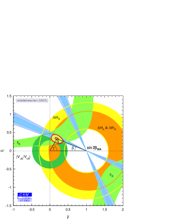
also known as unitarity triangle. Latest experimental results give the following values for the parameter in the Wolfenstein parametrization:

$$\lambda = 0.2279\pm 0.0032$$ (2.28)

$$A = 0.768-0.824$$ (2.29)

$$\overline{\rho} = 0.118-0.273$$ (2.30)

$$\overline{\eta} = 0.305-0.393.$$ (2.31)

These values are consistent with the unitarity of the CKM matrix, as shown in the figure (2.1) [11]. Once again the Standard Model seems to withstand experimental tests.

2.3 Quantum Chromodynamics

Hadrons are particles interacting through strong interactions: since the 30s-40s, from Yukawa’s theory of strong forces on, they were studied to find a coherent theory of this kind of forces. Theoretical attempts have clashed with the large coupling constant associated to these interactions which would have precluded any perturbative expansion.
This difficulty was overcome in the 70s with the discovery of Quantum Chromodynamics (QCD). QCD is a non abelian gauge theory introducing a new quantum number, called color, which exists in three different forms: red, blue and green. The fundamental fields of the theory are the quarks , which carry the charge of color and interact with each other by exchanging the carriers of the strong force, called gluons.
Experiments suggest that colored particles cannot be observed as free states in nature and to explain this evidence an additional property, the confinement, has been postulated.
In this picture, colored particles are confined into hadrons and they are combined in such a way that the color is screened outside the hadron and does not show up.
A description of the confinement is not yet possible: in particular we cannot solve completely the theory, starting from the lagrangian of QCD, written in term of fundamental fields (quarks and gluons), to explain the spectrum of the bound states observed in nature, i.e. the hadrons.
In spite of the lacking of this complete solution, QCD can explain in great detail strong interactions in high energy experiments.
Although strong interactions involve a large coupling constant at low energies, the application of renormalization group equations shows that, at higher energies, the coupling constant becomes rather small and a perturbative approach is viable.
This occurs because

$$\alpha_{S}(Q^{2})\ll 1\ \ \rm for\ \ Q^{2}\gg\Lambda^{2}_{QCD}$$ (2.32)

where $\Lambda_{QCD}$ is the typical scale of strong interactions, $\Lambda_{QCD}\sim 200\ \rm MeV$ and $Q$ is the hard scale of the process, that is the highest energy scale where the process takes place.
At energies comparable with $\Lambda_{QCD}$ the coupling constant blows up and any perturbative approach is barred. This behaviour can qualitatively explain the origin of confinement: when quarks separate (large distances correspond to small exchanged momenta), the interaction between them becomes stronger and stronger, in such a way that they can never be further than a distance corresponding to the typical scale of QCD.
During the times different techniques were developed in field theory to deal with the non perturbative region of strong interactions, such as for example QCD sum rules and lattice QCD.
On the contrary the perturbative part has been widely studied and tested in the last twenty five years and perturbative QCD has become a precision tool to deal with strong interactions in high energy physics.
In the next sections some of the most important features of QCD will be briefly recalled, above all those properties which are needed further down.

2.4 The Parton Model

In the 60s experiments performed at the Stanford Linear Accelerator Center (SLAC), showing the so called Bjorken scaling [12], and spectroscopical observations suggest that mesons (bosonic hadrons) and baryons (fermionic hadrons) are composed by building blocks which, at high energies, interact with external currents as free particles.
These constituents were called partons, the name introduced by Feynman, or quarks, as they were called by Gell-Mann [13]. On theoretical basis also Zweig [14] introduced a similar entity.
Experiments at SLAC, pointing out the partonic behaviour at high energies, concerned Deep Inelastic Scattering, that is the scattering of an electron over a proton with a large exchanged momentum (that is a momentum much larger than the proton mass). In terms of the Bjorken variable

$$x=-\frac{q^{2}}{2P\cdot q}$$ (2.33)

where $q^{\mu}$ is the exchanged momentum and $P^{\mu}$ the proton momentum (usually taken in its rest frame, where $P^{\mu}=(M,0)$). In first approximation the structure functions $f_{a}(x)$, representing the probability to find a parton of type $a$ in the hadron with a value $x$ of the Bjorken variable, measured in the process do not depend on $x$ (Bjorken scaling). As it was noticed, this is the typical situation occurring in point-like elastic scatterings: this behaviour can be explained assuming that the electron is scattered by a point-like constituent inside the proton, suggesting that at high energies hadrons can be thought as composed by partons, which behave as free particles.
At the beginning of the 60s, to explain hadron spectroscopy, three types of quarks were introduced: up, down and strange. In the following years other three quarks were discovered: the charm quark in 1974, bottom or beauty in 1977 and , finally, the top quark in 1994.
The first three quarks have masses negligible at high energies and for this reason they are usually referred as light quarks. The three quarks discovered more recently are referred as heavy quark, because their mass is in general relevant.

$$m_{c} \simeq 1.5{\rm GeV},$$

$$m_{b} \simeq 5{\rm GeV},$$

$$m_{t} \simeq 175{\rm GeV}.$$ (2.34)

This is true for the top and, in many processes (and in particular the ones we are interested in), for the beauty. The mass of the charm quark is relevant in many processes, but the application of perturbative QCD at charm mass energies is doubtful, since the coupling constant is quite large $\alpha_{S}(m_{c})=g^{2}/4\pi\simeq 0.35$.
The parton model was introduced by Feynman and Bjorken for light quarks, assuming that each parton in the hadron carries a fraction of the total quadrimomentum of the hadron itself. Defining $f_{a}(z)$ the probability to find a parton of type $a$, carrying a momentum fraction $z$, the cross section $d\sigma$ for the Deep Inelastic Scattering can be written as

$$d\sigma=\sum_{a}\int_{0}^{1}dz\ f_{a}(z)\ d\hat{\sigma}_{a}(z)$$ (2.35)

where $d\hat{\sigma}$ is the partonic cross section, that is the cross section for the scattering of an electron over a quark $a$.
At first the parton model was a naïve picture which did not take into account strong corrections: an improved parton model can be consistently introduced considering QCD corrections, which explain for example Bjorken scaling violations.
Eq.(2.35) shows a paradigmatic situation in QCD, the interplay between non perturbative and perturbative terms, which contribute together to the result, but can be obtained in different ways: $d\hat{\sigma}_{a}(z)$ being a point-like object can be in principle computed in perturbation theory, while the parton distribution functions (pdf), being log distance objects, cannot be calculated and have to be extracted by experimental data. However the theory allows to calculate perturbatively the evolution of the pdf’s as a function of the scale.

2.5 The Lagrangian of Quantum Chromodynamics

QCD is a non abelian gauge theory, whose group of symmetry is $SU(3)_{c}$. The index $c$ indicates that the quantum number is the color.
The Lagrangian of QCD is obtained according to Yang-Mills theories, by requiring a local invariance under the group $SU(3)_{c}$. The construction of the Lagrangian involves the definition of a covariant derivative

$$(D^{\mu})_{ab}=\partial^{\mu}\delta_{ab}+ig_{s}\ (t^{c}A^{\mu c})_{ab}$$ (2.36)

where $A^{\mu}(x)$ are gluons, the gauge fields of the theory, and $t^{a}$ are matrices of the fundamental representation of $SU(3)$, having the properties

$$\left[t^{A},t^{B}\right]=if^{ABC}t^{C}$$ (2.37)

being $f^{ABC}$ the structure constants of $SU(3)$.
The most common choice is provided by the eight Gell-Mann matrices, hermitean and traceless, normalized as

$${\rm Tr}\ t^{A}t^{B}=\frac{1}{2}\delta^{AB}$$ (2.38)

Important relations satisfied by the colour matrices are

$$\sum_{A}t^{A}_{ab}t^{A}_{bc}=C_{F}\delta_{ac}\ \ \ {\rm{with}}\ \ \ C_{F}=\frac{4}{3}.$$ (2.39)

For the adjoint representation it holds

$${\rm{Tr}}\ \mathit{T}^{A}T^{B}=C_{A}\delta_{AB}\ \ \ {\rm{with}}\ \ \ C_{A}=3$$ (2.40)

The lagrangian density describing the interaction between fermionic fields $q(x)$ (quark) and gauge bosons (gluons), locally invariant under $SU(3)$ turns out to be:

$$\mathcal{L}_{QCD}=-\frac{1}{4}F^{a}_{\mu\nu}F^{a\mu\nu}+\sum_{flavours}\overline{q}_{a}(iD\!\!\!\!/-m)_{ab}q_{b}$$ (2.41)

where $F^{a}_{\mu\nu}$ is the strength tensor defined as

$$F^{a}_{\mu\nu}=\left[\partial_{\mu}A^{a}_{\nu}-\partial_{\nu}A^{a}_{\mu}-g_{s}f^{abc}A^{b}_{\mu}A^{c}_{\nu}\right].$$ (2.42)

The indices $a,b,c$ run over the eight degrees of freedom of the gluon field.
Feynman rules deriving from this lagrangian are contained in appendix (A).

2.6 Evolution of the Coupling Constant and Asymptotic Freedom

Let us consider an observable $\mathcal{O}(Q^{2})$, where $Q$ is an energy scale much larger than every other energy parameter involved in the process, for example the masses of the quarks, $Q^{2}\gg m^{2}_{i}$. In general a prediction about the value of this observable can be performed in perturbation theory, that is as an expansion in the coupling constant

$$\alpha_{s}=\frac{g^{2}_{s}}{4\pi},$$ (2.43)

provided that $\alpha_{S}$ is small enough to justify this approach. Obviously let us consider an observable where only strong corrections need to be calculated.
In order to remove ultraviolet divergences, arising to every order of the perturbative expansion, the theory of renormalization has to be applied to the observable $\mathcal{O}(Q^{2})$, by introducing a substraction point $\mu$. Now, having introduced a second energy scale, the observable $\mathcal{O}$ will depend on the ratio $Q^{2}/\mu^{2}$.
However the renormalization scale $\mu$ is arbitrary and, according to the theory of renormalization, the observable $\mathcal{O}(Q^{2}/\mu^{2})$ has to satisfy the Callan-Symanzik equation (renormalization group equation):

$$\mu^{2}\frac{d}{d\mu^{2}}\mathcal{O}(\frac{Q^{2}}{\mu^{2}},\alpha_{S})\equiv\left[\mu^{2}\frac{\partial}{\partial\mu^{2}}+\mu^{2}\frac{\partial\alpha_{S}}{\partial\mu^{2}}\frac{\partial}{\partial\alpha_{S}}\right]\mathcal{O}(\frac{Q^{2}}{\mu^{2}},\alpha_{S})=0.$$ (2.44)

Defining the $\beta$ function as

$$\beta(\alpha_{S})=\mu^{2}\frac{\partial\alpha_{S}}{\partial\mu^{2}}$$ (2.45)

and defining $t=\log(Q^{2}/\mu^{2})$, the equation (2.44) can be written as

$$\left[-\frac{\partial}{\partial t}+\beta(\alpha_{S})\frac{\partial}{\partial\alpha_{S}}\right]\mathcal{O}(e^{t},\alpha_{S})=0.$$ (2.46)

An implicit solution of this equation is given by

$$\mathcal{O}(\mu^{2}=Q^{2},\alpha_{S}(Q^{2}))=\mathcal{O}(1,\alpha_{S}(Q^{2})),$$ (2.47)

where the new function $\alpha_{S}(Q^{2})$, the running coupling constant , is defined according to the property

$$\int_{\alpha_{S}(\mu^{2})}^{\alpha_{S}(Q^{2})}\ \frac{d\alpha}{\beta(\alpha)}=\log\left(\frac{Q^{2}}{\mu^{2}}\right).$$ (2.48)

Let us remark that in this way the whole dependence on the scale is absorbed in the running coupling constant.
The function $\beta(\alpha_{S})$ admits a perturbative expansion in the form

$$\beta(\alpha_{S})=-\beta_{0}\alpha_{S}^{2}-\beta_{1}\alpha_{S}^{3}-\beta_{2}\alpha_{S}^{4}-\dots$$ (2.49)

and substituting (2.49) into (2.45), the running of the coupling can be calculated in perturbation theory.
The coefficients $\beta_{n}$ can be calculated from higher order corrections to the bare vertices of the theory: at present they are known up to fourth order. For our purposes only $\beta_{0}$ and $\beta_{1}$ will be relevant:

$$\beta_{0} = \frac{33-2n_{f}}{12\pi},$$

$$\beta_{1} = \frac{153-19n_{f}}{12\pi^{2}},$$ (2.50)

where $n_{f}$ is the number of the active flavours at the energies where the process takes place.
The leading order solution of the equation (2.45) reads

$$\alpha_{S}(Q^{2})=\frac{\alpha_{S}(Q_{0}^{2})}{1+4\pi\beta_{0}\log(Q^{2}/Q_{0}^{2})}.$$ (2.51)

In this way we can extract the value of the coupling constant at a scale $Q$, known its value at $Q_{0}$. The most common choice is to consider as a reference $\alpha_{S}(M^{2}_{Z^{0}})$ which is a parameter of the Standard Model known with very high precision.

$$\alpha_{S}(M^{2}_{Z^{0}})=0.11720\pm 0.00017$$ (2.52)

Another choice to express the solution of (2.45) is possible: one can introduce a parameter $\Lambda_{QCD}$ in such a way that (2.51) takes the form

$$\alpha_{S}(Q^{2})=\frac{4\pi}{\beta_{0}\log\left(Q^{2}/\Lambda^{2}_{QCD}\right)}.$$ (2.53)

In this way the running coupling constant is expressed in terms of one single parameter and it is evident that it blows up when the energy scale is set equal to $\Lambda_{QCD}$.
The exact value of $\Lambda_{QCD}$ strongly depends on its precise definition, but it can be considered of the order of $\Lambda_{QCD}\sim 200\ \rm{MeV}$. Roughly speaking, for energies of the order of a few hundred MeV, the perturbative approach for strong interactions is not reliable because $\alpha_{S}$ becomes too large. Let us notice that this is the typical scale of masses of light hadrons and this suggests that the large growth of the running coupling at low energies is an ingredient necessary to explain phenomena such as the confinement of the quarks inside the hadrons.
On the contrary when the scale of the process becomes very large, the running coupling constant vanishes:

$$\alpha_{S}(Q^{2})\rightarrow 0\ \ \ {\rm for}\ \ \ Q^{2}\rightarrow\infty.$$ (2.54)

This property is known as asymptotic freedom and was discovered by Wilczek, Politzer and Gross in 1974 [15]. Asymptotic freedom is a fundamental property of QCD:

• it justifies the perturbative approach for energies much larger than $\Lambda_{QCD}$: since $\alpha_{S}$ becomes small enough, one can expand any observable in powers of this parameter;

• it explains why the parton model is a successful picture of the structure of an hadron: for large $Q^{2}$ the partons in the hadrons behave as non interacting particles in first approximation, because the coupling constant is small. Through radiative corrections one can calculate violations to this behaviour.

Let us observe that the existence of asymptotic freedom is related to the sign of $\beta_{0}$: as long as the number of flavour is $n_{f}<33/2$ (as it happens in nature), the first coefficient $\beta_{0}$ is positive, that is the first term in the expansion (2.49) is negative. A step-by-step solution of equation (2.44) would show that $\alpha_{S}(Q^{2})$ becomes smaller and smaller as the energy becomes larger because of the sign of $\beta_{0}$.
This behaviour is opposite with respect to QED, where $\beta_{0}=-\frac{1}{3\pi}$ (according to the conventions of eq. (2.49)) [16].
The physical origin of this difference arises from the non abelian nature of QCD: being a non abelian theory gauge bosons carry the quantum number of the symmetry group, the color, contrarily to what follows in QED, where photons do not carry any electric charge. This implies that gluons can interact with each other, as shown by Feynman rules in appendix A . In QED the coupling constant decreases at large distances (small energies) and this effect is naïvely explained as a consequence of vacuum polarization by electron-positron pairs, which screen the electric charge.
In QCD this effect related to quark interactions is overwhelmed by an anti-screen effect due to gluons self-interactions, which causes a growth of the coupling constant at large distances.
Just to conclude this section let us notice that in next applications, instead of (2.53), we will use the following expression for $\alpha_{S}(Q^{2})$:

$$\alpha_{S}(Q^{2})=\frac{4\pi}{\beta_{0}\log\left(Q^{2}/\Lambda^{2}_{QCD}\right)}\left[1-\frac{\beta_{1}}{\beta_{0}}\frac{\log\log\left(Q^{2}/\Lambda^{2}_{QCD}\right)}{\log\left(Q^{2}/\Lambda^{2}_{QCD}\right)}\right],$$ (2.55)

which represents the running coupling constant calculated with next-to-leading accuracy.

2.7 Infrared Divergencies

Infrared divergencies and their cancellation, which is a crucial test of the consistency of a massless theory as QCD and QED, will be one of the main topics of this thesis.
Let us consider a generic process involving at least a quark as an external leg and assume that the quark mass can be neglected with respect to the other relevant energy scales.
Strong corrections to this process involve gluon bremsstrahlung: for example, for one real gluon emission, a straightforward calculation shows that the emission rate turns out to be proportional to the term

$$\Gamma\propto\int_{0}^{1}\ \frac{d\omega}{\omega}\ \int_{0}^{1}\ \frac{d\theta}{(1-\cos\theta)},$$ (2.56)

where $\omega$ is an adimensional and unitary variable, defined as

$$\omega=\frac{E_{gluon}}{E^{MAX}_{gluon}}$$ (2.57)

and $\theta$ is the angle between the gluon and the quark.
The expression in (2.56) is manifestly divergent and, in particular, it shows two types of singularities:

• when the gluon momentum vanishes

  $$\omega\rightarrow 0$$ (2.58)

  the so called soft singularity arises. It originates from the massless nature of the gluon and can be regularized by giving to it a fictious mass $\lambda$;

• when the angle of emission vanishes

  $$\theta\rightarrow 0$$ (2.59)

  the singularity is called collinear. It can be regularized by giving a mass $m$ to the quark.

Soft and collinear singularities will be referred with the comprehensive term of infrared divergencies (or singularities).
In general infrared singularities arise in theories when a massless field is present (soft divergence), the gluon in QCD, or when it couples to another massless field (collinear divergence), for example to a quark [17].
With the regularization indicated above, (2.56) reads:

$$\Gamma\propto\int_{\lambda}^{1}\ \frac{d\omega}{\omega}\ \int_{m^{2}}^{1}\ \frac{d\theta}{(1-\cos\theta)}.$$ (2.60)

After two simple integrations one gets that the singularities are parametrized in terms such as $\log\lambda$ and $\log m$.
This regularization is not the one we will use in explicit calculation: we will use dimensional regularization [18], which is more elegant and theoretically useful, even if it hides the origin of the singularities discussed above. In practice one calculates integrals in $N=4+\epsilon$ dimensions, instead of 4 dimensions: in this number of dimensions infrared divergent integrals becomes regular and singularities are parametrized as poles in the regulator $\epsilon$. Once divergencies are removed in such a way, one can consider the limit $\epsilon\rightarrow 0$, coming back to a physical number of dimensions.
In this regularization scheme the equation (2.56) takes the form

$$\Gamma\propto\int_{0}^{1}\ \frac{d\omega}{\omega^{1-\epsilon}}\ \int_{0}^{1}\ \frac{d\theta}{(1-\cos\theta)^{1-\epsilon/2}}=\frac{2}{\epsilon^{2}}.$$ (2.61)

More details about this topic will be discussed in chapter 7 where explicit calculation will be shown.

2.8 Cancellation of Infrared Divergencies

Obviously meaningful physical results cannot be affected by singularities: somehow infrared divergencies have to be cancelled.
At first let us consider the case of inclusive quantities, such as for example the total rate of a scattering or the total width of a decay.
The non abelian nature of QCD complicates the question: let us recall at first the solution for QED, which is an abelian theory.
In QED it is known from a very long time that infrared divergencies arise in photon brehmsstrahlung processes and in radiative corrections in general. Their cancellation is assured by Bloch-Nordsieck theorem [19]: it states that infrared singularities cancel if we sum over all the degenerate final states. In practice, order by order in perturbation theory, one has to sum all the real and virtual diagrams describing the same process: for example, for one photon emission one has to take into account photon brehmasstrahlung and virtual one loop diagrams with no photon emission.
From a physical point of view, the explanation of this theorem is rather intuitive: for soft emission , for example, one should consider that every real detector has a finite resolution and cannot distinguish between an electron and an electron plus a soft photon. In practice the bare state of electron does not exist: a physical electron is always surrounded by a cloud of soft photons.
Analogous considerations can be made for collinear singularities: every detector cannot resolve particles in a arbitrarily small angular cone, so that a summation over the state of electron and electron plus a cloud of collinear photon is required.
However in non abelian theories the Bloch-Nordsieck theorem is in general violated, as a direct consequence of the non abelian nature of the theory [21, 24].
The cancellation of infrared singularities in non abelian theories is assured, on the basis of general arguments, by the Kinoshita-Lee-Nauenberg theorem, which provides a generalization of Bloch-Nordsieck assertions. The main results of this important theorem are recalled in the next section.

2.8.1 Kinoshita-Lee-Nauenberg Theorem

According to the Kinoshita-Lee-Nauenberg theorem [22, 23] the cancellation is attained when a summation over final degenerate states (like in Bloch-Nordsieck theorem) and initial degenerate states (due to the non abelian nature of the theory) is performed.

Figure 2.2: Example of two diagrams having the same final states.

In particular, in Kinoshita’s work [22], the relation between the Feynman diagrams involved in the process and the cancellation of mass (another usual name for collinear divergencies) and soft singularities is widely discussed.
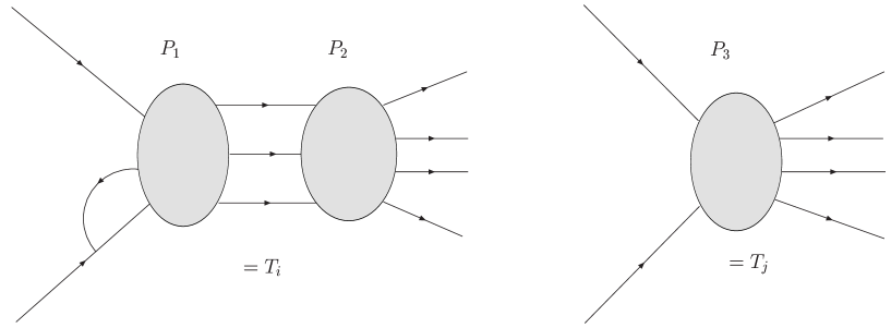
Let us recall the main results of [22]: let us consider a process at a given order of perturbation theory; let us call $T_{i}$ the corresponding Feynman amplitude (see Fig.(2.2)), the total transition probability is proportional to $\sum_{ij}T^{\dagger}_{i}T_{j}$, where the sum over indices is performed considering diagrams with the same final states. $T^{\dagger}_{i}$ is represented by a diagram obtained by $T_{i}$ by reversing time, that is by the exchange of initial and final states.
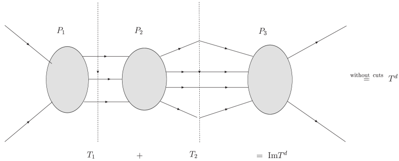
In this way $T^{\dagger}_{i}T_{j}$ may be represented joining the final states of $T_{j}$ and the initial states of $T^{\dagger}_{i}$ (that is the final states of $T_{i}$): in order to distinguish it from a Feynman diagram let us draw a line intersecting the final states of $T_{i}$ and $T_{j}$.
Let us call $T^{d}$ the Feynman diagram obtained removing the cutting line and consider all the $T^{\dagger}_{i}T_{j}$ which reduces to $T^{d}$ when the line is removed: by the optical theorem $\sum_{ij}T^{\dagger}_{i}T_{j}$, with the sum over the diagrams which reduce to $T^{d}$ when the cutting line is removed, is the absorbitive part $A^{d}$ of $T^{d}$ and it’s called cut diagram (see Fig.(2.3)).

Figure 2.3: Example of cut diagrams: $T_{1}$ and $T_{2}$ are two different cuts of the same diagram $T^{d}$.

The total transition probability is the sum of cut diagrams involved in the process.
Let us now connect the initial states of $T^{d}$ with its final states (remember that they carry the same momentum), that is the initial states of $T_{i}$ and $T_{j}$ and let us represent this junction with a second cutting line.
Removing the cutting lines we obtain a vacuum-to-vacuum transition $T^{v}$: let us consider the set $\Delta$ of diagrams $\Delta_{i}$ which reduce to $T^{v}$ by removing the cutting lines (see Fig.(2.4)).
$\Delta$ is called a double cut diagram and the total transition probability is a sum of $\Delta$s.

Figure 2.4: Example of double cut diagram: the amplitudes $\Delta_{1}$,$\Delta_{2}$ and $\Delta_{3}$ belong to the same set $\Delta$.

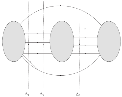
Kinoshita’s paper [22] shows that not only the total transition probability is free from infrared divergences but also every $\Delta$ doesn’t show neither soft singularities nor collinear (or mass) ones.

2.8.2 Cancellation of Infrared Singularities in QCD

In principle, in QCD the summation over initial states would be required, according to what stated above.
In many processes however Bloch-Nordsieck theorem can be applied, provided that a summation over initial and final color is performed; actually this is first of all a phenomenological requirement: because of confinement colored particles cannot be observed, so that a summation over all the possible color is natural, since only this superposition is observable.
However some counterexamples have been found, where the only summation over colors is not sufficient: for examples in [24] has been found that in Drell-Yan

$$q\overline{q}\rightarrow\gamma X,$$ (2.62)

where $X$ is every hadronic state, subleading soft divergencies arise at two loops and they are not cancelled by soft gluon emissions. If the degeneracy of the initial quark with the state of a quark plus a soft gluon is taken into account, this divergence is cancelled. This is nothing but an application of the Kinoshita-Lee-Nauenberg theorem.
Let us underline that this is not necessary for our purposes and in our explicit calculation the simple summation over colors and final states will be enough.

2.8.3 An Example: Incomplete Cancellation of Infrared Logarithms in the Electroweak Sector

In the last few years, some authors [20, 21] showed that Bloch-Nordsieck violations can be observed also in the electroweak sector of the Standard Model. This happens since the Glashow-Weinberg-Salam model is based on a non abelian gauge theory. It assumes particular characteristics because of some peculiarity of the theory.
Apart the photon, whose behaviour in QED is discussed above and it is not interesting here, the gauge bosons of electroweak interactions, $W^{\pm}$ and $Z^{0}$, are massive. The mass provides a natural cut off: in this case infrared singularities are screened, but residual large logarithms, such as

$$\frac{\alpha_{W}}{\pi}\log^{2}\left(\frac{M^{2}_{W}}{Q^{2}}\right),$$ (2.63)

arise as in (2.60), though here the cut off mass is physical and not fictious.
In [20, 21] authors noticed that these logarithmic terms do not cancel even in inclusive quantities: in QED and QCD large infrared logarithms appear in semi-inclusive distributions (they will be introduced in section (2.10)), but cancel in inclusive quantities, such as total rates.
The appearance of residual logarithms in the Electroweak Model is a violation of the Bloch-Nordsieck theorem, due to the non abelian nature of the theory: in this case a summation over initial weak charges is not required, contrarily to what performed in QCD with initial colors, because particles carrying weak isospin can exist as asymptotic states, for example as electrons or neutrinos.
This implies that in processes such as

$$e^{+}e^{-}\rightarrow\ \rm everything$$ (2.64)

terms like (2.63) remain.
A cancellation of these terms would be achieved by summing the rate $\sigma(e^{+}e^{-}\rightarrow\ \rm everything)$ to the rate $\sigma(\overline{\nu}_{e}+e^{-}\rightarrow\ \rm everything)$: this corresponds to a summation over initial state weak charges and, according to KLN theorem, provides the cancellation of logarithms. Obviously there is not a compelling physical reason to do that.
The presence of terms (2.63) does not spoil the theory: after all they are finite and not singular, even if they are a sort of shadow of the infrared singularity.
However, at asymptotic energies, these terms can become large and enhance electroweak corrections, even if $\alpha_{W}$ is quite small, making electroweak corrections comparable to strong ones. If this effect does exist, it will be surely detectable at future Linear Colliders.

2.9 Evolution Equations

Evolutions equations are an important property of QCD dynamics [25, 26].
Let us consider multiple branching of partons from another one, for example multiple emissions of gluons from a quark or splitting of a gluon into a quark-antiquark pair and so on.

Figure 2.5: Evolution of a light quark outgoing from an hard process at the energy $Q^{2}$. Through multiple gluon emissions it evolves from the virtuality $t_{n}$ to the virtuality $t_{0}$.

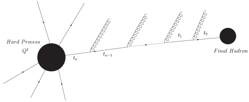
As shown in picture (2.5), the parent parton, participating to an hard process at a scale $Q^{2}$, evolves emitting other partons (gluons or quark) and increasing its virtual mass-squared, as it approaches the hard process. In order to be plain we can consider an outgoing quark from the hard process, having virtual mass-squared $-t_{n}$, carrying a momentum fraction $x_{n}$, which evolves to less virtual masses and momentum fraction, by emitting multiple gluons at small angles.
The total rate of the hard process will depend on the momentum fraction distribution of the partons $f_{i}(x,Q^{2})$ inside the hadron, as seen by an external probe (for example the virtual photon in the deep inelastic scattering).
GLAPD (Gribov-Lipatov-Altarelli-Parisi-Dokshitzer) [25, 26] evolution equations describe the evolution of the distribution $f_{i}(x,Q^{2})$ changing the scale of the hard process: they are a set of coupled integro-differential equations

$$t\frac{\partial}{\partial t}f_{i}(x,t)=\sum_{j}\int_{x}^{1}\frac{dz}{z}\frac{\alpha_{S}}{2\pi}P_{ij}(z)f_{j}(x/z,t).$$ (2.65)

The index $j$ runs over the different types of partons, that is quark ($q$), antiquark ($\overline{q}$) and gluon ($g$).
The kernels in the equations, $P_{ij}(z)$ are called the parton splitting functions, taking into account different types of branching: pair production from a gluon $P_{qg}$, gluon emission from a quark $P_{qq}$ and gluon splitting into gluons $P_{gg}$.
The charge conjugation invariance implies

$$P_{q_{i}q_{j}} = P_{\overline{q}_{i}\overline{q}_{j}}$$

$$P_{q_{i}\overline{q}_{j}} = P_{\overline{q}_{i}q_{j}}$$

$$P_{\overline{q}_{i}g} = P_{q_{i}g}\equiv P_{qg}$$

$$P_{g\overline{q}_{i}} = P_{gq_{i}}\equiv P_{gq}$$ (2.66)

They can expanded in perturbation theory as

$$P_{ij}(z)=\frac{\alpha_{S}}{2\pi}P^{(0)}_{ij}(z)+\left(\frac{\alpha_{S}}{2\pi}\right)^{2}P^{(1)}_{ij}(z)+\dots$$ (2.67)

At the lowest order they take the look [25]

$$P^{(0)}_{qq}(z) = C_{F}\left[\frac{1+z^{2}}{(1-z)_{+}}+\frac{3}{2}\delta(1-z)\right],$$ (2.68)

$$P^{(0)}_{qg}(z) = n_{f}\frac{z^{2}+(1-z)^{2}}{2},$$ (2.69)

$$P^{(0)}_{gq}(z) = C_{F}\left[\frac{1+(1-z)^{2}}{z}\right],$$ (2.70)

$$P^{(0)}_{gg}(z) = 2C_{A}\left[\frac{z}{(1-z)_{+}}+\frac{1-z}{z}+z(1-z)\right]+\frac{11C_{A}-2n_{f}}{6}\delta(1-z).$$ (2.71)

The next-to-leading order kernels, $P^{(1)}_{ij}$ have been calculated in [27].
The symbol ”+” denotes plus distributions, defined through the relation

$$\int_{0}^{1}dz\ \frac{g(z)}{(1-z)_{+}}\equiv\int dz\ \frac{g(z)-g(1)}{1-z}.$$ (2.72)

Let us notice that the plus distribution removes the infrared singularities for $z\rightarrow 1$: in fact the ”+” distribution reproduces the summation between real and virtual diagrams, which assures the cancellation of singularities. Let us finally remark that the singularity for $z\rightarrow 0$ is outside the domain of integration.
The parton splitting function can be naïvely interpreted as the probability to emit a parton with momentum fraction $z$ by the parent parton: the interpretation as probability implies that

$$\int_{0}^{1}dxP_{qq}^{(0)}(x)=0,$$

$$\int_{0}^{1}dx\ x\left[P_{qq}^{(0)}(x)+P_{gq}^{(0)}(x)\right]=0,$$

$$\int_{0}^{1}dx\ x\left[2n_{f}P_{qg}^{(0)}(x)+P_{gg}^{(0)}(x)\right]=0.$$ (2.73)

Actually the interpretation as probability is formally incorrect, because it does not handle carefully the infrared singularity for $z\rightarrow 1$.
A more correct interpretation can be introduced, by defining the Sudakov form factor

$$\Delta_{i}(Q,Q_{0})\equiv\exp{\left[-\sum_{j}\int_{Q_{0}}^{Q}\frac{dQ^{\prime}}{Q}\int dz\frac{\alpha_{S}}{2\pi}P_{ji}(z)\right]}$$ (2.74)

which turns out to be the probability to evolve from the scale $Q_{0}$ to $Q$ without any branching [28].
A final observation is necessary for our purposes: as long as a single logarithmic accuracy is required, instead of the bare coupling one should consider the running coupling, evaluated at the transverse momentum squared, as suggested in [29],

$$\alpha_{S}\rightarrow\alpha_{S}\left[z(1-z)Q\right].$$ (2.75)

The effect of this redefinition of the scale where to evaluate the coupling constant, is necessary at next-to-leading order: in fact, expanding the running coupling one has

$$\alpha_{S}(z(1-z)Q)=\alpha_{S}(Q)+\beta_{0}\log\left[z(1-z)\right]\frac{\alpha_{S}^{2}(Q)}{4\pi}+O(\alpha_{S}^{3}).$$ (2.76)

At two loops, the logarithmic term, combined with the soft singularity $1/(1-z)$, gives next-to-leading terms: since we have performed calculation with next-to-leading accuracy, these terms due to the running of the coupling cannot be neglected.

2.10 Semi-inclusive Observables and Infrared Logarithms

Another approach to study the properties of strong interactions is to define quantities which are not fully inclusive, but select particular region of the phase space.
Among these distributions are the so called shape variables , which permits to characterized the shape of the final hadronic jet: an example is the thrust , defined as [30]

$$T=\ {\rm max}_{n}\ \frac{\sum_{i}|\vec{p}_{i}\cdot\vec{n}|}{\sum_{i}|\vec{p}_{i}|},$$ (2.77)

where $\vec{n}$ is an arbitrary an unitary vector.
In practice one wants to define a variable $X$, which in our calculation will be the transverse momentum, and calculate the differential distribution

$$d(X)=\frac{1}{\Gamma_{0}}\ \frac{d\Gamma}{dX},$$ (2.78)

or the partially (cumulative) integrated distribution

$$D(X)=\frac{1}{\Gamma_{0}}\ \int_{X_{0}}^{X}\ dX^{\prime}\frac{d\Gamma}{dX^{\prime}},$$ (2.79)

where $X=X_{0}$ is the elastic point, that is the Born (lowest order) value of the observable. Let us consider the case where

$$\frac{1}{\Gamma_{0}}\ \frac{d\Gamma}{dX}=\delta(X-X_{0})$$ (2.80)

and

$$\frac{1}{\Gamma_{0}}\ \int_{X_{0}}^{X}\ dX^{\prime}\frac{d\Gamma}{dX^{\prime}}=1.$$ (2.81)

Radiative corrections spread the spectrum in general and introduced theoretical problems to face: in order to be calculable in perturbation theory, the considered quantity has to be infrared safe. Higher order corrections show infrared singularities for real and virtual emission separately: in infrared safe quantities these singularities cancel in the sum of real and virtual diagrams as stated in the sections above.
Another way to state this property is requiring that the observable is insensitive to the emission of soft or collinear gluons, that is it is invariant under the branching

$$\vec{p_{i}}\rightarrow\vec{p_{j}}+\vec{p_{k}}$$ (2.82)

where the final momenta are collinear or one of them is very small.
At the order $O(\alpha_{S})$ the calculation can be performed inserting in the phase space a kinematical constraint, describing the distribution we want to calculate, in terms of the variable of the system:

$$\frac{1}{\Gamma_{0}}\ \frac{d\Gamma}{dX}=\frac{1}{\Gamma_{0}}\int_{\Omega}\ \frac{d\Gamma}{d\Omega}\ \delta(X-o(\Omega))\ d\Omega,$$ (2.83)

where $\Omega$ represents generically the set of variables which parametrize the phase space. $o(\Omega)$ is a function of the kinematical variables of the system and, in order to have an infrared safe distribution $o(\Omega)$ has to vanish for soft emissions and for collinear emissions:

$$o(\Omega)\rightarrow 0\left\{\begin{array}[]{l@{\quad}l}{\rm for}\ E_{gluon}\rightarrow 0\\ {\rm for}\ \theta_{emission}\rightarrow 0\end{array}\right.$$

In this kind of observables the cancellation of infrared singularities occurs, but large logarithms arise in every order of the perturbation theory. In fact the structure of the calculation at a finite order (fixed order), is

$$D(X)=\sum_{m=0}^{2n}\ G_{mn}\log^{m}|X-X_{0}|.$$ (2.84)

These logarithms will be referred as infrared or large logarithms, because they become large when the variable approach the infrared region of the phase space. This occurs for $X\rightarrow X_{0}$, that is near the elastic point of the process and corresponds to the emission of soft or collinear gluons.

2.10.1 General Structure for Single Gluon Emission

As a remarkable example let us consider the rate for one real gluon emission. The contribution to the distribution in a generic variable $u$ is

$$f_{R}(u)=\int_{0}^{1}d\omega\int_{0}^{1}dt\ |{\overline{\cal M}}|^{2}(\omega,t)\ \delta(u-o(\omega,t)),$$ (2.85)

where $|{\overline{\cal M}}|^{2}(\omega,t)$ is the squared amplitude for the emission of one real gluon, integrated over the azimuthal angle and averaged/summed over the helicities and the colors of the initial/final partons. We defined the unitary variables $\omega$ and $t$

$${\omega=}\frac{E_{g}}{E_{g}^{\max}}$$ (2.86)

$${t=}\frac{1-\cos\theta}{2}.$$ (2.87)

The function $o\left(\omega,t\right)$ is the kinematical constraint which specifies the states of the infrared gluon which are included in the distribution and it is rescaled in such a way that

$$0\leq o\left(\omega,t\right)\leq 1.$$ (2.88)

For a collinear-safe observable

$$o\left(\omega,t=0\right)=0$$ (2.89)

while for a soft safe observable we have

$$o\left(\omega=0,t\right)=0.$$ (2.90)

An observable is therefore infrared safe when both conditions above are satisfied, or, in other words when it is unaffected by the emission of a soft and/or collinear gluon. If conditions (2.89) or (2.90) holds we have the cancellation of the two delta functions on the r.h.s. of equation (2.100) for a collinear or soft gluon respectively . As a consequence, the corresponding singularity is screened. The distribution can be therefore computed in perturbation theory in the limit of vanishing parton masses and virtualities.
We know that the amplitude shows a pole in $\omega=0$ (soft singularity), due to the vanishing mass of the gluon, and a pole in $t=0$ (collinear singularity), due to the vanishing mass of the quark.
Therefore we can write [2]

$$|{\overline{\cal M}}|^{2}(\omega,t)=\frac{\,M(\varepsilon,t)}{\omega\,t}=\frac{\alpha_{S}A_{1}}{\omega\,t}+\frac{\alpha_{S}S_{1}(t)}{\omega}+\frac{\alpha_{S}C_{1}(\omega)}{t}+\alpha_{S}F_{1}(\omega,t),$$ (2.91)

where the functions $A_{1},\,S_{1}(t),\,C_{1}(\omega),\,F_{1}(\omega,t)$ are defined as follows:

$$A_{1} \equiv M(0,0),$$ (2.92)

$$S_{1}\left(t\right) \equiv \frac{M(0,t)-M(0,0)}{t},$$ (2.93)

$$C_{1}\left(\omega\right) \equiv \frac{M(\omega,0)-M(0,0)}{\omega},$$ (2.94)

$$F_{1}\left(\omega,t\right) \equiv \frac{M(\omega,t)-M(0,t)-M(\omega,0)+M(0,0)}{\omega\,t}.$$ (2.95)

From their definition it is clear that they are finite in the soft limit

$$\omega\rightarrow 0,$$ (2.96)

as well as in the collinear one

$$t\rightarrow 0.$$ (2.97)

By integrating the amplitude in $\omega$ and $t$ at the border of the phase space, large logarithms arise from the terms which are singular in (2.91):

$$D(X)=1+\frac{\alpha_{S}}{\pi}\left(\tilde{A}_{1}\log^{2}X+B_{1}\log X+\kappa_{1}+r(X)\right).$$ (2.98)

The double logarithm represents the leading term, while the single logarithm is referred as the next-to-leading term, $\kappa_{1}$ is a constant and $r(X)$ is a regular function in the whole phase space, vanishing for $X\rightarrow X_{0}$. $\tilde{A}_{1}$ is strictly related to $A_{1}$, typically $A_{1}$ times some coefficient coming from the variable we are considering. $B_{1}$ is a combination of $C_{1}$ and $S_{1}$.
The leading term is the well known Sudakov double logarithm [32], whose coefficient is $A_{1}$ and have both soft and collinear nature. The next-to-leading term is given by single logarithms of soft or collinear nature. $F_{1}(\omega,t)$ contains the terms which are not singular in the infrared limit.
Let us recall that $f_{R}$ contains infrared divergences which cancel in the sum with virtual diagrams:

$$f(u)=f_{R}(u)+f_{V}(u),$$ (2.99)

giving rise to ”+” distributions, as defined above. $f(u)$ is the physical distribution taking into account real and virtual emissions.
$f(u)$ at the border of the phase space, omitting the finite term $F_{1}(\omega,t)$, which does not product any large logarithm, may be written to $O(\alpha_{S})$ as:

$$f(u)=\delta(1-u)+\alpha_{S}\int_{0}^{1}d\omega\int_{0}^{1}dt\left[{\frac{A_{1}}{\omega t}}+{\frac{S_{1}(t)}{\omega}}+{\frac{C_{1}(\omega)}{t}}\right]\left\{\delta\left[u-o\left(\omega,t\right)\right]-\delta\left[u\right]\right\}.$$ (2.100)

According to the conditions stated the integral of the distribution over the whole kinematical domain is one, i.e. the distribution is normalized:

$$\int_{0}^{1}f(u)\,du=1.$$ (2.101)

This means that the total rate is unchanged with respect to its value by the emission of an infrared gluon.
Obviously the functions $A_{1}$, $S_{1}\left(t\right)$ e $C_{1}\left(\omega\right)$ may be obtained with an explicit evaluation of the Feynman diagrams for the emission of a real gluon. It is however possible to give a general derivation of these functions by using the properties of the amplitudes in the collinear and soft limits, as we will do in the two following paragraphes.

2.10.2 Terms of Collinear Origin

The functions $A_{1}$ and $C_{1}\left(\omega\right)$ may be obtained by considering the perturbative evolution of a light quark in QCD.
Let us define

$$z=1-\omega,$$ (2.102)

$z$ is the energy fraction carried by the light quark, so that

$$o\left(\omega,t\right)=\omega.$$ (2.103)

As we can see from condition (2.89), this observable is not collinear safe: we regulate the collinear divergence with a small quark mass $\mu\neq 0.$ The denominator of the light quark propagator is therefore modified in $\left(p^{2}=\mu^{2}\right)$:

$$\frac{1}{\left(p+k\right)^{2}-\mu^{2}}\cong\frac{1}{Q^{2}}\,\,\frac{1}{\omega\left(t+\mu^{2}/Q^{2}\right)}.$$ (2.104)

where we have defined as usual

$$Q=2p^{0}\ \ ,\ \ \omega={2k^{0}\over Q}$$

The integration over the polar angle is

$$\int_{0}^{1}dt\ {1\over t+{\mu^{2}\over Q^{2}}}=\int_{\mu^{2}\over Q^{2}}^{1}dt^{\prime}{1\over t^{\prime}}$$

This result is the same of the massless case $\left(\mu=0\right)$, with the angular restriction:

$$t>\frac{\mu^{2}}{Q^{2}}.$$ (2.105)

known as dead cone effect.
The fragmentation function may be written as:

$$D(z;Q^{2}) = \delta(1-z)+\alpha_{S}\int_{\mu^{2}/Q^{2}}^{1}\frac{dt}{t}\int_{0}^{1}d\omega\left[{\frac{A_{1}}{\omega}}+C_{1}(\omega)\right]\left[\delta(1-z-\omega)-\delta(1-z)\right]$$ (2.106)

$$= \delta(1-z)+\left[\alpha_{S}A_{1}\left(\frac{1}{1-z}\right)_{+}+\alpha_{S}\,C_{1}(1-z)_{+}\right]\log\frac{Q^{2}}{\mu^{2}}.$$

Let us compare with the fragmentation function to the order $\alpha_{S}$, containing the leading Altarelli-Parisi kernel:

$$D(z;Q^{2}) = \delta(1-z)+{\frac{C_{F}\alpha_{S}}{2\pi}}\left({\frac{1+z^{2}}{1-z}}\right)_{+}\log\frac{Q^{2}}{\mu^{2}}+\ldots$$ (2.107)

$$= \delta(1-z)+\left[{\frac{C_{F}\alpha_{S}}{\pi}}\left({\frac{1}{1-z}}\right)_{+}-\frac{C_{F}\alpha_{S}}{2\pi}\left(1+z\right)_{+}\right]\log\frac{Q^{2}}{\mu^{2}}.$$ (2.108)

The plus-distribution in the infrared regular kernel may be made explicit as:

$$\left(1+z\right)_{+}{=1+z-}\frac{3}{2}{\delta}\left(1-z\right).$$ (2.109)

This decomposition allows the identification

$$A_{1} = \frac{C_{F}}{\pi},$$ (2.110)

$$C_{1}{(1-z)} = {-}\frac{C_{F}}{2\pi}\left(1+z\right)$$ (2.111)

implying that

$$C_{1}{\equiv}\int_{0}^{1}\ dz\ {C}_{1}{(1-z)=}-\frac{3}{4}\frac{C_{F}}{\pi}.$$ (2.112)

This is the usual collinear coefficient appearing at the $\alpha_{S}$ order in processes involving light quarks (DIS, Drell-Yan, …).

2.10.3 Soft Emissions and Eikonal Approximation

In processes involving light quarks only, single logarithms coming from soft emissions do not appear. This means that in these processes soft gluons can be emitted only at small angles, at least in the approximation where only next-to-leading terms are taken into account. It can be proved that, in such an approximation, they are emitted according to an angular ordering, behaviour known as coherence [31]. In processes involving light quarks only, coherence is violated at subleading level.
Instead in processes where also heavy quarks are present coherence is already violated at the next-to-leading level: this means that soft emissions at large angle are possible even at the next-to-leading order.
In general soft emissions can be treated according to the eikonal approximation, by considering the emission of a gluon from the hard on-shell partons which take part to the Born process. In such approximation the amplitude factorizes in the Born amplitude multiplied by the eikonal current:

$${J}^{\mu}\left(k\right)=-g_{S}\sum_{i=1}^{n}\frac{v_{i}^{\mu}}{v_{i}\cdot k}{T}_{i}.$$ (2.113)

$v_{i}$ are the 4-velocities of the hard partons: $v_{i}^{2}=0$ for massless, while $v_{i}^{2}=1$ for massive partons. In the massless case the 4-velocity normalization is given by fixing a non trivial kinematical invariant. $T_{i}$ are linear operators acting in the Fock space for the color of the hard partons:

$${T}_{i}|c_{1}\ldots c_{i}\ldots c_{n}\rangle=\left({T}_{i}\right)_{c_{i}^{\prime}c_{i}}|c_{1}\ldots c_{i}^{\prime}\ldots c_{n}\rangle,$$ (2.114)

where$\left({T}_{i}\right)_{c^{\prime}c}$ is the generator of the parton $i$. This space is the direct product of the single parton spaces:

$$|c_{1}\ldots c_{i}\ldots c_{n}\rangle=|c_{1}\rangle\otimes|c_{2}\rangle\otimes\cdots\otimes|c_{n}\rangle.$$ (2.115)

The color conservation in the QCD interactions may be written in such a scheme as:

$$\sum_{i=1}^{n}{T}_{i}=0.$$ (2.116)

where the sum is over initial/final parton colors.
In general the notation is analogous to the one used for the angular momentum in quantum mechanics.
The matrices $T_{i}$ for different practical cases takes the look

$${\rm quark} \rightarrow (T_{k})_{ij}=t^{a}_{ij}$$

$${\rm antiquark} \rightarrow (T_{k})_{ij}=-t^{a}_{ji}$$

$${\rm gluon} \rightarrow (T_{k})_{ij}=if_{bac},$$ (2.117)

where $f_{abc}$ are structure constant of $SU(3)$ and $t^{a}$ matrices of the fundamental representation.
Let us note that, in the soft case, factorization involves the momenta and the colors of all the hard partons. An important property of the eikonal current is that it is conserved:

$$k_{\mu}{J}^{\mu}\left(k\right)=\sum_{i=1}^{n}{T}_{i}=0.$$ (2.118)

The sum over polarizations may then be substituted with the diagonal part:

$$S_{\mu\nu}\left(k\right)\rightarrow-g_{\mu\nu}.$$ (2.119)

The rate is proportional to the square of the eikonal current

$$-g_{\mu\nu}{J}^{\mu}\left(k\right){J}^{\nu}\left(k\right)=-g^{2}_{S}\sum_{i<j}^{1,n}\frac{2v_{i}\cdot v_{j}}{v_{i}\cdot k\,v_{j}\cdot k}{T}_{i}\cdot{T}_{j}-g^{2}_{S}\sum_{i=1}^{n}\frac{v_{i}^{2}}{\left(v_{i}\cdot k\right)^{2}\,}{T}_{i}^{2}.$$ (2.120)

The second sum in the r.h.s. in the equation (2.120) gets contributions only from massive partons and therefore disappears in the well-know processes as DIS, DY, photon fragmentation, etc., which involve only massless partons. If heavy quarks are involved this term does not disappear, giving rise to logarithms of soft nature.
In the decay of a heavy flavour into a light flavour, as we will consider, the eikonal current may be written as:

$${J}^{\mu}\left(k\right)=\frac{v^{\mu}}{v\cdot k}{T}_{Q}-\frac{n^{\mu}}{n\cdot k}{T}_{q}.$$ (2.121)

We have that $v^{2}=1,\,n^{2}=0.$ We normalize the vector $n$ on the light cone imposing $n\cdot v=1,$ in such a way that $n_{0}=1$ in the rest frame of the heavy flavour.
In the case of our interest, with just two hard colored partons (the heavy and the light quark) and with an hard vertex conserving the color of the quark line, the color conservation reads $T_{Q}=T_{q}.$ Since

$${T}_{Q}^{2}={T}_{q}^{2}={T}_{Q}\cdot{T}_{q}=C_{F}$$ (2.122)

the contribution for a soft gluon emission is:

$$f_{S}\left(u\right) = g^{2}C_{F}\int{\frac{d^{3}l}{(2\pi)^{3}2\omega}}\left[-{\frac{v^{2}}{v\cdot l^{2}}}+{\frac{2n\cdot v}{v\cdot l\,\,\,n\cdot l}}\right]\left\{\delta\left[u-o\left(\omega,t\right)\right]-\delta\left[u\right]\right\}$$ (2.123)

$$= \int_{0}^{1}d\omega\int_{0}^{1}dt\left[\frac{\alpha_{S}C_{F}}{\pi}{\frac{1}{\omega\,t}}-\frac{\alpha_{S}C_{F}}{\pi}{\frac{1}{\omega}}\right]\left\{\delta\left[u-o\left(\omega,t\right)\right]-\delta\left[u\right]\right\},$$

being $v\cdot l=\omega$ and $n\cdot k=2\omega t$. We define the rescaled gluon momentum analogously to (2.86):

$$l^{\mu}\equiv\frac{k^{\mu}}{E_{g}^{\max}}.$$ (2.124)

By comparing with the general expression (2.100),we obtain:

$$A_{1}=\frac{C_{F}}{\pi},\ \ \ \ \ \ \ S_{1}=S_{1}(t)=-\frac{\alpha_{S}C_{F}}{\pi}.$$ (2.125)

As already discussed in the general case, $S_{1}\neq 0$ represent a new contribution with respect to processes involving light quarks only (DIS, Drell-Yan, …).
Let us note that the soft function $S_{1}(t)$ actually does not depend on the polar angle $t$: this fact is related to the choice of the reference frame, since the heavy quark at rest emits soft gluons isotropically; this is a violation of coherence at the next-to-leading order instead of at the NNL one, like in DIS or DY.
By using the soft factorization one can verify the value of $A_{1}$ as obtained before, by using the collinear factorization. This last term appears indeed in both schemes having the soft and the collinear enhancement.

2.11 Resummation of Large Logarithms

As long as $\alpha_{S}\log^{2}|X-X_{0}|\ll 1$ the perturbative approach is reliable, however, when this term becomes comparable to 1 problems arise: logarithmically enhanced terms have comparable sizes to every order of perturbation theory

$$\alpha_{S}^{n}\log^{2n}|X-X_{0}|\sim O(1).$$ (2.126)

Obviously in this situation the perturbative approach is not meaningful: one has to resum at least terms such as (2.126), finding an improved perturbative expansion with a larger domain of applicability.
The theory of resummation of large infrared logarithms has been developed in the last twenty years for QCD processes [33, 36, 38, 39, 35]: the resummation of terms like in (2.126) represents the leading or double logarithmic order. A more refined approximation is preferable to reduce the dependance on the renormalization scale and it consists in the resummation of single logarithmic terms of the form $\alpha^{n}_{S}\log^{n}|X-X_{0}|$. This is the next-to-leading approximation we will require for our calculations. In this way the region of applicability of the improved perturbative expansion is enlarged to $\alpha_{S}\log|X-X_{0}|\lesssim 1$, a much larger region than the one where the fixed order calculation is valid.
The resummation of large logarithms has been widely studied and applied to QCD processes for those observables which exponentiate. They have particular properties: their matrix elements can be factorized by expressing the emission of $n$ infrared (soft or collinear) gluons as the product of $n$ single gluon emissions; moreover the phase space and, in particular, the kinematical constraint have to factorize in the same way.
Under such conditions the perturbative expansion in the infrared region give rise to an exponential series, which resums logarithms with the required accuracy.
The result of the resummation of large logarithms is accomplished by the formula [39]

$$D(X)=K(\alpha_{S})\Sigma(\alpha_{S};X)+R(X;\alpha_{S}).$$ (2.127)

The functions involved in the formula will be the object of the calculations we will perform in Chapters 5 and 7 for the process we are going to consider. Here let us just sum up their meaning and their role:

• $\Sigma(X;\alpha_{S})$ resums large logarithms in exponentiated form. It has a perturbative expansion in the form

  $$\log\Sigma(X;\alpha_{S})=\sum_{n=1}^{\infty}\sum_{m=1}^{n+1}G_{nm}\alpha_{S}^{n}L^{m}=Lg_{1}(\alpha_{S}L)+g_{2}(\alpha_{S}L)+\alpha_{S}g_{3}(\alpha_{S}L)+\dots$$ (2.128)

  where $L=\log X$. The functions $g_{i}$ have the form

  $$g_{i}(z)=\sum_{n=0}^{\infty}g_{i,n}z^{n},$$ (2.129)

  so that the calculation of $g_{1}$ resums leading logarithms, that is terms in the form $\alpha_{S}^{n}L^{n+1}$, $g_{2}$ resums next-to-leading contributions as $\alpha_{S}^{n}L^{n}$, $g_{3}$ next-to-next-to-leading and so on. It is worth noting that, even if the fixed order calculation shows at most two logarithms for each power of $\alpha_{S}$, in the exponentiated formula they are rearranged in such a way that there are only at most $(n+1)$ logarithms for $n$ power of $\alpha_{S}$. $\Sigma(X;\alpha_{S})$ is a universal function, that is does not depend on the specific process, but only on general properties of the theory.

• $K(\alpha_{S})$, the coefficient function, is a short distance process dependent function. It takes into account constant terms, arising to every order of the perturbative expansion, which do not exponentiate. It can be calculated order by order in perturbation theory:

  $$K(\alpha_{S})=1+\kappa_{1}\alpha_{S}+\kappa_{2}\alpha_{S}^{2}+O(\alpha_{S}^{3})$$ (2.130)

• $R(X;\alpha_{S})$, the remainder function, is a process dependent function which takes into account hard contributions without any logarithmic enhancement. It depends on the specific process, the distribution, the kinematics and so on. It can be calculated in perturbation theory:

  $$R(X;\alpha_{S})=r_{1}(X)\alpha_{S}+r_{2}(X)\alpha_{S}^{2}+O(\alpha_{S}^{3})$$ (2.131)

  The property

  $$R(X;\alpha_{S})\rightarrow 0\ {\rm for}\ X\rightarrow X_{0}$$ (2.132)

  holds for the remainder function.

For our calculations we will attain next-to-leading accuracy. In order to achieve this level of approximation several terms need to be calculated:

• the functions $g_{1}$ and $g_{2}$ to resum logarithms with next-to-leading accuracy. In order to reach this goal, running coupling effects should be taken into account, as discussed in section (2.6);

• the value of $\kappa_{1}$ in the coefficient function has to be calculated, because the combination

  $$\alpha_{S}\kappa_{1}\cdot e^{Lg_{1}(\alpha_{S}L)}\sim\kappa_{1}\alpha_{S}^{2}L^{2}$$ (2.133)

  produces next-to-leading contributions.

Moreover, the calculation of the first term of the remainder function can be relevant to describe hard contributions: the remainder function is negligible near the border of the phase space when logarithms become large, but can be relevant for hard emission, in the opposite limit of the phase space.
Finally let us notice that not every observable exponentiates: however for our specific case the conditions for the exponentiation hold and the resummation can be performed. In particular these requirements are the factorization of matrix elements for soft and collinear emissions and the factorization of the phase space. The formers are treated in the next section, because they involve general properties of QCD, the latter, instead, strongly depends on the specific observable one is considering and therefore will be treated in Chapter 4.

2.11.1 Resummation of Collinear Emissions

The exponentiation of collinear emissions is quite direct to demonstrate, because it derives from general properties of the theory and it passes through the solution of Altarelli-Parisi evolution equations, already introduced in section (2.9).
Evolution equations can be written in compact form as in (2.65)

$$t\frac{\partial}{\partial t}f_{i}(x,t)=\sum_{j}\int_{x}^{1}\frac{dz}{z}\frac{\alpha_{S}}{2\pi}P_{ij}(z)f_{j}(x/z,t).$$

They are difficult to solve because are integro-differential equations and can be reduced to simple first order equations by introducing the Mellin transform:

$$f_{N}\equiv\int_{0}^{1}dz\ z^{N-1}\ f(z)$$ (2.134)

In this way the convolution integral becomes a simple product

$$\frac{df_{i,N}(\mu^{2})}{d\log\mu^{2}}=\sum_{j=q_{i},\overline{q}_{i},g}\gamma_{ij,N}(\alpha_{S}(\mu^{2}))f_{j,N}(\mu^{2}),$$ (2.135)

where $\gamma_{ij,N}$ are the moments of Altarelli-Parisi kernels, usually referred as anomalous dimensions

$$\gamma_{ij,N}(\alpha_{S}(\mu^{2}))=\int_{0}^{1}\ dx\ x^{N-1}\ P_{ij}(\alpha_{S}(\mu^{2})).$$ (2.136)

Now, the only residual complexity is that the differential equations (2.135) are coupled: the simplest case to consider is the flavour non-singlet distribution, defined as

$$f_{NS}=\sum_{i}(f_{q_{i}}-f_{\overline{q}_{i}}).$$ (2.137)

In this case (2.135) becomes

$$\frac{df_{NS,N}(\mu^{2})}{d\log\mu^{2}}=\gamma_{qq,N}(\alpha_{S}(\mu^{2}))f_{NS,N}(\mu^{2}).$$ (2.138)

The lowest order approximation for the anomalous dimension $\gamma_{qq,N}$ reads:

$$\gamma_{qq,N}^{(0)}=C_{F}\left[-\frac{1}{2}+\frac{1}{N(N+1)}-2\sum_{k=2}^{N}\frac{1}{k}\right].$$ (2.139)

For sake of completeness let us recall the lowest order anomalous dimensions for the other kernels:

$$\gamma_{qg,N}^{(0)} = T_{R}\left[\frac{2+N+N^{2}}{N(N+1)(N+2)}\right],$$

$$\gamma_{gg,N}^{(0)} = 2C_{A}\left[-\frac{1}{12}+\frac{1}{N(N-1)}+\frac{1}{(N+1)(N+2)}-\sum_{k=2}^{N}\frac{1}{k}\right]-\frac{2}{3}n_{f}T_{R},$$

$$\gamma_{gq,N}^{(0)} = C_{F}\left[\frac{2+N+N^{2}}{N(N^{2}-1)}\right].$$ (2.140)

The result of equation (2.138) is

$$f_{NS,N}(\mu^{2})=f_{NS,N}(\mu_{0}^{2})\left(\frac{\alpha_{S}(\mu^{2}_{0})}{\alpha_{S}(\mu^{2})}\right)^{d_{qq,N}^{(0)}},$$ (2.141)

where $d_{qq,N}^{(0)}=\frac{\gamma^{(0)}_{qq,N}}{2\pi\beta_{0}}$.
Moreover

$$\left(\frac{\alpha_{S}(\mu^{2}_{0})}{\alpha_{S}(\mu^{2})}\right)^{d_{qq,N}^{(0)}}=\exp\left\{\int_{\mu_{0}}^{\mu}\frac{dq^{2}}{q^{2}}\ \frac{\alpha_{S}{(\mu_{0})}}{1+\beta_{0}\alpha_{S}(\mu_{0})\log{\frac{q^{2}}{\mu^{2}_{0}}}}\frac{\gamma^{(0)}_{qq,N}}{2\pi\beta_{0}}\right\}$$ (2.142)

and if one neglect the running of the coupling

$$\alpha_{S}(q^{2})\rightarrow\alpha_{S}(\mu^{2}),$$ (2.143)

in turns out that (2.142) is the sum of the exponential series

$$\sum_{i=0}^{\infty}\frac{1}{k!}(\gamma^{(0)}_{qq,N}\alpha_{S}(\mu^{2})\log{\frac{\mu^{2}}{\mu_{0}^{2}}})^{k}.$$ (2.144)

The insertion of the correct behaviour for the running coupling introduce additional logarithmic corrections.
One can go back to the distribution $f_{NS}$ in the space of configurations by using an inverse Mellin transform

$$f_{NS}(x)=\frac{1}{2\pi i}\int_{C}dN\ x^{-N}f_{NS,N}.$$ (2.145)

the integration is in general complicated and can be performed numerically.
It is worth noting that $d_{qq,1}=0$, which corresponds to the momentum conservation, and $d_{qq,N}<0$ for $N\geq 2$ which states that the non-singlet distribution function decreases at large $x$.

2.11.2 Resummation of Soft Emissions

The main problem related to the resummation of soft gluons in QCD is related to the color algebra and in general to the non abelian structure of the theory.
Let us at first consider what happens in QED for multiple photon emission. In general the matrix elements for the emission of $n$ soft photons is the Born matrix elements times $n$ eikonal currents, defined in this case as

$$J^{\mu}(k)=\sum_{i}\ e\ \frac{p^{\mu}_{i}}{p_{i}\cdot k},$$ (2.146)

where the summation runs over the $i$ hard emitters involved in the process as external legs, so that

$${\cal{M}_{n}}(p_{i},k_{1},\dots,k_{n})={\cal{M}_{0}}\prod_{j}^{n}\ J^{\mu}(k_{j})\cdot\epsilon^{\ast}(k_{j},\lambda_{j}).$$ (2.147)

The rate of the process turns out to be

$$\sigma=\sigma_{0}\ \frac{1}{n!}\ \left[\prod_{j}^{n}\ \frac{d^{3}k_{j}}{2(2\pi)^{3}\omega_{j}}J^{\mu}(k_{j})d_{\mu\nu}J^{\nu}(k_{j})\right],$$ (2.148)

the factor $\frac{1}{n!}$ is introduced to take into account the bosonic nature of the photons and their indistinguishability. The tensor $d_{\mu\nu}$ represents the sum over polarization of the outgoing photons: as pointed out in section (2.10.3) the eikonal current is conserved, so that the polarization tensor can be reduced to

$$d_{\mu\nu}\rightarrow-g_{\mu\nu}.$$ (2.149)

The factors in the squared bracket of (2.148) are integrated over the same region of the phase space, so that the rate for $n$ soft photon emission can be finally written as

$$\sigma_{n}=\sigma_{0}\ \frac{1}{n!}\left[\ -\frac{d^{3}k}{2(2\pi)^{3}\omega}J^{\mu}(k)J_{\mu}(k)\ \right]^{n}.$$ (2.150)

This shows that in QED multiple photon emissions are easily resummed into an exponential series, because the emission of each photon is independent from other emissions.
In QCD some differences arise, due to the non abelian nature of the theory and in particular from the color algebra: in fact when a gluon is emitted it changes the color of the parent parton and consequently has an influence on the following emissions.
Color matrices, defined in (2.10.3), are included in the eikonal current, which reads

$$J^{\mu}(k)=\sum_{i}\ g_{S}\ T_{i}\frac{p^{\mu}_{i}}{p_{i}\cdot k}.$$ (2.151)

Its square turns out to be

$$J^{\mu}(k)J_{\mu}(k)=4\pi\alpha_{S}\ \left[\sum_{i\not=j}T_{i}\cdot T_{j}\frac{p_{i}\cdot p_{j}}{(p_{i}\cdot k)(p_{j}\cdot k)}+\sum_{i}T_{i}^{2}\frac{m^{2}_{i}}{(p_{i}\cdot k)}\right].$$ (2.152)

Two kind of terms are present in the previous equation: those where the factor $T_{i}^{2}$ appear are easy to factorize because this term is proportional to the unity matrix and can be treated as a c-number, so that the factorization of these terms is complete.
This argument does not apply to the first terms in the right hand side of (2.152) because the terms $T_{i}\cdot T_{j}$ are in general matrices and one should evaluate their matrix elements between physical states:

$$<{\cal{M}}_{0}(p_{i})|T_{i}\cdot T_{j}|{\cal{M}}_{0}(p_{i})>.$$ (2.153)

The problem of the exponentiation of soft emissions in QCD has not therefore a general solution: fortunately in some cases, among them the one we are interested in, this problem can be trivially solved. In particular if in the process the number of hard partons involved is $m=2$ or $m=3$ the conservation of color allows to reduce the scalar product between color matrices to combination of square of them, which are c-numbers.
In fact if $m=2$ the conservation of color reads

$$T_{1}+T_{2}=0\ \ \ \Rightarrow\ \ \ T_{1}=-T_{2}$$ (2.154)

which implies

$$T_{1}\cdot T_{2}=T_{1}^{2}=T_{2}^{2}=C_{F}$$ (2.155)

where the last equality is valid if the emitters are quarks as in the case of our interest.
For $m=3$ the conservation of color simply implies

$$T_{1}+T_{2}=-T_{3},$$ (2.156)

which allows to reduce the scalar products as

$$T_{i}\cdot T_{j}=\frac{1}{2}\left[T_{k}^{2}-T_{i}^{2}-T_{j}^{2}\right].$$ (2.157)

For $m>3$ the conservation of color implies a number of relation among the color matrices which is not sufficient to reduce all the scalar product to c-numbers: this happens since the number of independent scalar product is $\frac{m(m-1)}{2}$ while the relations to reduce them are just $m$. For $m>3$ the number of relations is less than the number of scalar products.
Fortunately this complication do not appear in our calculation, because the process we are considering has just two hard partons.

Chapter 3 The radiative decay $B\rightarrow X_{s}+\gamma$

3.1 Phenomenology of the beauty quark

Both from a theoretical and experimental point of view, $B$-meson decays have been widely studied in the last years, above all after the $B$-factories (Belle and BaBar) and CLEO began to give their results.
The great interest that $b$ physics arouse is due to the peculiar role of this quark in the Standard Model: it is the heaviest quark to hadronize, since the $top$ quark decays before it can give rise to hadrons, and its physics is a very sensitive test of the Standard Model. It provides for example a probe to discover new physics, as well as a way to measure CKM matrix elements and CP violation parameters.
In what follows we will consider decays of mesons containing a beauty quark and another light quark, such as $B=\overline{B}^{0},B^{+},B_{S},\dots$, that is processes such as

$$B\rightarrow X+W_{B}$$ (3.1)

where $X$ represents the hadronic final states and $W_{B}$ a (real or virtual) intermediate electroweak boson ($\gamma$, $W^{\pm}$).
The mass of the $b$ quark is a fundamental quantity of the Standard Model because it enters many processes useful to measure the parameters of the theory, such as, for example, CKM matrix elements.
In spite of this importance it is still a poorly known parameter: quarks are confined into hadrons and they never appear as free particles, so a direct measure of their masses, as done for leptons, is not possible. The determination of quark masses is indirect and quantitative results depend on the theoretical framework chosen to define them.
Recent results [5] give for the $beauty$ running mass in the $\overline{MS}$ scheme

$$m_{b,\overline{MS}}=4.0-4.5\ \rm{GeV}$$ (3.2)

which corresponds to the pole mass

$$m_{b,POLE}=4.6-5.1\ \rm{GeV}$$ (3.3)

A complete discussion about results and theoretical problems related to the $beauty$ quark mass can be found in [40].
Since the mass of the $b$ quark is much larger than the scale where hadronization occurs, $\Lambda_{QCD}\sim 200$ MeV,

$$m_{b}\gg\Lambda_{QCD}$$ (3.4)

the application of perturbative QCD techniques seems to be viable. The heavy quark expansion technique (see for example [64]) allows to control non perturbative effects in inclusive decays and implies that the rate for hadronic decays $\Gamma(B\rightarrow X+W_{B})$ can be well approximated by the partonic rate $\Gamma(b\rightarrow q+W_{B})$.
In this picture the spectator quark in the meson is supposed not to be involved in the inclusive process. Obviously in exclusive decays, where different decay channels are distinguished, the spectator quark has an important role, but in what follows we will be devoted to inclusive processes only.
The more relevant decay of the $b$ quark is the transition

$$b\rightarrow c+W^{*}$$ (3.5)

(where the symbol $*$ denotes a virtual particle) but other decays with very small branching ratio ($\sim 10^{-4}-10^{-5}$) can occur and can dominate near the border of the phase space, where the dominant decay is forbidden for kinematical reasons.

3.2 Rare $b$ decays

Decays with very small branching ratio are referred as rare decays and are interesting because they are very sensitive to poorly known parameters of the theory, for example small CKM elements or test the correctness of the dynamical structure of the Standard Model.
An important rare decay of the $b$ quark is the transition

$$b\rightarrow u+W^{*}$$ (3.6)

where the semileptonic decay

$$b\rightarrow u+W^{*}\rightarrow u+l+\overline{\nu}_{l}$$ (3.7)

seems to be the cleanest process to measure the CKM element $|V_{ub}|$.
Beside there are the so called radiative decays, rare decays with the emission of a photon, such as

$$b\rightarrow s+\gamma$$ (3.8)

$$b\rightarrow d+\gamma$$ (3.9)

For example (3.9) is interesting because it is sensible to CP violation. Several theoretical problems are involved in its study, making it a challenging issue for particle physics. Its branching ratio is very small [41]

$$6.0\ 10^{-6}\leq BR(B\rightarrow X_{d}\gamma)\leq 2.6\ 10^{-5}$$ (3.10)

Figure 3.1: Vertex for $b\rightarrow s\gamma$ in the Standard Model.

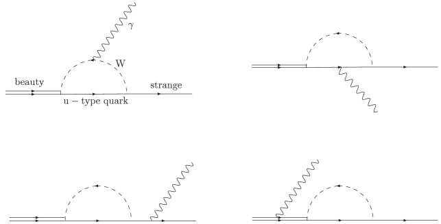
In the rest of this thesis we will deal with the process (3.8): the world average for the experimental branching ratio is [41, 42]

$$BR(B\rightarrow X_{s}\gamma)=(3.34\pm 0.38)10^{-4}$$ (3.11)

In general, inclusive decay rates of the $b$ quark can be calculated in perturbation theory in a model independent way. However exclusive decay rates are easier to measure, though they cannot be calculated from first principles.
Since the exclusive channel $B\rightarrow K\gamma$ violates angular momentum conservation, the simplest process to observe is $B\rightarrow K^{\ast}\gamma$. The first measurement of the exclusive rate for the final states $K^{\ast}(892)\gamma$ has been performed at CLEO [43].
To measure inclusive decay rates two independent methods are used [44]: the cleanest way is to measure and sum decay rates for different exclusive channels as $K\gamma n\pi$ where $n\leq 4$ and at most one pion is a $\pi^{0}$. The previous constraint are necessary to reduce the background but introduce some model dependence.
The previous method can be integrated with an independent one, which consist in measuring of the high energy photon, emitted in the process. The photon spectrum has to be separated from the background of other processes and this is performed by using a neural network. This method was used at CLEO to perform the first measure of the inclusive rate for $b\rightarrow s\gamma$.
Since in the Standard Model flavour changing neutral current do not occur, a decay such as (3.8) must be mediated by a loop even at the lowest level.
As shown in the figure (3.1), the particles in the loop are a virtual W and a virtual u-type quark, that is up, charm or top. The different contribution of the three quarks in the loop is mainly due to the ratio of CKM elements: since $V_{ub}$ is much smaller than $V_{cb}$ and $V_{tb}$ the $u$ quark contribution in the loop can be safely neglected. The $t$ quark is favored by its larger mass, but $c$ quark contribution should not be left out. It turns out to amount about $30\%$.
The photon can be radiated by each charged line, as shown in the figure.
Since this decay is loop mediated it is a sensitive probe of new physics: for example the $W$ boson may be substituted by a charged Higgs, in an extension of the Standard Model with two scalar doublets [49] or by a supersimmetric particle. If the mass of new physics particles is not larger by many order of magnitude than Standard Model particles an effect should be detectable. However it should be pointed out that efforts to find signals of new physics in past years have not given results and, at the moment, the branching ratio for this process agrees with the prediction of the theory.
Recent calculations for the inclusive branching ratio gives the prediction [45, 46]

$$BR(B\rightarrow X_{s}\gamma)=(3.60\pm 0.30)\ 10^{-4}$$ (3.12)

Another useful application of $b\rightarrow s\gamma$ is the measure of CKM elements: in particular this process may provide a way to parametrize non perturbative effects in non perturbative functions that can be used as an input in (3.7), allowing a precise measure of $|V_{ub}|$ [47].
The reason why we are interested in this process is that $b\rightarrow s\gamma$ shows a non trivial interplay between electroweak and strong interactions: the process at quark level is mediated by electroweak interactions, but coloured particles are responsible of gluon emissions which can be treated by well known tools of QCD (resummation, evolution equations, …).
Taking into account QCD corrections different scale appear in the process: $m_{t}\sim m_{W}$ is the mass of the heavy (virtual) particles in the loop, $m_{b}$, the $b$ quark mass, is the hard scale of the process, $\Lambda_{QCD}$ is the scale where non perturbative strong effects appear and they can be ordered as

$$m_{t}\sim m_{W}\gg m_{b}\gg\Lambda_{QCD}$$ (3.13)

The interplay between these scales makes the process difficult to handle: they can be disentangled by building an effective theory where the heavy particles are integrated out and an effective low energy hamiltonian is considered, like in Fermi hamiltonian for $\beta$ decays.
In the next section such an hamiltonian will be briefly described.

3.3 Effective Hamiltonian for $b\rightarrow s\gamma$

QCD corrections to the vertex in figure (3.1) heavily change the lowest order result and need to be handled carefully: due to the presence of different energy scales large logarithms of the form

$$\alpha^{n}_{S}\ \log^{p}(m^{2}_{W}/m^{2}_{b})\ \ \ \rm with\ \ p\leq n$$ (3.14)

make their appearance at higher orders of perturbation theory. These logarithms are significant because $m_{W}\gg m_{b}$ and the term $\frac{\alpha_{S}}{\pi}\log m^{2}_{W}/m^{2}_{b}$ is too large to be a good expansion parameter. Terms such as (3.14) can be resummed with Renormalization Group Equations to take them under control.
This can be done by building an effective hamiltonian of the form [49, 50]

$${\cal H}_{eff}(x)=-{4G_{F}\over\sqrt{2}}\ V^{*}_{ts}V_{tb}\ \sum_{j=1}^{8}C_{j}(\mu_{b})\ \hat{\cal O}_{j}(x;\mu_{b}).$$ (3.15)

This way long-distance effects, both perturbative and non-perturbative, are factorized in the matrix elements of the operators $\hat{\cal O}_{j}$, while the short-distance effects are contained in the coefficient functions $C_{j}(\mu_{b})$, calculable in perturbation theory.
In order to build the effective hamiltonian, the heavy particles in the loop, the $W$ boson and the $top$ quark, have to be integrated out, so that they do not appear as physical degrees of freedom. The integration of the two heavy particles at the same time corresponds to neglect strong coupling running effects between $m_{t}$ and $m_{W}$.
Then the large logarithms are included in the coefficient functions $C_{j}(\mu)$ by scaling down the coefficients to $\mu=O(m_{b})$. Logarithms can be resummed in the coefficients $C_{j}(\mu_{b})$ with the required accuracy: for example the leading approximation involves the resummation of terms with $n=p$, the next-to-leading one terms with $p=n-1$ and so on. This is performed in [49, 51, 52, 53, 54] in $\overline{MS}$ scheme.
At the end, an hamiltonian describing a 5 quark theory is obtained.
A suitable basis for the operators $\hat{\cal O}_{j}$ is given by six four-quark operators,the current-current operators $\hat{\cal O}_{1}$, $\hat{\cal O}_{2}$ and the so called penguin operators $\hat{\cal O}_{3}-\hat{\cal O}_{6}$, and by the magnetic penguin operators (electromagnetic) $\hat{\cal O}_{7}$ and (chromomagnetic) $\hat{\cal O}_{8}$ [49, 50]:

$$\hat{\cal O}_{1} = (\overline{c}_{L,\beta}\gamma_{\mu}b_{L,\alpha})(\overline{s}_{L,\alpha}\gamma_{\mu}c_{L,\beta})$$

$$\hat{\cal O}_{2} = (\overline{c}_{L,\alpha}\gamma_{\mu}b_{L,\alpha})(\overline{s}_{L,\beta}\gamma_{\mu}c_{L,\beta})$$

$$\hat{\cal O}_{3} = (\overline{s}_{L,\alpha}\gamma_{\mu}b_{L,\alpha})(\sum_{q}\overline{q}_{L,\beta}\gamma_{\mu}q_{L,\beta})$$

$$\hat{\cal O}_{4} = (\overline{s}_{L,\alpha}\gamma_{\mu}b_{L,\beta})(\sum_{q}\overline{q}_{L,\beta}\gamma_{\mu}q_{L,\alpha})$$

$$\hat{\cal O}_{5} = (\overline{s}_{L,\alpha}\gamma_{\mu}b_{L,\alpha})(\sum_{q}\overline{q}_{R,\beta}\gamma_{\mu}q_{R,\beta})$$

$$\hat{\cal O}_{6} = (\overline{s}_{L,\alpha}\gamma_{\mu}b_{L,\beta})(\sum_{q}\overline{q}_{R,\beta}\gamma_{\mu}q_{R,\alpha})$$

$$\hat{\cal O}_{7} = {e\over 16\pi^{2}}m_{b,\overline{MS}}(\mu_{b})\overline{s}_{L,\alpha}\sigma^{\mu\nu}b_{R,\alpha}F_{\mu\nu}$$

$$\hat{\cal O}_{8} = {g\over 16\pi^{2}}m_{b,\overline{MS}}(\mu_{b})\overline{s}_{L,\alpha}\sigma^{\mu\nu}T^{a}_{\alpha\beta}b_{R,\alpha}G^{a}_{\mu\nu},$$ (3.16)

where $m_{b,\overline{MS}}(\mu_{b})$ is the $b$ mass in the $\overline{MS}$ scheme, evaluated at $\mu_{b}$ and $q=u,d,s,c$ or $b$. In the operators $\hat{\cal O}_{7}$ and $\hat{\cal O}_{8}$ a term proportional to $m_{s}$ is present, but we have omitted it because $m_{s}\ll m_{b}$ and the approximation $m_{s}\rightarrow 0$ is justified.
For several reasons a different choice for the basis can be performed and we will follow the definition given in [52]. This basis reads

$$\hat{\cal O}_{1} = (\overline{s}_{L}\gamma_{\mu}T^{a}c_{L})(\overline{c}_{L}\gamma^{\mu}T^{a}b_{L})$$

$$\hat{\cal O}_{2} = (\overline{s}_{L}\gamma_{\mu}c_{L})(\overline{c}_{L}\gamma^{\mu}b_{L})$$

$$\hat{\cal O}_{3} = (\overline{s}_{L}\gamma_{\mu}b_{L})(\sum_{q}\overline{q}\gamma^{\mu}q)$$

$$\hat{\cal O}_{4} = (\overline{s}_{L}\gamma_{\mu}T^{a}b_{L})(\sum_{q}\overline{q}\gamma^{\mu}T^{a}q_{L})$$

$$\hat{\cal O}_{5} = (\overline{s}_{L}\gamma_{\mu_{1}}\gamma_{\mu_{2}}\gamma_{\mu_{3}}b_{L})(\sum_{q}\overline{q}\gamma^{\mu_{1}}\gamma^{\mu_{2}}\gamma^{\mu_{3}}q)$$

$$\hat{\cal O}_{6} = (\overline{s}_{L}\gamma_{\mu_{1}}\gamma_{\mu_{2}}\gamma_{\mu_{3}}T^{a}b_{L})(\sum_{q}\overline{q}\gamma^{\mu_{1}}\gamma^{\mu_{2}}\gamma^{\mu_{3}}T^{a}q)$$

$$\hat{\cal O}_{7} = {e\over 16\pi^{2}}m_{b,\overline{MS}}(\mu_{b})\overline{s}_{L,\alpha}\sigma^{\mu\nu}b_{R,\alpha}F_{\mu\nu}$$

$$\hat{\cal O}_{8} = {g\over 16\pi^{2}}m_{b,\overline{MS}}(\mu_{b})\overline{s}_{L,\alpha}\sigma^{\mu\nu}T^{a}_{\alpha\beta}b_{R,\alpha}G^{a}_{\mu\nu}.$$

It is important to underline that (3.3) and (3.3) are equivalent from a physical point of view and can be turned one into other with proper transformations.
The dimension of these operators is six: higher-dimension operators have coefficients suppressed by inverse powers of the masses of the integrated particles ($t$ and $W$) and do not contribute in first approximation.

3.4 Lowest Order Amplitude for $b\rightarrow s\gamma$

Now to calculate the inclusive rate for $b\rightarrow s\gamma$ one has to evaluate the matrix elements of the operators of the basis (3.3) between external states.
Let us consider at first the lowest level. The matrix element for a generic operator $\hat{\cal O}_{i}$ is

$$<s\gamma|\hat{\cal O}_{i}|b>.$$ (3.18)

A straightforward calculation shows that the operators $\hat{\cal O}_{1}$-$\hat{\cal O}_{6}$ have vanishing matrix elements. Moreover the operator $\hat{\cal O}_{8}$ at the lowest level describes the process $b\rightarrow s~{}g$, so that it enters only in radiative corrections.
At the lowest level the only operator giving contribution is $\hat{\cal O}_{7}$, whose matrix element reads

$$<s\gamma|\hat{\cal O}_{7}|b>=m_{b}\frac{e}{8\pi^{2}}\overline{u}(P)\epsilon\!\!/q\!\!\!/\frac{1+\gamma_{5}}{2}u(p)$$ (3.19)

where $\epsilon$ is the photon polarization, $q^{\mu}$ the photon momentum, $P^{\mu}$ and $p^{\mu}$ are respectively the heavy and light quark momenta.
The inclusive rate is

$$\Gamma_{0}=\ |V^{*}_{ts}V_{tb}|^{2}\ \frac{4G_{F}}{m_{b}}\int_{\Phi}\ |<s\gamma|\hat{\cal O}_{7}|b>|^{2}\ d\Phi$$ (3.20)

Let us perform the calculation in the heavy quark rest frame, where

$$P^{\mu}=(m_{b},\vec{0}),$$

for a massless strange quark.
The inclusive rate turns out to be

$$\Gamma_{0}\simeq\frac{\alpha_{em}}{\pi}\frac{G_{F}^{2}\,m_{b}^{3}m_{b,\overline{MS}}^{2}\left(m_{b}\right)\,|V_{tb}V_{ts}^{\ast}|^{2}}{32\pi^{3}}C_{7}^{2}\left(\mu_{b}\right),$$ (3.21)

As we pointed out, the parameter $m_{b}$, appearing in physical results, should be carefully considered: the lowest order rate contains both $m_{b}=m_{b,POLE}$, coming from the phase space, and, in principle, $m_{b,\overline{MS}}(\mu)$, coming from the effective (renormalized) operator [55]. However, as long as QCD corrections are not concerned, the renormalization point is not important and we can safely choose $\mu=m_{b}$. As we will see, when strong interaction are calculated, the definition of the $b$ mass in the $\overline{MS}$ scheme must be coherent with the point where the coefficient functions are evaluated.

3.5 QCD Radiative Corrections for $b\rightarrow s\gamma$

QCD corrections to the process we are considering involve the calculation of Feynman diagrams for real and virtual gluon emissions.
Once the effective hamiltonian is built, one can calculate the n-th order QCD correction to the rate in perturbation theory, by evaluating the contributions of gluon emissions, that is processes such as

$$b\rightarrow s\gamma\ g_{1}\dots g_{n}.$$ (3.22)

This can be accomplished by evaluating the coefficient functions $C_{j}(\mu)$ at the order $\alpha_{S}^{n}$ and the matrix elements

$$<s\gamma g_{1}\dots g_{n}|\hat{O}_{j}|b>$$ (3.23)

for the effective operators. To obtain sensible physical results, these terms must be coherently evaluated in the same renormalization scheme, for example $\overline{MS}$, as usually done in literature. In particular $\alpha_{S}$ corrections to the inclusive rate of $b\rightarrow s\gamma$ are calculated in [56] for gluon brehmsstrahlung and in [57, 58] for virtual diagrams.
Not all the operators of the basis (3.3) give a contribution as relevant as the others to the inclusive rate: it turns out that $\hat{\cal O}_{7}$ is responsible about for 85% of the total rate and the remaining contributions are mainly due to the operators $\hat{\cal O}_{2}$ and $\hat{\cal O}_{8}$. In practice the other operators can be neglected because they are associated to very small coefficient functions or give vanishing amplitudes. One has just to pay some attention to the operators $\hat{\cal O}_{5}$ and $\hat{\cal O}_{6}$, giving non negligible terms, which can be taken into account with a redefinition of the coefficients functions of $C_{7}$ and $C_{8}$ [56, 57, 58]

$$\tilde{C}_{1\dots 6} = C_{1\dots 6}$$

$$\tilde{C}_{7} = C_{7}-\frac{1}{3}C_{5}-C_{6}$$

$$\tilde{C}_{8} = C_{8}+C_{5}.$$ (3.24)

In this way one can mainly consider the operator $\hat{\cal O}_{7}$ and smaller terms given by $\hat{\cal O}_{2}$ and $\hat{\cal O}_{8}$.
The evolution of the coefficient functions $C_{i}^{eff}(\mu)$ is governed by the renormalization group equation

$$\mu\frac{d}{d\mu}C_{i}^{eff}(\mu)=\gamma_{ij}^{eff}(\alpha_{S})C_{j}^{eff}$$ (3.25)

where $\gamma_{ij}^{eff}$ is the anomalous dimension matrix related to the effective coefficient functions defined in (3.5). In recent years, efforts to achieve a next-to-leading accuracy has been done, to reduce the renormalization scale dependence of the amplitude, which was found to be the largest source of uncertainty [48]. This request needs the knowledge of the (effective) coefficient functions up to $O(\alpha_{S})$

$$C_{i}^{eff}=C^{(0)eff}_{i}(\mu)+\frac{\alpha_{S}(\mu)}{4\pi}C^{(1)eff}_{i}(\mu)+O(\alpha_{S})$$ (3.26)

and the anomalous dimension matrix up to $O(\alpha_{S}^{2})$

$$\gamma_{ij}^{eff}=\frac{\alpha_{S}}{4\pi}\gamma^{(0)eff}_{ij}+\left(\frac{\alpha_{S}(\mu)}{4\pi}\right)^{2}\gamma^{(1)eff}_{ij}+O(\alpha^{3}_{S})$$ (3.27)

This huge work has been performed by different groups in the last years and final results are listed in [53, 52] and in references therein.
Further details about the QCD corrections are discussed in the chapters 5 and 7, where explicit calculations are shown. Here let us finally recall the result for the contribution of the leading operator $\hat{\cal O}_{7}$ to the order $\alpha_{S}$ as calculated in [56, 57, 58]:

$$\Gamma_{7} = \Gamma_{0}\tilde{C}_{7}^{2}(\mu)\left[1+\frac{\alpha_{S}}{\pi}\left(\frac{16}{9}-\frac{4}{9}\pi^{2}+\frac{16}{3}\log\frac{m_{b}}{\mu}\right)\right]=$$

$$\Gamma_{7} = \Gamma_{0}\tilde{C}_{7}^{2}(\mu)\left[1+\frac{\alpha_{S}}{\pi}\left(\frac{16}{9}-\frac{4}{9}\pi^{2}+\frac{4}{3}\log\frac{m_{b}}{\mu}\right)\right]\left(\frac{m^{2}_{b,\overline{MS}}(\mu)}{m^{2}_{b,\overline{MS}}(m_{b})}\right).$$

The two expressions in (3.5) reduce one another because of the relation

$$m_{b,\overline{MS}}(\mu)=m_{b,\overline{MS}}(m_{b})\left(1+\frac{2\alpha_{S}(m_{b})}{\pi}\log\frac{m_{b}}{\mu}\right).$$ (3.29)

and can be chosen depending which mass we want in the lowest order amplitude, $m_{b,\overline{MS}}(\mu)$ or $m_{b,\overline{MS}}(m_{b})$.

3.6 Photon Spectrum

The spectrum of the photon is the first distribution calculated and measured for $b\rightarrow s\gamma$.
The kinematics of this process is very simple: at the lowest level it is a two body decay, so that the photon energy is fixed by the kinematics: in the approximation of a massless strange quark the spectrum is discrete and monochromatic and the photon energy is:

$$E_{\gamma}=\frac{m_{b}}{2}.$$ (3.30)

This approximation is obviously too naïve, because it does not take into account two fundamental effects:

• gluon emissions radically change the spectrum, making the process a multi-body decay: the spectrum becomes continuous

  $$0\leq E_{\gamma}\leq E_{\gamma}^{MAX}=\frac{m_{b}}{2}$$ (3.31)

  QCD corrections have to calculated in perturbation theory. As discussed in Chapter 2 an improved perturbative expansion is needed to have reliable results in the whole phase space;

• non perturbative effects play a role: for small exchanged momenta, non perturbative effects make their appearance, related to final states effects (hadronization) and initial state effects (Fermi motion). Obviously they cannot be calculated in perturbation theory and need to be factorized in some fragmentation or structure function. They will be discussed in Chapter 6. They spread the spectrum around the endpoint.

The photon spectrum was first calculated in [59] for a massive strange quark. A comparison with the data present at the time is performed in [55], where a model to deal with the Fermi motion effects is introduced. The comparison, used to extract the ratio $\left|\frac{V_{ts}}{V_{cb}}\right|$, agrees with the prediction of the Standard Model, based on the unitarity triangle. Latest experimental results from CLEO collaboration are shown in [60].

Figure 3.2: Photon spectrum in $b\rightarrow s\gamma$ measured at CLEO [60].

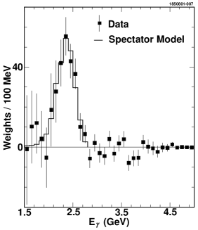
Other details about the photon spectrum will be discussed in section (6.1).
Let us only remark that this is a distribution where large logarithms appear near the border of the phase space, related to emission of infrared gluons. This happens in the region near the endpoint of the photon spectrum, for $E_{\gamma}\rightarrow m_{b}/2$. These large logarithms spoil the perturbative expansion in that region and the usual approach to handle them is their resummation according to the theory described in section (2.11).
In section (5) this will be shown and the limits of this approach will be described.
To conclude let us underline that the photon spectrum has been the first distribution studied for the process we are dealing with: the photon spectrum is sensitive to longitudinal degrees of freedom, along the photon direction. On the contrary the transverse momentum distribution of the strange quark with respect to the photon direction is sensitive to transverse degrees of freedom, so that it can give complementary information about the dynamics of the process.
In Chapter 6 the photon spectrum and the transverse momentum distribution will be compared: being sensitive to different degrees of freedom they can give complementary informations about several features of $b$ physics, such as non perturbative effects, reliability of the perturbative expansion and so on.

Part II Transverse Momentum Distribution in $b\rightarrow s\gamma$

Chapter 4 Preliminary Observations

4.1 Motivations

In the next chapters the calculations concerning the transverse momentum distribution in the rare decay $b\rightarrow s\gamma$ will be discussed and described in great detail. This topic was introduced in [1] and the calculation was completed in [2]: here we want to underline the motivations which induce us to analyze this argument and its relevance in the outline of $b$ physics.
In the last years experiments dedicated to the study of $b$ physics have been set up: in particular BaBar at Fermilab and Belle at KEK began to carry out a wide program of measurements of parameters involved in the physics of this quark. The rich phenomenology of the $b$ physics opens many possibilities both experimentally and theoretically: the final aim remains a precise test of the Standard Model, with the determination of every parameter involved in the predictions of the theory and a compelling comparison with experimental data. This can show the level of accuracy of the theory.
Since the discovery of the $b$ quark the importance of QCD corrections in processes involving it was evident: the tree level process is always mediated by an electroweak current, but emissions of gluon by initial or final quark change radically the theoretical prediction. The most manifest case is just related to $b\rightarrow s\gamma$ which is one of the few processes where radiative corrections have a larger size than the lowest order.
Perturbative QCD was widely applied to the $b$ physics in past years and in particular also to its decays: the $b$ quark is the lightest quark where this kind of approach can be considered viable. Its mass, as discussed in the chapter 3, is larger than the typical scale of hadronization, see eq. (3.4), and the strong coupling constant $\alpha_{S}$ can be considered a good parameter for the perturbative expansion, being reasonably smaller than one [5]:

$$\alpha_{S}(m_{b})\cong 0.22.$$ (4.1)

For lighter quark these considerations are not valid: even the quark $charm$ is too light for a reasonable application of pQCD without heavy corrections.
This has driven to consider perturbative QCD as an essential tool in $b$ decays: in particular also more refined tools of the theory have been applied to this kind of processes, for example the resummation of large logarithms for semi-inclusive observables has become a standard technique.
In the last twenty years QCD has had amazing confirmations of its predictions in experiments of high energy physics, for example at LEP: however in these cases the scale of energy where the processes occurred was much higher with respect to the $b$ decays. Typically these experiments where performed at scales larger than $Z^{0}$ mass,

$$M_{Z^{0}}\cong 91{\rm GeV},$$ (4.2)

where the strong coupling constant is about an half the coupling constant at the $b$ mass energy:

$$\alpha_{S}(M_{Z^{0}})=0.12.$$ (4.3)

Moreover in $b$ physics theoretical prediction are complicated by the presence of parameters in principle unknown and that cannot be extracted by the theory: in particular the CKM matrix elements and the quark mass which, as discussed in Chapter 3, are poorly known. These parameters are affected by uncertainties which can confuse QCD predictions. They are usually eliminated by considering ratio of widths of different processes, which cancel the dependance on the quark mass and in several cases also on CKM matrix elements. A rather good theoretical quantity is represented, for instance, by the semileptonic branching ratio:

$$B_{SL}=\frac{\Gamma_{SL}}{\Gamma_{TOT}},$$ (4.4)

which turns out to be marginally in agreement with present data [61].
These reasons drove us to calculate with high accuracy (next-to-leading level resummation + fixed order hard contributions) a distribution in a decay of the $b$ quark.
The second question to answer is why we decided to study this particular decay, $b\rightarrow s\gamma$: as stated in chapter 3 this is a rare decay, has a small branching ratio, presents many experimental difficulties for the measurements and therefore seems not to be the most immediate choice. However the reasons we have studied it is that has interesting and suitable features: being at the lowest level a two body decay its kinematics is very simple, so that one can face the problem of radiative corrections and resummation without additional and unimportant complications. Moreover the results are in many cases very general and can be extended to other processes such as the semileptonic decay $b\rightarrow u+e+\overline{\nu}_{e}$ or the phenomenologically more important $b\rightarrow c+e+\overline{\nu}_{e}$, where the mass of the final quark is a big kinematical complication.
The tool of resummation was mainly applied, in past years, to processes involving light quarks only, while in this case the presence of an heavy quark in the initial states gives additional and new effects.
In our case this scheme is justified by the fact that the double logarithm appearing to order $\alpha_{S}$ can become rather large (with respect to 1 coming from the tree level):

$$-\frac{\alpha_{S}C_{F}}{4\pi}\log^{2}\frac{p_{t}^{2}}{m_{b}^{2}}\sim-0.7$$ (4.5)

if we push the transverse momentum to such small values as $p_{t}~{}\sim~{}\Lambda_{QCD}~{}=~{}300$ MeV. The single logarithm can also become rather large, having a large numerical coefficient:

$$-\frac{5\alpha_{S}C_{F}}{4\pi}\log\frac{p_{t}^{2}}{m_{b}^{2}}\sim 0.6.$$ (4.6)

The purpose of resumming classes of such terms therefore seems quite justified. If we consider running coupling effects, i.e. if the (frozen) coupling evaluated at the hard scale $Q~{}=~{}m_{B}~{}=~{}5.2$ GeV is replaced by the coupling evaluated at the gluon transverse momentum,

$$\alpha_{S}(m_{b})\rightarrow\alpha_{S}(p_{t})=0.45~{}~{}~{}~{}~{}~{}{\rm{for}}~{}~{}~{}~{}~{}p_{t}~{}=~{}1~{}\rm{GeV},$$ (4.7)

the logarithmic terms have sizes of order:

$$-\frac{\alpha_{S}(p_{t})C_{F}}{4\pi}\log^{2}\frac{p_{t}^{2}}{m_{b}^{2}}\sim-0.5$$ (4.8)

and

$$-\frac{5\alpha_{S}C_{F}}{4\pi}\log\frac{p_{t}^{2}}{m_{b}^{2}}\sim 0.8.$$ (4.9)

The main difference with respect to resummation in $Z^{0}$ decays is a hard scale smaller by over an order of magnitude, i.e. a coupling larger by a factor 2 and infrared logarithms smaller by a factor 3.
Finally this decay, even if rare, has been widely studied experimentally because it seemed to be a privileged process for the discovery of new physics: matter of fact all the discrepancies between experimental data and theoretical predictions could be explained and up to now no signals of new physics have been found. However the large effort to measure this process have produced a huge amount of experimental data, which will be possibly compared with our predictions.
The last question to make clear is why we decide to study the transverse momentum distribution: the main reason is that for this process the photon spectrum has been calculated, measured and the role of non perturbative contributions has been discussed, with the introduction of a structure function, called shape function [62]. The transverse momentum is sensitive to a complementary kinematics with respect to the photon spectrum, so that it can give additional informations about the process.
In the following chapters the calculation of the transverse momentum distribution will be discussed: according to the theory of resummation we decided to achieve a next-to-leading accuracy in the calculation, for the reasons discussed in section (2.11).
This level of accuracy requires the calculation of the coefficient controlling double and single logarithmic effects and the resummation of logarithms in the function $g_{1}$ and $g_{2}$ introduced in section (2.11). This part, the next-to-leading-logarithmic approximation (NLL), is described in Chapter 5.
In order to achieve a complete next-to-leading order accuracy (NLO), hard terms to the order $\alpha_{S}$ have been calculated in Chapter 7, which shows the computation of real and virtual Feynman diagrams to the order $\alpha_{S}$.
The resummation of the transverse momentum show different results with respect to the photon spectrum and a comparison between these two complementary distributions is performed in chapter 6.

4.2 Kinematics

The specific process we are considering is

$$B\rightarrow h_{s}+X+\gamma,$$ (4.10)

where $h_{s}$ is a strange hadron, typically a $K^{\ast}$, and $X$ every other hadronic state. Without any generality loss we can consider the B-meson rest frame and define as reference direction the direction of flight of the photon (axis $+z$).
Let us define the transverse momentum $p_{t}$ of the strange hadron with respect of this direction: it is in practice the projection of the momentum of $h_{s}$ on the plane $x-y$.

Figure 4.1: Kinematics of the transverse momentum distribution.

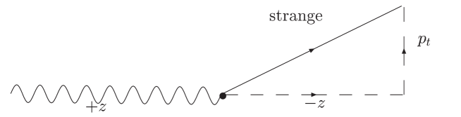
At the lowest order of the partonic level the process is

$$b\rightarrow s+\gamma,$$ (4.11)

so that, being a two body decay, the photon and the strange quark are emitted along the same direction and the transverse momentum, as defined above, vanishes.
However it should be reminded that the physical process that can be detected and measured is the hadronic one (4.10) and radiative corrections change radically the spectrum at the partonic level, so that different sources of transverse momentum can be identified:

• Multiple gluon emissions: the emission of gluons by the initial or the final quark makes the process a multi-body decay

  $$b\rightarrow s\gamma g_{1}\dots g_{n}$$ (4.12)

  and spreads the transverse momentum spectrum. This effect can be calculated order by order in perturbation theory and produce a transverse momentum $p_{p}$ for the strange quark because of momentum conservation.

  

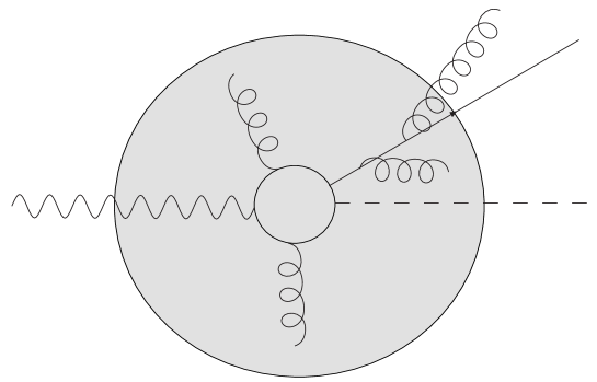
  Figure 4.2: Multiple gluon emission from the initial or the final quark in the heavy quark-meson rest frame.

• Initial state effects: a first non-perturbative effect is the well-known Fermi motion [62]. Classically, this is a small vibratory motion of the $b$ quark in the $B$ meson, caused by the momentum transfer with the valence quark. In the quantum theory, the interaction with the light quark produces also some virtuality of the heavy quark. Let us work in the $B$ rest frame. We can parametrize the heavy quark momentum as:

  $$p_{b}=m_{B}v+p_{f}.$$ (4.13)

  $v^{\mu}$ is the velocity of the heavy quark,

  $$v^{\mu}=(1;0,0,0)$$ (4.14)

  and $p_{f}$ is the residual momentum associated to the Fermi motion, such that

  $$|p_{f}^{\mu}|\sim\Lambda.$$ (4.15)

  where $\Lambda$ is the QCD scale. We expect that Fermi motion produces a distribution of intrinsic transverse momenta of the $b$ quark of order

  $$|p_{f}|\sim\Lambda.$$ (4.16)

  Roughly speaking, we may say that transverse momenta distributions in the region

  $$|p_{t}|\sim\Lambda$$ (4.17)

  are sensitive to the oscillations of the heavy quark in the transverse plane (x , y).

  

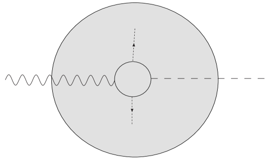
  Figure 4.3: Sketch of Fermi Motion effects on the transverse momentum.

• Final state effects: a second non-perturbative effect is the fragmentation of the strange quark into the hadron $h_{s}.$ According to the idea of local parton-hadron duality, hadronization is expected to modify the partonic distribution by a quantity of the order of the QCD scale:

  $$|p_{h}|\sim\Lambda.$$ (4.18)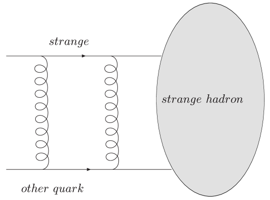

  

  Figure 4.4: Sketch of the effects of the hadronization on the transverse momentum.

The total transverse momentum can be written as the sum of the perturbative and non-perturbative components:

$$p_{t}=p_{p}+p_{f}+p_{h}.$$ (4.19)

and the distribution is controlled by perturbative effects only as long as $|p_{t}|\rm\gg\Lambda_{QCD}$.
Let us note that initial and final state effects involve momenta of the same order and in principle they cannot be separated by any energy scale.

4.2.1 Kinematics for Single Gluon Emission

Let us consider the kinematics at the partonic level for one gluon emission, described in figure (4.5).
The mass of the strange quark can be neglected.
Let us define the fraction of energy of the gluon as

$$\omega=\frac{2E_{g}}{Q}=\frac{2E_{g}}{m_{b}},$$ (4.20)

being the quark mass $m_{b}$ the hard scale of the process.
Let us define as angular variable

$$t=\frac{1-\cos\theta}{2},$$ (4.21)

where $\theta$ is defined as the angle between the opposite of the photon direction (axis -z) and the strange quark direction, as shown in the figure.
$\omega$ and $t$ are unitary variables and the Born kinematics (vanishing transverse momentum) is achieved for $\omega\rightarrow 0$ or $t\rightarrow 0$.

Figure 4.5: Kinematics for one gluon emissions.

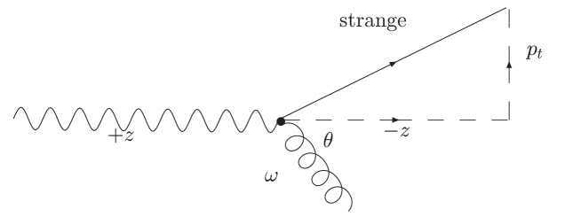
The transverse momentum $p_{t}$ (since now this symbols will denote the modulus of the transverse momentum) of the strange quark can be expressed in terms of these two unitary variables: since $\vec{p}_{t}=-\vec{k}_{t}$, being $\vec{k}_{t}$ the transverse momentum of the gluon, because of momentum conservation, it can be obtained from geometrical considerations that

$$p^{2}_{t}=k^{2}_{t}=m^{2}_{b}\left(\omega^{2}t(1-t)\right).$$ (4.22)

Let us define the adimensional variable

$$x=\frac{p^{2}_{t}}{m^{2}_{b}},$$ (4.23)

so that the kinematical constraint (see section (2.10)) turns out to be

$$\delta\left[x-o(\omega,t)\right]=\delta\left[x-\omega^{2}t(1-t)\right].$$ (4.24)

This kinematical constraint is infrared safe, according to the definition given in section (2.10), since it vanishes in the soft and in the collinear limit:

$$o(\omega,t)\rightarrow 0\ \ \ {\rm for} \ \ \ \omega\rightarrow 0$$

$$o(\omega,t)\rightarrow 0\ \ \ {\rm for} \ \ \ t\rightarrow 0.$$ (4.25)

It turns out from kinematics that the limits on $x$ are

$$0\leq x\leq\frac{1}{4}.$$ (4.26)

Chapter 5 Resummation of Transverse Momentum Distribution

This Chapter is dedicated to the resummation with next-to-leading order accuracy of the large logarithms appearing in the transverse momentum distribution near the border of the phase space.
The first step is the calculation of the coefficients controlling the double and single logarithms.
Then they are resummed to every order by introducing the impact parameter space [33], according to the theory outlined in section (2.11).

5.1 Calculation of the Coefficients $A_{1}$ and $B_{1}$

In this section the distribution of transverse momentum of the strange quark with respect to the photon direction is calculated with logarithmic accuracy for one gluon emission. The partonic process is

$$b\rightarrow s+\gamma+g$$ (5.1)

This computation involves the coefficients $A_{1}$ and $B_{1}$ which control the leading and next-to-leading contributions in the resummed distribution.
As defined in section (4.2.1) we consider the variable :

$$x\equiv{\frac{p_{t}^{2}}{Q^{2}}}\hskip 28.45274pt,\hskip 28.45274ptQ=m_{b}$$ (5.2)

The distribution of interest is therefore:

$$d\left(x\right)=\frac{1}{\Gamma_{0}}\frac{d\Gamma}{dx}.$$ (5.3)

The kinematical constraint to impose on the radiative gluon is given in (4.24)

$$o(\omega,t)=\omega^{2}t(1-t),$$

so that $p_{t}$ distribution is infrared safe.
The aim of this section is the determination of the logarithmic structure at one loop: in order to extract the logarithms arising at this stage the kinematical constraint (4.24) can be expressed with its lowest order approximation

$$\tilde{o}\left(\omega,t\right)=\omega^{2}t.$$ (5.4)

Using the decomposition of the matrix element discussed in section (2.10) (see eq. (2.91)) we can write to the order $\alpha_{S}$:

$$d(x)=\delta(x)+\alpha_{S}\int_{0}^{1}d\omega\int_{0}^{1}dt\left[{\frac{A_{1}}{\omega t}}+{\frac{S_{1}(t)}{\omega}}+{\frac{C_{1}(\omega)}{t}}\right]\left[\delta(x-\omega^{2}t)-\delta(x)\right].$$ (5.5)

The first $\delta$-function describes the real emissions, while the second one describes the virtual emissions. The function $F_{1}$ introduced in (2.91) can be neglected because it does not produce any logarithmic enhancement: it will be taken into account in Chapter (7).
By integrating over the gluon energy and polar angle one obtains the following contributions :

• leading double-logarithmic term:
  

  $$\alpha_{S}A_{1}\int_{0}^{1}\frac{d\omega}{\omega}\int_{0}^{1}\frac{dt}{t}[\delta(x-\omega^{2}t)-\delta(x)]=-{\frac{\alpha_{S}A_{1}}{2}}\left({\frac{\log x}{x}}\right)_{+};$$ (5.6)

• next-to-leading soft term:

  $$\alpha_{S}\int_{0}^{1}dt\int_{0}^{1}d\omega{\frac{S_{1}(t)}{\omega}}[\delta(x-\omega^{2}t)-\delta(x)]={\frac{\alpha_{S}S_{1}}{2}}\left({\frac{1}{x}}\right)_{+}+\mathcal{O}(1);$$ (5.7)

• next-to-leading collinear term:

  $$\alpha_{S}\int_{0}^{1}d\omega\int_{0}^{1}dt{\frac{C_{1}(\omega)}{t}}[\delta(x-\omega^{2}t)-\delta(x)]=\alpha_{S}\,C_{1}\left({\frac{1}{x}}\right)_{+}+\mathcal{O}\left(\frac{1}{\sqrt{x}}\right).$$ (5.8)

Let us underline that the collinear term has a different rest with respect to the soft one: this rest is divergent for $x\rightarrow 0$ even if it does not give rise logarithmic enhancement.
By summing the contributions, the one soft-gluon emission distribution reads:

$$f(x)=\delta(x)-\frac{\alpha_{S}A_{1}}{2}\left({\frac{\log x}{x}}\right)_{+}+\alpha_{S}B_{1}\left(\frac{1}{x}\right)_{+}$$ (5.9)

where

$$B_{1}=C_{1}+{\frac{S_{1}}{2}}=-{\frac{5}{4}}{\frac{C_{F}}{\pi}}$$ (5.10)

In usual hard processes, such as DIS and DY, $S_{1}=0$ so that $B_{1}=C_{1}$. In our case, single logarithmic effects are more pronounced because this coefficient is almost factor 2 larger.

5.2 Exponentiation in the Impact Parameter Space

In this section we are going to deal with the resummation of multiple soft gluon emission: this is performed by factorizing QCD amplitudes for multiple soft gluon emission and introducing the impact parameter space which factorizes the kinematical constraint for transverse momentum [33, 36, 37, 34, 35]. After that one gets the exponentiation of one gluon distribution.
Before dealing with the general case, let us treat in some detail the simplest non-trivial case, namely double emission.

$$b\rightarrow s+\gamma+g_{1}+g_{2}$$ (5.11)

According to transverse momentum conservation we have

$$p_{t}=-{k}_{t1}-k_{t2}.$$ (5.12)

Multi-gluon amplitudes factorize in the infrared limit at leading level, so that

$$\frac{1}{\Gamma_{B}}\frac{d^{2}\Gamma_{2}}{d{k}_{t1}d{k}_{t2}}\left({k}_{t1},k_{t2}\right)\simeq\frac{1}{2}\frac{1}{\Gamma_{B}}\frac{d\Gamma_{1}\left({k}_{t1}\right)}{d{k}_{t1}}\frac{1}{\Gamma_{B}}\frac{d\Gamma_{1}\left({k}_{t2}\right)}{d{k}_{t2}}.$$ (5.13)

where $k_{1}$ and $k_{2}$ are gluons momenta, while $\Gamma_{i}$ is the width of one gluon emission process.
The distribution therefore reads:

$$\frac{1}{\Gamma_{0}}\frac{d\Gamma}{dp_{t}}\left(p_{t}\right) = \delta\left(p_{t}\right)+\int dp_{t1}\delta\left(p_{t}+k_{t1}\right)\frac{1}{\Gamma_{0}}\frac{d\Gamma_{1}\left(k_{t1}\right)}{d{k}_{t1}}+$$ (5.15)

$$+\frac{1}{2}\int d{k}_{t1}k_{t2}\delta\left(p_{t}+{k}_{t1}+{k}_{t2}\right)\frac{1}{\Gamma_{0}}\frac{d\Gamma_{1}\left({k}_{t1}\right)}{d{k}_{t1}}\frac{1}{\Gamma_{0}}\frac{d\Gamma_{1}\left({k}_{t2}\right)}{d{k}_{t2}}+\cdots.\quad$$

The quark transverse momentum distribution is inclusive with respect to gluon radiation: we do not detect the transverse momenta of individual gluons, but only their sum, in an indirect way, by detecting the transverse momentum of the light quark. To solve the $k_{t}$-constraint, we go to the distribution in impact parameter space $b$ by taking a two-dimensional Fourier transform,

$${1\over\Gamma_{0}}\frac{d\widetilde{\Gamma}}{d{b}}\left({b}\right)\equiv\int_{-\infty}^{+\infty}\int_{-\infty}^{+\infty}d{p_{t}}\exp\left[i{p_{t}}\cdot{b}\right]\,{1\over\Gamma_{0}}\frac{d\Gamma\left({p_{t}}\right)}{d{p_{t}}}.$$ (5.16)

Inserting eq. (5.15) in the r.h.s. of eq. (5.16), one obtains

$$\frac{1}{\Gamma_{0}}\frac{d\widetilde{\Gamma}}{d{b}}\left({b}\right) = 1+\frac{1}{\Gamma_{0}}\frac{d\widetilde{\Gamma}_{1}}{d{b}}\left({b}\right)+\frac{1}{2}\left[\frac{1}{\Gamma_{0}}\frac{d\widetilde{\Gamma}_{1}}{d{b}}\left({b}\right)\right]^{2}.$$ (5.17)

Let us now consider the general case. The transverse momentum distribution can be written as

$$\frac{1}{\Gamma_{0}}\frac{d\Gamma}{d{p}_{t}}\left({p}_{t}\right)=\delta\left({p}_{t}\right)+\sum_{n=1}^{\infty}\frac{1}{\Gamma_{0}}\frac{d\Gamma^{\left(n\right)}}{d{p}_{t}}\left({p}_{t}\right),$$ (5.18)

where the distribution due to $n$ real gluons is given by

$$\frac{d\Gamma^{\left(n\right)}}{d{p}_{t}}\left({p}_{t}\right)=\int_{-\infty}^{+\infty}\prod_{l=1}^{n}d{k}_{tl}\frac{d^{n}\Gamma\left({k}_{t1},{k}_{t2},\cdots{k}_{tn}\right)}{d{k}_{t1}d{k}_{t2}\cdots d{k}_{tn}}\delta\left({p}_{t}+{k}_{t1}+{k}_{t2}+\cdots+{k}_{tn}\right).$$ (5.19)

In the infrared limit, the matrix elements for multiple emission factorize into the single emission ones, so that

$$\frac{1}{\Gamma_{0}}\frac{d^{n}\Gamma_{n}\left({k}_{t1},{k}_{t2},\cdots{k}_{tn}\right)}{d{k}_{t1}d{k}_{t2}\cdots d{k}_{tn}}\simeq\frac{1}{n!}\prod_{l=1}^{n}\frac{1}{\Gamma_{0}}\frac{d\Gamma_{1}}{d{k}_{tl}}\left({k}_{tl}\right).$$ (5.20)

The factorization of the amplitudes represented by eq. (5.20) is a dynamical property of QCD. By substituting eq.(5.19) into (5.20) and (5.18) into (5.19), we obtain:

$$\frac{1}{\Gamma_{0}}\frac{d\Gamma\left(p_{t}\right)}{dp_{t}}=\delta\left(p_{t}\right)\,+\,\sum_{n=1}^{\infty}\,\frac{1}{n!}\,\int_{0}^{Q}\,\prod_{l=1}^{n}d^{2}k_{tl}\,\frac{1}{\Gamma_{0}}\frac{d\Gamma_{1}\left(k_{tl}\right)}{dk_{tl}}\,\delta\left(p_{t}+k_{t1}+k_{t2}+\cdots+k_{tn}\right).$$ (5.21)

Substituting eq. (5.20) in eq. (5.16), we obtain the exponentiation of the effective one-gluon distribution in impact parameter space:

$$\frac{1}{\Gamma_{0}}\frac{d\widetilde{\Gamma}}{d{b}}\left({b}\right) = 1+\frac{1}{\Gamma_{0}}\frac{d\widetilde{\Gamma}_{1}}{d{b}}\left({b}\right)+\frac{1}{2}\left[\frac{1}{\Gamma_{0}}\frac{d\widetilde{\Gamma}_{1}}{d{b}}\left({b}\right)\right]^{2}+\cdots$$ (5.22)

$$\stackrel{{\scriptstyle{\rm i.r.\ limit}}}{{=}} \exp\left[\frac{d\widetilde{\Gamma}_{1}}{d{b}}\left({b}\right)\right].$$

The original distribution in momentum space is recovered by an inverse transform,

$$\frac{d\Gamma\left(p_{t}\right)}{dp_{t}}=\int\frac{db}{4\pi^{2}}\exp\left[-ip_{t}\cdot b\right]\frac{d\widetilde{\Gamma}}{db}\left(b\right).$$ (5.23)

Let us stress that the exponentiation of the one-gluon distribution is a consequence of two different facts:

1. Factorization of QCD amplitudes in the infrared limit;

2. Factorization of the kinematical constraint going to impact parameter space.

5.3 Higher orders

In order to achieve a next-to-leading logarithmic resummation higher order effects have to be taken into account. This can be performed by considering the two following prescriptions during the calculation:

1. the bare coupling have to be substituted with a running coupling at two loop level evaluated at transverse momentum squared of the gluon [29]:

   $$\alpha_{S}\rightarrow\alpha_{S}(k_{t}^{2}={p_{t}}^{2})=\alpha_{S}(Q^{2}x),$$ (5.24)

   where the running coupling constant is evaluated with next-to-leading accuracy, according to equation (2.55),

   $$\alpha^{NLO}_{S}(Q^{2}x)={\frac{1}{\beta_{0}}}{\frac{1}{\log({s\,}x)}}-{\frac{\beta_{1}}{\beta_{0}^{3}}}{\frac{\log[\log({s\,}x)]}{\log^{2}({s\,}x)}+O}\left(\beta_{1}^{2}\right){.}$$ (5.25)

   $s$ is defined as:

   $$s\equiv\frac{Q^{2}}{\Lambda^{2}}.$$ (5.26)

   The first two coefficients of the $\beta$-function, $\beta_{0}$ and $\beta_{1},$ are independent of the renormalization scheme (they are universal) and have the values:

   $$\beta_{0}={\frac{33-2n_{f}}{12\pi},\qquad}\beta_{1}={\frac{153-19n_{f}}{24\pi^{2}},}$$ (5.27)

   where $n_{f}=3$ is the number of active flavours. The coupling depends on the transverse momentum only, therefore the integration over energy and angle in equation (5.5) does not involve any running of the coupling; it is sufficient to make the substitution (5.24) in (5.5).

2. the two loop contribution in the double logarithmic term need to be included:

   $$A_{1}\alpha_{S}\rightarrow A_{1}\alpha_{S}+A_{2}\alpha_{S}^{2}.$$ (5.28)

   where the universal coefficient $A_{2}$ is [36]

   $$A_{2}={C_{F}\over 2\pi^{2}}[C_{A}({67\over 18}-{\pi^{2}\over 6})-{5\over 9}\ n_{f}].$$ (5.29)

   According to what stated in the first point one can simply substitute (5.28) in (5.5).

In general the resummation of transverse momentum logarithms involves the following two functions, both possessing power series expansion in $\alpha_{S}$:

$$A\left(\alpha_{S}\right) = \sum_{n=1}^{\infty}A_{n}\,\alpha_{S}^{n}=A_{1}\alpha_{S}+A_{2}\alpha_{S}^{2}+\cdots,$$ (5.30)

$$B\left(\alpha_{S}\right) = \sum_{n=1}^{\infty}{B}_{n}\,\alpha_{S}^{n}={B}_{1}\alpha_{S}+\cdots,$$ (5.31)

5.4 Resummation of the Transverse Momentum Distribution

In this section we will show the results about the resummation of transverse momentum distribution: the results shown here are based on [1].
In order to perform the resummation with next-to-leading accuracy we must follow the prescription in section (5.3): by substituting (5.24) and (5.28) equation (5.5) reads

$$d(x) = \delta(x)+\alpha^{NLO}_{S}(Q^{2}x)\int_{0}^{1}d\omega\int_{0}^{1}dt\left[{\frac{A_{1}+\alpha^{NLO}_{S}(Q^{2}x)A_{2}}{\omega t}}\right.+$$ (5.32)

$$+ {\frac{S_{1}(t)}{\omega}}+\left.{\frac{C_{1}(\omega)}{t}}\right]\left[\delta(x-\omega^{2}t)-\delta(x)\right]$$

After the integration over the phase space we obtain the effective distribution of a single gluon in the transverse momentum space, accurate to the next-to-leading level:

$$d_{R}(x)=-{\frac{A_{1}}{2\beta_{0}}}{\frac{\log x}{x\log sx}}+{\frac{A_{1}\beta_{1}}{2\beta_{0}^{3}}}{\frac{\log x\log\log sx}{x\log^{2}sx}}+{\frac{B_{1}}{\beta_{0}}}{\frac{1}{x\log sx}}-{\frac{A_{2}}{2\beta_{0}^{2}}}{\frac{\log x}{x\log^{2}sx}.}$$ (5.33)

The inclusion of virtual diagrams introduces ”+” distributions.
The resummation of transverse momentum is performed in the impact parameter space [33, 36].
In the impact parameter space the general formula (2.127) becomes

$$\frac{1}{\Gamma_{0}}\frac{d\tilde{\Gamma}}{db}=K\left(\alpha_{S}\right)\,\Sigma\left(b;\alpha_{S}\right)+R\,\left(b;\alpha_{S}\right)$$ (5.34)

Let us define:

$$\overline{d}(b)\equiv\frac{1}{\Gamma_{0}}\frac{d\widetilde{\Gamma}}{db}\left(b\right).$$ (5.35)

Let us recall two important mathematical properties of (5.35): it is real and it depends only on $|b|$.
Now we use the relation

$$\frac{1}{\Gamma_{0}}\frac{d\Gamma\left(p_{t}\right)}{dp_{t}}=\frac{1}{\pi}\frac{1}{\Gamma_{0}}\frac{d\Gamma}{{dp_{t}}^{2}}=\frac{1}{\pi Q^{2}}\frac{1}{\Gamma_{0}}d\left(x\right)$$ (5.36)

and substitute it in the equation (5.16):

$$\overline{d}(b)=\int_{0}^{1}dx\,d(x)\int_{0}^{2\pi}\frac{d\phi}{2\pi}\ \exp\left[iQb\sqrt{x}\cos\phi\right]\,,$$ (5.37)

By combining equations (2.99) and (5.37), and integrating over the azimuthal angle, one obtains

$$\overline{d}(b)=1+\int_{0}^{1}dx\,\,d_{R}(x)\,[J_{0}(Qb\sqrt{x})-1].$$ (5.38)

$J_{0}(s)$ is the Bessel function of zero order defined by the integral

$$J_{0}(s)\equiv\int_{0}^{2\pi}\frac{d\phi}{2\pi}\exp\left[is\,\cos\phi\right],$$ (5.39)

from which follows that $J_{0}(0)=1,$ so that the infrared singularity in $x=0$ is screened.
As shown in section (5.2), by iterating for the multiple gluon emission, the single emission term exponentiate and we obtain

$$\Sigma(b)=\exp\left\{\int_{0}^{1}dx\,\,d_{R}(x)\,[J_{0}(Qb\sqrt{x})-1]\right\}.$$ (5.40)

where the meaning of the function $\Sigma(b)$, is described in section (2.11).
In order to integrate over the $x$ variable, the transverse momentum, we use the following approximation of the Bessel function [36], such an approximation remains valid up to the next-to-leading level:

$$J_{0}(s)-1\simeq-\Theta(s-b_{0})$$ (5.41)

where $b_{0}=2e^{-\gamma_{E}}\approx 1.12.$ We have therefore:

$$\Sigma(b)\simeq\exp\left[-\int_{b_{0}^{2}/\left(Q^{2}b^{2}\right)}^{1}\,d_{R}\left(x\right)\,dx\right].$$ (5.42)

Where $\theta\left(b/b_{0}-1/Q\right)$ in front of the integral is understood. The impact parameter distribution coincides with the cumulative distribution (2.79) in the transverse momentum space. It is important to notice that the step approximation in equation (5.41) cuts the small transverse momenta region, since implies

$$k_{t}^{2}>\frac{b_{0}^{2}}{b^{2}}.$$ (5.43)

Figure 5.1: Plot of the function $f(b)$ in the variable $y=Q^{2}b^{2}/b_{0}^{2}$ $(\alpha_{S}=0.22)$ Solid line: NLO; dotted line: LO.

The approximation (5.41) is therefore equivalent to a prescription for the non perturbative effects related to the infrared pole in the coupling. To order $\alpha_{S},$ one has:

$$\Sigma(b)=\exp\left[\int_{b_{0}^{2}/\left(Q^{2}b^{2}\right)}^{1}dx\left(\frac{1}{2}A_{1}\alpha_{S}{\frac{\log x}{x}}-B_{1}\alpha_{S}{\frac{1}{x}}\right)\right]$$ (5.44)

By integrating over $x$ one obtains:

$$\Sigma(b)=\exp\left[-{A_{1}\over 4}\alpha_{S}\log^{2}\left(\frac{Q^{2}b^{2}}{b_{0}^{2}}\right)-B_{1}\alpha_{S}\log\left(\frac{Q^{2}b^{2}}{b_{0}^{2}}\right)\right].$$ (5.45)

In order to obtain the resumed distribution in impact parameter to every order let us define $d_{R}$ as in eq.(5.33) and substitute it in the eq.(5.42). Then let us integrate over $x$ and write the hard scale logarithm as a function of two loop coupling, by using the equation

$$\log s={\frac{1}{\beta_{0}\alpha_{S}}}+{\frac{\beta_{1}}{\beta_{0}^{2}}}\log\left(\beta_{0}\alpha_{S}\right).$$ (5.46)

The impact parameter resummed distribution may be written as the exponential of a series of functions, as discussed in section (2.11):

$$\Sigma(b)=\exp\left[L\,g_{1}(\beta_{0}\alpha_{S}L)+g_{2}(\beta_{0}\alpha_{S}L)+\alpha_{S}\,g_{3}(\beta_{0}\alpha_{S}L)+\cdots\right]$$ (5.47)

where

$$L\equiv\log\frac{Q^{2}b^{2}}{b_{0}^{2}}$$ (5.48)

and $\alpha_{S}\equiv\alpha_{S}(Q^{2})$.
We obtain the following expressions for the $g_{1}(\omega)$ and $g_{2}(\omega)$ functions:

$$g_{1}(\omega) = {\frac{A_{1}}{2\beta_{0}}}\frac{1}{\omega}\left[\omega+\log(1-\omega)\right],$$ (5.49)

$$g_{2}(\omega) = {-\frac{A_{2}}{2\beta_{0}^{2}}}\left[{\frac{\omega}{1-\omega}}+\log(1-\omega)\right]+$$ (5.50)

$$+ {\frac{A_{1}\beta_{1}}{2\beta_{0}^{3}}}\left[{\frac{\omega}{1-\omega}}+{\frac{\log(1-\omega)}{1-\omega}}-{\frac{1}{2}}\log^{2}(1-\omega)\right]-{\frac{B_{1}}{\beta_{1}}}\log(1-\omega).$$

The expansion to order $\alpha^{2}_{S}$ of the exponent reads:

$$\log\Sigma(b;\alpha_{S})=-{1\over 4}A_{1}\alpha_{S}L^{2}-B_{1}\alpha_{S}L-{1\over 6}A_{1}\beta_{0}\alpha_{S}^{2}L^{3}-{1\over 4}A_{2}\alpha_{S}^{2}L^{2}-{1\over 2}B_{1}\beta_{0}\alpha_{S}^{2}L^{2}$$ (5.51)

Let us note that a single constant $B_{1}$ controls the single-logarithmic effects in any order. The physical reason is that a soft gluon and a collinear one with the same transverse momenta are emitted with the same effective coupling $\alpha_{S}(k^{2}_{\perp})$.
The function $\Sigma(b,\alpha_{S})$ is plotted in fig. (5.1).
It resum the logarithmic enhancements and becomes singular when

$$\omega\rightarrow 1^{-}$$ (5.52)

Since

$$\omega=\beta_{0}\alpha_{S}L\approx\frac{\log Q^{2}b^{2}}{\log Q^{2}/\Lambda^{2}},$$ (5.53)

the singularity occurs when the transverse strange momentum becomes as small as the hadronic scale,

$$p_{\perp}\approx\frac{1}{b}\approx\Lambda.$$ (5.54)

The singularity (5.52) is produced by the infrared pole (Landau pole) in the running coupling and signals an intrinsic limitation of resummed perturbation theory, in agreement with previous qualitative analysis. Let us note that the function $g_{2}$ has basically a pole singularity in the limit (5.52), while $g_{1}$ has only a softer, logarithmic, singularity.

Chapter 6 Comparison between Transverse Momentum Distribution and Threshold Distribution

6.1 The Threshold Distribution

For the rare decay $b\rightarrow s\gamma$ the first distribution to be studied was the threshold distribution, that is the spectrum of the jet invariant mass and it is strictly related by the kinematics to the photon spectrum , so that in practice they are the same quantity.
This distribution is particularly interesting both experimentally and theoretically near the endpoint of the spectrum, namely where

$$E_{\gamma} = \frac{m_{b}}{2}$$

$$m^{2}_{X} \rightarrow 0.$$ (6.1)

The theoretical importance lies on the appearance of interesting effects of logarithmic enhancement near the endpoint, which drove to apply techniques of resummation in $b$ physics. Moreover in the endpoint region non perturbative effects become relevant and the interplay between resummed perturbative distribution and non perturbative bound state effects turns out to be crucial to understand.
From the experimental point of view physicists studying rare decays such as $b\rightarrow s\gamma$ or $b\rightarrow ue^{-}\overline{\nu}_{e}$ have to face the problem of the large background coming from the transition $b\rightarrow c$, which is overwhelming in almost the whole phase space. Since the mass of the quark $charm$ cannot be neglected in the process

$$b\rightarrow ce^{-}\overline{\nu}_{e}$$ (6.2)

it turns out that the endpoint of the electron spectrum is reached for

$$E^{b\rightarrow c}_{e}=\frac{m^{2}_{b}-m^{2}_{c}}{2m_{b}},$$ (6.3)

so that in the endpoint region of the electron spectrum for $b\rightarrow u$

$$E^{b\rightarrow u}_{e}=\frac{m_{b}}{2}$$ (6.4)

the dominant transition $b\rightarrow c$ is forbidden and its background eliminated.
An analogous problem appear for $b\rightarrow s\gamma$, where the annoying background is due to radiative photon emissions from the tower of transitions $b\rightarrow c\rightarrow s$ and one has to discriminate from strange hadrons coming from the process of interest and the ones coming from charm quark decays. However in the endpoint, for

$$E_{\gamma}>\frac{m^{2}_{b}-m^{2}_{c}}{2m_{b}},$$ (6.5)

again the dominant transition is forbidden and the spectrum of $b\rightarrow s\gamma$ can be cleanly measured.
Results about fixed order calculations [59] and resummed calculations [63] has been performed for this distribution in past years and non perturbative effects has been included by defining a structure function, called shape function [62], based on the heavy quark effective theory [64].
In this chapter these results will be compared with the analogous ones found for the transverse momentum distribution, showing peculiar differences between these two quantities.

6.2 Threshold distribution at Order $\alpha_{S}$

Let us consider the energy spectrum of the photon in the rare decay $b\rightarrow s\gamma$ near the endpoint:

$$f(z)=\frac{1}{\Gamma_{0}}\frac{d\Gamma}{dz}$$ (6.6)

with

$$z\equiv\frac{2E_{\gamma}}{m_{B}}=1-\frac{m_{X}^{2}}{m_{B}^{2}}.$$ (6.7)

The photon spectrum then coincides with the mass distribution of the jet. The kinematic constraint is:

$$o\left(\omega,t\right)=\omega t.$$ (6.8)

Let us note that it is infrared safe. Explicitly the distribution reads

$$f(z)=\delta(1-z)+\alpha_{S}\int_{0}^{1}d\omega\int_{0}^{1}dt\left[{\frac{A_{1}}{\omega t}}+{\frac{S_{1}(t)}{\omega}}+{\frac{C_{1}(\omega)}{t}}\right]\left[\delta(1-z-\omega t)-\delta(1-z)\right].$$ (6.9)

By integrating over the energy and the polar angle we obtain:

$$f(z)=\delta(1-z)-\alpha_{S}A_{1}\left({\frac{\log\left[1-z\right]}{1-z}}\right)_{+}+B_{1}\alpha_{S}\left({\ \frac{1}{1-z}}\right)_{+},$$ (6.10)

where the finite corrections have been neglected and we have defined

$$B_{1}=S_{1}+C_{1}.$$ (6.11)

Note the symmetry between the variables $\omega$ e $t$ implying that the coefficient of the next-to-leading term is the sum of the soft and the collinear coefficient and so it is for $\omega\leftrightarrow t$ symmetries. Large infrared contributions are included by replacing the bare coupling with the running coupling constant evaluated at the transverse momentum squared

$$\alpha_{S}\rightarrow\alpha_{S}k_{t}^{2},$$ (6.12)

where

$$k_{t}^{2}\simeq Q^{2}\omega^{2}t.$$ (6.13)

Here the symmetry between soft and collinear contributions starts to be broken.

6.3 Resummation of the Threshold Distribution

In this case the resummation can be performed in Mellin space:

$${\frac{1}{\Gamma_{0}}}\ \Gamma_{N}=\int_{0}^{1}\ dx\ x^{N-1}{\frac{1}{\Gamma_{0}}}\ {\frac{d\Gamma}{dx}}$$ (6.14)

The general formula (2.127) for the N-th moment of the rate can be written as [38, 39],

$$\frac{1}{\Gamma_{0}}\ \Gamma_{N}=\mathcal{C}\left(\alpha_{S}\right)\,f_{N}\left(\alpha_{S}\right)+R_{N}\left(\alpha_{S}\right),$$ (6.15)

where now the large logarithm contains the $N$-variable:

$$\qquad\qquad\qquad\qquad L\equiv\log\frac{N}{N_{0}}\qquad\qquad\left(\mathrm{threshold\,\,case}\right),$$ (6.16)

with $N_{0}\equiv\exp\left[-\gamma_{E}\right].$ The functions $g_{i}$ in the exponent are different with respect to the ones in the $p_{\perp}$ case and the leading and next-to-leading ones read [63, 65]:

$$g_{1}\left(\lambda\right) = -{\frac{A_{1}}{2\beta_{0}}}\frac{1}{\lambda}\left[(1-2\lambda)\log(1-2\lambda)-2(1-\lambda)\log(1-\lambda)\right],$$

$$g_{2}\left(\lambda\right) = \frac{\beta_{0}A_{2}-\beta_{1}A_{1}}{2\beta_{0}^{3}}\left[\log(1-2\lambda)-2\log(1-\lambda)\right]-\frac{\beta_{1}A_{1}}{4\beta_{0}^{3}}\left[\log^{2}(1-2\lambda)-2\log^{2}(1-\lambda)\right]+$$ (6.17)

$$+\frac{S_{1}}{2\beta_{0}}\log(1-2\lambda)+\frac{C_{1}}{\beta_{0}}\log(1-\lambda).$$

The expansion to order $\alpha_{S}^{2}$ of the exponent reads:

$$\log f_{N}=-\frac{1}{2}A_{1}\alpha_{S}{L}^{2}-\alpha_{S}\left(S_{1}+C_{1}\right)\,{L}-\frac{1}{2}A_{1}\beta_{0}\alpha_{S}^{2}L^{3}-\frac{1}{2}A_{2}\alpha_{S}^{2}L^{2}-\left(S_{1}+\frac{1}{2}C_{1}\right)\beta_{0}\,\alpha_{S}^{2}\,{L}^{2}.$$ (6.18)

Let us comment on the above results. The single-logarithmic effects at one loop are controlled by the constant

$$S_{1}+C_{1}=-\frac{7}{4}\frac{C_{F}}{\pi},$$ (6.19)

i.e. by the sum of the soft and the collinear coefficients, which is different from the $p_{\perp}$-case (cf. eqs. (5.10) and (5.51)). At two-loop they are instead controlled by a different constant,

$$S_{1}+\frac{1}{2}C_{1}=-\frac{11}{8}\frac{C_{F}}{\pi}.$$ (6.20)

The soft and the collinear terms begin to differentiate at this order and the soft one has a two times larger coefficient. Contrarily to the $p_{\perp}$ case, two different constants are needed to describe the single logarithmic effects. The dynamical difference between soft and collinear terms is that, for a fixed jet mass, the transverse momentum of a soft gluon is substantially smaller that of a collinear gluon [29, 63, 66].

6.4 Singularities of the Threshold Distribution

The functions $g_{1}$ and $g_{2}$ in (6.17) (and therefore also the resummed distribution) have two different singularities [63, 67, 68]:

$i)$

the first one occurs when

$$\frac{1}{2}\,=\,\lambda\,\approx\,\frac{\log Q^{2}/m_{X}^{2}}{\log Q^{2}/\Lambda^{2}},$$ (6.21)

or, equivalently, when

$$m_{X}^{2}\,\approx\,\Lambda\,Q,$$ (6.22)

where $m$ is the mass of the final hadronic jet $s+\widehat{X}.$ In the last member of (6.21), we have used the approximation $N\approx Q^{2}/m_{X}^{2}$ [69]. The singularity (6.21) signals the occurrence of non-perturbative effects in region (6.22), to be identified with the well-known Fermi motion [70]; it is related to soft-gluon effects, i.e. to the terms proportional to $A_{1},\,S_{1}$ and $A_{2}$, and not to collinear ones, the term proportional to $C_{1}.$ Fermi-motion effects are therefore controlled by soft and not by collinear dynamics. This fact allows a factorization of Fermi-motion effects by means of a function taking into account soft dynamics only, the well-known shape function [62]. In this region, initial bound state effects become relevant while final-state binding effects can be neglected [63, 71].

$ii)$

the second singularity occurs at

$$\lambda=1,$$ (6.23)

or

$$m_{X}^{2}\approx\Lambda^{2}$$ (6.24)

and is related to final-state hadronization effects. Both soft and collinear terms are singular in this region and there are non-perturbative effects related to initial as well as final bound-state dynamics.

6.5 The Fermi Motion and the Shape Function

The main idea underlying the concept of shape function [62] is the factorization of initial bound state effects in a non perturbative function, based on the Heavy Quark Effective Theory [64], which can be extracted from a process, such as $b\rightarrow s\gamma$ to be considered in other processes such as $b\rightarrow ue^{-}\overline{\nu}_{e}$.
This approach apply to the decay of an heavy hadron $B$, containing a $b$ quark, into an inclusive hadronic state $X$, having a large energy and a small invariant mass; the kinematics of interest is therefore [71]

$$\frac{m^{2}_{X}}{E_{X}} \sim O(\Lambda_{QCD})$$

$$E_{X} \gg \Lambda_{QCD}.$$ (6.25)

Being the heavy quark mass very large with respect to the typical scale of QCD [64], the Heavy Quark Effective Theory (HQET) can be applied

$$m_{b}\geq E_{X}\gg\Lambda_{QCD}.$$ (6.26)

The invariant mass of the final hadronic scale is small compared to its energy, but is large enough to justify a perturbative approach: however non perturbative effects related to the initial state appear and the shape function is introduced to factorize them.
At the partonic level the process turns out to be

$$b\rightarrow\hat{X}+\dots$$ (6.27)

where $\hat{X}$ differ from $X$ because it does not contain the valence quark contained in $B$.
The heavy quark and heavy hadrons frames are the same in first approximation: they differ because the heavy quark has a vibratory motion inside the hadron, due to the exchange of soft gluons with the valence quark.
Therefore the heavy quark momentum can be written as

$$P^{\mu}=m_{B}v^{\mu}+k^{\mu},$$ (6.28)

where $m_{B}$ is the mass of the decaying hadron, $v^{\mu}$ is the velocity of the heavy hadron, taken without loss of generality in its rest frame

$$v^{\mu}=(1,0,0,0).$$ (6.29)

$k^{\mu}$ is the residual momentum, taking into account the exchange of gluons between the heavy quark and the valence quark: according to the HQET

$$k^{\mu}\sim O(\Lambda_{QCD}).$$ (6.30)

The distribution of residual momentum $k^{\mu}$ is of non perturbative origin and represents in practice the Fermi Motion of the heavy quark inside the heavy hadron.
In practice the Fermi Motion implies a change in the momentum available for the final state, so that the partonic invariant mass and the hadronic one differ and in particular

$$m^{2}_{\hat{X}}=m^{2}_{X}+2E_{X}k_{+}\frac{m^{2}_{X}}{2E_{X}}k_{+}k^{2},$$ (6.31)

being $k_{+}=k_{0}-k_{z}$.
Dropping terms of order $O(\Lambda^{2}_{QCD})$ the approximation obtained is

$$m^{2}_{\hat{X}}\simeq 2E_{X}k_{+}.$$ (6.32)

This result has two main consequence: the invariant mass at partonic level is affected by non perturbative effects and should be calculated by a convolution with them; moreover the good variable describing Fermi Motion seems to be the component $k_{+}$.
Applying this formalism to the photon spectrum, for example, the distribution of interest is

$$\Phi(E_{\gamma})=\frac{1}{\Gamma_{0}}\int_{0}^{E}\ dE_{\gamma}\ \frac{d\Gamma}{dE_{\gamma}}$$ (6.33)

which can be calculated as

$$\Phi(E_{\gamma})=\int\ dk_{+}\ \Phi^{pert}(E_{\gamma}-k_{+})\ f(k_{+})$$ (6.34)

where $f(k_{+})$ is the shape function, describing the probability that the heavy quark has a ”+” component of the momentum $k_{+}$.
According to the HQET this quantity is formally expressed as

$$f(k_{+})=<B|h^{\dagger}_{v}\delta(k_{+}-iD_{+})h_{v}|B>,$$ (6.35)

where $D_{+}=D_{0}-D_{z}$ is a component of the covariant derivative, $B$ is the $B$ meson state and $h_{v}$ is the field describing an heavy quark with velocity $v$ in HQET.
An alternative way to express this quantity, avoiding $\delta$ distributions, is to consider

$$F(k_{+})=<B|h^{\dagger}_{v}\frac{1}{k_{+}-iD_{+}+i\epsilon}h_{v}|B>$$ (6.36)

and the obtain the shape function by mean of the optic theorem

$$f(k_{+})=-\frac{1}{\pi}{\rm Im}F(k_{+}).$$ (6.37)

An alternative physical interpretation of the shape function is that it represent the probability that the decaying quark has an effective mass $m_{\ast}$ at disintegration time.
In fact the momentum available for the final state is

$$Q^{\mu}=m_{B}v^{\mu}-q^{\mu}+k^{\mu}\simeq m_{\ast}v^{\mu}-q^{\mu},$$ (6.38)

up to terms of order $O(\Lambda^{2}_{QCD})$, so that one introduces the effective mass

$$m_{\ast}=m_{B}+k_{+}.$$ (6.39)

In practice the physical interpretation is that, in order to take into account Fermi Motion, one can consider a decaying quark on-shell, but with an effective $m_{\ast}$ instead of an off-shell quark with a virtuality $k_{+}$. In this way (6.34) becomes

$$\Phi(E_{\gamma})=\int_{-\infty}^{m_{B}}\ \Phi(E_{\gamma},m_{\ast})\ f(m_{\ast})\ dm_{\ast}.$$ (6.40)

A final remark needs to be inserted: this approach is viable to describe effects due to soft gluon emissions. Hard collinear gluons cannot be described in this pattern, as it can be inferred by (6.31). For an hard collinear gluon none of the terms in (6.31) can be neglected and the following approximation are not possible.
In conclusion the shape function approach is based on the HQET and allows to factorize non perturbative effects due to the emission of soft gluons and it is consistent in the kinematical region $m^{2}_{X}=O(E_{X}\Lambda_{QCD})$. It can be extracted by experimental data or calculated by lattice QCD [74]. From a physical point of view these effects are related to the Fermi Motion of the initial heavy quark.

6.6 Comparison between Transverse Momentum and Threshold Distributions

It is interesting the comparison between the results of section (5.4) for the transverse momentum distribution and this chapter for the threshold distribution [1].

• In the threshold distribution two different coefficients $S_{1}$ and $C_{1}$ control the next-to-leading terms at every order, because soft and collinear logarithms differentiate.
  On the contrary in the transverse momentum distribution (in the next-to-leading logarithmic approximation) just a coefficient, indicated by $B_{1}$, is needed to describe single logarithmic effects. In practice soft and collinear terms act in the same way, with the same dynamics.
  From a physical point of view the reason that for a given invariant mass (or photon energy) soft gluons and hard collinear gluons have a different transverse momentum, that is a different effective coupling. On the contrary in the transverse momentum distribution soft and collinear single logarithms cannot be differentiated because, tautologically, having the same transverse momentum they couple in the same way.

• The different structure of the singularities is the most interesting comparison.
  In the threshold case two singularities are present: a first singularity, closer to the origin is found in $\lambda=\frac{1}{2}$. The soft nature is underlined by the fact that only the soft coefficient $S_{1}$ controls this singularities (apart double logarithmic coefficient $A_{1}$ and $A_{2}$), while the collinear coefficient $C_{1}$ does not appear. This merely soft nature suggests that it is related to initial bound state emissions, namely the Fermi Motion, and can be removed by mean of the shape function.
  A second singularity is found closer to the endpoint spectrum, in $\lambda=1$: this singularity has not a soft nature only, it is related to hadronization effects and cannot be faced with a shape function approach. However, in the threshold distribution this singularity appears after the other one, which is already factorized by the shape function and therefore is less important.
  In the $p_{t}$ spectrum just a singularity appears, for $\omega=1$, which is of the same nature of the one discussed above for $\lambda=1$. This singularity is not related to Fermi Motion effects only: this reflects the considerations discussed in section (4.2), where with naïve kinematical arguments we concluded that hadronization and Fermi Motion effects cannot be separated in the transverse momentum case.

• the previous point has an immediate kinematical explanation: while in the threshold distribution Fermi Motion effects can be separated by a scale from hadronization effects (and this allows their factorization) in the $p_{t}$ case this does not occur.
  In fact the final hadronic state has a squared invariant mass [71]

  $$m^{2}_{X}=p^{2}_{X}=(P-q)^{2},$$ (6.41)

  being $P$ the momentum of the heavy quark and $q$ the momentum of the probe, in our case the photon. Fermi Motion effects implies a change of order $\Lambda$ in the momentum of the heavy quark, so that the squared invariant mass turns out to be

  $$m^{\prime 2}_{X}=(P\pm\Lambda-q)^{2}\approx m^{2}_{X}\pm 2E_{X}\Lambda+O(\lambda^{2}),$$ (6.42)

  that is a variation of order $\Lambda$ in the momentum of the initial quark produces a larger effects in the invariant mass of the hadronic state

  $$\delta m^{2}_{X}\approx 2E_{X}\Lambda,$$ (6.43)

  being $E_{X}\cong\frac{m_{b}}{2}$.
  Hadronization effects implies a variation of order $\Lambda$ in the momentum of the final hadronic state, but this leads just to a change of order $\Lambda^{2}$ in the invariant mass

  $$\delta m^{2}_{X}\approx\Lambda^{2}.$$ (6.44)

  It is evident that non perturbative effects of these two different types act at different scales.
  In the $p_{t}$ case this does not happen: a variation of order $\Lambda$ in the initial or in the final state does produce a same effect, roughly speaking of the order $\Lambda$ as argued in section (4.2). There is not a scale separating these two effects in this case.

• previous considerations imply that, since in the $p_{t}$ case a singularity in the resummed formula, having soft nature only, is not present, a shape function approach, introduced to factorize Fermi Motion effects, is not viable. One could try a different approach based on the effective theory introduced in [72] or the collinear effective theory developed in [73], but this topic has not yet been developed.

• let us note that, in general, the singularities of the functions $g_{i}\left(\omega\right)$ are more severe than those of the functions $g_{i}\left(\lambda\right)$ for $\lambda\rightarrow 1/2$ or $1.$ For example, $g_{1}\left(\omega\right)$ has a logarithmic singularity, while $g_{1}\left(\lambda\right)$ has an additional pre-factor $1-2\lambda$ or $1-\lambda$ which softens the singularity.

Owing to the different singularity structure, the $p_{\perp}$-distribution is complementary to the threshold one and gives independent information about non-perturbative physics.

Chapter 7 Complete $O(\alpha_{S})$ Calculation

This chapter is devoted to the explicit calculation of one loop Feynman diagrams (both real and virtual), describing the transverse momentum distribution in $b\rightarrow s\gamma$. The results shown here are based on [2].
The calculation of Feynman diagrams to the order $\alpha_{S}$ is needed in the resummation program to extract the first term $k_{1}$ in the perturbative expansion of the coefficient function $K(\alpha_{S})$, introduced in equation (2.130).
This constant is necessary to achieve the next-to-leading accuracy which we have required, as discussed in section (2.11).
While the coefficients controlling the logarithmic enhancement can be computed by general properties of QCD, such as the evolution of the light quark through the Altarelli-Parisi kernel or the eikonal approximation, $k_{1}$ is process dependent and the explicit evaluation of Feynman diagrams is needed.
After the calculation of the diagrams a matching procedure must be performed to avoid double counting in the logarithmic terms: in practice one has to subtract the logarithmic terms already included and resummed in the function $\Sigma(x;\alpha_{S})$, by expanding the latter to the order $\alpha_{S}$.
Moreover the calculation of real diagrams can allow the calculation of the first term $r_{1}(x)$ in the expansion of the reminder function $R(\alpha_{S};x)$ (see equation (2.131)): this term is not strictly required for next-to-leading resummation, but can become relevant in the hard region of the phase space. Let us underline that, due to computational difficulties, remainder functions are usually neglected, since they are not very relevant for the resummation program, and they are known for few processes.
The calculation is performed inserting the operator $\hat{O}_{7}$ of the basis in equation (3.3) in the vertex and calculating corrections due to (real or virtual) gluon emissions: this is the leading approximation because this is the only operator having a logarithmic enhancement. Precisely the other operators shows infrared divergences that can be reabsorbed in the matrix element of $\hat{O}_{7}$, by writing an effective coefficient $C^{eff}_{7}$ according to [52]. This implies that the contribution to the coefficient function, for those operators, comes only from virtual diagrams, which are kinematics independent and therefore can be taken from literature: this is done in section (7.3).

7.1 Complete Calculation of Real Diagrams

Let us start with the calculation of gluon bremsstrahlung from the initial or the final quark.
The three amplitudes coming from the product of these two diagrams can be depicted with cut diagrams, according to Cutkowski rules and the optical theorem [16]. They are shown in figures (7.1,7.2,7.3).

Figure 7.1: Interference diagram: product of diagrams describing the emission from the initial and the final quark.

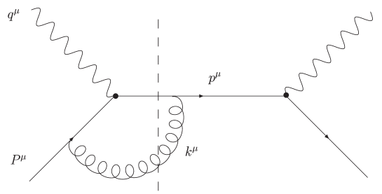
The calculation of the diagram in figure (7.1) involves the calculation of the trace:

$$2\frac{{\rm Tr}\left[(\hat{P}+m_{b})\gamma^{\mu}\hat{q}(1+\gamma_{5})(\hat{p}+\hat{k})\gamma^{\rho}\hat{p}\gamma_{\mu}\hat{q}(1+\gamma_{5})(\hat{P}-\hat{k}+m_{b})\gamma_{\rho}\right]}{(P\cdot k)(p\cdot k)},$$ (7.1)

where the operator $\hat{O}_{7}$ was inserted in the vertex, according to the equation (3.19).
The attribution of momenta is given in the figures.
Let us recall that the mass of the strange quark is neglected, so that $p^{2}=q^{2}=k^{2}=0$ and $P^{2}=m^{2}_{b}$.
The calculation of the trace is performed in dimensional regularization, in order to regularize infrared divergencies, in $n=4+\epsilon$ dimensions, with $\epsilon>0$.
The trace can be calculated according to the rules written in appendix (A): here $\hat{n}=\gamma^{\mu}n_{\mu}$.

Figure 7.2: Ladder diagram: square of the diagram describing the emission of the gluon from the initial quark.

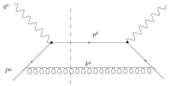
The ladder diagram in figure (7.2) produces the contribution

$$\frac{{\rm Tr}\left[(\hat{P}+m_{b})\gamma^{\rho}(\hat{P}-\hat{k}+m_{b})\gamma^{\mu}\hat{q}(1+\gamma_{5})\hat{p}\gamma_{\mu}\hat{q}(1+\gamma_{5})(\hat{P}-\hat{k}+m_{b})\gamma_{\rho}\right]}{(P\cdot k)^{2}}.$$ (7.2)

Figure 7.3: Interference diagram.

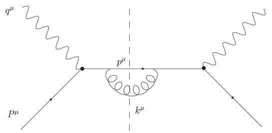
Finally the diagram (7.3) involves the trace

$$\frac{{\rm Tr}\left[(\hat{P}+m_{b})\gamma^{\mu}\hat{q}(1+\gamma_{5})(\hat{p}+\hat{k})\gamma^{\rho}\hat{p}\gamma_{\rho}(\hat{p}+\hat{k})\gamma^{\mu}\hat{q}(1+\gamma_{5})\right]}{(p\cdot k)^{2}}.$$ (7.3)

After the calculation of the traces we can insert the kinematics of section (4.2.1), by defining:

$$\omega = \frac{2E_{\gamma}}{m_{b}}$$

$$t = \frac{1-\cos\theta}{2}$$

$$y = \frac{2E_{s}}{m_{b}}.$$ (7.4)

The conservation of the quadrimomentum implies that

$$y=\frac{1-\omega}{1-\omega(1-t)},$$ (7.5)

so that the matrix element, to be integrated over the phase space, can be expressed in terms of just two variables, $\omega$ and $t$.
Summing the real diagrams the contribution to the matrix element in dimensional regularization turns out to be:

$$M(\omega,t) =$$

$$= -\frac{1}{\Gamma(1+\epsilon/2)}\frac{1}{4(1-\omega(1-t))^{3}(\epsilon+2)}\left[(1-t)^{\frac{\epsilon+2}{2}}(1-\omega)^{3}\left(\frac{1-\omega}{(1-\omega(1-t))}\right)^{\epsilon}\right.$$

$$\left(-8+8(1-t)\omega-4\omega^{2}(1+t)-4\epsilon(1-(1-t)\omega+\omega^{2}(1+t))-\epsilon^{2}\omega^{2}(1-t)\right)\left.\right]$$

The quantity of interest is (see equation (4.24))

$$\frac{1}{\Gamma_{0}}\frac{d\Gamma}{dx}=\frac{1}{2m_{b}}\frac{M(\omega,t)}{\omega^{1-\epsilon}t^{1-\epsilon/2}}d\Phi(\omega,t)\left[x-\omega^{2}t(1-t)\right].$$ (7.7)

$d\Phi(\omega,t)$ is the phase space described in appendix B.
The decomposition in (2.91) allows to underline terms giving rise to double logarithmic enhancement, (collinear or soft) logarithmic enhancement and finite terms.

$$A_{1} = \frac{1}{\Gamma(1+\epsilon/2)};$$ (7.8)

$$C_{1}(\omega) = \frac{\omega^{\epsilon}(\omega(\epsilon+2)-4)}{4\Gamma(1+\epsilon/2)};$$

$$S_{1}(t) = \frac{1-(1-t)^{1+\epsilon/2}}{\Gamma(1+\epsilon/2)};$$

$$F_{1}(\omega,t) = \frac{\omega t(2\omega^{2}t^{3}-\omega(\omega^{3}-2\omega^{2}+8\omega-6)t^{2})}{2(1-\omega(1-t))}+$$

$$+ \frac{\omega t(4\omega^{4}-10\omega^{3}+15\omega^{2}-13\omega^{2}+4)t-(1-\omega)^{2}(3\omega^{2}-2\omega+2))}{2(1-\omega(1-t))}.$$

The function $F_{1}$, since it does not give rise to infrared divergencies, can be calculated for $\epsilon\rightarrow 0$.
We are interested in the cumulative distribution, which takes from real emissions a contribution of the form:

$$D_{R}(x)=\int_{0}^{x}dx^{\prime}\int_{0}^{1}d\omega\int_{0}^{1}dt\ {1\over\Gamma_{0}}\ {d\Gamma\over dx^{\prime}}(\omega,t;\epsilon)\ \delta[x^{\prime}-\omega^{2}t(1-t)].$$ (7.9)

Figure 7.4: Region of the phase space to integrate: vertical axes $\rightarrow\omega$, horizontal axes $\rightarrow t$.

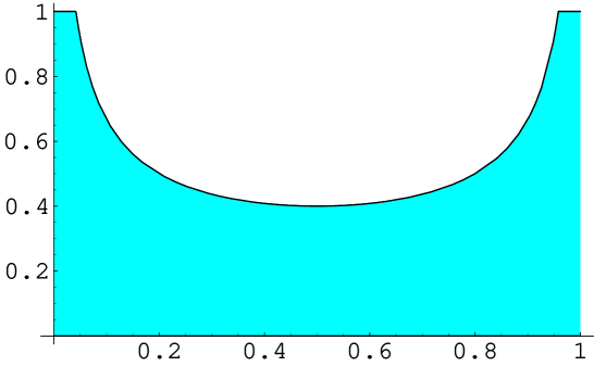
After the integration over the phase space we expect four kinds of terms:

• Poles in the regulator $\epsilon$: they parametrize the infrared singularities and cancel in the sum with virtual diagrams because the distribution we are dealing with is infrared-safe;

• Logarithmic terms diverging for $x\rightarrow 0$: with the matching procedure they are subtracted and inserted in the function $\Sigma(x;\alpha_{S})$;

• Constant terms: they enter the coefficient function $K(\alpha_{S})$;

• Remainder functions: terms that vanish in the limit $x\rightarrow 0$.

Figure 7.5: Whole phase space.

Figure 7.6: Complementary region.

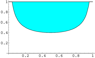
Integrating over $x^{\prime}$ we have:

$$D_{R}(x)=\int_{0}^{1}d\omega\int_{0}^{1}dt\ {1\over\Gamma_{0}}\ {d\Gamma\over dx^{\prime}}(\omega,t;\epsilon)\ \theta[x-\omega^{2}t(1-t)].$$ (7.10)

The remaining integrations are non-trivial because of the simultaneous presence of the kinematical constraint (see figure (7.4) and by the dimensional regularization parameter $\epsilon$. By using the identity

$$\theta[x-\omega^{2}t(1-t)]~{}=~{}1-\theta[\omega^{2}t(1-t)-x],$$ (7.11)

we separate these two effects and rewrite the distribution $D_{R}(x)$ as a difference between an integral over the whole phase space (fig. 7.6) and a integral over the complementary region (fig. 7.6):

$$D_{R}(x)=\int_{0}^{1}d\omega\int_{0}^{1}dt{1\over\Gamma_{0}}\ {d\Gamma\over dx}(\omega,t;\epsilon)\ -\ \int_{0}^{1}d\omega\int_{0}^{1}dt{1\over\Gamma_{0}}\ {d\Gamma\over dx}(\omega,t;0)\ \theta[\omega^{2}t(1-t)-x]~{}+~{}O(\epsilon).$$ (7.12)

In this way we have separated the two main sources of difficulty in the computation of equation (7.10).
The first integral must be evaluated for $\epsilon\neq 0$ because it contains poles in $\epsilon$, but is done over a very simple domain, independent of $x$: the integration can be performed without the introduction of special techniques with an advanced program of symbolic calculation. The result can be expanded in powers of $\epsilon$ and at this stage double and single poles in the regulator and constant arise.
The second integral does not contain any pole in $\epsilon$ and therefore one can take the limit $\epsilon\rightarrow 0$ in the integrand: it strongly depends on the kinematical constraint, which makes the analytical computation very complicated.
At first let us integrate over the variable $\omega$, since the analytical dependence on it in the constraint (4.24) seems to be simpler. The limits of integration are

$$\frac{\sqrt{x}}{\sqrt{t(1-t)}}<\omega<1.$$ (7.13)

Then, after the change of variable $y=\frac{1}{t}-1$, the integration can be performed over $y$, with the limits of integration

$$\tau<y<\frac{1}{\tau},$$ (7.14)

being

$$\tau=\frac{1-\sqrt{1-4x}}{1+\sqrt{1-4x}}.$$ (7.15)

The analytic integration is now very complicated and seems to resist to the attack of usual techniques: a powerful tool that can overcome this difficulty is the use of harmonic polylogarithms [75]. The general properties of this approach are outlined in appendix E.
The first step is the introduction of a proper basis of function: the one we singled out is

$$g[0;y] \equiv {1\over y}$$

$$g[-1;y] \equiv {1\over y+1}$$

$$g[-2;y] \equiv {1\over{\sqrt{y}(1+y)}}$$

$$g[-3;y] \equiv -{\sqrt{x}\over{2({1-\sqrt{x}\sqrt{y})}\sqrt{y}}}.$$ (7.16)

According to the theory described in appendix E, the harmonic polylogarithms (HPL) of weight 1 are defined as:

$$J[a;y] \equiv \int_{0}^{y}dy^{\prime}\ g(a;y^{\prime})\ \ \ \rm{for}\;a\neq 0$$

$$J[0;y] \equiv \log y.$$ (7.17)

In terms of usual functions, they read:

$$J[-1;y] \equiv \log(1+y)$$

$$J[-2;y] \equiv 2\arctan\sqrt{y}$$

$$J[-3;y] \equiv \log(1-\sqrt{x}\sqrt{y})$$ (7.18)

The HPL’s of weight 2 are defined for $(u,v)\not=(0,0)$ as

$$J[u,v;y]\equiv\int_{0}^{y}dy^{\prime}\ g[u;y^{\prime}]\int_{0}^{y^{\prime}}dy^{\prime\prime}g[v;y^{\prime\prime}]$$ (7.19)

and $J[0,0;y]=1/2\log^{2}y$. HPL’s of higher weight may be defined in an analogous way. They will not be used here.
The integration is not trivial: it is performed through chains of integration by parts of every terms, using the property

$$\frac{d}{dx}J(\vec{m}_{w};x)=g(a;x)J(\vec{m}_{w-1};x)$$ (7.20)

and algebraic manipulations. For example

$$\int\ y^{n}\ J(a,w;y)dy=\frac{y^{n+1}}{n+1}J(a,w;y)-\int\ \frac{y^{n+1}}{n+1}\ g(a;y)\ J(w;y)dy$$ (7.21)

The remaining integral can be simplified by using partial fractioning and following integrations by parts.
After this process every function appearing in the result is expressed in terms of algebraic functions or harmonic polylogarithms: in particular every transcendental function is expressed as a combination of hpl’s.
Once the undefined integral is calculated, one has to substitute the limits of equation 7.14 and the final result is, summing the two integrals:

$$D_{R}(x)=C_{F}{\alpha_{S}\over\pi}\ \left({m^{2}_{b}\over 4\pi\mu^{2}}\right)^{\epsilon/2}\ {1\over\Gamma(1+\epsilon/2)}\ \left[{2\over\epsilon^{2}}\ -{5\over 2\epsilon}\ -{1\over 4}\ \log^{2}x-\ {5\over 4}\ \log x+\ {1\over 4}\ +r_{1}(x)\right],$$ (7.22)

where $r_{1}(x)$ is a function vanishing for $x\rightarrow 0$.
From the matching procedure $r_{1}(x)$ can be recognized as the first term in the expansion of the remainder funtion (see section (7.3)) and turns out to be

$$r_{1}(\tau) =\frac{(\tau-1)(49\tau^{8}+468\tau^{7}+1797\tau^{6}+3642\tau^{5}+4450\tau^{4}+3642\tau^{3}+1797\tau^{2}+468\tau+49)}{12(\tau+1)^{5}(\tau^{2}+3\tau+1)^{2}}$$ (7.23)

$$+ \frac{-5-61\tau-317\tau^{2}-912\tau^{3}-1622\tau^{4}-1934\tau^{5}-1622\tau^{6}-912\tau^{7}-317\tau^{8}-61\tau^{9}-5\tau^{10}}{4(\tau+1)^{6}(\tau^{2}+3\tau+1)^{2}}\log\tau$$

$$- J[0,-3,\tau]+J[0,-3,1/\tau]-2J[0,-1,\tau]+J[-1,0,\tau]+J[-1,-3,\tau]-J[-1,-3,1/\tau]$$

$$- 2\sqrt{\tau}\arctan(\sqrt{\tau})\frac{(\tau+1)(2\tau^{2}+7\tau+2)}{(\tau^{2}+3\tau+1)^{2}}+\frac{\pi}{2}\sqrt{\tau}\frac{(\tau+1)(2\tau^{2}+7\tau+2)}{(\tau^{2}+3\tau+1)^{2}}+\frac{49}{12}$$

$$+ \frac{5}{4}\log\tau-\frac{5}{2}\log(\tau+1)+\log^{2}(\tau+1).$$

Let us notice that $\tau$ behaves as $x$ for small values of the transverse momentum

$$\tau(x)=x+O(x^{2})$$ (7.24)

and it is a unitary variable

$$\tau\rightarrow 0\ \ \ \rm{for} \ \ \ x\rightarrow 0$$ (7.25)

$$\tau\rightarrow 1\ \ \ \rm{for} \ \ \ x\rightarrow 1/4.$$ (7.26)

The relation (7.15) may be inverted as

$$x=\frac{\tau}{(\tau+1)^{2}}.$$ (7.28)

One can easily check that $r(\tau)$ vanishes for $\tau\sim x\rightarrow 0$, by using the properties

$$J[0,-1,0]=J[0,-3,0]=J[-1,0,0]=J[-1,-3,0]=0$$ (7.29)

$$\lim_{\tau\to 0}J[0,-3,1/\tau]=\lim_{\tau\to 0}J[-1,-3,1/\tau]=-\frac{\pi^{2}}{3}.$$ (7.30)

Finally let us observe that the extraction of the remainder function is based on a matching procedure: in order to avoid double counting we have subtracted the logarithmic terms already included in the resummation of logarithms, namely the equation (5.9) after the integration over $x$,

$$-\frac{\alpha_{S}A_{1}}{4}\log^{2}x+\alpha_{S}B_{1}\log x.$$ (7.31)

The constant appearing in (7.22) has to be summed to the virtual contribution to get the coefficient function.

7.2 Complete Calculation of Virtual Diagrams

Virtual corrections to $b\rightarrow s\gamma$ have been calculated in [57, 58] for a massive strange quark; we present here the computation in the massless case.
The diagrams consist of self-energy corrections to the heavy and light lines (see fig. (7.8) and (7.8)) and of vertex corrections to the operator $\hat{\mathcal{O}}_{7}$ (see figure (7.9)); we compute them in the $\overline{MS}$ scheme so as to be consistent with the (known) coefficient functions $C_{i}$. The computation can be done with standard Feynman parameter technique [16] or by a reduction using the integration by part identities [76].

Figure 7.7: Heavy quark self-energy diagram.

Figure 7.8: Light quark self-energy diagram.

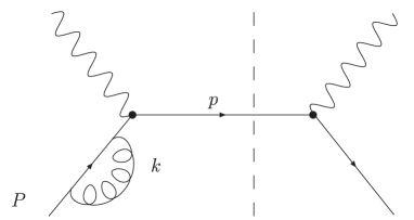
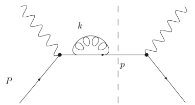
In order to show both techniques, let us start by calculating the self-energies with Feynman parameters. The diagrams are calculated in $n=4-\epsilon$ dimensions, to regularize ultraviolet divergencies, and off-shell to regularize infrared divergencies, $p^{2}\not=m^{2}$. The renormalization provide for the cancellation of ultraviolet divergencies by counterterms in a proper scheme, decided once for all. All the calculations can be consistent with the chosen renormalization scheme.
The calculation of the diagram in figure (7.8) gives

$$\Sigma=4\pi\alpha_{S}\mu^{\epsilon}\int\ \frac{d^{n}k}{(2\pi)^{n}}\ \frac{1}{k^{2}}\frac{1}{(P-k)^{2}-m_{b}^{2}}\left[\gamma^{\mu}(\hat{P}-\hat{k}+m_{b})\gamma_{\mu}\right]-(Z_{0}-1)m_{b}-(Z_{2}-1)\hat{p}.$$ (7.32)

$\mu$ is the renormalization scale.
The diagram can be written as

$$\Sigma=A(P^{2})+B(P^{2})\hat{P}$$ (7.33)

where $A(P^{2})$ and $B(P^{2})$ can be easily calculated, by introducing Feynman parameters as in appendix C. They turn out to be

$$A(P^{2}) = 4\pi\alpha_{S}\int\frac{dk^{\prime}}{(2\pi)^{n}}\int_{0}^{1}\frac{nm_{b}}{\left[k^{\prime 2}+(P^{2}-m^{2}_{b})x-P^{2}x^{2}\right]^{2}}-(Z_{0}-1)m_{b},$$

$$B(P^{2}) = 4\pi\alpha_{S}\int\frac{dk^{\prime}}{(2\pi)^{n}}\int_{0}^{1}\frac{(2-n)(1-x)}{\left[k^{\prime 2}+(P^{2}-m^{2}_{b})x-P^{2}x^{2}\right]^{2}}-(Z_{2}-1)m_{b}.$$ (7.34)

After a straightforward calculation one obtains the value of the counterterms which cancel the ultraviolet singularities of the diagram, in $\overline{MS}$ scheme they turn out to be

$$(Z_{0}-1) = \frac{\alpha_{S}}{\pi}\left[\frac{2}{\epsilon}-\gamma+\log 4\pi\right],$$

$$(Z_{2}-1) = \frac{\alpha_{S}}{\pi}\left[-\frac{1}{2\epsilon}+\frac{\gamma}{4}-\frac{1}{4}\log 4\pi\right].$$ (7.35)

Once the ultraviolet divergencies have been cancelled, the diagrams can be calculated on-shell and the infrared singularities can be regularized by taking $n=4+\epsilon$.
The contribution given by the diagram to the rate is

$$\Sigma_{1}=\frac{\partial A}{\partial P^{2}}|_{P^{2}=m^{2}_{b}}2m_{b}+B(m^{2}_{b})+2m^{2}_{b}\frac{\partial B}{\partial P^{2}}|_{P^{2}=m^{2}_{b}},$$ (7.36)

which reads

$$\Sigma_{1}=\frac{\alpha_{S}}{\pi}\left[\frac{1}{\epsilon}+\frac{\gamma}{2}+\frac{1}{2}\log\frac{m^{2}_{b}}{4\pi\mu^{2}}-1+\frac{1}{4}\log\frac{m^{2}_{b}}{\mu^{2}}\right].$$ (7.37)

For the massless self-energies in figure (7.8) the case is more involved. The only term contributing in $\Sigma_{1}$ is $B(0)$. We need to calculate just $B(p^{2})$ off-shell, subtract the ultraviolet divergencies with the counterterm and to determine $B(0)$, which reads

$$B(0)=\Sigma_{1}=\frac{\alpha_{S}}{\pi}\left[-\frac{1}{2\epsilon}-\frac{\gamma}{4}+\frac{1}{4}\log 4\pi\right].$$ (7.38)

Let us now briefly describe the evaluation of the vertex correction within the second method. One has to compute the scalar integral:

$$\mathcal{V}=\int{d^{n}k\over(2\pi)^{n}}\ {N(k^{2},P\cdot k,p\cdot k;\epsilon)\over k^{2}[(k-P)^{2}-m^{2}](k-p)^{2}},$$ (7.39)

where

$$N(k^{2},P\cdot k,p\cdot k;\epsilon)=32P\cdot k-32p\cdot k-16m^{2}_{b}+\mathcal{O}(\epsilon^{2})k^{2}+\mathcal{O}(\epsilon^{2})P\cdot kp\cdot k+\mathcal{O}(\epsilon^{2}){(p\cdot k)}^{2}.$$ (7.40)

$\mathcal{V}$ has at most a double pole in $\epsilon$ coming from the product of the soft and the collinear singularities. The terms in the numerator $N$, which vanish in the soft limit $k_{\mu}\rightarrow 0$, do not give rise to soft singularities and therefore produce at most a simple pole coming from the collinear or the ultraviolet region. Therefore the $\mathcal{O}(\epsilon^{2})$ terms in $N$ do not contribute in the limit $\epsilon\rightarrow 0$. Moreover, since the only terms in $N$ which can give ultraviolet divergencies are quadratic in $k$ and can produce at most a single pole in $\epsilon$, $\mathcal{V}$ can be safely calculated in $n=4+\epsilon$ dimensions to regularize just infrared divergencies.

Figure 7.9: Vertex correction diagram.

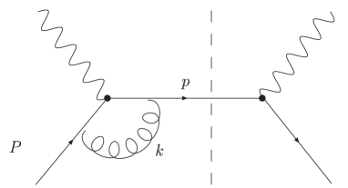
By expressing the scalar products in the numerator as linear combinations of the denominators as

$$k\cdot p = \frac{1}{2}\left(k^{2}-(k-p)^{2}\right),$$

$$k\cdot P = \frac{1}{2}\left(k^{2}-(k-P)^{2}+m_{b}^{2}\right),$$ (7.41)

we can reduce $\mathcal{V}$ to a superposition of scalar integrals of the form:

$${\rm T}[a,b,c]=\int{d^{n}k\over(2\pi)^{n}}\ {1\over[k^{2}]^{a}\ [(k-P)^{2}-m_{b}^{2}]^{b}\ [(k-p)^{2}]^{c}}$$ (7.42)

with $a,b,c\leq 1$. The above amplitudes can be related to each other by identities of the form [76]:

$$\int d^{n}k\ {\partial\over\partial k^{\mu}}\ {v^{\mu}\over[k^{2}]^{a}[(k-P)^{2}-m^{2}]^{b}[(k-p)^{2}]^{c}}=0$$ (7.43)

with $v^{\mu}=k^{\mu},p^{\mu},P^{\mu}$. By explicitly evaluating the derivatives and re-expressing the scalar products using eqs. (7.2), one obtains relations among amplitudes with shifted indices.

Figure 7.10: Massive tadpole diagram.

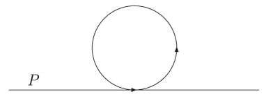
By solving the above identities, one can reduce all the amplitudes to the tadpole (figure 7.10), and obtains for the integral:

$$\mathcal{V}=\left(+{16\over\epsilon}-8+8\epsilon\right){1\over m^{2}_{b}}\ {\rm T}[0,1,0],$$ (7.44)

where

$${\rm T}[0,1,0]=C_{F}{\alpha_{S}\over 16\pi}\ \left({m^{2}\over 4\pi\mu^{2}}\right)^{\epsilon/2}\ {\Gamma(-\epsilon/2)\over 1+\epsilon/2}\ m_{b}^{2}.$$ (7.45)

The contribution associated to the vertex correction reads

$$\mathcal{V}=C_{F}\frac{\alpha_{S}}{\pi}\ \left({m^{2}\over 4\pi\mu^{2}}\right)^{\epsilon/2}\ \Gamma\left(1-\frac{\epsilon}{2}\right)\ \left[-\frac{2}{\epsilon^{2}}+\frac{2}{\epsilon}-2\right].$$ (7.46)

Summing self-energies and vertex corrections, and subtracting the $1/\epsilon$ poles according to the $\overline{MS}$ scheme, one obtains for their contribution to the rate $D_{V}$ :

$$D_{V}=C_{F}{\alpha_{S}\over\pi}\ \left({m^{2}_{b}\over 4\pi\mu^{2}}\right)^{\epsilon/2}\ \Gamma\left(1-{\epsilon\over 2}\right)\ \left[-{2\over\epsilon^{2}}+{5\over 2\epsilon}+4\log{m_{b}\over\mu_{b}}-3\right].$$ (7.47)

We have kept the factor in front of the square bracket unexpanded to simplify the computation of the total rate.
The virtual corrections to the remaining operators $\hat{\mathcal{O}}_{i\not=7}$ contain only (simple) ultraviolet poles in $\epsilon$, which are removed by renormalization; their contributions to $D_{V}$ amount only to finite constants and $\log m_{b}/\mu_{b}$.

7.3 Final Result: the Coefficient Function and the Remainder Function

Summing real and virtual contributions, the transverse momentum distribution for the decay $b\rightarrow s\gamma$ reads, to $O(\alpha_{S})$:

$$D(x)=1~{}+~{}C_{F}{\alpha_{S}\over\pi}\ \left[-{1\over 4}\ \log^{2}x-\ {5\over 4}\ \log x+\kappa_{1}+\ r_{1}(x)\right].$$ (7.48)

As expected, the result contains a double logarithm and a single logarithm of $x$, a finite term $\kappa_{1}$ and a function $r_{1}(x)$ vanishing in the limit $x\rightarrow 0$.
By expanding the resummed formula (2.127) to order $\alpha_{S}$ one obtains:

$$D(x) = \left(1+\frac{C_{F}\alpha_{S}}{\pi}\kappa_{1}\right)\left(1-\frac{A_{1}}{4}\alpha_{S}\log^{2}x+B_{1}\alpha_{S}\log x\right)+\frac{C_{F}\alpha_{S}}{\pi}r_{1}(x)$$

$$= 1-\frac{A_{1}}{4}\alpha_{S}\log^{2}x+B_{1}\alpha_{S}\log x+\frac{C_{F}\alpha_{S}}{\pi}\kappa_{1}+\frac{C_{F}\alpha_{S}}{\pi}r_{1}(x)+O(\alpha_{S}^{2}).$$

The matching procedure consists in the identification of the values of $\kappa_{1}$ and $r_{1}(x)$ and the computation allows to we check the values for $A_{1}$ and $B_{1}$, evaluated in [1] using general properties of QCD radiation.
The value of the first term in the expansion of the coefficient function is

$$k_{1}=-\ {11\over 4}-\ {\pi^{2}\over 12}+~{}4\log{m_{b}\over\mu},$$ (7.50)

The value of the first term in the expansion of the remainder function is given in equation (7.23).
As explained in previous sections, the remaining operators $\hat{\mathcal{O}}_{i\not=7}$ contribute to $D(x)$ only by finite terms $\tilde{r}_{i}$ and remainder functions. Since the constants $\tilde{r}_{i}$ come from virtual diagrams alone, we can quote their result from [57, 58] and present an improved formula for the coefficient function, in analogy with [77]:

$$K(\alpha_{S})~{}=~{}1+{\alpha_{S}\over 2\pi}\sum_{i=1}^{8}{C^{(0)}_{i}(\mu_{b})\over C^{(0)}_{7}(\mu_{b})}\left(\Re\ \tilde{r}_{i}+\gamma^{(0)}_{i7}\log{m_{b}\over\mu_{b}}\right)+{\alpha_{S}\over 2\pi}{C^{(1)}_{7}(\mu_{b})\over C^{(0)}_{7}(\mu_{b})}+\mathcal{O}(\alpha_{S}^{2})$$ (7.51)

where

$$\tilde{r}_{i} = r_{i}~{}~{}~{}~{}~{}i\not=7$$

$$\tilde{r}_{7} = \frac{8}{3}\left(f-4\log\frac{m_{b}}{\mu_{b}}\right)=-\frac{22}{3}-\frac{2\pi^{2}}{9}.$$ (7.52)

Let us remark that only the coefficients related to the operators with $i=1,2,7,8$ are relevant, because the others are multiplied by very small coefficient functions and can be neglected:

$$r_{1} = -{1\over 6}r_{2}$$

$$\Re\ r_{2} = -4.092-12.78(0.29-m_{c}/m_{b})$$

$$r_{8} = {4\over 27}(33-2\pi^{2}).$$ (7.53)

The analytic expressions for the coefficient functions as well as a standard numerical evaluation are given in [52]. The anomalous dimension $\gamma^{(0)}_{77}$ is derived from the coefficient of the logarithmic term in $k_{1}$. The values of $\gamma_{i7}^{(0)}$ are [52]:

$$\gamma^{(0)}_{i7}=\left(-{208\over 243},{416\over 81},-{176\over 81},-{152\over 243},-{6272\over 81},{4624\over 243},{32\over 3},-{32\over 9}\right).$$ (7.54)

The calculation of the coefficient function in (7.51) complete the program of next-to-leading resummation.
The remainder function is in general negligible for small transverse momenta, for larger value of transverse momenta a small change in the fixed order prediction can be noticed, as shown in figure (7.11). The figure shows that for larger values than $x=0.1$ the remainder function produces a correction of the order of $O(10-15\%)$ with respect to the only logarithmic contribution.
Obviously this happen where logarithms are already quite small and this effect can be taken into account near the fully inclusive region of the spectrum, but can be discarded in the semi-inclusive one (small $p_{t}$).

Figure 7.11: Comparison between the full fixed order calculation for $D(x)$ (solid line) and the logarithmic approximation (dashed line).

Chapter 8 Mass Effects from the Final Quark

8.1 Motivations

In this chapter preliminary results are shown, concerning the structure of infrared logarithms in heavy flavour decays, where both the decaying quark and the final quark are massive.
Example of these transitions are $top\rightarrow beauty$, $beauty\rightarrow charm$, $beauty\rightarrow strange$ (with a massive strange quark).
The main phenomenological difference with respect to transitions like $beauty\rightarrow up$ or $beauty\rightarrow strange$ (if we neglect the strange quark mass) is that in this case the hadronic final jet branches from a massive quark.
In order to be plain, we deal with a specific physical distribution, the photon spectrum distribution in $b\rightarrow s\gamma$, but it should be clear that the results apply to other $Q\rightarrow Q$ transitions with few changes in kinematics.
In particular from a phenomenological point of view it should be very interesting to apply these results to the transition

$$b\rightarrow c.$$

In fact it has a much higher rate than the rare process we are considering and it is widely investigated from an experimental point of view. However, being the kinematics more complicated, we decided to start from a simpler process, anyhow having a great phenomenological importance.
In this chapter we analyze the main differences with respect to the massless case, due to soft gluon emissions, which are affected by the the presence of a mass in the final state.

8.2 Kinematics

Let us consider the photon spectrum in the decay

$$B\rightarrow X_{s}+\gamma$$ (8.1)

where $X_{S}$ is an hadronic jet containing a strange quark.
At the tree level in the partonic process it is

$$b\rightarrow s\gamma.$$ (8.2)

Two practical reasons drove us to consider this specific process: first of all at the tree level it is a two body decay and its kinematics is very simple, moreover the results for this decay neglecting the strange quark mass are well known and it can be interesting to compare the effects due to the presence of the mass. When we will need such a comparison, the case with the strange mass neglected will be referred as the massless case.
At the tree level the photon energy is fixed by kinematics

$$E_{\gamma}={m^{2}_{b}-m^{2}_{s}\over 2m_{b}}.$$ (8.3)

In the following calculations $m_{s}\not=0$, but

$$\mu={m_{s}^{2}\over m^{2}_{b}}\ll 1$$

Radiative corrections are given by gluon emissions

$$b\rightarrow s\gamma g_{1}\dots g_{n}$$ (8.4)

which spread and shift the photon spectrum peak.
Let us define the invariant jet mass

$$M^{2}_{X}=(\sum_{i}p_{i})^{2}$$

where $p_{i}$ are parton (strange quark + gluons) momenta.
The photon energy is related to the invariant mass by the relation

$$E_{\gamma}={m_{b}^{2}-M^{2}_{X}\over 2m_{b}}.$$ (8.5)

Let us define a unitary variable $X_{\gamma}$ as

$$X_{\gamma}=E_{\gamma}\ {2m_{b}\over m^{2}_{b}-m^{2}_{s}}$$ (8.6)

so that $X_{\gamma}\rightarrow 1$ is the elastic limit.
Another useful relation is

$$(1-X_{\gamma})={m^{2}_{X}\over m^{2}_{b}-m^{2}_{s}}$$ (8.7)

where

$$m^{2}_{X}=M^{2}_{X}-m^{2}_{s}.$$ (8.8)

If $m_{s}=0$

$$(1-X_{\gamma})={m^{2}_{x}\over m_{b}^{2}}={M^{2}_{X}\over m^{2}_{b}}$$

and we can recognize the kinematics of the massless case.
The correct hard scale in the process of jet evolution is

$$Q=2E_{X}$$ (8.9)

as discussed in [78]. $E_{X}$ is the energy of the hadronic jet and the factor 2 is introduced to simplify the calculations.
The jet energy is related to the invariant mass by the relation

$$E_{X}={m^{2}_{b}+M^{2}_{X}\over 2m_{b}}$$ (8.10)

Because of (8.5) $M^{2}_{X}$-distribution and photon spectrum are strictly related: in the following we will calculate relations for the $M^{2}_{X}$-spectrum because it involves just the evolution of the jet, and then we will go back again to the photon spectrum using (8.5).

8.3 One Soft Gluon Emission

Let us now consider $\alpha_{S}$ corrections and in particular one soft real gluon emission

$$b\rightarrow s\gamma g.$$ (8.11)

Let us define

$$p^{\mu}_{X}=p^{\mu}_{s}+p^{\mu}_{g}$$ (8.12)

so that $p^{2}_{X}=M^{2}_{X}$.
It is well known that the rate for one real gluon emission is affected by infrared singularities of soft and collinear nature, which are cancelled by virtual emissions, for infrared-safe variables.
Here we are focused on the eikonal approximation, described in section (2.10). As it was discussed there, this approximation allows to study the structure of logarithms arising from soft gluon emissions and it lies on the definition of an eikonal current

$$J^{\mu}=g_{S}T_{b}{p^{\mu}\over p_{b}\cdot p_{g}}-g_{S}T_{s}{p^{\mu}\over p_{s}\cdot p_{g}}$$ (8.13)

where $p^{\mu}_{b}$ is the beauty quark momentum and $T_{i}$ are color generators.
The squared matrix element is given by

$$-g_{\mu\nu}J^{\mu}J^{\nu} = 4\pi\alpha_{S}\left(2T_{b}\cdot T_{s}{p_{b}\cdot p_{s}\over(p_{b}\cdot p_{g})(p_{s}\cdot p_{g})}-T^{2}_{b}{m^{2}_{b}\over(p_{b}\cdot p_{g})^{2}}-T^{2}_{s}{m^{2}_{s}\over(p_{s}\cdot p_{g})^{2}}\right)$$ (8.14)

$$= {\cal{M}}_{bs}+{\cal{M}}_{bb}+{\cal{M}}_{ss}$$

The difference with respect to the massless case is that we need to calculate all the three terms in the previous formula, in particular the third one is different from zero in this case: moreover the different kinematics produces corrections to the other terms.
The color structure is trivial because of the presence of just two coloured partons in the hard vertex.
The hard vertex conserves the color, so that

$$T_{b}=T_{s}$$

which implies

$$T^{2}_{b}=T^{2}_{s}=T_{b}\cdot T_{s}=C_{F}.$$

Because of the relation (8.5) we can calculate the invariant mass distribution to get the photon spectrum: the kinematical constraint can be derived by (8.12) whose square is

$$m^{2}_{s}=M^{2}_{X}-2p_{X}\cdot p_{g}=M^{2}_{X}-2E_{g}E_{X}\left(1-\sqrt{1-{4M^{2}_{X}\over Q^{2}}}\cos\theta\right)$$ (8.15)

where $\theta$ is the angle between the strange quark and the gluon.
Let us now define

$$\omega={2E_{g}\over Q}={E_{g}\over E_{X}}$$ (8.16)

$$z=\cos\theta$$ (8.17)

the constraint becomes

$${1\over Q^{2}}\ \delta\left[{m^{2}_{X}\over Q^{2}}-{1\over 2}\omega\left(1-\sqrt{1-{4M^{2}_{X}\over Q^{2}}}z\right)\right].$$ (8.18)

Now we have to integrate the squared matrix element over the phase space with the kinematical constraint

$$\frac{1}{\Gamma_{0}}\left.\frac{d\Gamma}{dM^{2}_{X}}\right)_{SOFT}=\int{d^{3}p_{g}\over(2\pi)^{3}2E_{g}}\left(-g_{\mu\nu}J^{\mu}J^{\nu}\right){1\over Q^{2}}\delta\left[{m^{2}_{X}\over Q^{2}}-{1\over 2}\omega\left(1-\sqrt{1-\frac{4M^{2}_{X}}{Q^{2}}}\ z\right)\right].$$ (8.19)

The kinematical constraint does not introduce particular changes in the limits of integration of the phase space, which turn out to be

$$0< \omega <1,$$

$$-1< z <1.$$ (8.20)

Let us consider the three terms in the eikonal current separately: the dominant contribution, the one giving the leading logs in the massless case, is

$${\cal{M}}_{bs}=8\pi\alpha_{S}\ \left({p_{b}\cdot p_{s}\over(p_{b}\cdot p_{g})(p_{s}\cdot p_{g})}\right).$$ (8.21)

The integrations gives

$${1\over\Gamma_{0}}\left.{d\Gamma\over dM^{2}_{X}}\right)_{bs}=\alpha_{S}{C_{F}\over\pi}\ {1\over m^{2}_{X}}\ {E_{X}\over p_{X}}\log\left[{E_{X}+p_{X}\over E_{X}-p_{X}}\right]$$ (8.22)

where $p_{X}=\sqrt{E^{2}_{X}-M^{2}_{X}}$.
Recalling that

$$M^{2}_{X} = m^{2}_{b}(\mu+(1-\mu)(1-X_{\gamma}))$$ (8.23)

$$\approx m^{2}_{b}(\mu+(1-X_{\gamma}))$$

we have

$$\frac{1}{\Gamma_{0}}\left.\frac{d\Gamma}{dM^{2}_{X}}\right)_{bs}={1\over m^{2}_{b}-m^{2}_{s}}\ \alpha_{S}{C_{F}\over\pi}{1\over 1-X_{\gamma}}\log\left[\mu+(1-X_{\gamma})\right]$$ (8.24)

up to terms with no logarithmic enhancement.
The argument of the logarithm signals that the most interesting feature in this case is the interplay between the variable $(1-X_{\gamma})$ and the parameter $\mu$; in fact we can clearly discriminate three different regimes:

• if $(1-X_{\gamma})\gg\mu$ we fall in the massless case, getting the usual double logarithmic structure

  $$\log[1-X_{\gamma}]\over 1-X_{\gamma};$$

• if $(1-X_{\gamma})\ll\mu$, that is very near the endpoint we have a quasi-collinear logarithm

  $$\log[\mu]\over 1-X_{\gamma}.$$

  The collinear enhancement disappears because of the mass screen from the massive final parton: in this case we have a single log structure;

• if $(1-X_{\gamma})\sim\mu$ both the terms contribute and we have an interplay between the massless and massive case.

Figure 8.1: The figure shows the different regime discussed above in the double logarithmic approximation. The red line represents the full result obtained in (8.24), compared with the massless case (green line) and with purely massive case (blue line). The picture graphically shows the behaviours and the approximations discussed in the section: far from the endpoint the mass is negligible and the massless result is reproduced; approaching the endpoint the mass effect makes its appearance.

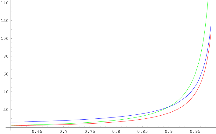
The second contribution to the current that we want to calculate is

$${\cal{M}}_{bb}=-4\pi\alpha_{S}{m^{2}_{b}\over(p_{b}\cdot p_{g})^{2}}.$$ (8.25)

After the integration we get

$${1\over\Gamma_{0}}\left.{d\Gamma\over dM^{2}_{X}}\right)_{bb}=-\alpha_{S}{C_{F}\over\pi}{1\over m^{2}_{X}}.$$ (8.26)

Recalling (8.7)

$${1\over\Gamma_{0}}\left.{d\Gamma\over dM^{2}_{X}}\right)_{bb}=-\alpha_{S}{C_{F}\over\pi}{1\over m^{2}_{b}-m^{2}_{s}}{1\over 1-X_{\gamma}}$$ (8.27)

This result represents the usual soft contribution as expected from the massless case: this is the only term not affected by the presence of a massive quark in the final state.
The last term in the current is new with respect to the massless case, because it doesn’t appear if $m_{s}=0$

$${\cal{M}}_{ss}=-4\pi\alpha_{S}{m^{2}_{s}\over(p_{s}\cdot p_{g})^{2}}.$$ (8.28)

The integration gives

$${1\over\Gamma_{0}}{d\Gamma\over dM^{2}_{X}}\left.\right)_{bb} = \alpha_{S}{C_{F}\over\pi}{m^{2}_{X}\over M^{2}_{x}m^{2}_{s}}=$$ (8.29)

$$= \alpha_{S}{C_{F}\over\pi}{1\over m_{b}^{2}-m^{2}_{s}}\left[\ {1\over 1-X_{\gamma}}-{1\over 1-X_{\gamma}+\mu}\ \right].$$

Let us note that (8.29) is zero if $m_{s}=0$ as we expected from the current.
The result shows a pure soft term, $1\over 1-X_{\gamma}$, and a term screened by the massive quark, $1\over(1-X_{\gamma})+\mu$: for $(1-X_{\gamma})\ll\mu$ the second term is no longer enhanced and we can neglect it.
The photon spectrum for soft emissions becomes

$${1\over\Gamma_{0}}{d\Gamma\over dX_{\gamma}}\left.\right)_{soft} = \delta(1-X_{\gamma})-\alpha_{S}A_{1}{1\over 1-X_{\gamma}}\log\left[{1\over(1-X_{\gamma})+\mu}\right]$$ (8.30)

$$- \alpha_{S}\ 2S_{1}\ {1\over 1-X_{\gamma}}+\alpha_{S}\ S_{1}\ {1\over(1-X_{\gamma})+\mu}$$

Let us note that for $m^{2}_{s}\rightarrow 0$ we get the massless result, while for $\mu\gg(1-X_{\gamma})$ the soft logarithm has a coefficient twice with respect to the massless case.
We defined

$$A_{1}={C_{F}\over\pi},$$ (8.31)

$$S_{1}=-{C_{F}\over\pi},$$ (8.32)

in analogy with the massless case.

8.4 Quasi-Collinear Emissions

The mass of the quark in the final state provides a natural cut-off for real collinear emissions: gluon emissions have to respect an angular restriction, known as dead cone effect, as discussed in section (2.10).
In this case we can tell two main behaviours: if the mass of the final quark is comparable to the hard scale (as maybe it could be for the transition $b\rightarrow c$) then the collinear logarithmic enhancement, matter of fact, disappears. In fact logarithmic terms will surely appear as in every case where different energy scales are involved, but these logarithms can be considered small, or to be more precise, not enhanced, because the two scales are not very much different.
Otherwise, if the final quark mass does not vanish, but is small with respect to the hard scales, collinear logarithms turn into less divergent terms, which we will call quasi-collinear.
The formal difference is that in this case the collinear logarithms does not diverge when the variable we are considering (for example $E_{\gamma}$) reaches the endpoint of the spectrum; from a physical point of view this means that the collinear emission is screened because of the dead cone effect.
The emission is still described by the Altarelli-Parisi kernel (2.68),

$$P_{qq}(\omega)=\frac{2-2\omega+\omega^{2}}{\omega}\stackrel{{\scriptstyle{\rm leading}}}{{\rightarrow}}\frac{2}{\omega},$$ (8.33)

but the integration over the polar angle is restricted according to the relation (2.105):

$$z>1-\frac{M^{2}_{X}}{Q^{2}}.$$ (8.34)

The integration over the phase space gives the result in (8.24) which represents the leading logarithmic approximation and therefore has both collinear and soft enhancement.
As stated above, while in the massless case the distribution formally diverges as

$$\frac{\log(1-X_{\gamma})}{1-X_{\gamma}}$$ (8.35)

at the endpoint of the spectrum, in this case the divergence is less dramatic and goes as

$$\frac{\log\mu}{1-X_{\gamma}}.$$ (8.36)

As discussed above if the mass of the initial and final quark are not much different, that is their masses does not different for one or more scales of magnitude, then this enhancement is no longer present: physically this means that if the masses are similar the collinear emission is so inhibited to be unrelevant.

8.5 Final Considerations

When the mass of the final quark is considered a new parameter is introduced in the calculation and this makes the structure of the result richer even at the logarithmic level. Obviously we expect that a complete calculation would show an increasing number of regular functions, with respect to the massless case, depending on the kinematics and in particular from the ratio of the masses of the quarks.
Concerning the logarithmic structure, which we are interested in, the introduction of the mass of the final quark introduces different regimes, which mainly depend on the value of this mass.
For real emissions we have studied the behaviour of the eikonal current, showing that if the mass is negligible the result of the massless case are obtained: however, studying a specific case, for example the photon spectrum, it is shown that near the endpoint the presence of the mass changes the spectrum giving a less divergent behaviour, because the logarithm of collinear nature is screened. In fact, due to the presence of the mass, the collinear emission under a minimum angle is forbidden (dead cone effect).
Moreover the mass introduces new terms in the eikonal current (which correctly disappear in the massless limit). The importance of each term strongly depend on the value of the mass: if the mass is small the effect is a correction to the massless case, if the mass is large the structure changes sizeably. In this case (see eq. (8.30)), for example, the double logarithmic enhancement disappears, the soft contribution has a coefficient twice the one of the massless case and the collinear emission can be neglected at this level of accuracy.
The results discussed in the previous sections are only preliminary: they should be developed to study the resummation of large logarithms when they appear and they should apply to different phenomenologies to understand when the effects of the final mass can be relevant.
In fact the presence of the mass manifest itself, as discussed, in different point of the spectrum: if the mass is small just at the endpoint, if the mass is large in regions far from the endpoint. If they manifest very near the endpoint it is very probable that they are overwhelmed by non perturbative effects and will be difficult to study and show. This implies that the application of this formalism should show different behaviours in the cases of the transition $b\rightarrow c$ (where the final mass is large) and in $b\rightarrow s\gamma$ (where the final mass is reasonably small).
We expect that the calculation of virtual diagrams will have the main effect to introduce plus distribution, for example

$$\frac{1}{1-X_{\gamma}}\rightarrow\frac{1}{(1-X_{\gamma})}_{+}$$ (8.37)

without changing the general structure of the result.

Chapter 9 Conclusions

The main topic of our work has been the calculation of the transverse momentum distribution of the $strange$ quark with respect to the photon direction, in the rare decay of the $beauty$ quark $b\rightarrow s\gamma$.
The physical motivations which lead us to study this particular process are outlined in chapter 4: there a discussion of the physical effects which lead to a generation of transverse momentum are described. In particular we focused our attention on the perturbative part, whose limits give informations about the structure of non perturbative contributions: such a distribution is a typical case where large logarithms appear near the border of the phase space, for the emission of soft and collinear gluons.
The appearance of logarithms always occurs in calculations where different scales are involved: however if the scales have very different sizes these logarithms becomes so large to spoil the perturbative expansion.
In the past years a technique to resum them was developed, in order to obtain an improved perturbative formula, with a range of applicability in a wider region of the phase space: this technique was successfully applied to processes at high energies, namely of the order of intermediate boson mass. Our aim was an application of such a technique to processes at lower energies, in our case at the energy of the $beauty$ quark mass.
In this case theoretical predictions are quite involved even in inclusive quantities: several poorly known parameters appear, such as CKM matrix elements or the quark mass, so that a stringent check of QCD at this scale of energies is not trivial. Matter of fact there are not indications that QCD should fail at this scale of energies nor a very precise check of its reliability.
The strong coupling constant seems to be small enough to allow a reliable perturbative expansions, and in distributions such as the one we studied the technique of resummation seems to be necessary and viable. However only a precise calculation, for example with next-to-leading accuracy, as we performed, compared with equally precise experimental data can suggest if the perturbative QCD is reliable or other effects play a crucial role.
This thesis is divided in a first part, where general tools to deal with QCD corrections in $b$ physics are outlined and a second part where the calculations we have performed are explicitely described.
After a description of the kinematical properties of the process of interest (Chapter 4), in Chapter 5 the resummation of large logarithms, performed with the purposes indicated above, is shown.
As usual even the resummed formula cannot be applied in the whole phase space, since near the infrared region non perturbative effects make their appearance and singularities appear in the resummed formula. These singularities give information about the non perturbative physics.
In Chapter 6 the comparison with a complementary distribution calculated for the same process, the threshold distribution, is outlined: the comparison with the different structure of singularities allows to conclude that in the transverse momentum case the non perturbative effects, above all the Fermi Motion, cannot be dealt with as in the threshold case. There a new non perturbative function (shape function), based on the HQET was introduced, here this approach is not viable, for the motivations contained in Chapter 6. The main reason is that in the threshold case Fermi Motion effects and hadronization can be separated by a scale, while in the transverse momentum case this does not occur. One should try in the latter case an alternative approach, possibly based on a different effective theory, as outlined in the text.
Finally the calculation is completed in Chapter 7, where a complete computation of real and virtual diagrams to order $\alpha_{S}$ is performed: this is necessary to extract some ingredients appearing in the general resummed formula, above all the constants involved in the coefficient function. Moreover it allows the extraction of the remainder function, the regular function describing the behaviour of the distribution in the hard region of the phase space: its knowledge is not strictly required for a next-to-leading resummation, but can improved the quality of the prediction far from the semi-inclusive region. However most of the events are expected in the region of small transverse momenta and therefore the phenomenological impact of the remainder function is expected to be of a few percent.
On the other side, the analytical computation of this term, which could seem academical, is an interesting application of techniques of advanced analytical calculation, as described in Chapter 7, which can be used for future purposes to approach the computation of other processes.
In the last Chapter, 8, a different topic is sketched: the effect of the mass of the final quark in $b$ decays. The result there presented are preliminary, since a resummation of the logarithms has not been performed yet and only the logarithmic structure to one loop is analyzed. However this is the first step towards a more general approach, taking into account the logarithmic enhancement in decays with a massive final quark. This will have an important application for the transition $b\rightarrow c$, where the mass of the $charm$ quark cannot be surely neglected. This process is very interesting from a phenomenological point of view: having a large rate, its study is intense at the $b$-factories.
To summarize, the main object of our work has been the application of the logarithmic resummation to the decay of an heavy quark. The calculation has been performed for the first time with next-to-leading accuracy, including constants and remainder terms, and the comparison with experimental data could be very useful to verify informations about the reliability of perturbative QCD in $b$ decays, the role played by non perturbative physics.
As underlined during the text, the process of interest is a rare decay, but it can be considered as a first step to face other processes that are very interesting from the phenomenological point of view.
This work could have several and possibly interesting extensions: first of all we hope that a systematic phenomenological study could be carried on within an extended comparison with data collected at the $b$ factories. Obviously this would be crucial to argue the correctness of the approaches that are used in $b$ decays, such as perturbative QCD.
A second point would be the extension of the shape function approach to the $p_{t}$ case: as underlined during the text, physical reasons forbid the application of this approach to the $p_{t}$ case and one should try to use different tools. Let us notice here that a good parametrization of non perturbative effects is crucial, not only for this particular decay, but also for other important decays, such as $b\rightarrow u$, because the same non perturbative functions are involved.
A further point would be the application of these techniques to other $b$ quark decays and to other distributions, for example the jet broadening, in order to reach a more complete knowledge of the dynamics of QCD at this scale of energies.
Finally the results of Chapter 8 should be completed to face more general problems, such as the decay of a $beauty$ quark into another massive quark, mainly a $charm$, but also a $strange$. The study of mass effects in perturbative calculation and in the resummation of logarithms can give higher reliability of the predictions of the theory.

Part III Appendices and Bibliography

Appendix A Feynman Rules and Numerator Algebra

This appendix contains relevant Feynman rules, used in the calculations performed in perturbative QCD. Feynman rules are extracted by the lagrangian of the theory, which reads:

$${\cal{L}}_{QCD} = \overline{\Psi}(i\gamma^{\mu}\partial_{\mu}-m)\Psi-\frac{1}{4}(\partial_{\mu}A^{a}_{\nu}-\partial_{\nu}A^{a}_{\nu})^{2}+g_{S}A^{a}_{\mu}\overline{\Psi}\gamma^{\mu}t^{a}\Psi$$ (A.1)

$$- gf^{abc}(\partial_{\mu}A^{a}_{\nu})^{2}A^{b\mu}A^{c\nu}-\frac{1}{4}(f^{eab}A^{a}_{\mu}A^{b}_{\nu})(f^{ecd}A^{b\mu}A^{d\nu}).$$

Ingoing quark:

$$=u(p,s)\ {\rm(for\ quark)},\overline{v}(p,s)\ {\rm(for\ antiquark)}$$ (A.2)

Outgoing quark:

$$=\overline{u}(p,s)\ {\rm(for\ quark)},v(p,s)\ {\rm(for\ antiquark)}$$ (A.3)

Ingoing gluon:

$$=\epsilon(k,\lambda)$$ (A.4)

Outgoing gluon:

$$\epsilon^{\ast}(k,\lambda)$$ (A.5)

Quark propagator:

$$=i\frac{\gamma^{\mu}p_{\mu}-m}{p^{2}-m^{2}+i\epsilon}$$ (A.6)

Gluon propagator:

$$=-i\delta_{\alpha\beta}\left[\frac{g_{\mu\nu}+\eta\frac{k_{\mu}k_{\nu}}{k^{2}}}{k^{2}+i\epsilon}\right]$$ (A.7)

Quark-Gluon vertex:

$$=-ig_{S}\gamma^{\mu}t^{a}_{ij}$$ (A.8)

3-gluon vertex:

$$= - g_{S}f^{abc}\left[g^{\mu\nu}(k-p)^{\rho}+g^{\nu\rho}(p-q)^{\mu}+\right.$$ (A.9)

$$+ g^{\rho\mu}(q-k)^{\nu}]$$

4-gluon vertex:

$$= - ig_{S}[f^{abe}f^{cde}(g^{\mu\rho}g^{\nu\sigma}-g^{\mu\sigma}g^{\nu\rho})$$

$$+ f^{ace}f^{bde}(g^{\mu\nu}g^{\rho\sigma}-g^{\mu\sigma}g^{\nu\rho})$$

$$+ f^{ade}f^{bce}(g^{\mu\nu}g^{\rho\sigma}-g^{\mu\rho}g^{\nu\sigma}]$$

Ghost vertices and propagator are not important for our work and will not be recalled.
The factor $\eta$ in the gluon propagator selects the gauge: all the calculation have been performed in the Feynman gauge which corresponds to $\eta=0$.
Sum over polarizations:

$$\sum_{s}u(p,s)\overline{u}(p,s)=\gamma^{\mu}p_{\mu}+m,$$ (A.11)

$$\sum_{s}v(p,s)\overline{v}(p,s)=\gamma^{\mu}p_{\mu}-m.$$ (A.12)

In the Feynman gauge the sum over the polarizations of external gluons allows the following replacement

$$\sum_{\lambda}\epsilon^{\ast}_{\mu}(\lambda)\epsilon_{\nu}(\lambda)\rightarrow-g_{\mu\nu}.$$ (A.13)

In the calculation of matrix elements in dimensional regularization traces of gamma matrices arise. The following properties have been used (n = dimension of the space-time):

$$\{\gamma^{\mu},\gamma^{\nu}\} = 2g^{\mu\nu}$$

$$\gamma^{\mu}\gamma_{\mu} = n$$

$${\rm Tr}(\gamma^{\mu}\gamma^{\nu}) = 4g^{\mu\nu}$$

$$\gamma^{\mu}\gamma^{\nu}\gamma_{\mu} = (2-n)\gamma^{\nu}$$

$$\gamma^{\mu}\gamma^{\nu}\gamma^{\rho}\gamma_{\mu} = 4g^{\nu\rho}+(n-4)\gamma^{\nu}\gamma^{\rho}.$$ (A.14)

In $n$ dimension one can consistently introduce a matrix $\gamma_{5}$ in a scheme where the property

$$\{\gamma_{g},\gamma_{\mu}\}=0$$ (A.15)

holds. $\gamma_{5}$ in 4 dimension reads:

$$\gamma_{5}=i\gamma_{0}\gamma_{1}\gamma_{2}\gamma_{3}.$$ (A.16)

Traces of an even number of gamma matrices and a $\gamma_{5}$ vanish:

$${\rm Tr}[\gamma_{5}\gamma_{\mu_{1}}\dots\gamma_{\mu_{2n}}]=0.$$ (A.17)

The metric chosen to perform the calculations is

$$g_{\mu\nu}=\left(\begin{array}[]{cccc}1&0&0&0\\ 0&-1&0&0\\ 0&0&-1&0\\ 0&0&0&-1\end{array}\right).$$ (A.18)

Appendix B Phase Space in Dimensional Regularization

The formula used to calculate the decay rate of a particle in its rest frame is

$$d\Gamma=\frac{1}{2m}\ d\Phi_{n}\ \delta(\sum_{i}p_{i}^{\mu})\ |\overline{M}|^{2}.$$ (B.1)

$m$ is the mass of the particle, $\Phi_{n}$ is the $n$-body phase space, $\delta(\sum_{i}p_{i}^{\mu})$ assures the momentum conservation and $|\overline{M}|^{2}$ is the squared matrix element of the process.
For the distribution of the transverse momentum in $b\rightarrow s\gamma$, $|\overline{M}|^{2}$ has been calculated in Chapter 7 , in this appendix the results for the 2-body and 3-body phase space in dimensional regularization are shown: these terms appears in the calculations of the Born amplitude and in radiative corrections.
The lowest order process is $b\rightarrow s\gamma$.
The general expression for the phase space is

$$d\Phi_{2}=\frac{d^{n}p}{(2\pi)^{n}}\frac{d^{n}q}{(2\pi)^{n}}(2\pi)\delta_{+}(p^{2})(2\pi)\delta_{+}(q^{2})(2\pi)^{n}\delta(P^{\mu}-p^{\mu}-q^{\mu}),$$ (B.2)

where $p^{\mu}$ is the strange quark momentum, $q^{\mu}$ the photon momentum and $P^{\mu}$ the $beauty$ quark momentum and

$$\delta_{+}(p^{2})=\delta(p^{2})\theta(p^{0})$$ (B.3)

$n$ is the dimension of the space-time: for the regularization of infrared divergent digrams $n=4+\epsilon$.
(B.2) can be integrated over all the variable on which the matrix element do not depend explicitely: for example the matrix element for $b\rightarrow s\gamma$ can be rearranged to depend only on the photon energy $E_{\gamma}$ and all the other variables can be integrated out.
At first the integration over the strange quark momentum can be performed, so that (B.2) turns out to be

$$d\Phi_{2}=\frac{d^{n}q}{(2\pi)^{n-2}}\delta_{+}\left[(P-q)^{2}\right]\delta_{+}(q^{2}).$$ (B.4)

Let us recall that

$$\int d^{n}q\ \delta_{+}(q^{2})=\int\ d^{n}q\ \delta_{+}(q^{2})=\frac{d^{n-1}q}{(2E_{\gamma})}.$$ (B.5)

and

$$\frac{d^{n-1}q}{(2E_{\gamma})}=\frac{1}{2}E_{\gamma}^{n-3}\sin^{n-3}\theta_{1}\sin^{n-4}\theta_{2}\dots\sin\theta_{n-2}d\theta_{1}d\theta_{2}\dots d\theta_{n-2}dE_{\gamma}.$$ (B.6)

$\theta_{i}$ are the angles with respect of the axes in the $n-1$ dimensional space, for $n=4$ the formulae reduce to the well known one in physical phase space. Since the matrix element does not depend on the angles $\theta_{i}$ they can be integrated, using

$$\int_{0}^{\pi}\sin^{n}\theta d\theta=\sqrt{\pi}\ \frac{\Gamma(n/2+1/2)}{\Gamma(n/2+1)}.$$ (B.7)

Using the properties of the gamma function in appendix (D), finally

$$\int\ \frac{d^{n-1}q}{2E_{\gamma}}=2^{n-3}\pi^{(n-2)/2}\ \frac{\Gamma(n/2-1)}{\Gamma(n-2)}E_{\gamma}^{n-3}dE_{\gamma}.$$ (B.8)

Substituting (B.5) and (B.8) in (B.4) finally one gets

$$d\Phi_{2}=\frac{1}{2^{n-1}\pi^{n/2-1}}\frac{\Gamma(n/2-1)}{\Gamma(n-2)}y\ m^{n-4}\delta(1-y),$$ (B.9)

where the adimensional variable $y=2E_{\gamma}/m$ has been defined and the kinematical property $(P-q)^{2}=m^{2}(1-y)$ has been used.

The 3-body phase space can be calculated in a similar way. It appears in the calculation of QCD corrections and corresponds to the process $b\rightarrow s\gamma g$.
In general it takes the look

$$d\Phi_{2}=\frac{d^{n}p}{(2\pi)^{n}}\frac{d^{n}q}{(2\pi)^{n}}\frac{d^{n}k}{(2\pi)^{n}}(2\pi)\delta_{+}(p^{2})(2\pi)\delta_{+}(q^{2})(2\pi)\delta_{+}(k^{2})(2\pi)^{n}\delta(P^{\mu}-p^{\mu}-q^{\mu}-k^{\mu}),$$ (B.10)

where $k^{\mu}$ is the gluon momentum.
The matrix element turns out to depend only on three variables: for example the gluon energy, the photon energy and the angle between the photon and the gluon and all the other variables can be integrated out.
After the integration over the strange quark momentum $p^{\mu}$, by using the momentum conservation and (B.5), (B.10) reads

$$d\Phi_{3}=\frac{d^{n-1}q}{(2\pi)^{n-1}2E_{\gamma}}\frac{d^{n-1}k}{(2\pi)^{n-1}2E_{g}}\delta\left[m^{2}-2mE_{\gamma}-2mE_{g}+2E_{\gamma}E_{g}(1-cos\ \theta)\right],$$ (B.11)

being $\theta$ the angle between the gluon and the photon.
Moreover

$$\int\int\frac{d^{n-1}q}{(2\pi)^{n-1}2E_{\gamma}}\frac{d^{n-1}k}{(2\pi)^{n-1}2E_{g}}=\frac{2^{n-3}\pi^{n-2}}{\Gamma(n-2)}E_{\gamma}^{n-3}dE_{\gamma}E_{g}^{n-3}dE_{g}dtt^{n/2-2}(1-t)^{n/2-2}dE_{g}dE_{\gamma}dt,$$ (B.12)

where the angular variable $t$ is defined as $t=(1+\cos\ \theta)/2$.
Substituting (B.12) in (B.11) and defining the adimensional energy fractions

$$y=\frac{2E_{\gamma}}{m}\ \ \ ,\ \ \ z=\frac{2E_{g}}{m},$$ (B.13)

the final result for the 3-body phase space turns out to be

$$d\Phi_{3}=\frac{m^{2n-7}}{2^{2n}\pi^{n-1}\Gamma(n-2)}\ y^{n-3}\ z^{n-3}\ t^{(n-4)/2}\ (1-t)^{(n-4)/2}\ \delta\left[1-y-z+yz(1-t)\right]\ dz\ dy\ dt.$$ (B.14)

Appendix C Loop Integrals in Dimensional Regularization

A standard technique for the calculation of loop integrals consists in the introduction of Feynman parameters. This technique has been used to calculate the self energy corrections in virtual diagrams.
It lies on the following identity:

$$\frac{1}{a_{1}a_{2}\dots a_{n}}=\Gamma(n)\int_{0}^{1}\ dx_{1}\ \int_{0}^{1}\ dx_{2}\ \int_{0}^{1}\ dx_{n}\ \frac{\delta(1-\sum_{1}^{n}x_{n})}{\left[\sum_{i}a_{i}x_{i}\right]^{n}}.$$ (C.1)

In Feynman gauge at one loop it can be used to parametrize the denominators:

$$\frac{1}{abc} = 2\int_{0}^{1}\ dx\int_{0}^{1}\ dy\ \frac{1}{\left[ax+by+c(1-x-y)\right]^{3}}$$

$$\frac{1}{ab} = \int_{0}^{1}\ dx\frac{1}{\left[ax+b(1-x)\right]^{2}}.$$ (C.2)

In Landau gauge other denominators can appear, such as:

$$\frac{1}{a^{2}b} = 2\int_{0}^{1}\ dx\frac{x}{\left[ax+b(1-x)\right]^{3}}$$

$$\frac{1}{a^{3}b} = 6\int_{0}^{1}\ dx\frac{x^{2}}{\left[ax+b(1-x)\right]^{4}}$$

$$\frac{1}{a^{2}bc} = 12\int_{0}^{1}\ dx\int_{0}^{1}\ dy\frac{x^{2}y}{\left[axy+bx(1-y)+c(1-x)\right]^{4}}.$$ (C.3)

Let us recall that Feynman gauge corresponds to choose $\eta=0$ in (A.7) and Landau gauge to $\eta=1$.
These parametrization are useful to calculate loop integrals in every regularization: in particular in dimensional regularization, after the introduction of Feynman parameters, the integral over the loop momentum can be performed using

$$\int\frac{d^{n}k}{(2\pi)^{n}}\ \frac{1}{\left[k^{2}-C\right]^{\alpha}}=i\frac{(-1)^{\alpha}}{(16\pi^{2})^{n/4}}\frac{\Gamma(\alpha-n/2)}{\Gamma(\alpha)}\frac{1}{C^{\alpha-n/2}}$$ (C.4)

where $n$ is the dimension of the space-time and $k^{\mu}$ the loop momentum to integrate. $C$ is a constant function of the external momenta in the loop: usually the denominator does not appear as in (C.4), but with scalar product of $k^{\mu}$ with external momenta $(k^{2}+2k\cdot q+\lambda)$. Such linear terms can be eliminated by adding and subtracting terms which make the denominator a square and by redefining the integration momentum with a translation:

$$(k^{2}+2k\cdot q+\lambda)=(k^{2}+2k\cdot q+\lambda+q^{2}-q^{2})=(\left[k+q\right]^{2}-\left[q^{2}-\lambda\right])\rightarrow(k^{\prime}-C).$$ (C.5)

Another kind of integral appearing in ultraviolet divergent integrals is:

$$\int\frac{d^{n}k}{(2\pi)^{n}}\ \frac{k^{2}}{\left[k^{2}-C\right]^{\alpha}}=i\frac{(-1)^{\alpha}}{(16\pi^{2})^{n/4}}\frac{n}{2}\frac{\Gamma(\alpha-1-n/2)}{\Gamma(\alpha)}\frac{1}{C^{\alpha-n/2-1}}.$$ (C.6)

Integrals with linear terms in $k^{\mu}$ in the numerator vanish once the reduction in (C.5) is performed.

Appendix D Gamma Function and Dilogarithms

In the analytical evaluation of processes involving QCD corrections a wide range of functions appears: multi-loop calculations are very difficult to perform in analytical form and up to now people try to face complete calculations at two loops.
For one loop calculations the range of function which can be encountered is well known: apart regular and elementary functions (powers of a variable basically), trascendental functions may appears, above all in semi-inclusive calculations.
Beside logarithms, which are widely treated during the thesis and are relevant in the endpoint region of the spectrum, other special functions appear: in particular $\Gamma$ function and dilogarithms.
The $\Gamma$ function basically is involved in the measure of integrals in dimensional regularization and is defined as:

$$\Gamma(x)=\int_{0}^{1}\ e^{-y}\ y^{x-1}\ dy,\ \ \ {\rm x>0}.$$ (D.1)

It provides a generalization of the factorial for non integer number, since

$$\Gamma(n+1)=n\Gamma(n)=n!$$ (D.2)

which can be extended for real positive numbers as

$$\Gamma(x+1)=x\Gamma(x).$$ (D.3)

In dimensional regularization $\Gamma$ functions arise from one loop integrations and may give rise to poles in the regulator $\epsilon$.
For example it is usual to perform the expansion

$$\Gamma(\epsilon)=\frac{1}{\epsilon}-\gamma+\frac{1}{2}\left(\gamma^{2}+\frac{\pi^{2}}{6}\right)\epsilon+O(\epsilon^{2}),$$ (D.4)

valid for $\epsilon\rightarrow 0$, in case after the application of (D.3).
$\gamma$ is the Euler constant , which satisfies the property

$$\gamma=\lim_{n\rightarrow\infty}\left[-\log n+1+\frac{1}{2}+\frac{1}{3}+\dots+\frac{1}{n}\right]=0.5772\dots$$ (D.5)

and

$$\gamma=-\int_{0}^{\infty}\ e^{-x}\ \log x\ dx.$$ (D.6)

Finally it turns out that

$$\frac{d\Gamma(x)}{dx} = -\gamma$$

$$\frac{d^{2}\Gamma(x)}{dx^{2}} = \gamma^{2}+\frac{\pi^{2}}{6}.$$ (D.7)

In one loop calculations (for example in virtual corrections) often the following integral appears:

$$\int_{0}^{1}dx\ x^{\alpha-1}\ (1-x)^{\beta-1}=\frac{\Gamma(\alpha)\Gamma(\beta)}{\Gamma(\alpha+\beta)}.$$ (D.8)

A useful property of the $\Gamma$ function is

$$\Gamma(x)\Gamma(1-x)=\frac{\pi}{\sin\pi x},$$ (D.9)

from which it follows

$$\Gamma(1) = 1$$

$$\Gamma(\frac{1}{2}) = \sqrt{\pi}.$$ (D.10)

Finally let us notice that the $\Gamma$ function can be extended for $x<0$, but in this region singularities appears for $x\in Z^{-}$, that is for negative integer numbers (and for $x=0$).

While the $\Gamma$ function appear in the measure of integrals in dimensional regularization, other special functions appears in the final analytical results: they are dilogarithms.
The dilogarithm is defined as:

$${\rm Li_{2}}(x)=\sum_{n=1}^{\infty}\frac{x^{2}}{n^{2}}\ \ \ {\rm for}\ |x|<1.$$ (D.11)

and has a branch cut discontinuity in the complex plane from 1 to $\infty$.
Equivalent definitions can be stated in integral form:

$${\rm Li_{2}}(x) = -\int_{0}^{x}\frac{\log(1-t)}{t}dt$$

$${\rm Li_{2}}(x) = -\int_{0}^{1}\frac{\log(1-xt)}{t}dt$$

$${\rm Li_{2}}(x) = -\int_{1-x}^{1}\frac{\log t}{1-t}dt$$

$${\rm Li_{2}}(x) = \int_{0}^{1}\frac{\log t}{t-1/x}dt.$$ (D.12)

In figure (D.2) and (D.2) the real and imaginary part of the dilogarithm are depicted.

Figure D.1: Real part of the dilogarithms.

Figure D.2: Imaginary part of the dilogarithm.

The dilogarithm has the properties:

$${\rm Li_{2}}(0) = 0$$

$${\rm Li_{2}}(1) = \frac{\pi^{2}}{6}$$

$${\rm Li_{2}}(-1) = -\frac{\pi^{2}}{12}$$

$${\rm Li_{2}}(1/2) = \frac{\pi^{2}}{12}-\frac{1}{2}\log^{2}2.$$ (D.13)

Other relevant properties are:

$${\rm Li_{2}}(-x)+{\rm Li_{2}}(-1/x) = -\frac{\pi^{2}}{6}-\frac{1}{2}\log^{2}x\ \ \ {x>0}$$

$${\rm Li_{2}}(x)+{\rm Li_{2}}(1/x) = \frac{\pi^{2}}{3}-\frac{1}{2}\log^{2}x-i\pi\log x\ \ \ x>1.$$ (D.14)

Sometimes ${\rm Li_{2}}(1-x)$ is referred as Spence function.
Dilogarithms are a special case of the class of polylogarithms, defined as:

$${\rm Li_{n}}(x)=\sum_{k=1}^{\infty}\frac{x^{k}}{k!}=\frac{(-1)^{n-1}}{(n-1)!}\int_{0}^{1}\ dt\frac{\log^{n-1}t}{t}.$$ (D.15)

Appendix E Harmonic Polylogarithms

The occurrence of dilogarithms in one loop calculation in QED and QCD is well known since a long time. It is also well known that two loops calculations require the introduction of the Nielsen’s generalization of dilogarithms, also known as polylogarithms.
Nielsen’s polylogarithms are defined as

$$S_{n,p}(z)=\frac{(-1)^{n+p-1}}{(n-1)!p!}\ \int_{0}^{1}\ \frac{(\log\ t)^{n-1}\ \log^{p}(1-zt)}{t}\ dt$$ (E.1)

It is known that, while the class of Nielsen’s polylogarithms is sufficient for a complete analytical calculation of two loops amplitudes, it is not when the number of loops becomes higher or several different scales are involved in the calculations.
In these case a generalization of Nielsen’s polylogarithms which allows a complete analytical calculations is provided by the class of harmonic polylogarithms (hpl’s) introduced in [75], by Remiddi and Vermaseren.
Following the formalism in [75], the harmonic polylogarithms are labelled by a set of arguments contained in the $w$-dimensional vector $\vec{m}_{w}$ and are indicated as $H(\vec{m}_{w};x)$.
For example for $w=1$ they read

$$H(0;x) = \log\ x,$$

$$H(1;x) = \int_{0}^{x}\ \frac{dx^{\prime}}{1-x^{\prime}}\ =-\log(1-x),$$

$$H(-1;x) = \int_{0}^{x}\ \frac{dx^{\prime}}{1+x^{\prime}}\ =\log(1+x).$$ (E.2)

Their derivatives are:

$$\frac{d}{dx}H(a;x)=f(a;x),$$ (E.3)

where $a=0,1,-1$ and the functions $f(a;x)$ are

$$f(0;x) = \frac{1}{x}$$

$$f(1;x) = \frac{1}{1-x}$$

$$f(-1;x) = \frac{1}{1+x}.$$ (E.4)

One could start by defining the functions in (E) as the basis to build harmonic polylogarithms of weight 1 or higher.
In fact higher weight hpl’s are defined as

$$H(\vec{m}_{w};x)=\int_{0}^{x}\ dx^{\prime}\ f(a;x^{\prime})H(\vec{m}_{w-1};x^{\prime}),$$ (E.5)

where

$$\vec{m}_{w}=(a,\vec{m}_{w-1}),$$ (E.6)

being $a$ the leftmost index of $\vec{m}_{w}$. The definition in (E.5) is valid for $\vec{m}_{w}\not=\vec{0}$, that is if almost one index is different from zero.
For $\vec{m}_{w}=\vec{0}_{w}$

$$H(\vec{0}_{w};x)=\frac{1}{w!}\ \log^{w}\ x.$$ (E.7)

In compact form the derivative of a general harmonic polylogarithm of weight $w$ is

$$\frac{d}{dx}H(\vec{m}_{w};x)=f(a;x)H(\vec{m}_{w-1};x).$$ (E.8)

For $w=2$ the harmonic polylogarithms can be expressed in terms of well known functions as logarithms and dilogarithms:

$$H(0,0;x) = \frac{1}{2}\log^{2}x,$$

$$H(0,1;x) = Li_{2}(x),$$

$$H(0,-1;x) = -Li_{2}(-x),$$

$$H(1,0;x) = -\log\ x\log(1-x)+Li_{2}(x),$$

$$H(1,1;x) = \frac{1}{2}\log^{2}(1-x),$$

$$H(1,-1;x) = Li_{2}(\frac{1-x}{2})-\log 2\log(1-x)-Li_{2}\left(\frac{1}{2}\right),$$

$$H(-1,0;x) = \log x\log(1-x)+Li_{2}(-x),$$

$$H(-1,1;x) = Li_{2}\left(\frac{1+x}{2}\right)-\log 2\log(1+x)-Li_{2}\left(\frac{1}{2}\right),$$

$$H(-1,-1;x) = \frac{1}{2}\log^{2}(1+x).$$ (E.9)

For polylogarithms of weight $w=3$ the same thing happens, that is they can be all expressed in terms of logarithms, dilogarithms and Nielsen’s polylogarithms of weight 3. For higher weights this is no longer true: the class of harmonic polylogarithms in this case is a wider class with respect to Nielsen’s polylogarithms.
The behaviour at the border of the integration domains is the following:

• if $\vec{m}_{w}=0$, trivially $H(\vec{0}_{w};x)$ has a logarithmic divergence for $x\rightarrow 0$ (see (E.7));

• if $\vec{m}_{w}\not=0$, $H(\vec{m}_{w};0)=0$ for $x=0$;

• if $m_{w}\not=1$, $H(\vec{m}_{w};1)$ is finite;

• if $m_{w}=1$ and $\vec{m}_{w-1}=\vec{0}_{w-1}$, $H(\vec{m}_{w};1)$ is finite;

• if $m_{w}=1$ and $\vec{m}_{w-1}\not=\vec{0}_{w-1}$, $H(\vec{m}_{w};1)$ has a logarithmic divergence in $x=1$, and the term with the highest divergence is $\log^{p}(1-x)$, where $p$ is the number of the leftmost indices equal to 1.

Bibliography

- [1] U.Aglietti, R.Sghedoni, L.Trentadue, Transverse Momentum Distributions in B Decays, Phys.Lett. B522, 83 (2001)
- [2] U.Aglietti, R.Sghedoni, L.Trentadue, Full evaluation for Transverse Momentum Distribution, Accepted for Publication by Phys.Lett, arXiv:hep-ph/0310360
- [3] S.L.Glashow, Partial Symmetries Of Weak Interactions, Nucl.Phys. 22, 579 (1961)
- [4] S.Weinberg, A Model Of Leptons, Phys.Rev.Lett. 19,1264 (1967)
- [5] K.Hagiwara et al., Phys. Rev. D 66, 010001 (2002) and 2003 off-year partial update for the 2004 edition available on the PDG WWW pages (URL: http://pdg.lbl.gov/)
-
[6]
T.D.Lee, C.N.Yang, Question Of Parity Conservation In Weak
Interactions, Phys.Rev. 104, 254 (1956)
C. S. Wu et al., Experimental Test Of Parity Conservation In Beta Decay, Phys.Rev. 105, 1413 (1957) -
[7]
G.’t Hooft, Renormalizable Lagrangians For Massive Yang-Mills
Fields, Nucl.Phys. B35, 167 (1971)
G. ’t Hooft, Renormalization Of Massless Yang-Mills Fields, Nucl.Phys. B33, 173 (1971) -
[8]
P.W.Higgs, Broken Symmetries, Massless Particles And Gauge
Fields, Phys.Lett. 12, 132 (1964)
P.W.Higgs, Broken Symmetries And The Masses Of Gauge Bosons, Phys.Rev.Lett. 13, 508 (1964) -
[9]
N.Cabibbo, Unitary Symmetry And Leptonic Decays, Phys.Rev.Lett. 10, 531 (1963)
M.Kobayashi, T.Maskawa, CP Violation In The Renormalizable Theory Of Weak Interaction, Prog.Theor.Phys. 49, 652 (1973) - [10] L.Wolfenstein, Parametrization Of the Kobayashi-Maskawa Matrix, Phys.Rev.Lett. 51, 1945 (1983)
- [11] A.Hocker, H.Lacker, S.Laplace, F. Le Diberder, Eur. Phys.J. C21, 225 (2001), hep-ph/0104062 and updates in http://ckmfitter.in2p3.fr/
- [12] J.D.Bjorken, Asymptotic Sum Rules At Infinite Momentum, Phys.Rev. 179, 1547 (1969)
- [13] M.Gell-Mann, Schematic Model Of Baryons And Mesons, Phys.Lett. 8, 214 (1964)
- [14] G.Zweig, Cern Reports 8182/TH 401, 8419/TH 412
[15]
D.J.Gross, F.Wilczek, Ultraviolet Behavior Of Non-Abelian
Gauge Theories, Phys.Rev.Lett. 30, 1343 (1973)
D.J.Gross, F.Wilczek,Asymptotically Free Gauge Theories. I, Phys.Rev. D8, 3633 (1973)
H.D.Politzer, Reliable Perturbative Results For Strong Interactions?, Phys.Rev.Lett. 30, 1346 (1973)
H.D.Politzer, Asymptotic Freedom: An Approach To Strong Interactions, Phys.Rept. 14, 129 (1974) - [16] as reference textbook see for example M.Peskin, D.Schroeder, An Introduction to Quantum Field Theory, Perseus Book Publishing (1995)
- [17] For a discussion about infrared divergencies in QCD see for example T.Muta, Foundations of Quantum Chromodynamics, World Scientific (1995)
- [18] G.’t Hooft, M.J.G.Veltman, Regularization And Renormalization Of Gauge Fields, Nucl.Phys. B44, 189 (1972)
- [19] F.Bloch, A.Nordsieck, Note On the Radiation Field of the Electron, Phys.Rev. 52, 54 (1937)
- [20] P. Ciafaloni, D. Comelli, Sudakov Enhancement of Electroweak Corrections, Phys.Lett.B446, 278 (1999)
[21]
M.Ciafaloni, P.Ciafaloni, D.Comelli, Bloch-Nordsieck Violating
Electroweak Corrections to Inclusive TeV Scale Hard Processes,
Phys.Rev.Lett.84,4810 (2000)
M.Ciafaloni, P.Ciafaloni, D.Comelli, Electroweak Bloch-Nordsieck Violation At The TeV Scale: ’Strong’ Weak Interactions?, Nucl.Phys. B589,359 (2000)
M.Ciafaloni, P.Ciafaloni, D.Comelli, Electroweak Double Logarithms in Inclusive Observables for a Generic Initial State, Phys.Lett. B501, 216 (2001) - [22] T.Kinoshita, Mass Singularities of Feynman Amplitude, J.Math.Phys. 3, 650 (1962)
- [23] T.D.Lee, M.Nauenberg, Degenerate Systems and Mass Singularities, Phys.Rev.B133, 1549 (1964)
- [24] R.Doria, J.Frenkel, J.C.Taylor, Counter-Example to Non-Abelian Bloch-Nordsieck Conjecture, Nucl.Phys. B168, 93 (1980)
- [25] G.Altarelli, G.Parisi, Asymptotic Freedom In Parton Language, Nucl.Phys. B126, 298 (1977)
[26]
L.Lipatov, The Parton Model and the Perturbation Theory, Sov.J.Nucl.Phys. 20, 95 (1975)
V.Gribov, L.Lipatov, Deep Inelastic Scattering in Perturbation Theory, Sov.J.Nucl.Phys. 15, 438 (1972)
Y.Dokshitzer, Calculation Of The Structure Functions For Deep Inelastic Scattering And Annihilation By Perturbation Theory In Quantum Chromodynamics, Sov. Phys. JETP 46, 641 (1977) - [27] G.Curci, W.Furmanski, R.Petronzio, Evolution of Parton Densities Beyond Leading Order: the Nonsinglet Case, Nucl.Phys.B175,27 (1980)
- [28] see for example R.Ellis, W.Stirling, B.Webber, QCD and Collider Physics, Cambridge University Press (1996)
- [29] D.Amati, A.Bassetto, M.Ciafaloni, G.Marchesini, G.Veneziano, A Treatment of Hard Processes Sensitive to the Infrared Structure of QCD, Nucl.Phys.B173,429 (1980)
- [30] E.Farhi, A QCD Test For Jets, Phys.Rev.Lett. 39, 1587 (1977)
[31]
B.Ermolaev, V.Fadin, Log - Log Asymptotic Form Of Exclusive
Cross-Sections In Quantum Chromodynamics, JETP Lett. 33, 269
(1981)
A.Bassetto, M.Ciafaloni, G.Marchesini, A.Mueller, Jet Multiplicity And Soft Gluon Factorization, Nucl.Phys. B207, 189 (1982) - [32] V.Sudakov, Vertex Parts At Very High-Energies In Quantum Electrodynamics, Sov.Phys. JETP 3, 65 (1956)
- [33] G.Parisi, R.Petronzio, Small Transverse Momentum Distributions In Hard Processes, Nucl.Phys. B154, 427 (1979)
[34]
Y.Dokshitzer, D.Diakonov, S.Troian,
Hard Processes In Quantum Chromodynamics, Phys.Rept. 58,
269 (1980)
Y.Dokshitzer, D.Diakonov, S.Troian, Inelastic Processes In Quantum Chromodynamics, Translated from Proceedings of the 13th Leningrad Winter School on Elementary Particle Physics, 1978
Y.Dokshitzer, D.Diakonov, S.Troian, Hard Semiinclusive Processes in QCD, Phys.Lett. B78, 290 (1978) - [35] G.Curci, M.Greco, Y.Srivastava, QCD Jets From Coherent States, Nucl.Phys. B159, 451 (1979)
[36]
J.Kodaira, L.Trentadue, Summing Soft Emission In QCD, Phys.Lett. B112, 66 (1982)
J.Kodaira, L.Trentadue, Soft Gluon Effects In Perturbative Quantum Chromodynamics, SLAC-PUB-2934 (1982)
J.Kodaira, L.Trentadue, Single Logarithm Effects In Electron - Positron Annihilation, Phys.Lett. B123, 335 (1983)
L.Trentadue, Nonleading QCD Contributions In W Boson Production, Phys.Lett. B151, 171 (1985) - [37] S.Catani, E.D’Emilio, L.Trentadue, The Gluon Form-Factor To Higher Orders: Gluon Gluon Annihilation At Small Q-Transverse, Phys.Lett. B211, 335 (1988)
[38]
S.Catani, L.Trentadue, Resummation Of The QCD Perturbative Series For Hard Processes, Nucl.Phys. B327, 323 (1989)
S.Catani, L.Trentadue, Comment On QCD Exponentiation At Large X, Nucl:phys. B353, 183 (1991) - [39] S.Catani, L.Trentadue, G.Turnock, B.Webber, Resummation of large logarithms in event shape distributions, Nucl.Phys. B407, 3 (1993)
- [40] A.X.El-Khadra, M.Luke, The mass of the b quark, Ann. Rev. Nucl. Part. Sci. 52, 201 (2002)
- [41] K.Bieri, C.Greub, Review on the Inclusive Rare Decays and in the Standard Model, Talk given at International Europhysics Conference on High-Energy Physics (HEP 2003), Aachen, Germany, 17-23 Jul 2003, hep-ph/0310214
- [42] C.Jessop, A World Average for , SLAC-PUB-9610
- [43] R.Ammar et al, Phys. Rev. Lett. 71, 673 (1993)
- [44] S.Stone, B Phenomenology , contained in Heavy Flavour Physics: Theory and Experimental Results in Heavy Quark Physics , Edited by C.Davies and S.Playfer, Lessons given at the 55th SUSSP, St. Andrews, Scotland, 7-23 August 2001
- [45] P.Gambino, M.Misiak, Quark Mass effects in , Nucl. Phys. B611, 338 (2001)
- [46] A.J.Buras, A.Czarnecki, M.Misiak, J.Urban, Completing the Next-to-Leading Order QCD Calculation of , Nucl.Phys B631, 219 (2002)
- [47] A.Leibovich, from Semileptonic Decay , Talk given at 5th International Symposium on Radiative Corrections (RADCOR 2000): Applications of Quantum Field Theory to Phenomenology, Carmel, California, 11-15 Sep 2000, hep-ph/0011181
- [48] A.J.Buras, M.Misiak, M.Münz, S.Pokorski, Theoretical Uncertainties and Phenomenological Aspects of Decay, Nucl. Phys. B424, 374 (1994)
- [49] B.Grinstein, R.Springer, M.Wise, Strong Interaction Effects in Weak Radiative Anti-B Meson Decays, Nucl. Phys. B339, 269 (1990)
- [50] B.Grinstein, R.Springer, M.Wise, Effective Hamiltonian for Weak Radiative B Meson Decays, Phys. Lett. B202, 138 (1988)
- [51] A.J.Buras, A.Kwiatkowski, N.Pott, Next-to-Leading Order matching for the Magnetic Photon Penguin Operator in the Decay, Nucl. Phys. B517, 353 (1998)
- [52] K.Chetyrkin, M.Misiak, M.Munz, Weak radiative B Meson Decay Beyond Leading Logarithms, Phys. Lett. B400, 206 ( 1997), Erratum-ibid. B425,414 (1998)
- [53] A.J.Buras, A.Czarneczy, M.Misiak, J.Urban, Completing the NLO QCD Calculation of , Nucl. Phys. B631, 219 (2002)
- [54] K.Adel, Y.-P. Yao, Exact Calculation of , , Phys.Rev. D49, 4945 (1994) C.Greub, T.Hurth, Two-loop Matching of the Dipole Operators for and , Phys. Rev. D56, 2934 (1997);
- [55] A.Ali, C.Greub, Photon Energy Spectrum in and Comparison with Data, Phys. Lett. B361 C49, 431 (1991)
- [56] N.Pott, Brehmsstrahlung Corrections to the Decay , Phys. Rev. D54, 938 (1996)
- [57] C.Greub, T.Hurth, D.Wyler, Virtual Corrections to the Decay , Phys. Lett. B380, 385 (1996)
- [58] C.Greub, T.Hurth, D.Wyler, Virtual Corrections to the Inclusive Decay , Phys. Rev. D54, 3350 (1996)
- [59] A.Ali, C.Greub, Inclusive Photon Energy Spectrum in Rare B Decays, Z. Phys. C49, 431 (1991)
- [60] CLEO Collaboration (S.Chen et al.), Branching Fraction and Photon Energy Spectrum for , Phys. Rev. Lett. 87, 251807 (2001)
- [61] G.Altarelli, S.Petrarca, Inclusive beauty decays and the spectator model, Phys. Lett. B261, 303 (1991)
[62]
I.Bigi, M.Shifman, N.Uraltsev, A.Vainshtein, QCD predictions for lepton spectra in inclusive
heavy flavor decays, Phys.Rev.Lett. 71, 496 (1993)
I.Bigi, M.Shifman, N.Uraltsev, A.Vainshtein, On the motion of heavy quarks inside hadrons: Universal distributions and inclusive decays, Int. J. Mod. Phys. A 9, 2467 (1994)
A.Manohar, M.Wise, Inclusive Semileptonic B and polarized Lambda(b) decays from QCD, Phys.Rev. D49, 1310 (1994)
M.Neubert, QCD based interpretation of the lepton spectrum in inclusive anti-B X(u) lepton anti-neutrino decays, Phys.Rev. D49, 3392 and Analysis of the photon spectrum in inclusive B X(s) gamma decays, 4623 (1994)
T.Mannel, M.Neubert, Resummation of non-perturbative corrections to the lepton spectrum in inclusive B X lepton anti-neutrino decays, Phys.Rev. D50, 2037 (1994) -
[63]
U.Aglietti, Resummed coefficient function for the shape
function, arXiv:hep-ph/0102138
U.Aglietti, Next-to-leading resummed coefficient function for the shape function, Phys.Lett. B515, 308 (2001) - [64] For a detailed description of the Heavy Quark Effective Theory see M.Neubert, Heavy quark symmetry, Phys.Rept. 245, 259 (1994) and references thereinn
- [65] R.Akhoury, I.Rothstein, The Extraction of from Inclusive B Decays and the Resummation of End Point Logs, Phys.Rev. D54, 2349 (1996)
- [66] G.Korchemsky, G.Sterman, Infrared factorization in inclusive B meson decays, Phys.Lett. B340, 96 (1994)
- [67] U.Aglietti, The shape function in field theory, Nucl.Phys.B Proc.Suppl. 96, 453 (2001).
- [68] U.Aglietti, A new sum rule to determine V(ub)/V(cb , talk given at the LEP3 conference, Rome 18-20 April 2001, Published in *Rome 2001, LEP physics* 217, hep-ph/0105168.
- [69] S.Catani, M.Mangano, P.Nason, L.Trentadue, The Resummation of Soft Gluon in Hadronic Collisions, Nucl.Phys. B478, 273 (1996)
- [70] G.Altarelli, N.Cabibbo, G.Corbó, L.Maiani, G.Martinelli, Leptonic Decay Of Heavy Flavors: A Theoretical Update, Nucl.Phys. B208, 365 (1982)
- [71] U.Aglietti, G.Ricciardi, The structure function of semi-inclusive heavy flavor decays in field theory, Nucl.Phys. B587, 363 (2000)
[72]
U.Aglietti, G.Corbo, Factorization and effective theories, Phys.Lett. B431, 166 (1998)
and Int. J. Mod. Phys. A 15, 363 (2000)
U.Aglietti, G.Corbo, Factorization in exclusive and semi-inclusive decays and effective theories for massless particles, Int.J.Mod.Phys. A15, 363 (2000) -
[73]
C.Bauer, S.Fleming, M.Luke, Summing Sudakov Logarithms in B X/s gamma in Effective
Field Theory, Phys.Rev. D63, 014006 (2001)
C. Bauer, S. Fleming, D. Pirjol and W. Stewart, An Effective Field Theory for Collinear and Soft Gluons: Heavy to Light Decays, Phys.Rev. D63, 114020 (2001) - [74] U.Aglietti, M.Ciuchini, G.Corbó, E.Franco, G.Martinelli, L.Silvestrini, Model Independent Determination of the Shape Function for Inclusive Decays and of the Structure Function in DIS, Phys.Lett. B432, 411 (1998)
- [75] E.Remiddi, J.A.M.Vermaseren, Harmonic Polylogarithms, Int.J.Mod.Phys.A15, 725 (2000)
- [76] K.G.Chetyrkin, F.V.Tkachov, Integration By Parts: The Algorithm To Calculate Beta Functions In 4 Loops, Nucl.Phys. B192, 159 (1981)
- [77] U.Aglietti, M.Ciuchini, P.Gambino, A new model-independent way of extracting V(ub)/V(cb), Nucl.Phys. B637, 427 (2002)
- [78] U.Aglietti, Resummed Lepton Neutrino Decay Distributions to Next-to-Leading Order, Nucl.Phys.B610,293 (2001) [HEP-PH 0104020]