Method 2 at NLO

Abstract:

This note describes a theoretical study of $Wb\overline{b}$ and $Wjj$ final states at the Tevatron using the NLO program MCFM. We extensively study the effect of NLO corrections with respect to variations of input parameters such as the minimum jet $p_{T}$ and the choice of renormalization and factorization scales. In particular, we examine possible implications for the Method 2 QCD background subtraction technique for $t\overline{t}$ production.

1 Introduction

Final states involving vector bosons accompanied by a heavy quark pair and/or light quark or gluon jets serve both as an arena for precision tests of QCD as well as backgrounds to both Standard Model and non-Standard Model physics (see for example [1]–[4]). Thus, it is important to utilize the most important theoretical tools available for computing their cross sections. In Run I at the Tevatron, predictions were obtained using a leading order calculation (VECBOS, [5]) supplemented by a parton shower Monte Carlo (HERWIG, [6]). VECBOS calculates the production of $W+n$ jets and $Z+m$ jets for $n\leq 4$ and $m\leq 3$, at leading order in the strong coupling $\alpha_{s}$.

In Run II, there are many programs capable of calculating these processes to a much higher jet multiplicity than was available in Run I [7, 8, 9, 10, 11]. Their use at the Tevatron has been explored in a series of workshops at Fermilab [12]. In addition, there is now a universal interface (the Les Houches accord [13]) between matrix element and parton shower Monte Carlo programs. However, the above-mentioned matrix element programs are still leading-order calculations and thus have a large theoretical uncertainty. In addition, there is still some ambiguity in dealing with the soft and collinear cutoffs of the matrix element programs when matching to a parton shower Monte Carlo, and thus a risk of under or double-counting contributions. There are reasonable prescriptions for managing the cutoffs currently in use in CDF [14]; in addition, a rigorous prescription (CKKW [15]) that removes most of the soft/collinear cutoff dependence in the matrix element to Monte Carlo merging has recently been adopted for use at the Tevatron by Steve Mrenna and Peter Richardson [16].

It’s only at next-to-leading order (NLO), though, that the normalization of a calculation can be taken seriously. Once more, the theoretical predictions have evolved since Run I, where calculations were available for $W/Z+n$ jet production only for $n\leq 1$ (DYRAD, [17]). The current state of the art for calculations of this type involves $W/Z$ plus a $b\overline{b}$ pair, or plus two jets [18]. MCFM provides a calculation to NLO of $W/Z+b\overline{b}$ or $W/Z+jj$ final states, but at the partonic level only. Soft and collinear singularities are cancelled between the one-loop and tree level diagrams; $b$ quark mass effects have still not been included in the NLO matrix element calculation, though, so a cut must be applied to ensure that the $b$ and $\overline{b}$ are well-separated.

It is worth noting that there have been recent advances in the calculation of one-loop multi-partonic final states (e.g. $Wb\overline{b}j$, $Wjjj$  [19]) in a semi-automated fashion, but actual programs should not be expected for at least a year, and so will not be available for the first publications from Run II. It is also worth noting that the MC@NLO program [20] has successfully incorporated NLO matrix elements for $WW$, $WZ$, $ZZ$, $t\overline{t}$ and $b\overline{b}$ and Higgs in a parton shower Monte Carlo framework (HERWIG). Thus, the result is a fully exclusive final state at the hadron level. It is very time-consuming, though, to add each new process; luckily $Wb\overline{b}$ and $Wjj$ remain fairly high on the priority list.

In this note, we will examine some of the characteristics of the $Wb\overline{b}$ final states using MCFM at both LO and NLO. In particular, we will emphasize the impact of these calculations on our understanding of $\it Method~{}2$ (which we outline in Section 5), used by CDF in both Run I and Run II to determine backgrounds to $t\overline{t}$ production. We will directly calculate the ratio $Wb\overline{b}/Wjj$ and discuss the general features of this ratio for higher jet multiplicities.

2 Topologies

The topologies for $Wb\overline{b}$ production (see Figure 1) are much simpler than those for $W+2$ jets (see Figure 2). At LO, there are basically two diagrams for $Wb\overline{b}$ production (involving only a $q\overline{q}$ initial state) compared to literally hundreds of diagrams for the production of $W+2$ jets (involving both $q\overline{q}$, $gq$, and $gg$ initial states).

Figure 1: Leading order diagrams for $Wb\overline{b}$ production.

Figure 2: A few of the leading order diagrams for $Wjj$ production.

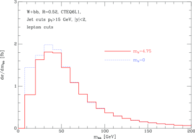
The $b\overline{b}$ pair invariant mass distribution peaks at low values of the mass due to the gluon propagator. This can be seen in Figure 3, where we show the lowest order prediction using MCFM. For $W+2$ jet production, $t$-channel dijet production dominates so that the dijet masses will in general be higher for $Wjj$ than for $Wb\overline{b}$ final states. Indeed, this is the case as can be observed in Figure 4, where the ratio of $Wb\overline{b}/Wjj$ is plotted as a function of the dijet mass.

Figure 3: The $b\overline{b}$ invariant mass in $Wb\overline{b}$ events, using lowest order matrix elements.

Figure 4: The ratio of the cross section for $Wb\overline{b}$ to $Wjj$ production as a function of the dijet mass.

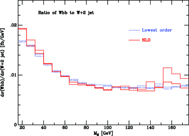
The Feynman diagram topologies may give some indication of reasonable values for the renormalization and factorization scales to use for the matrix element evaluation at leading order. The next-to-leading order result may provide further evidence to support a particular scale(s) deemed appropriate at leading order.

3 Partonic Cross Sections and Jet Algorithms

MCFM is a parton-level event generator with at most 3 partons in the final state. No information is available at the hadron level; thus any jet algorithms must be applied to the 1 or 2 partons that comprise any of the predicted final state jets.

Thus far in Run II, W+jet cross sections have been measured only with cone jet algorithms (although the ultimate goal is to also utilize $k_{T}$ algorithms as well). There are two options: the Run I legacy algorithm (JetCLU) and the joint CDF-D0 Run II algorithm (midpoint). The midpoint algorithm is so-named because it places a seed at the energy-weighted midpoint between two partons, something the JetClu algorithm does not. The midpoint algorithm also lacks the JetClu feature of “ratcheting”, where seed towers initially in the jet cone are added to the final jet energy, even if the final cone should not nominally include these towers.  Such an effect is difficult to model at the partonic level. The two effects end up being in the opposite direction so the differences between the two algorithms should be small (5% or less). One notable difference between the two algorithms is that the midpoint algorithm is defined in terms of the transverse momentum ($p_{T}$) rather than the transverse energy ($E_{T}$). Details of the application of the two algorithms to partonic level cross sections can be found in Ref. [21]. For historical reasons, the cross sections generated thus far using MCFM have used a $k_{T}$ algorithm using parameters similar to a cone algorithm of radius 0.4; however, this should not affect any of the conclusions of this paper. Calculations using cone algorithms, appropriate for direct comparisons to the measured Run 2 cross sections, are the subject of current study [22].

Jet energies measured in the CDF detector have to be corrected for comparison to theoretical predictions. The level of correction can be tricky for comparison to calculations at the NLO level. For example, one does not want to correct for the energy deposited out-of-cone due to perturbative gluon emission, since this is already accounted for to some level in the theoretical calculation. A correction should be made, however, for hadronization out-of-cone effects, since these are not present in the partonic calculation. The average hadronization correction per jet is on the order of $1$ GeV.

4 Scale Dependence

In Figure 5, the scale dependence for $Wb\overline{b}$ and $Wjj$ production is shown using cuts similar to those used in CDF [23]:

$$R_{cone}=0.4,\quad\Delta R>0.52,\quad p_{T}^{jet}>15~{}{\rm GeV},\quad|\eta_{jet}|<2.$$ (1)

For this calculation, the renormalization and factorization scales have been set equal. In perturbative QCD the freedom exists to set the two scales separately, however we have chosen not to do so at this stage. For inclusive cross sections, there is not the freedom to change the renormalization scale independently at each vertex, in contrast to a parton shower Monte Carlo where the scales at each vertex may be different. In Section 7, we will consider the impact of applying separate factorization and renormalization scales.

Figure 5: The scale dependence for LO, NLO exclusive and NLO inclusive $Wb\overline{b}$ and $Wjj$ production, using our usual set of cuts. The renormalization and factorization scales are equal.

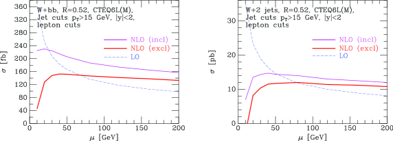
In the calculations performed with MCFM, we distinguish between exclusive and inclusive production, depending on whether there are exactly two, or two or more jets that satisfy the kinematic cuts. Contributions to three-jet final states arise only from the tree level $Wb\overline{b}j(Wjjj)$ diagrams.

The leading order cross sections for both processes decrease monotonically as the renormalization/factorization scale increases. Both the strong coupling constant $\alpha_{s}$ and the parton distribution functions (in the relevant kinematic range) decrease with increasing scale. At NLO, the scale dependence is reduced for both processes and for both inclusive and exclusive production. The logarithms that are responsible for the large variations under change of scale at leading order are exactly cancelled through next-to-leading order; any remaining scale dependence is at higher order still.

At NLO, the cross section typically increases slightly as the scale decreases and then at some point peaks and then drops with decreasing scale, due primarily to the same logarithms that cancel out the scale dependence to NLO. The exact point at which the maximum of the cross section occurs depends both on the process under consideration as well as the kinematic cuts, for example the minimum jet transverse momentum.

The scale dependence for $W+2$ jets seems to be under good control for both the inclusive and exclusive final states, as long as a scale larger than $30$ GeV is chosen. For exclusive $Wb\overline{b}$ production, the scale dependence is also reasonably small for scales larger than $30$ GeV, but a considerable scale dependence remains for inclusive final states. This is due to the relatively large number of new channels (with $gq,gg$ initial states) available for $Wb\overline{b}j$ production at NLO, and the fact that these processes are only calculated at tree level and thus have a leading order scale dependence.

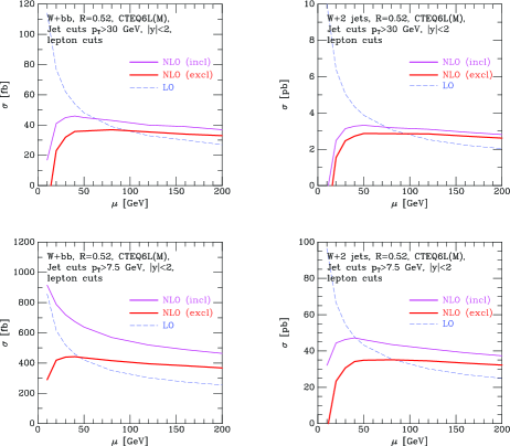
It is interesting to examine the impact of changing the kinematic cuts on the stability of the NLO calculation. In Figure 6, the study is repeated requiring the jet threshold to be $7.5$ GeV and $30$ GeV. As expected, the inclusive scale dependence gets worse (better) for the $7.5$ GeV ($30$ GeV) jet cut, as the $3$-parton final state contribution increases (decreases). Note that for $Wb\overline{b}$, the scale at which the NLO cross section becomes unstable moves to higher values as the jet transverse momentum cut increases.

Figure 6: The scale dependence for LO, NLO exclusive and NLO inclusive $Wb\overline{b}$ and $Wjj$ production when using a higher jet $p_{T}$ cut of $30$ GeV (upper plots) and a lower value of $7.5$ GeV (below).

The $K$-factors (NLO/LO) are shown in Figure 7 for $Wb\overline{b}$ and $Wjj$ exclusive final states for the three different jet transverse momentum cuts. The point at which the NLO cross section equals the LO cross section (i.e. the $K$-factor is $1$) is relatively insensitive to the jet transverse momentum cuts for the case of $Wjj$ but systematically moves out to higher scale values for $Wb\overline{b}$ production as the jet $p_{T}$ cut increases. For a scale of $100$ GeV and for a jet $p_{T}$ cut of $15$ GeV, the $Wb\overline{b}$ $K$-factor is $1.15$ while the $Wjj$ $K$-factor is $1.05$.

Figure 7: $K$-factors for $Wb\overline{b}$ (solid curves) and $Wjj$ (dotted) for exclusive final states for the 3 different jet transverse momentum cuts.

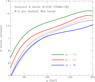
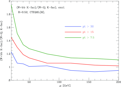
It is also interesting to plot the ratio of the $K$-factors of the two processes ($Wb\overline{b},Wjj$) as a function of the scale. The ratio of $K$-factors, shown in Figure 8, has a strong dependence on the jet $p_{T}$ cut because the $Wb\overline{b}$ $K$-factor does. The ratio is observed to be relatively constant for scales on the order of $100$ GeV or above. The ratio is particularly unstable for low scales.

Figure 8: The ratio of the $K$-factors for the two processes, as a function of the common renormalization and factorization scale $\mu$.

5 Top Physics

5.1 Two Jet Bin

One of the most promising channels for searching for $t\overline{t}$ events is a final state consisting of a high $p_{T}$ lepton plus missing transverse energy plus jets. The $W$ boson from one of the tops has decayed into a an electron or muon and neutrino while the $W$ from the other top has decayed into two quarks. Thus, there will be $4$ partons in the final state and one expects $t\overline{t}$ final states to have their largest contributions in the $W+3,4$ jet bins, depending on the jet transverse momentum cuts. Lacking NLO calculations of $Wb\overline{b}jj$ final states, CDF has estimated the number of non-$t\overline{t}$ events in the $W+$ jets sample by calculating the theoretical ratio of the $Wb\overline{b}+(n-2)$ jet cross section to the $W+n$ jet cross section ($n=2,3,4$) and then multiplying this ratio by the observed number of jets in the $W+n$ jet bin. Individually, such LO cross sections of course have a large scale dependence and thus a large uncertainty. The hope is that the $K$-factors and the scale dependence will be similar for the two processes and thus the LO ratio will be an accurate estimate of the NLO one. In CDF, this has been known as $\it Method~{}2$. Such assumptions can be explicitly tested in the $Wb\overline{b}/Wjj$ case. In Figure 8, the ratio of the K-factors for the exclusive processes $Wb\overline{b}$ and $Wjj$ were plotted as a function of the scale for three different jet $p_{T}$ cuts. For Method 2 to be accurate, the ratio should be near unity. This is true ($K_{Wb\overline{b}}/K_{Wjj}=1.05$) for a jet $p_{T}$ cut of $15$ GeV, but perhaps a kinematic accident rather than a God-given truth. It is not true for for any scale for a $p_{T}$ cut of $7.5$ GeV nor for small scales ($20-30$ GeV) for any jet $p_{T}$ cut.

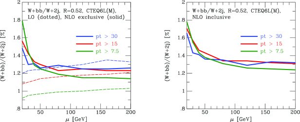
The ratio of the $Wb\overline{b}/Wjj$ cross sections is shown in Figure 9 for both exclusive and inclusive production. For both cases, the ratio is examined as a function of the minimum cut on the jet transverse momentum. It is interesting to note that for low scales, the ratio is more stable at LO than at NLO. As noted earlier, this is due to the relatively large amount of tree-level three-parton final states that enter into the $Wb\overline{b}$ process at NLO. At NLO, the ratio $Wb\overline{b}/Wjj$ is approximately $1.25$% for a $15$ GeV jet cut, while at LO this ratio is $1.18$% (but again very sensitive to the kinematic cuts). For lower scales, the discrepancy is much more extreme. At LO, the ratio has a strong dependence on the jet transverse momentum cut; this dependence is greatly reduced at NLO. A scale of approximately $100$ GeV is in the region of stability at NLO. For this scale, for a jet $p_{T}$ cut of $15$ GeV, the $K$-factor is also on the order of unity (as already noted). The inclusive ratio also has the instability at small scales and is approximately $0.1$ higher than the exclusive case for all scale values.

The exclusive NLO ratio for $Wb\overline{b}/Wjj$ of $1.25$% calculated at the scale of $100$ GeV is larger by a factor of $1.4$ than the value assumed for the $2$ jet bin using ALPGEN at LO in the CDF Run II top analysis [23]. However, it is in good agreement with the value calculated for the $2$ jet bin in Run I, after an empirical factor of $1.4$, determined from jet data [24], is applied. Thus, this analysis can be considered as a validation of the factor of $1.4$. Note that the leading order value of the ratio in the $2$ jet bin in this analysis is larger than the value observed in ALPGEN. This may be due in part to the $b$ quark being massless in this analysis, but not in the ALPGEN calculation.

Figure 9: The ratio of the $Wb\overline{b}/Wjj$ cross sections for exclusive and inclusive production.

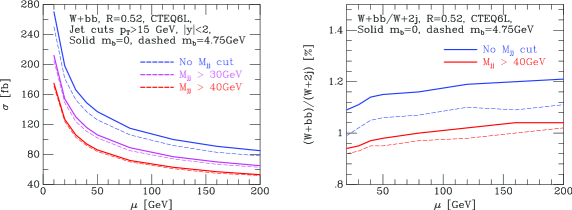
It was noted earlier that the $b\overline{b}$ mass peaks more strongly at low mass than does the dijet mass. We also examine the lowest order $Wb\overline{b}/Wjj$ ratio requiring $m_{b\overline{b}}$ ($m_{jj}$) be greater than $20$, $30$ and $40$ GeV, as shown in Figure 10. As expected, the ratio $Wb\overline{b}/Wjj$ decreases as the $b\overline{b}$ mass cut is increased. Furthermore, the impact of neglecting the $b$ mass in the calculation decreases as the $b\overline{b}$ mass cut is increased.

Figure 10: The effect of a dijet mass cut on $Wb\overline{b}$ cross section and on the $Wb\overline{b}/Wjj$ ratio.

5.2 Higher Jet Multiplicity Bins and Kinematical Analyses

NLO calculations are not yet available for the $3$ and $4$ jet bins; however, the inclusive ratio for $Wb\overline{b}/Wjj$ does give us some information about these higher jet multiplicity states. The topology of $Wb\overline{b}+(n-2)$ jet final states still remains fundamentally different from $W+n$ jet final states because of the importance of the $g\rightarrow b\overline{b}$ vertex in the former. Gluon splitting is a negligible contribution to the $W+$ jets sample. The strong scale dependence observed for $Wb\overline{b}+2$ jets at NLO may lead to some wariness about predictions for the behavior of higher jet multiplicity states. However, as we have argued, the scale sensitivity results from the relative importance of the $Wb\overline{b}$ +jet tree level diagrams; this will not happen at NLO for the $3$ or $4$ jet bin. In lieu of NLO higher jet multiplicity calculations, we can try to form observables from suitably inclusive quantities for which the NLO $Wb\overline{b}$ and $Wjj$ calculations may form an adequate approximation. One such observable is $H_{T}$; here, $H_{T}$ is defined as the sum of the transverse momenta of all of the jets, the lepton and the missing $p_{T}$ in the event. The $H_{T}$ distributions for $Wb\overline{b}(j)$ and $Wjj(j)$ are plotted in Figure 11. The (LO) distributions for $Wb\overline{b}j$ and $Wjjj$ naturally peak at at a higher value of $H_{T}$ due to the requirement of an additional jet.

For $Wjj$ the $H_{T}$ distributions are similar at LO and NLO. The $Wb\overline{b}$ distribution is steeper at LO than at NLO. In Figure 12, the cross sections for $Wb\overline{b}$ and $Wjj$ are normalized for shape comparison. There it can be clearly observed that, although, the $Wb\overline{b}$ and $Wjj$ shapes are similar at LO, the $Wjj$ distribution is steeper than that of $Wb\overline{b}$ at NLO. Any assumption that the shapes of the two processes are similar (as for example in some kinematical analyses) can be dangerous.

Figure 11: The $H_{T}$ distributions for $Wb\overline{b}(j)$ (lower curves) and $Wjj(j)$ (upper curves).

Figure 12: The $H_{T}$ distributions for $Wb\overline{b}(j)$ and $Wjj(j)$, normalized to the same area.

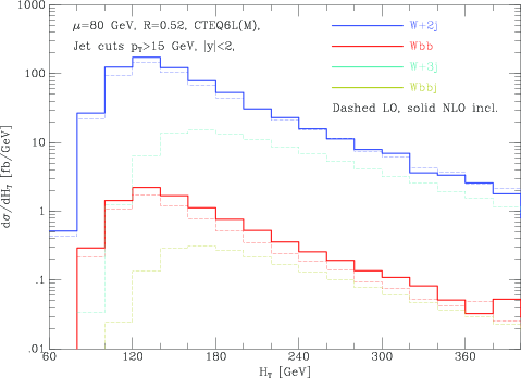
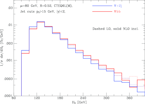
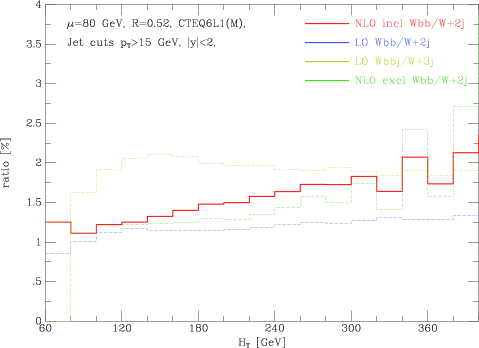
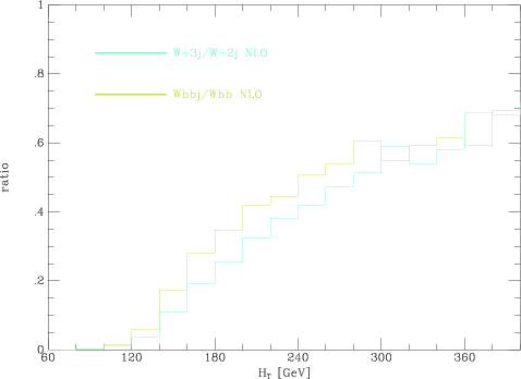
In Figure 13, the ratio of $Wb\overline{b}$ to $Wjj$, at LO and NLO (both inclusive and exclusive), as well as the (LO) ratio of $Wb\overline{b}j$ to $Wjjj$ is plotted as a function of $H_{T}$. Here, the similarity of the $Wb\overline{b}$ and $Wjj$ distributions at LO can be clearly observed, as well as the fact that the NLO ratio of $Wb\overline{b}$ to $Wjj$ increases by more than a factor of two over the $H_{T}$ range of the plot (which is approximately the same as the $H_{T}$ range used in the top analysis). Similar results to those above have also been obtained when replacing $H_{T}$ by the scalar sum of the jet transverse energies.

Figure 13: The ratio of the $H_{T}$ distributions for $Wb\overline{b}(j)$ and $Wjj(j)$.

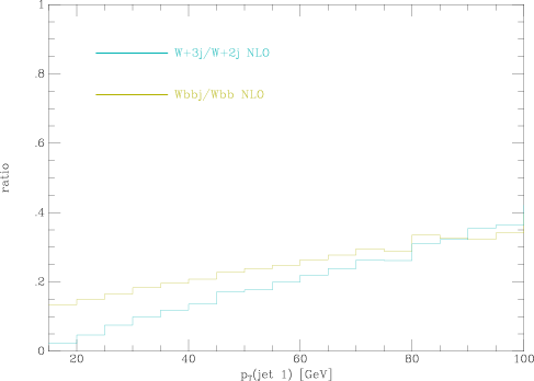
Given the shape differences between LO and NLO observed for global variables such as these, it is important to discover if the effects are the same for less inclusive observables. In Fig. 14 the ratio of $Wb\overline{b}$ to $Wjj$ is plotted as a function of the lead jet $p_{T}$. In contrast to the previous cases, the ratio is flat at NLO for both inclusive and exclusive final states. Thus, this is an example of a variable which appears to be safe with regard to a change of shape at NLO.

Figure 14: The $p_{Tjet1}$ distributions for $Wb\overline{b}(j)$ and $Wjj(j)$.

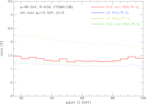
In Figs. 15 and 16 we show the relative contributions to the NLO $H_{T}$ and largest jet $p_{T}$ cross sections of the $Wb\overline{b}(Wjj)$ and $Wb\overline{b}j(Wjjj)$ subprocesses. In the NLO inclusive results, the contribution to the $H_{T}$ distribution for $Wb\overline{b}j$ and $Wjjj$ events is negligible at small $H_{T}$ and dominant at large $H_{T}$, leading to the change in shape seen in Fig. 13. This can be contrasted with the extra jet contribution to the largest jet $p_{T}$ distribution, which is never dominant over the range shown.

Figure 15: The relative contributions to the NLO $H_{T}$ cross section of the $Wb\overline{b}(Wjj)$ and $Wb\overline{b}j(Wjjj)$ subprocesses.

Figure 16: The relative contributions to the largest jet $p_{T}$ cross section of the $Wb\overline{b}(Wjj)$ and $Wb\overline{b}j(Wjjj)$ subprocesses.

6 Two Scale Studies

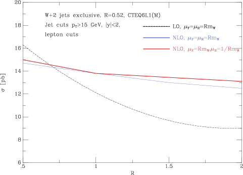
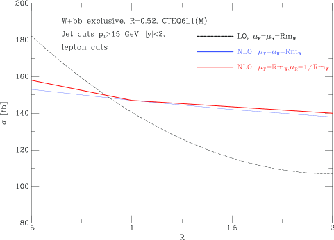
Thus far, we have set the renormalization and factorization scales to the same value. A version of MCFM has been modified to allow the separation of the two scales. In Figure 17, the $Wjj$ cross section has been plotted with the two scales set the same (both at LO and NLO) as well as for one scale pre-factor being set to the inverse of the other (at NLO). A similar plot is shown in Figure 18 for the case of $Wb\overline{b}$. As expected, the scale dependence is large at leading order; at NLO the cross section is reasonably stable for all of the scale choices plotted. Thus, the ratio of the two cross sections used in Method 2 should also be stable at NLO for the case of unequal renormalization and factorization scales and there is no anomalous enhancement of the $Wb\overline{b}$ cross section at low renormalization scales.

Figure 17: The scale dependence of the $Wjj$ exclusive cross-section, using our usual choice of varying renormalization and factorization scales together ($\mu_{F}=\mu_{R}=R\,M_{W}$, for $1/2<R<2$), as well as the choice of varying them in opposite directions ($\mu_{F}=R\,M_{W},\mu_{R}=1/R\,M_{W}$).

Figure 18: The scale dependence of the $Wb{\bar{b}}$ exclusive cross-section, using our usual choice of varying renormalization and factorization scales together ($\mu_{F}=\mu_{R}=R\,M_{W}$, for $1/2<R<2$), as well as the choice of varying them in opposite directions ($\mu_{F}=R\,M_{W},\mu_{R}=1/R\,M_{W}$).

7 Other Theoretical Uncertainties

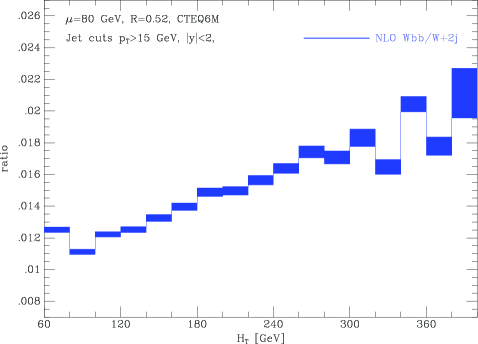
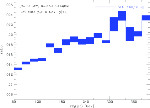
One measure of possible NNLO corrections is supplied by the scale dependence that remains at NLO. This was shown in Figures 4-9 where it was observed that the scale sensitivity is under control for choice of scale larger than $50$ GeV or so and for reasonably large jet $E_{T}$ cuts. The ratio can also be sensitive to the choice of parton distribution functions (PDF’s). We have used the $40$ error PDF’s supplied with the CTEQ6M central fit PDF to estimate the contribution of PDF uncertainty to the ratio of $Wb\overline{b}$ to $Wjj$ production. As noted earlier, different initial states contribute to the two different processes, so that PDF uncertainties will not necessarily cancel. This is the first time (that we know of) that such a study has been carried out for $Wb\overline{b}/Wjj$ final states. In order to more easily calculate the PDF uncertainties, we have used the LHAPDF interface provided in the most recent version of MCFM [25]. With this version, the parton luminosities for each PDF member can be calculated very quickly at each Monte Carlo integration point. Thus, the cross sections using all members of a given PDF set can be calculated in one Monte Carlo run. The integration is weighted by the central PDF luminosity and the result for each error set is recorded separately.

The PDF uncertainties thus calculated are shown in Figs. 19 and 20 for the $H_{T}$ and largest jet $p_{T}$ variables. The PDF uncertainties are reasonably small.

Figure 19: The PDF uncertainty for the ratio of $Wb\overline{b}$ and $Wjj$, plotted as a function of $H_{T}$, calculated using the CTEQ6 error PDF set.

Figure 20: The PDF uncertainty for the ratio of $Wb\overline{b}$ and $Wjj$, plotted as a function of the sum of the jet transverse energies, calculated using the CTEQ6 error PDF set.

8 Conclusions and Future Plans

Method 2 has proven to be a useful tool for CDF analyses both in Run 1 and in Run 2. In this paper, we have shown that Method 2 holds its validity at NLO for non-inclusive variables, for jet $E_{T}$ cuts of the order of $15$ GeV or greater, and for renormalization/factorization scales of the order of the $W$ mass.

In an ideal world, we would have available NLO calculations of $Wjjj$, $Wjjjj$, $Wb\overline{b}j$ and $Wb\overline{b}jj$. Since their availability within the next year is unlikely, we will have to continue to rely upon LO predictions of these final states. In a future paper [22], we will attempt to use the NLO processes within MCFM to directly compare MCFM predictions to (1) $Wjj$ and $Wb\overline{b}$ observables in CDF Run 2 data and (2) to enhanced LO predictions (for example using the CKKW scheme). Good agreement with the latter for $Wjj$ and $Wb\overline{b}$ final states may give some confidence in the extrapolation to higher jet multiplicity final states.  In particular, it is believed that some explicit higher order corrections are incorporated into the Sudakov form factors through the use of the CKKW procedure. We can try to explicitly test this.