hep-ph/0405244

MADPH–04–1376

UPR–1043T

UCD–2004–20

The Higgs Sector in a $U(1)^{\prime}$ Extension of the MSSM

Tao Han^1,4, Paul Langacker², Bob McElrath^{3 1}Department of Physics, University of Wisconsin, Madison, WI 53706

²Department of Physics and Astronomy, University of Pennsylvania, Philadelphia, PA 19104
³Department of Physics, University of California, Davis, CA 95616

⁴Institute of Theoretical Physics, Academia Sinica, Beijing 100080, China

Abstract

We consider the Higgs sector in an extension of the MSSM with extra SM singlets, involving an extra $U(1)^{\prime}$ gauge symmetry, in which the domain-wall problem is avoided and the effective $\mu$ parameter is decoupled from the new gauge boson $Z^{\prime}$ mass. The model involves a rich Higgs structure very different from that of the MSSM. In particular, there are large mixings between Higgs doublets and the SM singlets, significantly affecting the Higgs spectrum, production cross sections, decay modes, existing exclusion limits, and allowed parameter range. Scalars considerably lighter than the LEP2 bound (114 GeV) are allowed, and the range $\tan\beta\sim 1$ is both allowed and theoretically favored. Phenomenologically, we concentrate our study on the lighter (least model-dependent, yet characteristic) Higgs particles with significant $SU(2)$-doublet components to their wave functions, for the case of no explicit $CP$ violation in the Higgs sector. We consider their spectra, including the dominant radiative corrections to their masses from the top/stop loop. We computed their production cross sections and reexamine the existing exclusion limits at LEP2. We outline the searching strategy for some representative scenarios at a future linear collider. We emphasize that gaugino, Higgsino, and singlino decay modes are indicative of extended models and have been given little attention. We present a comprehensive list of model scenarios in the Appendices.

I Introduction

Supersymmetry (SUSY) is probably the leading candidate for physics beyond the Standard Model (SM). By adding partners of opposite statistics to the SM particles, it is able to cancel the quadratically divergent contribution to the Higgs mass. The leading phenomenological model for SUSY is the Minimal Supersymmetric Standard Model (MSSM), which incorporates two Higgs doublets rather than one as in the Standard Model. Two are required to give masses to both up-type and down-type fermions, and to prevent anomalies coming from triangle diagrams involving the Higgs superpartner, the Higgsino.

The MSSM suffers from the “$\mu$ problem” muprob . The superpotential for the MSSM contains the supersymmetric mass term $\mu H_{2}H_{1}$. The minimization condition for the MSSM scalar potential relates $\mu$ to $M_{Z}$ and soft SUSY breaking parameters. One expects all these quantities to be the same order of magnitude to avoid the need for miraculous cancellations. However, $\mu$ is an input-scale parameter and therefore should have mass ${\mathcal{O}}(M_{Pl})$ or ${\mathcal{O}}(M_{GUT})$. This has led to a widespread belief that the MSSM must be extended at high energies to include a mechanism which relates $\mu$ to the SUSY breaking mechanism.

One possibility is the next-to-minimal Supersymmetric Standard Model (NMSSM) nmssm , which has been studied extensively nmssm ; nmssmpheno . The NMSSM solves the $\mu$ problem by relating $\mu$ to the vacuum expectation value of a Standard Model singlet. The model contains a single extra gauge singlet superfield, $S$, and a superpotential of the form:

$$W_{NMSSM}={1\over 6}kS^{3}+{1\over 2}\mu_{S}S^{2}+hSH_{2}H_{1}+W_{MSSM},$$ (1)

where $W_{MSSM}$ is the superpotential of the MSSM without an elementary $\mu$ term . If the scalar component of $S$ has a vacuum expectation value, an effective $\mu$ term $h\langle S\rangle$ is induced. However, to have the appropriate hierarchy of mass scales, the term $\mu_{S}$ should be disallowed. Otherwise, it should also naturally have a mass near $M_{Pl}$, which would make it unnatural for $S$ to obtain a weak-scale vacuum expectation value. Similar statements apply to the addition of a term linear in $S$ to $W_{NMSSM}$. These can be removed by invoking a $Z_{3}$ discrete symmetry in the superpotential. However this would lead to domain walls in the early universe, a situation which is strongly disfavored cosmologically domains . Attempts to remedy this either reintroduce some form of the $\mu$ problem or lead to other difficulties domains2 .

In string motivated models, bare mass terms in the superpotential are generically of order the string scale $M_{\rm string}$. This means that any field impacting low energy physics must not have a mass term like $\mu$ or $\mu_{S}$. Additionally, in many constructions (e.g., heterotic and intersecting brane) superpotential terms are typically off-diagonal in the fields, which disallows the NMSSM $kS^{3}$ term. Thus, we are led to consider larger models that may be derived from string constructions.

All of these difficulties can be solved in extended models involving an additional (non-anomalous) $U(1)^{\prime}$  gauge symmetry, which is very well-motivated as an extension to the MSSM. $U(1)$ gauge groups arise naturally out of many Grand Unified Theories (GUT’s) and string constructions string , as do the SM singlets needed to break the $U(1)^{\prime}$. Experimental limits on the $Z^{\prime}$ mass and mixings are model-dependent, but typically one requires zprimeev ; CDFzprime $\mbox{$M_{Z^{\prime}}$}>500-800$ GeV and a $Z-Z^{\prime}$ mixing smaller than a few $\times 10^{-3}$.

$U(1)^{\prime}$  models are similar to the NMSSM in that they involve a SM singlet field $S$ which yields an effective $\mu$ parameter $h\langle S\rangle$, where the superpotential includes the term $hSH_{2}H_{1}$, solving the $\mu$ problem mugauge ; mugauge2 . $S$ will in general be charged under the $U(1)^{\prime}$  gauge symmetry, so that its expectation value also gives mass to the new $Z^{\prime}$ gauge boson. The extended gauge symmetry forbids an elementary $\mu$ term as well as terms like $S^{n}$ in the superpotential (the role of the $S^{3}$ term in generating quartic terms in the potential is played by $D$-terms and possibly off-diagonal superpotential terms involving additional SM singlets). Such models do not need to invoke discrete symmetries (the $Z_{3}$ of the NMSSM is embedded in the $U(1)^{\prime}$) so there are no domain wall problems. Such constructions may also solve other problems, such as naturally forbidding $R$-parity violating terms which could lead to rapid proton decay chiral . Other implications include the presence of exotic chiral supermultiplets chiral ; non-standard sparticle spectra alternative ; possible flavor changing neutral current effects FCNC , with implications for rare $B$ decays bdecay ; new sources of CP violation CP ; new dark matter candidates darkmatter ; and enhanced possibilities for electroweak baryogenesis elbary .

As mentioned, string constructions frequently lead to the prediction of one or more additional $U(1)^{\prime}$ symmetries at low energies and to the existence of exotic chiral supermultiplets, including SM singlets which can break the extra symmetries. However, no fully realistic model has emerged. We therefore take the bottom-up approach and add the minimal supersymmetric matter content necessary to solve the $\mu$ problem without introducing extra undesirable global or discrete symmetries.

In this paper we explore the extended Higgs sector in a particular $U(1)^{\prime}$ model involving several SM singlet fields ell . This has the advantage of decoupling the effective $\mu$ parameter from the $Z^{\prime}$ mass, and leads naturally to a sufficiently heavy $Z^{\prime}$. It will be seen that the Higgs physics is very rich and quite different from that of the MSSM. We expect that the generic features will be representative of a wider class of constructions, and that they can be tested by the next generation of high energy experiments and thus provide further guidance toward constructing the correct SUSY theory. In the event that the data from the LHC deviates significantly from MSSM expectations, it will be especially important to consider non-minimal models. It is useful in planning for future experimental analysis programs to have a variety of well-motivated alternatives in mind.

In Section II we describe the model. We first outline the general structure of the model in Sec. II.1, and discuss the electroweak symmetry breaking and the radiative corrections to the light Higgs mass in Sec. II.2. We then explore the phenomenological constraints on the model parameters in Sec. III. In particular, we find that the MSSM upper bound on the light Higgs mass and the lower bound (direct search from LEP2) can both be relaxed. In order to carry out further quantitative studies, we perform a comprehensive examination of the mass spectrum for the Higgs bosons in Sec. IV. We classify the Higgs bosons according to their similarity to the MSSM spectrum and experimental signatures. The decay modes of the Higgs bosons and their production cross sections at $e^{+}e^{-}$ colliders are studied in Sec. V, including phenomenological implications and search strategies. We summarize our results in Sec. VI.

II The Model

II.1 General structure

The model we consider, first introduced in ell , has the superpotential:

$$W=hSH_{2}H_{1}+\lambda S_{1}S_{2}S_{3}+W_{\rm MSSM}$$ (2)

$S$, $S_{1}$, $S_{2}$, and $S_{3}$ are standard model singlets, but are charged under an extra $U(1)^{\prime}$ gauge symmetry. The off-diagonal nature of the second term is inspired by string constructions, and the model is such that the potential has an $F$ and $D$-flat direction in the limit $\lambda\rightarrow 0$, allowing a large (TeV scale ) $Z^{\prime}$ mass for small $\lambda$. The use of an $S$ field different from the $S_{i}$ in the first term allows a decoupling of $M_{Z^{\prime}}$ from the effective $\mu$. $W$ leads to the $F$-term scalar potential:

$$V_{F}= h^{2}\left(|H_{2}|^{2}|H_{1}|^{2}+|S|^{2}|H_{2}|^{2}+|S|^{2}|H_{1}|^{2}\right)$$

$$+ \lambda^{2}\left(|S_{1}|^{2}|S_{2}|^{2}+|S_{2}|^{2}|S_{3}|^{2}+|S_{3}|^{2}|S_{1}|^{2}\right)$$ (3)

The $D$-term potential is:

$$V_{D} = {{G^{2}}\over 8}\left(|H_{2}|^{2}-|H_{1}|^{2}\right)^{2}$$ (4)

$$+ {1\over 2}g_{Z^{\prime}}^{2}\left(Q_{S}|S|^{2}+Q_{H_{1}}|H_{1}|^{2}+Q_{H_{2}}|H_{2}|^{2}+\sum_{i=1}^{3}Q_{S_{i}}|S_{i}|^{2}\right)^{2}~{},~{}\,$$

where $G^{2}=g_{1}^{2}+g_{2}^{2}=g_{2}^{2}/\cos^{2}\theta_{W}$. $g_{1},g_{2}$, and $g_{Z^{\prime}}$ are the coupling constants for $U(1),SU(2)$ and $U(1)^{\prime}$, respectively, and $\theta_{W}$ is the weak angle. $Q_{\phi}$ is the $U(1)^{\prime}$ charge of the field $\phi$. We will take $g_{Z^{\prime}}\sim\sqrt{5/3}g_{1}$ (motivated by gauge unification) for definiteness.

We do not specify a SUSY breaking mechanism but rather parameterize the breaking with the soft terms

$$V_{\rm soft} = m_{H_{1}}^{2}|H_{1}|^{2}+m_{H_{2}}^{2}|H_{2}|^{2}+m_{S}^{2}|S|^{2}+\sum_{i=1}^{3}m_{S_{i}}^{2}|S_{i}|^{2}$$ (5)

$$- (A_{h}hSH_{1}H_{2}+A_{\lambda}\lambda S_{1}S_{2}S_{3}+{\rm H.C.})$$

$$+ (m_{SS_{1}}^{2}SS_{1}+m_{SS_{2}}^{2}SS_{2}+{\rm H.C.})$$

The last two terms are necessary to break two unwanted global $U(1)$ symmetries, and require $Q_{S_{1}}=Q_{S_{2}}=-Q_{S}$. The potential $V=V_{F}+V_{D}+V_{soft}$ was studied in ell , where it was shown that for appropriate parameter ranges it is free of unwanted runaway directions and has an appropriate minimum. We denote the vacuum expectation values of $H_{i},S,$ and $S_{i}$ by $v_{i},v_{s},$ and $v_{si}$, respectively, i.e., without a factor of $1/\sqrt{2}$. Without loss of generality we can choose $A_{h}h>0$, $A_{\lambda}\lambda>0$ and $m^{2}_{SS_{i}}<0$ in which case the minimum occurs for the expectation values all real and positive.

So far we have only specified the Higgs sector, which is the focus of this study. Fermions must also be charged under the $U(1)^{\prime}$ symmetry in order for the fermion superpotential Yukawa terms $W_{fermion}=\bar{u}{\bf y_{u}}QH_{2}-\bar{d}{\bf y_{d}}QH_{1}-\bar{e}{\bf y_{e}}LH_{1}$ to be gauge invariant. The $U(1)^{\prime}$ charges for fermions do not contribute significantly to Higgs production or decay, if sfermions and the $Z^{\prime}$ superpartner are heavy. We therefore ignore them this study.

Anomaly cancellation in $U(1)^{\prime}$ models generally requires the introduction of additional chiral supermultiplets with exotic SM quantum numbers mugauge2 ; chiral ; elbary ; wang . These can be consistent with gauge unification, but do introduce additional model-dependence. The exotics can be given masses by the same scalars that give rise to the heavy $Z^{\prime}$ mass. The exotic sector is not the focus of this study. We therefore consider the scenario in which the $Z^{\prime}$ and other matter necessary to cancel anomalies is too heavy to significantly affect the production and decays of the lighter Higgs particles.

II.2 Higgs sector and electroweak symmetry breaking

The Higgs sector for this model contains 6 CP-even scalars and 4 physical CP-odd scalars, which we label $H_{1}...H_{6}$ and $A_{1}...A_{4}$, respectively, in order of increasing mass.

We compute the six CP-even scalar masses including the dominant 1-loop contribution coming from the top/stop loop. Using the effective potential approach effpot , one writes down the radiatively corrected effective potential including leading order (0) and 1-loop corrections (1)

$$V_{\rm eff}=V^{(0)}+V^{(1)}+...$$ (6)

and then requires that the effective potential be minimized to obtain the vacuum expectation values for the fields. In practice we find it simpler to eliminate the soft $(\rm mass)^{2}$ parameters using the minimization conditions rather than solve for vacuum expectation values.

The full scalar potential is then

$$V_{\rm eff}=V_{D}+V_{F}+V_{\rm soft}+\frac{3}{16\pi^{2}}\frac{m_{t}^{4}}{v^{4}}(v_{2}^{2}+v_{1}^{2})^{2}\left(\frac{\Re H_{2}}{\sqrt{2}v_{2}}+1\right)^{4}\left\{\frac{3}{2}-\ln{\left[\frac{m_{t}^{2}}{m_{\tilde{t}}^{2}}\left(\frac{\Re H_{2}}{\sqrt{2}v_{2}}+1\right)^{2}\right]}\right\}$$ (7)

At one loop only the $H_{2}$ gauge eigenstate gets a correction. At two loops both $H_{1}$ and $H_{2}$ get corrections from the top and stop. We have written $v$, $v_{1}$ and $v_{2}$ in such a way so that $v_{1}$ and $v_{2}$ can be considered rescaled quantities, while $v,m_{t},$ and $m_{\tilde{t}}$ (which only occur in ratios) are fixed at their physical values (as given in Table 1). To avoid computational round-off error we treat $V_{\rm eff}$ as a dimensionless quantity with all values ${\mathcal{O}}(1)$, and rescale dimensionful quantities by $v/\sqrt{(v_{2}^{2}+v_{1}^{2})}$ after a viable minimum is found.

In the $\Re{(H_{2},H_{1},S,S_{1},S_{2},S_{3})}$ gauge basis, the resulting mass matrix can be parameterized as $M_{tree}^{2}+\delta M^{2}$, where

$$\delta M^{2}=\left({\delta m^{2}_{H_{2}}\atop 0_{5\times 1}}{0_{1\times 5}\atop 0_{5\times 5}}\right),\hskip 56.9055pt\delta m^{2}_{H_{2}}=\frac{3}{4\pi^{2}}\frac{m_{t}^{4}}{v_{2}^{2}}\ln{m_{\tilde{t}}^{2}\over m_{t}^{2}}$$ (8)

in the no-stop mixing limit $m_{\tilde{t_{1}}}=m_{\tilde{t_{2}}}$ effpot . Since in this model $\tan\beta\simeq 1$ generically, the contribution from the bottom loop is negligible so we do not include it. We also neglect renormalization scale-dependence and assume the renormalization scale $Q^{2}=m_{\tilde{t}}^{2}$. The singlets cannot couple directly to the top at tree level, so the large top loop does not contribute to the masses of any of the new singlets except by mixing. The correction $\delta m^{2}_{H_{2}}$ has the value $(90\,\mbox{GeV})^{2}$ for the MSSM with $m_{\tilde{t}}=1\,\mbox{TeV}$ in the large $\tan{\beta}$ limit. In the MSSM this is then split among the $h$ and $H$ mass eigenstates. All other quantities are evaluated at tree level, using tree level relations.

We find viable electroweak symmetry breaking minima by scanning over the vacuum expectation values of the six CP-even scalar fields. We require that the CP-even mass matrix be positive definite numerically, which guarantees a local minima, while simultaneously eliminating the soft mass squared for each field. The soft masses reported in the appendices are evaluated including the above 1-loop correction. The CP-odd mass matrix is guaranteed to be positive semi-definite at tree level (and thus, all VEV’s are real) by appropriate redefinitions of the fields and choices of parameters as described in Sec. III.1. The expressions for the first-derivative conditions to eliminate the soft masses are given in ell . The procedure outlined guarantees a local minimum for each parameter point, but does not guarantee a global minimum.

The parameters $m_{SS_{1}}^{2}$ and $m_{SS_{2}}^{2}$ must be chosen to avoid directions in the potential that are unbounded from below. We require

$$m_{S}^{2}+m_{S_{i}}^{2}+2m_{SS_{i}}^{2}>0,$$ (9)

to avoid unbounded directions with $v_{s}=v_{si}$ and the other VEV’s vanishing.

We scan over vacuum expectation values such that the three singlets $S_{1}$, $S_{2}$, and $S_{3}$ typically have larger VEV’s than the other three fields. We allow points in our Monte Carlo scan that fluctuate from all VEV’s equal up to $\langle S\rangle$ approximately 1 TeV and $\langle S_{i}\rangle$ approximately 10 TeV, as we specify in Table 1. This generically results in a spectrum with 1-5 relatively light CP-even states, often with one of them lighter than the LEP2 mass bound, but having a relatively small overlap with the MSSM $H_{2}$ and $H_{1}$. It is necessary that at least one of the singlets have an $\mathcal{O}({\rm TeV})$ vacuum expectation value, so that the mass of the $Z^{\prime}$ gauge boson is sufficently heavy that it evades current experimental bounds, and any extra matter needed to cancel anomalies is heavy enough to not significantly affect light Higgs production or decay.

A bound exists on the mass of the lightest Higgs particle in any perturbatively valid supersymmetric theory Kane:1992kq ; Quiros:1998bz . The limit on the lightest MSSM-like CP-even Higgs mass in this model is:

$$M^{2}_{h}\leq h^{2}v^{2} + (M_{Z}^{2}-h^{2}v^{2})\cos^{2}{2\beta}+2g_{Z^{\prime}}^{2}v^{2}(Q_{H_{2}}\cos^{2}\beta+\sin^{2}\beta Q_{H_{1}})^{2}$$ (10)

$$+ {3\over 4}\frac{m_{t}^{4}}{\pi^{2}v^{2}}\ln{m_{\tilde{t_{1}}}m_{\tilde{t_{2}}}\over m_{t}^{2}}.$$

This is obtained by taking the limit as the equivalent of the $B$-term in the MSSM goes to infinity, $B=A_{h}hv_{s}\rightarrow\infty$, in the $2\times 2$ submatrix containing $H_{2}$ and $H_{1}$. In the MSSM this is equivalent to taking $M_{A}\rightarrow\infty$, the decoupling limit. This expression is the same as in the NMSSM, except for the $g_{Z^{\prime}}$ ($D$-term) contribution. Perturbativity to a GUT or Planck scale places an upper limit ${\mathcal{O}}(0.8)$ on $h$ ell , which is less stringent than the corresponding limit in the NMSSM NMSSMbnd due to the $U(1)^{\prime}$ contributions to its renormalization group equations. Larger values would be allowed if another scale entered before the Planck scale. We will allow $h$ as large as 1 in the interest of exploring the low energy effective potential. The second term of Eq. (10) vanishes for $\tan\beta=1$. Since $\tan\beta\simeq 1$ generically in these models, the lightest Higgs mass is determined mostly by the new $F$ and $D$-term contributions proportional to $h^{2}$ and $g_{Z^{\prime}}^{2}$. In this model, as with any model with many Higgs particles, a situation can arise in which the MSSM-like couplings are shared among many states, allowing unusually heavy states or unusually light states that evade current experimental bounds.

The four CP-odd masses can in principle be found algebraically but the results are complicated and not very illuminating. Perhaps the most striking feature of the mass spectrum is that the $A_{1}$ is allowed to be very light, a feature shared with the NMSSM nmssm . This is caused by a combination of small $m_{SS_{1}}^{2}$ or $m_{SS_{2}}^{2}$ and a small value of $v_{s}$ compared to the $v_{si}$. In the limit that $v_{si}\ (i=$ 1 or 2) is the largest scale in the problem, the lightest $A$ mass is

$$m_{A_{1}}^{2}=-m_{SS_{i}}^{2}\frac{v_{s}v_{si}}{v_{si}^{2}+v_{s3}^{2}}+\mathcal{O}\left(\frac{1}{v_{si}^{4}}\right).$$ (11)

In the limit that $s_{3}$ is large we obtain

$$m_{A_{1}}^{2}=-4m_{SS_{i}}^{2}\frac{v_{s}v_{si}}{v_{s}^{2}+v_{s1}^{2}+v_{s2}^{2}}+\mathcal{O}\left(\frac{1}{v_{s3}}\right).$$ (12)

In our scans, $-m_{SS_{i}}^{2}$ is approximately in the range ($0-1000$ GeV)². An example where this occurs is presented in Appendix (A-1). However, this requires a hierarchy between the off-diagonal soft masses $m_{SS_{i}}$ and the other soft masses $m_{S}$ and $m_{S_{i}}$. This might be difficult to achieve depending on the SUSY breaking mechanism. A similar analysis holds for $H_{1}$, but an algebraic expression cannot be derived since the eigenvalues of a $6\times 6$ matrix cannot be expressed algebraically. Examples of spectra with a light $H_{1}$ are given in Appendices (A-2,A-3).

To make comparisons to the MSSM, we define the “MSSM fraction” $\xi_{\rm MSSM}$. For a given Higgs state $H_{i}\ (A_{i})$ in the mass basis,

$$\xi^{i}_{\rm MSSM}=\sum_{j=1}^{2}(R^{ji})^{2},$$ (13)

where $R$ is the matrix that rotates the interaction fields to the mass basis, and the index $j$ runs over MSSM states. In the case of the CP-even Higgs this corresponds to adding in quadrature the eigenvector components of a state in the $H_{2}$ and $H_{1}$ directions. When a state is MSSM-like, $\xi_{\rm MSSM}=1$ and it has no mixing with singlet Higgs bosons. If the two lightest CP-even states and the lightest CP-odd state all have $\xi_{\rm MSSM}\simeq 1$, the theory is MSSM-like and the extra scalars are decoupled. An example of such a spectrum is presented in Appendix (A-4). There is always a massless CP-odd scalar with $\xi_{\rm MSSM}\simeq 1$, and another with $\xi_{\rm MSSM}\simeq 0$. These are the Goldstone bosons corresponding to the $Z$ and $Z^{\prime}$ gauge bosons, respectively.

A similar quantity is defined for the neutralinos by summing in quadrature over the eigenvector components corresponding to $\tilde{B}$, $\tilde{Z}$, $\tilde{H_{2}}$ and $\tilde{H_{1}}$. The “Singlino fraction” $\xi_{\tilde{s}}$ and “Zino-prime fraction” $\xi_{\tilde{Z^{\prime}}}$ are defined in an analogous manner.

III Phenomenological Constraints

Due to the introduction of the Higgs singlets, there are several more parameters than in the MSSM Higgs sector. We follow the global symmetry breaking structure of Model I of Ref. ell . Existing experimental measurements already constrain any new model. In our parameter space scans, we apply the constraints in the following subsections.

III.1 Parameter Space

$g_{1}=0.36$	$g_{2}=0.65$	$g_{Z^{\prime}}=\sqrt{5/3}g_{1}$
$m_{t}=174.3\,\mbox{GeV}$	$v=174\,\mbox{GeV}$	$m_{\tilde{t_{1}}}=m_{\tilde{t_{2}}}=1\,\mbox{TeV}$
$Q_{H_{2}}={1}/{4}$	$Q_{H_{1}}={1}/{4}$	$Q_{S}=-{1}/{2}$
$Q_{S_{1}}={1}/{2}$	$Q_{S_{2}}={1}/{2}$	$Q_{S_{3}}=-1$
$h=-1\ ...\ 1$	$\lambda=-0.2\ ...\ 0.2$
$A_{h}=0.0\ ...\ 50$	$A_{\lambda}=$0.0 … 50
$|m_{SS_{1}}^{2}|=0\ ...\ 100~{}~{}~{}$	$|m_{SS_{2}}^{2}|=$0 … 100	$m_{S_{1}S_{2}}=0$
$M_{2}=-10\ ...\ 10$	$M_{1}=-5\ ...\ 5$	$M_{1}^{\prime}=-20\ ...\ 20$
$v_{1,2}=1\ ...\ e$	$v_{s}=1\ ...\ e^{2}$	$v_{s1,2,3}=1\ ...\ e^{4}$

Table 1: Input values and the ranges for model parameters.

We list the model parameters in Table 1. Besides the SM gauge couplings, $g_{Z^{\prime}}$ is chosen as $\sqrt{5/3}g_{1}$ that unifies with $g_{2}$ and $g_{3}$ in simple GUT models. However, we do not require unification of the gaugino masses. We have fixed the $U(1)^{\prime}$ charges for definiteness. The parameters $A_{h}$, $A_{\lambda}$, $m_{SS_{1}}$, and $m_{S_{1}S_{2}}$, and $M_{2}$ are of course dimensionful, as are the expectation values $v_{i},v_{s},$ and $v_{si}$. For our computation we choose arbitrary units to start, and use the analytical minimization conditions for the VEV’s as given in Ref. ell , eliminating the soft mass square parameters. We check that the VEV’s obtained from scanning are a minimum by explicitly verifying that the matrix of second derivatives is positive definite. After finding a viable minimum, we rescale all dimensionful parameters by $v/\sqrt{v_{2}^{2}+v_{1}^{2}}$, where $v$ is fixed at 174 GeV, which shifts the Higgs vacuum expectation value to its measured value. The other dimensionful parameters $m_{t}$, $v$, $m_{SUSY}$, $m_{\tilde{t_{1}}}$ and $m_{\tilde{t_{2}}}$ enter the Higgs potential at one loop as given by Eq. (7). However, they enter in ratios so that the units cancel out. $\tan\beta=v_{2}/v_{1}$ is therefore an output.

In the MSSM the sign of $\mu$ is a free parameter. In this model $\mu=hv_{s}$, and $v_{s}$ is taken to be positive at the minimum, meaning that the sign of $\mu$ is really the sign of $h$. We can absorb any overall phase of $A_{h}h$ by a redefinition of the fields, in exactly the same way a phase of $B$ can be absorbed in the MSSM, and $B=A_{h}h$ taken to be positive. Any phase appearing in the soft-masses $-m_{SS_{1}}^{2}$ and $-m_{SS_{2}}^{2}$ can be absorbed by a field redefinition on $S_{1}$ or $S_{2}$, so that $m^{2}_{SS_{i}}$ are negative. $\lambda A_{\lambda}$ can be taken to be positive by redefining $S_{3}$. This uses up our freedom to redefine our fields, leaving a true phase in $h$ and $\lambda$ that cannot be rotated away. With these field redefinitions $A_{h}h$, $A_{\lambda}\lambda$, $-m_{SS_{1}}^{2}$, and $-m_{SS_{2}}^{2}$ are all positive , and all of the VEV’s will be real and positive at the minimum. There is not enough freedom left to rotate away a phase appearing in a possible additional term $m_{S_{1}S_{2}}^{2}S_{1}^{\dagger}S_{2}$. We have thus taken this parameter to be zero. A phase in this parameter would provide for CP violation in the Higgs sector, and therefore lead to mixing between scalars and pseudoscalars. Although such a term is useful for electroweak baryogenesis elbary , it is beyond the scope of the present investigation.

With these conventions the gaugino masses can be either positive or negative. The scalar potential and therefore vacuum expectation values are insensitive to the signs of $h$ and $\lambda$ at tree level, since it always appears as $A_{h}h$ and $A_{\lambda}\lambda$ whose phases can be rotated away, or $|h|^{2}$ and $|\lambda|^{2}$. Only the charginos and neutralinos are sensitive to the signs of $h$ and $\lambda$. The neutralino and chargino mass matrices are given in Ref. ell . We allow both positive and negative values for $h$, $\lambda$, and the gaugino masses.

III.2 $Z^{\prime}$ Mass and $Z-Z^{\prime}$ Mixing

Limits on the $Z^{\prime}$ mass and $Z-Z^{\prime}$ mixing angle are model-dependent. However, for typical models the $Z$ pole data indicate that the $Z-Z^{\prime}$ mixing must be less than a few $\times 10^{-3}$ zprimeev , while direct searches at the Tevatron limit the mass of the $Z^{\prime}$ to be greater than $\sim 500-800$ GeV CDFzprime . Therefore, we require of the $Z-Z^{\prime}$ mixing angle:

$$\alpha_{Z-Z^{\prime}}={1\over 2}\arctan\left(\frac{2M_{ZZ^{\prime}}^{2}}{M_{Z^{\prime}}^{2}-M_{Z}^{2}}\right)\mathrel{\raise 1.29167pt\hbox{$<$\kern-7.5pt\lower 4.30554pt\hbox{$\sim$}}}5\times 10^{-3}$$ (14)

where $M^{2}_{ZZ^{\prime}}$ is the off-diagonal entry in the mass-squared matrix, and $M_{Z}^{2}$, $M_{Z^{\prime}}^{2}$ are the diagonal entries. We require for the mass:

$$M_{Z^{\prime}}\geq 500\,\mbox{GeV}.$$ (15)

The $Z^{\prime}$ would be produced at tree level at the Tevatron, since if we require that fermions receive mass through the usual Higgs mechanism, they must be charged under $U(1)^{\prime}$ to keep the superpotential Yukawa terms gauge invariant. We do not calculate the $Z^{\prime}$ production cross section to avoid the necessity of having to specify the fermion $U(1)^{\prime}$ charges. This model does not particularly care how heavy the $Z^{\prime}$ is. Since there are four singlets contributing to its mass, it is not difficult to give some of them large vacuum expectation values, resulting in a heavy $Z^{\prime}$. This occurs naturally for small $\lambda$.

A lighter $Z^{\prime}$ near the experimental limit is also not a problem. The singlets must have smaller vacuum expectation values, and therefore smaller masses, but since they do not couple directly to the Standard Model except by mixing with the MSSM Higgs bosons, they can be light. The typical scale for exotics introduced to cancel anomalies is near the $Z^{\prime}$ mass.

The mixing constraint in (14) is most easily satisfied for $M_{Z^{\prime}}$ in the TeV range. Smaller values of $M_{Z^{\prime}}$, such as we allow, generally require a suppressed value for $M^{2}_{ZZ^{\prime}}=g_{Z^{\prime}}\sqrt{g^{2}+g^{\prime 2}}(Q_{H_{2}}v_{2}^{2}-Q_{H_{1}}v_{1}^{2})$. Since $\tan\beta$ is typically close to unity, this is achieved for the choice $Q_{H_{2}}=Q_{H_{1}}$, which we have assumed.

III.3 Chargino and Neutralino Mass Bounds

The chargino in this model is essentially identical to the MSSM chargino. There are no new tree-level modifications to the chargino couplings or mass. As reported by the LEP2 experiments, we require that the chargino mass be

$$M_{\chi^{\pm}}\geq 103\,\mbox{GeV}.$$ (16)

We place no constraints on the neutralino. Current constraints are very model-dependent. Even with the MSSM it has been demonstrated that the LSP can be as light as $6\,\mbox{GeV}$ Hooper:2002nq . With the additional assumption that the LSP is mostly singlet, it can be lighter still (including massless Gogoladze:2002xp ). Such light singlinos may provide a very interesting candidate for the dark matter component of the universe mySinglinoDM .

III.4 LEP2 Bounds on the Higgs Masses

The pair creation of the charged Higgs boson $H^{+}H^{-}$ in $e^{+}e^{-}$ collisions provides a model-independent channel for the Higgs search. The non-observation of this signal at LEP2 requires

$$M_{H^{\pm}}\geq 71.5\,\mbox{GeV}.$$ (17)

Limits were placed on cross sections for $e^{+}e^{-}\rightarrow Zh$ and $e^{+}e^{-}\rightarrow Ah,\ AH$ at LEP2 up to energies of 209 GeV. We impose on our model that it not violate these bounds by directly computing these cross sections. For a theory with two Higgs doublets plus any number of singlets, the cross section for a Higgs boson radiation off a $Z$ is simply related to the SM cross section by

$$\sigma(e^{+}e^{-}\rightarrow ZH^{i})=(R^{i1}_{H}\sin\beta-R^{i2}_{H}\cos\beta)^{2}\sigma_{SM}(e^{+}e^{-}\rightarrow Zh),$$ (18)

where $R_{H}$ is the matrix that diagonalizes the CP-even Higgs mass matrix. Similarly, the cross section for Higgs pair production via $Z$ exchange is obtained by scaling the MSSM result

$$\sigma(e^{+}e^{-}\rightarrow H^{i}A^{j})=(R^{i1}_{H}R^{j1}_{A}-R^{i2}_{H}R^{j2}_{A})^{2}\frac{\lambda(M_{A^{j}},M_{H^{i}})^{3/2}}{(12M_{Z}^{2}/s+\lambda(M_{Z},M_{h}))\lambda(M_{Z},M_{h})^{1/2}}\sigma_{SM}(e^{+}e^{-}\rightarrow hZ)$$ (19)

where $R_{A}$ is the matrix that diagonalizes the CP-odd Higgs mass matrix. $\lambda(m_{1},m_{2})=(1-(m_{1}+m_{2})^{2}/s)(1-(m_{1}-m_{2})^{2}/s)$. The explicit indices $1$ and $2$ correspond to the $H_{1}$ and $H_{2}$ columns, respectively. The cross section can be written in this simple form because the $ZhA$ vertex comes entirely from the covariant derivatives of $H_{2}$ and $H_{1}$.

We impose that these two cross sections be less than the LEP2 limits for all mass eigenstates with each production channel separately. For the $ZH$ case we use the LEP2 limit $M_{h}\geq 114.1\,\mbox{GeV}$, which leads to a cross section of 184 fb as an upper bound at $\sqrt{s}=209\,\mbox{GeV}$. We then require that the cross section in this model be less than that value. Since the cross section increases as the Higgs mass is decreased, this gives a conservative estimate of when a model is inconsistent with the LEP2 bound and is thus ruled out in terms of the Higgs mass and other coupling parameters. For $HA$ channels, using the LEP2 MSSM mass limits $M_{h}\leq 91.0\,\mbox{GeV}$ and $M_{A}\leq 91.9\,\mbox{GeV}$, we compute the $hA$ cross section to be $48.3$ fb at $\sqrt{s}=209\,\mbox{GeV}$. This is the value one obtains omitting factors of cos/sin $\alpha$ and $\beta$. It is exactly correct when either $\sin(\beta-\alpha)=1$ or $\cos(\beta-\alpha)=1$ for one of the CP-even Higgs states.

We also require that the light Higgs bosons do not increase the $Z$ width beyond experimentally measured bounds. The decays $Z\rightarrow H_{i}e^{+}e^{-}$ and $Z\rightarrow H_{i}A_{j}$ are each required to have a partial width less than $2.3$ MeV.

We have not attempted to include acceptance effects, such as may be associated with the nonstandard decay modes for the $H^{i}$ and $A^{j}$. These effects would tend to weaken the constraints.

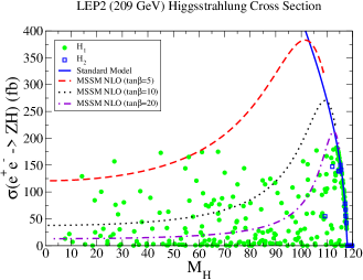
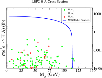
Figure 1: Cross sections at LEP2 (a) for $ZH_{i}$ production and (b) for $A_{i}H_{j}$ production versus the relevant Higgs boson mass. In (a), the solid curve is the SM production, and the dashed, dotted and dash-dotted are for the MSSM with $\tan\beta=5,10,20$, respectively. In (b), the curves is with $\tan\beta=5$.

We show the production cross sections at LEP2 versus the relevant Higgs boson mass parameter in Fig. 1 for (a) the $ZH_{i}$ channels and (b) $A_{i}H_{j}$ channels. Each symbol point indicates a solution satisfying all the constraints listed in this section. For comparison, the SM production rate is plotted by the solid curve in (a), and the dashed, dotted, and dash-dotted, are for the MSSM with $\tan\beta=5,10,20$, respectively. In (b), the curve is with $\tan\beta=5$. MSSM curves are at NLO using the software HPROD HPROD . It is interesting that there are solutions that have a CP-even Higgs as light as $M_{H_{1}}\approx 8$ GeV, and a CP-odd state $M_{A_{1}}\approx 6$ GeV, that satisfy the LEP2 bounds. After removing the solutions incompatible with the $ZH$ bound from LEP2, there are essentially no solutions that lead to sizable cross sections in the $AH$ channel, as seen in Fig. 1(b). The size of these masses reflects only the range of parameters we chose for scanning. As long as the light states are mostly singlet in composition, they can be arbitrarily light. As shown in Eq. (11) and Eq. (12), the $A_{1}$ can be tuned to be very light.

IV Mass Spectrum and Couplings for Higgs Bosons

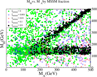
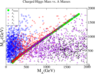
Figure 2: (a) $M_{H}-M_{A}$ mass plane, labeled according to MSSM fraction $\xi_{\rm MSSM}$. For each point both $H_{i}$ and $A_{i}$ satisfy the condition $\xi_{\rm MSSM}>0,0.001,0.01,0.1$, or $0.9$. All pairs $(M_{H_{i}},M_{A_{j}})$ are plotted. (b) $M_{H^{+}}-M_{A}$ mass plane with the MSSM $A^{\rm MSSM}$ mass $M^{\rm MSSM}_{A}=2A_{h}hv_{s}/\sin{2\beta}$ included for comparison.

We first point out the relaxed upper bound on the mass of the lightest CP-even Higgs boson. As given in Eq. (10), the lightest CP-even Higgs boson mass at tree level would vanish in the limit $h\to 0$, $g_{Z^{\prime}}\to 0$ and $\tan\beta\to 1$. Using the parameters discussed in III.1, the upper limit on the lightest Higgs boson mass at tree level as given by the first two terms in Eq. (10) is $142\,\mbox{GeV}$. Including the effects of Higgs mixing and the one-loop top correction, we find masses up to $\sim 168\,\mbox{GeV}$. The mass could be made even larger if we allowed $h>1$, although the perturbativity requirement up to the GUT scale at 1-loop level would imply that $h\leq 0.8$. We know that new heavy exotic matter must enter this model to cancel anomalies, so it is not necessarily justified to require $h$ to be perturbative to the Planck scale by calculating its 1-loop running using only low energy fields.

The masses of the various Higgs particles are a function of the mixing parameters, and most of the simple MSSM relations among masses are broken. It is quite common to have a light singlet with sizable MSSM fraction that can still evade the LEP2 bounds. Typical allowed light CP-even and odd masses are shown in Fig. 2(a) for various ranges of MSSM fractions. We see that it is possible to have light MSSM Higgs bosons below about 100 GeV without conflicting the LEP2 searches. This is because of the reduced couplings to the $Z$ when the MSSM fraction becomes small. One can clearly make out the usual MSSM structure when $\xi_{\rm MSSM}$ is large, with the diagonal band for $\xi_{\rm MSSM}>0.9$ being $M^{\rm MSSM}_{H}\simeq M^{\rm MSSM}_{A}$, and the horizontal band being the saturation of $M^{\rm MSSM}_{h}$ at its upper bound in the decoupling limit. As $\xi_{MSSM}$ decreases, we can see points in the lower left that are able to evade the LEP2 bounds on $M_{h,H}$ and $M_{A}$.

The mass range for the charged Higgs boson is demonstrated in Fig. 2(b). There is still a linear relationship between the charged Higgs mass and the MSSM $A$ mass since the singlets do not affect the $H^{+}$ mass. However, after mixing there is not necessarily a state with that mass, or the identity of the state is obscured. Most of the parameter space has a single state that can be identified as MSSM-like, with $\xi_{\rm MSSM}\sim 1$; in such circumstances there is also generally an $H$ very close in mass to both the $A$ and $H^{+}$. This is demonstrated in Appendix (A-3) with $M_{A_{3}}=774$, $M_{H^{+}}=792$, and $M_{H_{4}}=780$ GeV. However, the difference between $M_{H^{+}}$ and the $M_{A_{i}}$ can be 50 GeV or more due to mixing, especially when the MSSM-like state is not clearly identifiable. Such an example is presented in Appendix (A-5).

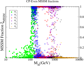
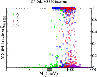
Figure 3: The MSSM fraction (a) for the CP-even and (b) for the CP-odd states.

The MSSM fractions are shown versus the masses of $H_{i}$ and $A_{i}$ in Fig. 3. It becomes more transparent that lighter Higgs bosons can be consistent with the LEP bound as long as the MSSM fraction is less than about 0.2. Another way to illustrate this is via the $ZZH$ coupling relative to its SM value, as shown in Fig. 4. We see that the LEP2 bound for $M_{H}>114$ GeV is restored only for those $H_{i}$ states in which the couplings to $Z$ become substantial. This figure is remarkably similar to Fig. 3 because the $ZZH$ coupling is $\sqrt{\xi_{\rm MSSM}}\cos(\alpha-\beta)\lambda_{\rm ZZH,SM}$ where $\alpha$ is the angle that diagonalizes the CP-even mass matrix in the MSSM.

One of the most important parameters in the SUSY Higgs sector is $\tan\beta$. In the model under consideration, $\tan\beta\approx 1$ is favored (because $A_{h}$ must be large enough to ensure $SU(2)$ breaking). We show the value of $\tan\beta$ versus the allowed ranges of masses of $H_{i}$ and $A_{i}$ in Fig. 5. Though the model naturally favors $\tan\beta\approx 1$, there are solutions deviating from this relation. The actual range reflects our parameter scanning methodology shown in Table 1, which results in $1/e<\tan\beta<e$.

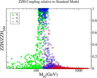
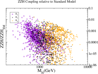
Figure 4: $ZZH$ coupling of the CP-even Higgs, relative to the Standard Model $ZZH$ coupling.

V Higgs Boson Decay and Production in $e^{+}e^{-}$ Collisions

Due to the rather distinctive features of the Higgs sector different from the SM and MSSM, it is important to study how the lightest Higgs bosons decay in order to explore their possible observation at future collider experiments. The lightest Higgs bosons can decay to quite non-standard channels, leading to distinctive, yet sometimes difficult experimental signatures. For the Higgs boson production and signal observation, we concentrate on an $e^{+}e^{-}$ linear collider. It is known that a linear collider can provide a clean experimental environment to sensitively search for and accurately study new physics signatures. If the Higgs bosons are discovered at the LHC, a linear collider would be needed to disentangle the complicated signals in this class of models. If, on the other hand, a Higgs boson is not observed at the LHC due to the decay modes difficult to observe at the hadron collider environment, a linear collider will serve as a discovery machine.

V.1 Lightest CP-Even State $H_{1}$

The main decay modes and corresponding branching fractions for the lightest CP-even Higgs $H_{1}$ are presented in Fig. 6. For lightest Higgs masses below approximately 100 GeV, the LEP2 constraint is very tight, and the lightest Higgs must be mostly singlet. Thus, the decay modes to $A_{1}A_{1}$ and $\chi^{0}_{1}\chi^{0}_{1}$ are dominant when they are kinematically allowed, due to the presence of the extra $U(1)^{\prime}$ gauge coupling and trilinear superpotential terms proportional to $h$ and $\lambda$. When those modes are not kinematically accessible, the decays are very similar to the MSSM modulo an eigenvector factor that is essentially how much of $H_{2}$ and $H_{1}$ are in the lightest state. Therefore $b\bar{b}$, $c\bar{c}$ and $\tau^{+}\tau^{-}$ decays dominate, with $c\bar{c}$ and $\tau^{+}\tau^{-}$ approximately an order of magnitude smaller than $b\bar{b}$, due to the difference in their Yukawa couplings. Examples of this kind can be seen in Appendices (A-3, A-5). Since $\tan\beta\approx 1$, the $c\bar{c}$ mode can be competitive with both $\tau^{+}\tau^{-}$ and $b\bar{b}$ since their masses are similar. In the MSSM the $c\bar{c}$ mode is suppressed because $\tan\beta$ is expected to be larger.

When the lightest Higgs is heavier than the LEP2 bound, it does not need to be mostly singlet, and there can be a continuum of branching ratios to $A_{1}A_{1}$, $\chi_{1}^{0}\chi_{1}^{0}$ or SM particles, depending on how much singlet is in the lightest state. This is indeed seen in Fig. 7 for a heavier $H_{1}$ where the modes $H_{1}\to W^{+}W^{-},\ ZZ$ become substantial.

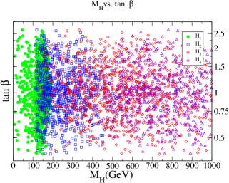
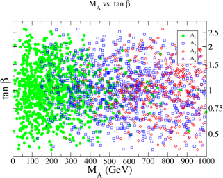
Figure 5: Range of $\tan\beta$ versus (a) the CP-even, and (b) CP-odd masses.

A striking feature of this graph is that the usual “discovery” modes for $M_{H_{1}}<140$, $H_{1}\rightarrow b\bar{b},\ \tau^{+}\tau^{-}$ are often strongly suppressed by decays to $A_{1}$ and $\chi^{0}_{1}$. Only $H_{1}\rightarrow W^{+}W^{-},\ ZZ$ decays are able to compete with the new $A_{1}$ and $\chi_{1}^{0}$ decays, which are all of gauge strength. A striking example of this is Appendix (A-6) and (A-7). One can see that the traditional shape of the $W^{+}W^{-}$ and $ZZ$ threshold is obscured by the presence of $\chi_{1}^{0}$ and $A$ decays, depending on what is kinematically accessible. For a $H_{1}$ heavy enough for these decay modes to be open, however, the coupling $h$ is typically greater than 0.8, large enough that it will become non-perturbative before the Planck scale unless new thresholds enter at a lower scale to modify its running. Such examples can be seen in Appendices (A-2, A-7, A-8).

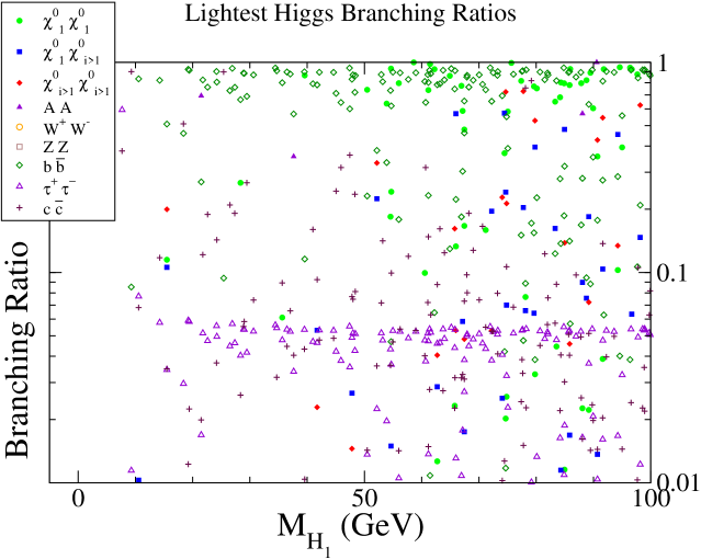
Figure 6: Branching ratios of the lightest CP-even Higgs in the low mass region $M_{H_{1}}<100$ GeV

The $A_{1}$ or $H_{1}$ can be lighter than the $\chi^{0}_{1}$. However, we assume R-parity is conserved. Therefore, decays of $\chi^{0}_{1}$ to $A_{1}$ or $H_{1}$ are not allowed and the lightest neutralino is assumed to be the (stable) LSP. We do not analyze the sfermion sector, which can produce a sfermion LSP in some regions of parameter space, but these scenarios are phenomenologically disfavored. We therefore assume $H$ and $A$ decays to $\chi^{0}_{1}$ are invisible at a collider. We separate the heavier neutralinos $\chi^{0}_{i>1}$ which may decay visibly neutralinodecays .

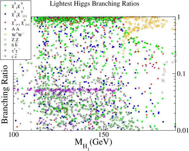
Figure 7: Branching ratios of the lightest CP-even Higgs in the high mass region $M_{H_{1}}>100$ GeV

V.2 CP-Odd

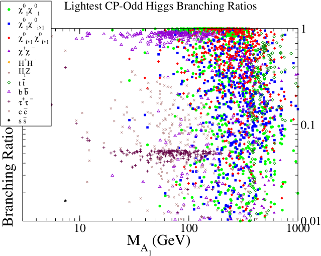
Figure 8: Branching ratios for the lightest CP-odd Higgs

The decays of the CP-odd Higgs bosons are presented in Fig. 8. The light $A_{1}$ will decay dominantly to neutralinos when it is kinematically possible. When it is not, it decays dominantly into the nearest mass SM fermion, which is usually $b$ unless the $A_{1}$ is lighter than the $b\bar{b}$ pair mass. Charm and tau decays can also be significant, depending on the value of $\tan\beta$. The $c\bar{c}$ decays are about 3 times more likely than the $\tau^{+}\tau^{-}$ due to the color factor. However, for larger $\tan\beta$ the $\tau^{+}\tau^{-}$ dominates.

For heavy $A_{1}\mathrel{\raise 1.29167pt\hbox{$>$\kern-7.5pt\lower 4.30554pt\hbox{$\sim$}}}200$ GeV, decays to neutralinos and charginos universally dominate due to their gauge strength, suppressing the $b\bar{b}$ mode below 10%.

The lightest $A$ can decay only into light SM fermions, the photon, and neutralinos. Hadronic bottom and charm decays are difficult to separate from background, and $\tau$’s are obscured by missing energy and hadronic background.

V.3 The Higgs signatures at a linear collider

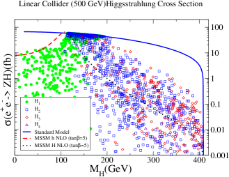
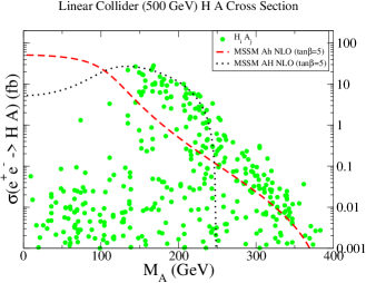
Figure 9: Cross section at a 500  GeV linear collider (a) for $ZH_{i}$ production, and (b) for $A_{i}H_{j}$ production versus the corresponding Higgs boson mass. In (a), the solid curve is the SM production, and the dashed and dot-dashed for MSSM $h$ and $H$ production with $\tan\beta=5$.

The production via radiation of a Higgs from a virtual $Z$ boson is the dominant mechanism for CP-even Higgs production at a linear collider. We show this cross section in Fig. 9, where each point is a viable model solution satisfying all the constraints. The curves present the SM and MSSM cross sections for comparison. Model points with $M_{H}<114.1$ are only those with suppressed coupling to the $Z$, and those with large MSSM fraction are removed by the LEP2 bounds discussed in Section III.4. As can be seen from Eq. (18) the ratio between the Standard Model cross section and that for any model point simply reflects the amount of mixing into the SM-like or MSSM-like Higgs for a given Higgs state. Since this ratio comes entirely from the $HZZ$ vertex, Fig. 9(a) and Fig. 10 are just Fig. 4 times the SM curve, as given in Eq. (18).

The production cross sections for the heavier Higgs particles are very small. One can see the coupling to $ZZH$ in Fig. 4. For heavy states (that correspond to the $H$ in MSSM), $\cos(\alpha-\beta)\rightarrow 0$ as the $H$ gets heavier. In this decoupling limit of the MSSM the heavy $H$ has no coupling to the $Z$.

In supersymmetric models if both the $A$ and $H$ are light enough they can be produced by the process $e^{+}e^{-}\rightarrow HA$ at a lepton collider. We present this cross section in Fig. 9(b). In this model the $HA$ cross sections do not provide additional constraint, and few model points are removed, unlike the $HZ$ cross sections. The $HA$ cross section is normally much smaller than the $HZ$ cross section unless the center of mass energy is above and close to $M_{H}+M_{A}$. As can be seen in Fig. 9(b), the cross section is largest in this channel when $M_{A}\simeq M_{H}\simeq\sqrt{s}/2$, and they have large $\xi_{\rm MSSM}$. This is confirmed by seeing the MSSM curves as shown in Fig. 9(b).

At 500 GeV the weak boson fusion production modes $e^{+}e^{-}\rightarrow\nu\bar{\nu}H,\ e^{+}e^{-}H$ as shown in Fig. 10 are comparable in size to the Higgsstrahlung mode. At higher energies, the weak boson fusion becomes larger than Higgsstrahlung and is the most important production mode. These curves are similar to Fig. 9(a), reflecting that all of these single Higgs production modes are simply a mixing factor times the Standard Model curve. It is particularly interesting to note that the $ZZ$ fusion channel $e^{+}e^{-}\to e^{+}e^{-}H$ can serve as a model-independent process to measure the $ZZH$ coupling regardless the decay of $H$, even if $H$ is invisible Gunion:1998jc .

As anticipated for the next generation linear collider with $\sqrt{s}=500$ GeV and an integrated luminosity of the order of $500-1000$ fb^-1, one should be able to cover a substantial region of the parameter space. For instance, with a cross section of the order of 0.1 fb, this may lead to about 50$-$100 events. As for further exploration of signal searches, it depends on specific model parameters. While we have provided a comprehensive list of representative models in the Appendices, we discuss a few of them for the purpose of illustration.

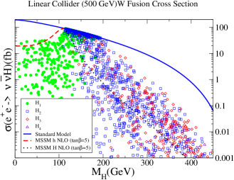
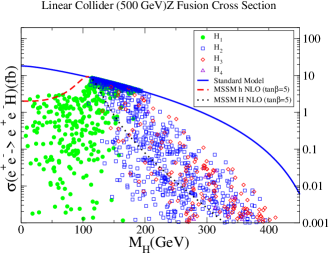
Figure 10: Cross section at a 500  GeV linear collider for $H_{i}$ production in (a) $WW$ fusion, and (b) $ZZ$ fusion versus the corresponding Higgs boson mass. The solid curves are the SM production, and the dashed and dot-dashed for MSSM $h$ and $H$ production with $\tan\beta=5$. In both graphs, interference from the $Z\rightarrow\nu\overline{\nu}$ and $Z\rightarrow e^{+}e^{-}$ decays are neglected.

• MSSM-like: Examples of this type are presented in Appendices (A-9,  A-3, A-10, A-5, A-11). When the MSSM fractions are close to one, the model is MSSM-like and their mass relations approximately hold. The standard MSSM or SM discovery modes are present for the lightest CP-even state, even if with reduced rates. As long as the Higgs boson mass is not nearly degenerate with $M_{Z}$, the signal observation should be quite feasible at the LC, as well as at the LHC.

• $H\rightarrow$ multi-jets: Examples of this type are presented in Appendices (A-1,  A-7). Certain parameters may lead to the dominant decay modes $H_{i}\rightarrow H_{j}H_{j}$ or $H_{i}\rightarrow A_{j}A_{j}$ with the $H_{j}$ or $A_{j}$ decaying hadronically, or to $\tau$’s. This scenario would make the signal search nearly impossible at hadron colliders due to the overwhelming QCD backgrounds. This is the typical difficult scenario studied for the NMSSM nmssmpheno . At a LC, however, the reconstruction of the Higgs mass peak from jets is still possible. In particular, if the Higgsstrahlung process yields a sizable cross section, the signal could be picked up from the recoiled mass against the distinctive signature of $Z\to e^{+}e^{-},\mu^{+}\mu^{-}$.

• Invisible: Examples of this type are presented in Appendices (A-6, A-8, A-12). MSSM and SM detection modes are heavily suppressed by $H_{i}\rightarrow\chi^{0}\chi^{0},A_{j}A_{j},H_{j}H_{j}$ and dominant decays eventually produce neutralinos. It is possible to discover a Higgs in this mode at the LHC if its cross section is large enough Cavalli:2002vs . At an $e^{+}e^{-}$ linear collider on the other hand, the Higgsstrahlung process with $Z\to\ell^{+}\ell^{-}$ and the $ZZ$ fusion process may yield a sizable cross section and can make accurate measurements of this invisible decay channel by detecting the recoiling $\ell^{+}\ell^{-}$ plus large missing energy.

• Neutralino: Examples of this type are presented in the Appendices (all appendices have an example of this type). One or more Higgs decays into heavy neutralinos, which can then decay via cascade to the LSP, producing visible signals and large missing energy neutralinodecays . If the lightest neutralino is mostly singlino or $Z^{\prime}$-ino, the usual MSSM limits on neutralino mass do not apply, and couplings between it and Higgs bosons can be large. This mode is extremely important, and dominates the Higgs decays due to the presence of Higgs-singlet interaction $h$, singlet-singlet interactions $\lambda$ and the $Z^{\prime}$ coupling. This mode has received some attention in the literature singlinopheno but clearly warrants more due to its dominance in parameter space.

It is clear that the model studied in this paper presents very rich physics in the Higgs sector. An $e^{+}e^{-}$ linear collider will be ideally suited for the detailed exploration of the non-standard Higgs physics. Analyses for the LHC should also be performed, particularly for the non-MSSM modes nmssmpheno .

VI Summary and Conclusions

We have considered the Higgs sector in an extension of the MSSM with extra SM singlets. By exploiting an extra $U(1)^{\prime}$ gauge symmetry, the domain-wall problem is avoided. An effective $\mu$ parameter can be generated by a singlet VEV, which can be decoupled from the new gauge boson $Z^{\prime}$ mass.

The model involves a rich Higgs structure very different from that of the MSSM. In particular, there are large mixings between Higgs doublets and SM singlets. The lightest CP even Higgs boson can have a mass up to about 170 GeV. Higgs bosons considerably lighter than the LEP2 bound are allowed. The parameter $\tan\beta\sim 1$ is both allowed and theoretically favored.

We parameterize the Higgs coupling strengths relative to the MSSM, called the MSSM fraction $\xi_{\rm MSSM}$. We find that besides the typical SM-like and MSSM-like Higgs bosons, there are model points leading to very different signatures from those. One of the features for the Higgs boson decay is to have possibly a large invisible decay mode to LSP. We present a comprehensive list of model scenarios in the Appendices.

Concentrating on a future $e^{+}e^{-}$ linear collider with $\sqrt{s}=500$ GeV, we found that in a large parameter region the Higgs bosons are accessible through the production channels $e^{+}e^{-}\to ZH_{i},\ H_{i}A_{j}$ as well as $WW$ and $ZZ$ fusion. We outlined the searching strategy for some representative scenarios at a future linear collider.

We find that this model has a large parameter space where the Higgs bosons decay hadronically or invisibly. As these modes are very difficult at the LHC, effort should be invested in ways to discover or exclude such modes at the LHC. If discovery is not possible, a linear collider will absolutely be required.

We emphasize the importance of neutralino decays, which dominate the parameter space due to Higgs self-interactions and the $U(1)^{\prime}$ gauge coupling. These decays are generically present and dominant in extended models singlinopheno , and thus should be paid more attention by phenomenologists and experimentalists.

Acknowledgments
We thank V. Barger, J. Erler, J. Gunion, T. Li, and J. Wells, for useful discussions. This work was supported in part by DOE grants DE–FG02–95ER–40896, DE–FG03–91ER–40674 and DOE–EY–76–02–3071; also in part by the Wisconsin Alumni Research Foundation, the National Natural Science Foundation of China, the Davis Institute for High Energy Physics, and the U.C. Davis Dean’s office.

A-1 Lightest $A_{1}$

$\tan{\beta}=0.522$		$M_{Z^{\prime}}=2415$ GeV		$M_{H^{+}}=826$ GeV		$\alpha_{ZZ^{\prime}}=$-$2.7\!\cdot\!10^{-4}$
$M_{H}$	118	654	843	1731	2330	7839
$\xi_{\rm MSSM}$	1	$1.2\!\cdot\!10^{-3}$	1	$3.3\!\cdot\!10^{-3}$	$2.4\!\cdot\!10^{-4}$	0
$\sigma(H_{i}Z)$	58
$\sigma(H_{i}\nu\overline{\nu})$	87
$\sigma(H_{i}e^{+}e^{-})$	8.3
$M_{A}$	6	821	1741	7839	0	0
$\xi_{\rm MSSM}$	$3.2\!\cdot\!10^{-4}$	0.99	$5.9\!\cdot\!10^{-3}$	0	1	$5.4\!\cdot\!10^{-4}$
$\sigma(H_{1}A)$	$4.8\!\cdot\!10^{-6}$
$M_{\chi^{0}}$	42	165	213	284	470	774	778	1834	3222
$\xi_{\rm MSSM}$	0.24	0.95	0.81	1	1	0	$2.1\!\cdot\!10^{-5}$	$9.7\!\cdot\!10^{-5}$	$4.5\!\cdot\!10^{-5}$
$\xi_{\tilde{s}}$	0.76	0.047	0.19	$1.1\!\cdot\!10^{-3}$	$9.2\!\cdot\!10^{-5}$	0.99	0.99	0.65	0.37
$\xi_{\tilde{Z^{\prime}}}$	0	0	0	0	0	$5.3\!\cdot\!10^{-3}$	0.012	0.35	0.63
$M_{\chi^{+}}$	173	470

Cross sections quoted are in fb for a linear $e^{+}e^{-}$ collider at center-of-mass energy 500 GeV.

$$v_{2}=80\,\mbox{GeV} v_{1}=154\,\mbox{GeV} v_{s}=272\,\mbox{GeV}$$

$$v_{s1}=117\,\mbox{GeV} v_{s2}=3504\,\mbox{GeV} v_{s3}=3256\,\mbox{GeV}$$

$$m_{H_{u}}^{2}=(849\,\mbox{GeV})^{2} m_{H_{d}}^{2}=(595\,\mbox{GeV})^{2} m_{S}^{2}=(1585\,\mbox{GeV})^{2}$$

$$m_{S_{1}}^{2}=(7817\,\mbox{GeV})^{2} m_{S_{2}}^{2}=(496\,\mbox{GeV})^{2} m_{S_{3}}^{2}=-(1115\,\mbox{GeV})^{2}$$

$$h=0.608 A_{h}=1704\,\mbox{GeV} \mu=hv_{s}=166\,\mbox{GeV}$$

$$\lambda=0.173 A_{\lambda}=3622\,\mbox{GeV}$$

$$M_{1}=-267\,\mbox{GeV} M_{1}^{\prime}=1385\,\mbox{GeV} M_{2}=459\,\mbox{GeV}$$

$$m_{SS_{1}}^{2}=-(48\,\mbox{GeV})^{2} m_{SS_{2}}^{2}=-(479\,\mbox{GeV})^{2}$$

Branching Ratios for dominant decay modes (greater than 1% excluding model-dependent squark, slepton, $Z^{\prime}$ and exotic decays; $\chi^{0}_{i>1}$ are summed):

$H_{1}$	$A_{1}A_{1}$	81%	$\chi^{0}_{1}\chi^{0}_{1}$	18%	$b\bar{b}$	1%
$H_{2}$	$\chi^{+}_{1}\chi^{-}_{1}$	25%	$\chi^{0}_{1}\chi^{0}_{i>1}$	17%	$W^{+}W^{-}$	14%	$\chi^{0}_{i>1}\chi^{0}_{i>1}$	14%	$t\bar{t}$	13%	$H_{1}H_{1}$	11%
$H_{3}$	$t\bar{t}$	77%	$\chi^{0}_{i>1}\chi^{0}_{i>1}$	8%	$\chi^{0}_{1}\chi^{0}_{i>1}$	8%	$\chi^{0}_{1}\chi^{0}_{1}$	3%	$\chi^{+}_{1}\chi^{-}_{2}$	2%	$H_{1}H_{1}$	1%
$H_{4}$	$A_{1}A_{2}$	27%	$\chi^{+}_{1}\chi^{-}_{1}$	23%	$\chi^{0}_{i>1}\chi^{0}_{i>1}$	18%	$H_{1}H_{3}$	7%	$\chi^{0}_{1}\chi^{0}_{i>1}$	6%	$W^{+}W^{-}$	4%
$H_{5}$	$W^{+}W^{-}$	24%	$H_{1}H_{1}$	24%	$ZZ$	12%	$H_{2}H_{2}$	9%	$\chi^{0}_{i>1}\chi^{0}_{i>1}$	7%	$\chi^{+}_{1}\chi^{-}_{1}$	6%
$H_{6}$	$\chi^{0}_{i>1}\chi^{0}_{i>1}$	95%	$H_{2}H_{5}$	3%	$H_{2}H_{2}$	1%
$A_{1}$	$c\bar{c}$	83%	$\tau^{+}\tau^{-}$	16%	$s\bar{s}$	1%
$A_{2}$	$t\bar{t}$	79%	$\chi^{0}_{i>1}\chi^{0}_{i>1}$	9%	$\chi^{0}_{1}\chi^{0}_{1}$	6%	$\chi^{0}_{1},\chi^{0}_{i>1}$	5%	$\chi^{+}_{1}\chi^{-}_{1}$	1%
$A_{3}$	$H_{2}Z$	97%	$\chi^{+}_{1}\chi^{-}_{1}$	1%	$\chi^{0}_{i>1}\chi^{0}_{i>1}$	1%
$A_{4}$	$H_{2}Z$	64%	$H_{5}Z$	31%	$\chi^{0}_{i>1}\chi^{0}_{i>1}$	3%	$A_{1}H_{2}$	1%

Eigenvectors/rotation matrices

$$R_{H}=\left[\begin{array}[]{cccccc}\scriptstyle 0.45&\scriptstyle 0.89&\scriptstyle 0.038&\scriptstyle 0.00063&\scriptstyle 0.0045&\scriptstyle 0.014\\ \vskip 6.0pt plus 2.0pt minus 2.0pt\cr\scriptstyle 0.022&\scriptstyle\scriptstyle-0.026&\scriptstyle\scriptstyle 0.086&\scriptstyle\scriptstyle 0.045&\scriptstyle\scriptstyle 0.90&\scriptstyle\scriptstyle 0.42\\ \vskip 6.0pt plus 2.0pt minus 2.0pt\cr\scriptstyle 0.89&\scriptstyle-0.45&\scriptstyle 0.043&\scriptstyle-0.0016&\scriptstyle-0.031&\scriptstyle-0.017\\ \vskip 6.0pt plus 2.0pt minus 2.0pt\cr\scriptstyle 0.056&\scriptstyle 0.011&\scriptstyle-0.99&\scriptstyle 0.0066&\scriptstyle 0.023&\scriptstyle 0.15\\ \vskip 6.0pt plus 2.0pt minus 2.0pt\cr\scriptstyle 0.0096&\scriptstyle 0.012&\scriptstyle-0.13&\scriptstyle-0.021&\scriptstyle 0.42&\scriptstyle-0.90\\ \vskip 6.0pt plus 2.0pt minus 2.0pt\cr\scriptstyle-0.000018&\scriptstyle-0.000034&\scriptstyle 0.000043&\scriptstyle-1.0&\scriptstyle 0.032&\scriptstyle 0.039\end{array}\right]$$

$$R_{A}=\left[\begin{array}[]{cccccc}\scriptstyle-0.016&\scriptstyle-0.0083&\scriptstyle 0.068&\scriptstyle 0.046&\scriptstyle-0.88&\scriptstyle-0.47\\ \vskip 6.0pt plus 2.0pt minus 2.0pt\cr\scriptstyle 0.88&\scriptstyle\scriptstyle 0.46&\scriptstyle\scriptstyle-0.075&\scriptstyle\scriptstyle 0.00088&\scriptstyle\scriptstyle-0.026&\scriptstyle\scriptstyle 0.000040\\ \vskip 6.0pt plus 2.0pt minus 2.0pt\cr\scriptstyle-0.068&\scriptstyle\scriptstyle-0.035&\scriptstyle\scriptstyle-0.99&\scriptstyle\scriptstyle 0.0027&\scriptstyle\scriptstyle-0.076&\scriptstyle\scriptstyle 0.00012\\ \vskip 6.0pt plus 2.0pt minus 2.0pt\cr\scriptstyle 0.00000045&\scriptstyle\scriptstyle 0.00000023&\scriptstyle\scriptstyle 0.00017&\scriptstyle\scriptstyle 1.0&\scriptstyle\scriptstyle 0.033&\scriptstyle\scriptstyle 0.036\\ \vskip 6.0pt plus 2.0pt minus 2.0pt\cr\scriptstyle 0.46&\scriptstyle\scriptstyle-0.89&\scriptstyle\scriptstyle 0.00078&\scriptstyle\scriptstyle-0.00033&\scriptstyle\scriptstyle-0.010&\scriptstyle\scriptstyle 0.019\\ \vskip 6.0pt plus 2.0pt minus 2.0pt\cr\scriptstyle 0.018&\scriptstyle\scriptstyle-0.014&\scriptstyle\scriptstyle-0.037&\scriptstyle\scriptstyle 0.016&\scriptstyle\scriptstyle 0.47&\scriptstyle\scriptstyle-0.88\end{array}\right]$$

$$R_{\chi^{0}}=\left[\begin{array}[]{ccccccccc}\scriptstyle-0.0011&\scriptstyle 0.064&\scriptstyle 0.053&\scriptstyle-0.45&\scriptstyle-0.15&\scriptstyle\scriptstyle 0.87&\scriptstyle\scriptstyle 0.00096&\scriptstyle\scriptstyle 0.030&\scriptstyle\scriptstyle-0.028\\ \vskip 6.0pt plus 2.0pt minus 2.0pt\cr\scriptstyle-0.00051&\scriptstyle\scriptstyle-0.36&\scriptstyle\scriptstyle-0.11&\scriptstyle\scriptstyle 0.58&\scriptstyle\scriptstyle-0.69&\scriptstyle\scriptstyle 0.22&\scriptstyle\scriptstyle 0.00048&\scriptstyle\scriptstyle 0.0046&\scriptstyle\scriptstyle-0.0042\\ \vskip 6.0pt plus 2.0pt minus 2.0pt\cr\scriptstyle 0.00052&\scriptstyle-0.020&\scriptstyle-0.072&\scriptstyle 0.60&\scriptstyle 0.67&\scriptstyle 0.43&\scriptstyle-0.00055&\scriptstyle 0.0046&\scriptstyle-0.0041\\ \vskip 6.0pt plus 2.0pt minus 2.0pt\cr\scriptstyle 0.000051&\scriptstyle 0.93&\scriptstyle-0.038&\scriptstyle 0.27&\scriptstyle-0.24&\scriptstyle 0.033&\scriptstyle-0.000052&\scriptstyle\scriptstyle-0.00029&\scriptstyle\scriptstyle 0.00025\\ \vskip 6.0pt plus 2.0pt minus 2.0pt\cr\scriptstyle 0.00020&\scriptstyle\scriptstyle 0.0082&\scriptstyle\scriptstyle-0.99&\scriptstyle-0.14&\scriptstyle 0.027&\scriptstyle-0.0095&\scriptstyle-0.00030&\scriptstyle 0.00087&\scriptstyle-0.00057\\ \vskip 6.0pt plus 2.0pt minus 2.0pt\cr\scriptstyle-0.073&\scriptstyle 0.000063&\scriptstyle-0.00038&\scriptstyle-0.0020&\scriptstyle-0.00066&\scriptstyle 0.0081&\scriptstyle\scriptstyle 0.71&\scriptstyle\scriptstyle-0.61&\scriptstyle\scriptstyle-0.34\\ \vskip 6.0pt plus 2.0pt minus 2.0pt\cr\scriptstyle-0.11&\scriptstyle\scriptstyle 0.00019&\scriptstyle\scriptstyle-0.00014&\scriptstyle\scriptstyle 0.0038&\scriptstyle\scriptstyle 0.0026&\scriptstyle\scriptstyle-0.013&\scriptstyle\scriptstyle 0.69&\scriptstyle\scriptstyle 0.67&\scriptstyle\scriptstyle 0.26\\ \vskip 6.0pt plus 2.0pt minus 2.0pt\cr\scriptstyle 0.59&\scriptstyle-0.00015&\scriptstyle 0.00018&\scriptstyle-0.0085&\scriptstyle-0.0050&\scriptstyle 0.029&\scriptstyle 0.13&\scriptstyle-0.32&\scriptstyle 0.73\\ \vskip 6.0pt plus 2.0pt minus 2.0pt\cr\scriptstyle-0.79&\scriptstyle 0.000050&\scriptstyle-0.00012&\scriptstyle-0.0060&\scriptstyle-0.0029&\scriptstyle 0.022&\scriptstyle-0.063&\scriptstyle-0.27&\scriptstyle 0.54\end{array}\right]$$

$$R_{\chi^{+}}=\left[\begin{array}[]{cccc}\scriptstyle 0.027&\scriptstyle-0.71&\scriptstyle-0.14&\scriptstyle 0.69\\ \vskip 6.0pt plus 2.0pt minus 2.0pt\cr\scriptstyle 0.027&\scriptstyle-0.71&\scriptstyle 0.14&\scriptstyle-0.69\\ \vskip 6.0pt plus 2.0pt minus 2.0pt\cr\scriptstyle 0.71&\scriptstyle\scriptstyle 0.027&\scriptstyle\scriptstyle-0.69&\scriptstyle\scriptstyle-0.14\\ \vskip 6.0pt plus 2.0pt minus 2.0pt\cr\scriptstyle 0.71&\scriptstyle\scriptstyle 0.027&\scriptstyle\scriptstyle 0.69&\scriptstyle\scriptstyle 0.14\end{array}\right]$$

where $H_{i}^{\rm mass}=R_{H}\Re H^{\rm gauge},A_{i}^{\rm mass}=R_{A}\Im H^{\rm gauge}$ with $H^{\rm gauge}=[H_{1}^{0},H_{2}^{0},S,S_{1},S_{2},S_{3}]^{T}$; $A_{5}$ and $A_{6}$ are goldstone bosons corresponding to the $Z$ and $Z^{\prime}$. $\chi^{0}_{\rm mass}=R_{\chi^{0}}[\tilde{Z}^{\prime},\tilde{B},\tilde{W}^{0},\tilde{H}_{2}^{0},\tilde{H}_{1}^{0},\tilde{S},\tilde{S}_{1},\tilde{S}_{2},\tilde{S}_{3}]^{T}$, and $\chi^{+}_{\rm mass}=R_{\chi^{+}}[\tilde{W}^{+},\tilde{H}_{1}^{+},\tilde{W}^{-},\tilde{H}_{2}^{-}]^{T}$.

A-2 Lightest $H_{1}$

$\tan{\beta}=0.614$		$M_{Z^{\prime}}=626$ GeV		$M_{H^{+}}=444$ GeV		$\alpha_{ZZ^{\prime}}=$-$3.3\!\cdot\!10^{-3}$
$M_{H}$	8	127	471	627	1071	1762
$\xi_{\rm MSSM}$	0.013	0.99	1	$1.4\!\cdot\!10^{-3}$	$4.5\!\cdot\!10^{-5}$	$3.6\!\cdot\!10^{-4}$
$\sigma(H_{i}Z)$	0.86	55
$\sigma(H_{i}\nu\overline{\nu})$	2.5	78	$3.5\!\cdot\!10^{-5}$
$\sigma(H_{i}e^{+}e^{-})$	0.23	7.5	$3.2\!\cdot\!10^{-6}$
$M_{A}$	172	446	1067	1757	0	0
$\xi_{\rm MSSM}$	$2.0\!\cdot\!10^{-4}$	1	$1.4\!\cdot\!10^{-4}$	$6.2\!\cdot\!10^{-4}$	1	$1.7\!\cdot\!10^{-3}$
$\sigma(H_{1}A)$	$1.1\!\cdot\!10^{-7}$	$6.8\!\cdot\!10^{-6}$
$\sigma(H_{2}A)$	$2.3\!\cdot\!10^{-5}$
$M_{\chi^{0}}$	44	47	58	62	120	170	286	556	1357
$\xi_{\rm MSSM}$	0.98	0.3	$2.3\!\cdot\!10^{-4}$	$4.4\!\cdot\!10^{-4}$	0.94	0.77	$3.2\!\cdot\!10^{-3}$	1	$3.1\!\cdot\!10^{-4}$
$\xi_{\tilde{s}}$	0.015	0.7	1	1	0.059	0.23	0.82	0	0.18
$\xi_{\tilde{Z^{\prime}}}$	0	$1.2\!\cdot\!10^{-4}$	$3.4\!\cdot\!10^{-4}$	$5.3\!\cdot\!10^{-5}$	$4.7\!\cdot\!10^{-5}$	0	0.18	0	0.82
$M_{\chi^{+}}$	103	556

Cross sections quoted are in fb for a linear $e^{+}e^{-}$ collider at center-of-mass energy 500 GeV.

$$v_{2}=91\,\mbox{GeV} v_{1}=148\,\mbox{GeV} v_{s}=212\,\mbox{GeV}$$

$$v_{s1}=1726\,\mbox{GeV} v_{s2}=120\,\mbox{GeV} v_{s3}=397\,\mbox{GeV}$$

$$m_{H_{u}}^{2}=(194\,\mbox{GeV})^{2} m_{H_{d}}^{2}=-(184\,\mbox{GeV})^{2} m_{S}^{2}=(1770\,\mbox{GeV})^{2}$$

$$m_{S_{1}}^{2}=-(310\,\mbox{GeV})^{2} m_{S_{2}}^{2}=(1001\,\mbox{GeV})^{2} m_{S_{3}}^{2}=(580\,\mbox{GeV})^{2}$$

$$h=-0.552 A_{h}=764\,\mbox{GeV} \mu=hv_{s}=-117\,\mbox{GeV}$$

$$\lambda=0.035 A_{\lambda}=3234\,\mbox{GeV}$$

$$M_{1}=-31\,\mbox{GeV} M_{1}^{\prime}=-1067\,\mbox{GeV} M_{2}=542\,\mbox{GeV}$$

$$m_{SS_{1}}^{2}=-(587\,\mbox{GeV})^{2} m_{SS_{2}}^{2}=-(536\,\mbox{GeV})^{2}$$

Branching Ratios for dominant decay modes (greater than 1% excluding model-dependent squark, slepton, $Z^{\prime}$ and exotic decays; $\chi^{0}_{i>1}$ are summed):

$H_{1}$	$\tau^{+}\tau^{-}$	59%	$c\bar{c}$	38%	$s\bar{s}$	2%
$H_{2}$	$\chi^{0}_{i>1}\chi^{0}_{i>1}$	60%	$\chi^{0}_{1}\chi^{0}_{i>1}$	17%	$\chi^{0}_{1}\chi^{0}_{1}$	13%	$H_{1}H_{1}$	6%	$b\bar{b}$	4%
$H_{3}$	$t\bar{t}$	66%	$\chi^{0}_{i>1}\chi^{0}_{i>1}$	20%	$\chi^{0}_{1}\chi^{0}_{i>1}$	8%	$H_{2}H_{2}$	4%	$W^{+}W^{-}$	1%	$ZZ$	1%
$H_{4}$	$A_{1}A_{1}$	41%	$H_{1}H_{1}$	35%	$\chi^{0}_{i>1}\chi^{0}_{i>1}$	12%	$H_{2}H_{2}$	3%	$W^{+}W^{-}$	3%	$\chi^{+}_{1}\chi^{-}_{1}$	2%
$H_{5}$	$\chi^{0}_{i>1}\chi^{0}_{i>1}$	59%	$\chi^{+}_{1}\chi^{-}_{1}$	13%	$H_{1}H_{1}$	8%	$A_{1}A_{1}$	4%	$A_{2}A_{2}$	4%	$H_{1}H_{4}$	3%
$H_{6}$	$\chi^{0}_{i>1}\chi^{0}_{i>1}$	41%	$\chi^{+}_{1}\chi^{-}_{1}$	38%	$A_{2}A_{2}$	5%	$H_{3}H_{3}$	4%	$\chi^{0}_{1}\chi^{0}_{i>1}$	3%	$H_{2}H_{3}$	2%
$A_{1}$	$\chi^{0}_{i>1}\chi^{0}_{i>1}$	98%	$\chi^{0}_{1}\chi^{0}_{1}$	2%	$\chi^{0}_{1},\chi^{0}_{i>1}$	1%
$A_{2}$	$t\bar{t}$	62%	$\chi^{0}_{i>1}\chi^{0}_{i>1}$	26%	$\chi^{0}_{1},\chi^{0}_{i>1}$	7%	$\chi^{+}_{1}\chi^{-}_{1}$	2%	$H_{2}Z$	1%	$\chi^{0}_{1}\chi^{0}_{1}$	1%
$A_{3}$	$H_{2}Z$	100%
$A_{4}$	$\chi^{0}_{i>1}\chi^{0}_{i>1}$	44%	$\chi^{+}_{1}\chi^{-}_{1}$	41%	$H_{2}Z$	4%	$A_{1}H_{1}$	3%	$\chi^{0}_{1},\chi^{0}_{i>1}$	3%	$H_{5}Z$	2%

Eigenvectors/rotation matrices

$$R_{H}=\left[\begin{array}[]{cccccc}\scriptstyle 0.062&\scriptstyle 0.094&\scriptstyle 0.072&\scriptstyle 0.46&\scriptstyle 0.18&\scriptstyle 0.86\\ \vskip 6.0pt plus 2.0pt minus 2.0pt\cr\scriptstyle 0.46&\scriptstyle 0.88&\scriptstyle 0.0025&\scriptstyle-0.082&\scriptstyle-0.017&\scriptstyle-0.083\\ \vskip 6.0pt plus 2.0pt minus 2.0pt\cr\scriptstyle-0.88&\scriptstyle 0.47&\scriptstyle-0.015&\scriptstyle-0.010&\scriptstyle-0.00038&\scriptstyle 0.020\\ \vskip 6.0pt plus 2.0pt minus 2.0pt\cr\scriptstyle-0.0028&\scriptstyle 0.037&\scriptstyle 0.13&\scriptstyle 0.87&\scriptstyle-0.052&\scriptstyle-0.47\\ \vskip 6.0pt plus 2.0pt minus 2.0pt\cr\scriptstyle-0.0067&\scriptstyle-0.0011&\scriptstyle 0.14&\scriptstyle-0.060&\scriptstyle 0.97&\scriptstyle-0.18\\ \vskip 6.0pt plus 2.0pt minus 2.0pt\cr\scriptstyle-0.018&\scriptstyle-0.0070&\scriptstyle 0.98&\scriptstyle-0.14&\scriptstyle-0.15&\scriptstyle 0.023\end{array}\right]$$

$$R_{A}=\left[\begin{array}[]{cccccc}\scriptstyle 0.012&\scriptstyle 0.0074&\scriptstyle-0.033&\scriptstyle 0.42&\scriptstyle-0.16&\scriptstyle 0.89\\ \vskip 6.0pt plus 2.0pt minus 2.0pt\cr\scriptstyle 0.85&\scriptstyle\scriptstyle 0.52&\scriptstyle\scriptstyle-0.021&\scriptstyle\scriptstyle-0.045&\scriptstyle\scriptstyle 0.0074&\scriptstyle\scriptstyle 0.0058\\ \vskip 6.0pt plus 2.0pt minus 2.0pt\cr\scriptstyle-0.0099&\scriptstyle-0.0061&\scriptstyle-0.15&\scriptstyle-0.0052&\scriptstyle 0.97&\scriptstyle 0.17\\ \vskip 6.0pt plus 2.0pt minus 2.0pt\cr\scriptstyle 0.021&\scriptstyle 0.013&\scriptstyle 0.98&\scriptstyle 0.11&\scriptstyle 0.15&\scriptstyle 0.010\\ \vskip 6.0pt plus 2.0pt minus 2.0pt\cr\scriptstyle 0.52&\scriptstyle-0.85&\scriptstyle-0.00057&\scriptstyle 0.0047&\scriptstyle 0.00032&\scriptstyle-0.0021\\ \vskip 6.0pt plus 2.0pt minus 2.0pt\cr\scriptstyle 0.032&\scriptstyle 0.026&\scriptstyle-0.11&\scriptstyle 0.90&\scriptstyle 0.063&\scriptstyle-0.41\end{array}\right]$$

$$R_{\chi^{0}}=\left[\begin{array}[]{ccccccccc}\scriptstyle 0.0012&\scriptstyle 0.95&\scriptstyle-0.039&\scriptstyle 0.21&\scriptstyle-0.20&\scriptstyle-0.12&\scriptstyle\scriptstyle-0.019&\scriptstyle\scriptstyle 0.0091&\scriptstyle\scriptstyle-0.0033\\ \vskip 6.0pt plus 2.0pt minus 2.0pt\cr\scriptstyle 0.011&\scriptstyle\scriptstyle 0.18&\scriptstyle\scriptstyle 0.051&\scriptstyle\scriptstyle-0.48&\scriptstyle\scriptstyle-0.18&\scriptstyle\scriptstyle 0.82&\scriptstyle\scriptstyle 0.14&\scriptstyle\scriptstyle 0.021&\scriptstyle\scriptstyle-0.022\\ \vskip 6.0pt plus 2.0pt minus 2.0pt\cr\scriptstyle-0.019&\scriptstyle\scriptstyle 0.012&\scriptstyle-0.00096&\scriptstyle 0.0093&\scriptstyle 0.0016&\scriptstyle-0.012&\scriptstyle 0.30&\scriptstyle-0.71&\scriptstyle 0.63\\ \vskip 6.0pt plus 2.0pt minus 2.0pt\cr\scriptstyle-0.0073&\scriptstyle 0.0064&\scriptstyle 0.0023&\scriptstyle-0.019&\scriptstyle-0.0052&\scriptstyle 0.030&\scriptstyle-0.27&\scriptstyle\scriptstyle-0.70&\scriptstyle\scriptstyle-0.66\\ \vskip 6.0pt plus 2.0pt minus 2.0pt\cr\scriptstyle 0.0069&\scriptstyle\scriptstyle-0.25&\scriptstyle\scriptstyle-0.17&\scriptstyle\scriptstyle 0.58&\scriptstyle\scriptstyle-0.72&\scriptstyle\scriptstyle 0.24&\scriptstyle\scriptstyle 0.031&\scriptstyle\scriptstyle-0.0013&\scriptstyle\scriptstyle-0.014\\ \vskip 6.0pt plus 2.0pt minus 2.0pt\cr\scriptstyle 0.0029&\scriptstyle\scriptstyle-0.057&\scriptstyle 0.020&\scriptstyle-0.60&\scriptstyle-0.63&\scriptstyle-0.48&\scriptstyle-0.0095&\scriptstyle-0.0017&\scriptstyle 0.0052\\ \vskip 6.0pt plus 2.0pt minus 2.0pt\cr\scriptstyle-0.42&\scriptstyle 0.0017&\scriptstyle 0.0039&\scriptstyle-0.039&\scriptstyle-0.040&\scriptstyle 0.12&\scriptstyle-0.82&\scriptstyle\scriptstyle-0.021&\scriptstyle\scriptstyle 0.36\\ \vskip 6.0pt plus 2.0pt minus 2.0pt\cr\scriptstyle-0.0019&\scriptstyle\scriptstyle 0.013&\scriptstyle\scriptstyle-0.98&\scriptstyle\scriptstyle-0.14&\scriptstyle\scriptstyle 0.11&\scriptstyle\scriptstyle-0.0023&\scriptstyle\scriptstyle-0.0019&\scriptstyle\scriptstyle-0.000088&\scriptstyle\scriptstyle 0.00085\\ \vskip 6.0pt plus 2.0pt minus 2.0pt\cr\scriptstyle-0.91&\scriptstyle\scriptstyle 0.00028&\scriptstyle-0.00036&\scriptstyle 0.015&\scriptstyle 0.0085&\scriptstyle-0.045&\scriptstyle 0.38&\scriptstyle 0.030&\scriptstyle-0.18\end{array}\right]$$

$$R_{\chi^{+}}=\left[\begin{array}[]{cccc}\scriptstyle-0.10&\scriptstyle 0.70&\scriptstyle-0.14&\scriptstyle 0.69\\ \vskip 6.0pt plus 2.0pt minus 2.0pt\cr\scriptstyle 0.10&\scriptstyle-0.70&\scriptstyle-0.14&\scriptstyle 0.69\\ \vskip 6.0pt plus 2.0pt minus 2.0pt\cr\scriptstyle 0.70&\scriptstyle\scriptstyle 0.10&\scriptstyle\scriptstyle 0.69&\scriptstyle\scriptstyle 0.14\\ \vskip 6.0pt plus 2.0pt minus 2.0pt\cr\scriptstyle 0.70&\scriptstyle\scriptstyle 0.10&\scriptstyle\scriptstyle-0.69&\scriptstyle\scriptstyle-0.14\end{array}\right]$$

A-3 Typical light $H_{1}\rightarrow\rm{SM}$ dominant

$\tan{\beta}=2.64$		$M_{Z^{\prime}}=828$ GeV		$M_{H^{+}}=792$ GeV		$\alpha_{ZZ^{\prime}}=$$3.1\!\cdot\!10^{-3}$
$M_{H}$	46	119	332	780	828	1558
$\xi_{\rm MSSM}$	$3.5\!\cdot\!10^{-3}$	0.99	$1.9\!\cdot\!10^{-5}$	0.92	0.064	0.019
$\sigma(H_{i}Z)$	0.23	57	0.00018
$\sigma(H_{i}\nu\overline{\nu})$	0.54	85	$5.9\!\cdot\!10^{-5}$
$\sigma(H_{i}e^{+}e^{-})$	0.051	8.2	$5.7\!\cdot\!10^{-6}$
$M_{A}$	59	337	774	1558	0	0
$\xi_{\rm MSSM}$	0	0	0.97	0.026	0.99	$5.7\!\cdot\!10^{-3}$
$\sigma(H_{1}A)$	$2.4\!\cdot\!10^{-9}$	$1.6\!\cdot\!10^{-10}$
$\sigma(H_{2}A)$	$6.1\!\cdot\!10^{-8}$	$1.7\!\cdot\!10^{-9}$
$\sigma(H_{3}A)$	$3.8\!\cdot\!10^{-10}$
$M_{\chi^{0}}$	42	72	79	104	180	216	290	627	1102
$\xi_{\rm MSSM}$	0.8	$4.2\!\cdot\!10^{-3}$	$8.9\!\cdot\!10^{-5}$	0.72	0.8	0.68	0.99	$9.6\!\cdot\!10^{-4}$	$3.7\!\cdot\!10^{-4}$
$\xi_{\tilde{s}}$	0.2	0.99	1	0.28	0.2	0.32	0.01	0.64	0.36
$\xi_{\tilde{Z^{\prime}}}$	$1.1\!\cdot\!10^{-5}$	$1.8\!\cdot\!10^{-3}$	$1.3\!\cdot\!10^{-3}$	0	$1.5\!\cdot\!10^{-5}$	0	0	0.36	0.64
$M_{\chi^{+}}$	124	289

Cross sections quoted are in fb for a linear $e^{+}e^{-}$ collider at center-of-mass energy 500 GeV.

$$v_{2}=163\,\mbox{GeV} v_{1}=62\,\mbox{GeV} v_{s}=128\,\mbox{GeV}$$

$$v_{s1}=2434\,\mbox{GeV} v_{s2}=679\,\mbox{GeV} v_{s3}=96\,\mbox{GeV}$$

$$m_{H_{u}}^{2}=-(338\,\mbox{GeV})^{2} m_{H_{d}}^{2}=(602\,\mbox{GeV})^{2} m_{S}^{2}=(1640\,\mbox{GeV})^{2}$$

$$m_{S_{1}}^{2}=-(577\,\mbox{GeV})^{2} m_{S_{2}}^{2}=-(583\,\mbox{GeV})^{2} m_{S_{3}}^{2}=(884\,\mbox{GeV})^{2}$$

$$h=-0.920 A_{h}=1818\,\mbox{GeV} \mu=hv_{s}=-118\,\mbox{GeV}$$

$$\lambda=0.035 A_{\lambda}=184\,\mbox{GeV}$$

$$M_{1}=-88\,\mbox{GeV} M_{1}^{\prime}=482\,\mbox{GeV} M_{2}=268\,\mbox{GeV}$$

$$m_{SS_{1}}^{2}=-(336\,\mbox{GeV})^{2} m_{SS_{2}}^{2}=-(136\,\mbox{GeV})^{2}$$

Branching Ratios for dominant decay modes (greater than 1% excluding model-dependent squark, slepton, $Z^{\prime}$ and exotic decays; $\chi^{0}_{i>1}$ are summed):

$H_{1}$	$b\bar{b}$	64%	$c\bar{c}$	32%	$\tau^{+}\tau^{-}$	4%
$H_{2}$	$b\bar{b}$	41%	$H_{1}H_{1}$	27%	$c\bar{c}$	23%	$\chi^{0}_{1}\chi^{0}_{1}$	5%	$\tau^{+}\tau^{-}$	2%	$A_{1}A_{1}$	1%
$H_{3}$	$\chi^{0}_{i>1}\chi^{0}_{i>1}$	72%	$H_{1}H_{1}$	21%	$A_{1}A_{1}$	4%	$H_{2}H_{2}$	1%	$\chi^{0}_{1}\chi^{0}_{i>1}$	1%	$W^{+}W^{-}$	1%
$H_{4}$	$\chi^{0}_{i>1}\chi^{0}_{i>1}$	41%	$t\bar{t}$	21%	$\chi^{0}_{1}\chi^{0}_{i>1}$	16%	$\chi^{0}_{1}\chi^{0}_{1}$	11%	$\chi^{+}_{1}\chi^{-}_{1}$	8%	$H_{2}H_{2}$	1%
$H_{5}$	$H_{3}H_{3}$	33%	$A_{1}A_{1}$	16%	$H_{1}H_{1}$	14%	$\chi^{0}_{i>1}\chi^{0}_{i>1}$	13%	$t\bar{t}$	8%	$\chi^{0}_{1}\chi^{0}_{i>1}$	4%
$H_{6}$	$A_{2}A_{3}$	25%	$\chi^{+}_{1}\chi^{-}_{1}$	18%	$\chi^{0}_{i>1}\chi^{0}_{i>1}$	14%	$H_{2}H_{4}$	11%	$\chi^{0}_{1}\chi^{0}_{i>1}$	10%	$A_{3}Z$	7%
$A_{1}$	$b\bar{b}$	93%	$\tau^{+}\tau^{-}$	5%	$c\bar{c}$	1%
$A_{2}$	$\chi^{0}_{i>1}\chi^{0}_{i>1}$	97%	$A_{1}H_{1}$	2%	$\chi^{0}_{1},\chi^{0}_{i>1}$	1%
$A_{3}$	$\chi^{0}_{i>1}\chi^{0}_{i>1}$	35%	$\chi^{0}_{1},\chi^{0}_{i>1}$	24%	$t\bar{t}$	19%	$\chi^{+}_{1}\chi^{-}_{1}$	9%	$\chi^{+}_{1}\chi^{-}_{2}$	8%	$\chi^{0}_{1}\chi^{0}_{1}$	5%
$A_{4}$	$H_{3}Z$	93%	$\chi^{+}_{1}\chi^{-}_{1}$	2%	$\chi^{0}_{i>1}\chi^{0}_{i>1}$	2%	$H_{4}Z$	1%	$A_{2}H_{5}$	1%	$\chi^{0}_{1},\chi^{0}_{i>1}$	1%

Eigenvectors/rotation matrices

$$R_{H}=\left[\begin{array}[]{cccccc}\scriptstyle 0.054&\scriptstyle 0.023&\scriptstyle 0.0090&\scriptstyle 0.26&\scriptstyle-0.96&\scriptstyle-0.12\\ \vskip 6.0pt plus 2.0pt minus 2.0pt\cr\scriptstyle-0.93&\scriptstyle\scriptstyle-0.37&\scriptstyle\scriptstyle-0.066&\scriptstyle\scriptstyle 0.034&\scriptstyle\scriptstyle-0.051&\scriptstyle\scriptstyle-0.012\\ \vskip 6.0pt plus 2.0pt minus 2.0pt\cr\scriptstyle-0.0042&\scriptstyle 0.0012&\scriptstyle 0.0063&\scriptstyle 0.13&\scriptstyle-0.093&\scriptstyle 0.99\\ \vskip 6.0pt plus 2.0pt minus 2.0pt\cr\scriptstyle 0.36&\scriptstyle-0.89&\scriptstyle-0.14&\scriptstyle-0.23&\scriptstyle-0.069&\scriptstyle 0.028\\ \vskip 6.0pt plus 2.0pt minus 2.0pt\cr\scriptstyle 0.11&\scriptstyle-0.23&\scriptstyle 0.053&\scriptstyle 0.92&\scriptstyle 0.26&\scriptstyle-0.10\\ \vskip 6.0pt plus 2.0pt minus 2.0pt\cr\scriptstyle-0.018&\scriptstyle-0.14&\scriptstyle 0.99&\scriptstyle-0.083&\scriptstyle-0.018&\scriptstyle 0.0033\end{array}\right]$$

$$R_{A}=\left[\begin{array}[]{cccccc}\scriptstyle-0.00096&\scriptstyle-0.0025&\scriptstyle 0.0060&\scriptstyle-0.28&\scriptstyle 0.95&\scriptstyle\scriptstyle-0.13\\ \vskip 6.0pt plus 2.0pt minus 2.0pt\cr\scriptstyle-0.00063&\scriptstyle\scriptstyle-0.0017&\scriptstyle\scriptstyle 0.0033&\scriptstyle\scriptstyle-0.038&\scriptstyle\scriptstyle-0.14&\scriptstyle\scriptstyle-0.99\\ \vskip 6.0pt plus 2.0pt minus 2.0pt\cr\scriptstyle-0.35&\scriptstyle\scriptstyle-0.92&\scriptstyle\scriptstyle 0.16&\scriptstyle\scriptstyle 0.030&\scriptstyle\scriptstyle 0.0050&\scriptstyle\scriptstyle 0.00043\\ \vskip 6.0pt plus 2.0pt minus 2.0pt\cr\scriptstyle 0.057&\scriptstyle 0.15&\scriptstyle 0.99&\scriptstyle 0.046&\scriptstyle 0.0075&\scriptstyle 0.00014\\ \vskip 6.0pt plus 2.0pt minus 2.0pt\cr\scriptstyle 0.93&\scriptstyle-0.35&\scriptstyle 0.0036&\scriptstyle-0.069&\scriptstyle-0.019&\scriptstyle 0.0054\\ \vskip 6.0pt plus 2.0pt minus 2.0pt\cr\scriptstyle 0.075&\scriptstyle-0.0042&\scriptstyle-0.050&\scriptstyle 0.96&\scriptstyle 0.27&\scriptstyle-0.075\end{array}\right]$$

$$R_{\chi^{0}}=\left[\begin{array}[]{ccccccccc}\scriptstyle 0.0033&\scriptstyle 0.60&\scriptstyle 0.16&\scriptstyle-0.12&\scriptstyle 0.64&\scriptstyle-0.44&\scriptstyle\scriptstyle-0.054&\scriptstyle\scriptstyle 0.027&\scriptstyle\scriptstyle-0.020\\ \vskip 6.0pt plus 2.0pt minus 2.0pt\cr\scriptstyle-0.042&\scriptstyle\scriptstyle 0.059&\scriptstyle\scriptstyle 0.0052&\scriptstyle\scriptstyle-0.020&\scriptstyle\scriptstyle 0.016&\scriptstyle\scriptstyle 0.0052&\scriptstyle\scriptstyle 0.27&\scriptstyle\scriptstyle-0.68&\scriptstyle\scriptstyle 0.68\\ \vskip 6.0pt plus 2.0pt minus 2.0pt\cr\scriptstyle 0.036&\scriptstyle\scriptstyle 0.0018&\scriptstyle 0.0029&\scriptstyle 0.0026&\scriptstyle 0.0084&\scriptstyle-0.0080&\scriptstyle 0.11&\scriptstyle-0.68&\scriptstyle-0.73\\ \vskip 6.0pt plus 2.0pt minus 2.0pt\cr\scriptstyle-0.0030&\scriptstyle 0.73&\scriptstyle-0.054&\scriptstyle-0.23&\scriptstyle-0.36&\scriptstyle 0.53&\scriptstyle 0.031&\scriptstyle 0.038&\scriptstyle\scriptstyle-0.040\\ \vskip 6.0pt plus 2.0pt minus 2.0pt\cr\scriptstyle 0.0039&\scriptstyle\scriptstyle 0.32&\scriptstyle\scriptstyle-0.12&\scriptstyle\scriptstyle 0.70&\scriptstyle\scriptstyle-0.44&\scriptstyle\scriptstyle-0.44&\scriptstyle\scriptstyle-0.018&\scriptstyle\scriptstyle-0.0079&\scriptstyle\scriptstyle 0.0074\\ \vskip 6.0pt plus 2.0pt minus 2.0pt\cr\scriptstyle 0.0017&\scriptstyle\scriptstyle 0.024&\scriptstyle\scriptstyle 0.25&\scriptstyle\scriptstyle 0.66&\scriptstyle\scriptstyle 0.43&\scriptstyle\scriptstyle 0.57&\scriptstyle\scriptstyle 0.0062&\scriptstyle\scriptstyle 0.0022&\scriptstyle\scriptstyle 0.0011\\ \vskip 6.0pt plus 2.0pt minus 2.0pt\cr\scriptstyle 0.0018&\scriptstyle\scriptstyle-0.029&\scriptstyle 0.94&\scriptstyle-0.080&\scriptstyle-0.30&\scriptstyle-0.10&\scriptstyle 0.0050&\scriptstyle 0.0016&\scriptstyle 0.00048\\ \vskip 6.0pt plus 2.0pt minus 2.0pt\cr\scriptstyle-0.60&\scriptstyle-0.0016&\scriptstyle 0.0018&\scriptstyle 0.015&\scriptstyle 0.027&\scriptstyle-0.046&\scriptstyle 0.76&\scriptstyle\scriptstyle 0.22&\scriptstyle\scriptstyle-0.12\\ \vskip 6.0pt plus 2.0pt minus 2.0pt\cr\scriptstyle-0.80&\scriptstyle\scriptstyle-0.00057&\scriptstyle\scriptstyle 0.0015&\scriptstyle\scriptstyle-0.0053&\scriptstyle-0.018&\scriptstyle 0.029&\scriptstyle-0.58&\scriptstyle-0.16&\scriptstyle 0.021\end{array}\right]$$

$$R_{\chi^{+}}=\left[\begin{array}[]{cccc}\scriptstyle 0.27&\scriptstyle-0.65&\scriptstyle-0.018&\scriptstyle-0.71\\ \vskip 6.0pt plus 2.0pt minus 2.0pt\cr\scriptstyle-0.27&\scriptstyle 0.65&\scriptstyle-0.018&\scriptstyle-0.71\\ \vskip 6.0pt plus 2.0pt minus 2.0pt\cr\scriptstyle-0.65&\scriptstyle\scriptstyle-0.27&\scriptstyle\scriptstyle 0.71&\scriptstyle\scriptstyle-0.018\\ \vskip 6.0pt plus 2.0pt minus 2.0pt\cr\scriptstyle-0.65&\scriptstyle\scriptstyle-0.27&\scriptstyle\scriptstyle-0.71&\scriptstyle\scriptstyle 0.018\end{array}\right]$$

A-4 MSSM-like (singlets decoupled)

$\tan{\beta}=0.965$		$M_{Z^{\prime}}=1558$ GeV		$M_{H^{+}}=375$ GeV		$\alpha_{ZZ^{\prime}}=$-$4.1\!\cdot\!10^{-5}$
$M_{H}$	114	389	472	1498	2806	2887
$\xi_{\rm MSSM}$	1	1	$4.1\!\cdot\!10^{-4}$	$3.8\!\cdot\!10^{-4}$	0	0
$\sigma(H_{i}Z)$	58	0.019
$\sigma(H_{i}\nu\overline{\nu})$	90	0.0041	$2.9\!\cdot\!10^{-6}$
$\sigma(H_{i}e^{+}e^{-})$	8.6	0.00039	$2.7\!\cdot\!10^{-7}$
$M_{A}$	374	486	2804	2855	0	0
$\xi_{\rm MSSM}$	1	0	0	0	1	$3.3\!\cdot\!10^{-4}$
$\sigma(H_{1}A)$	0.0012
$M_{\chi^{0}}$	6	22	226	250	743	746	826	970	2513
$\xi_{\rm MSSM}$	1	0.082	1	0.92	0	$2.5\!\cdot\!10^{-5}$	1	$3.3\!\cdot\!10^{-4}$	$7.4\!\cdot\!10^{-5}$
$\xi_{\tilde{s}}$	$8.6\!\cdot\!10^{-4}$	0.92	$3.6\!\cdot\!10^{-5}$	0.081	1	0.99	0	0.73	0.28
$\xi_{\tilde{Z^{\prime}}}$	0	0	0	0	$2.3\!\cdot\!10^{-3}$	0.011	0	0.27	0.72
$M_{\chi^{+}}$	217	826

Cross sections quoted are in fb for a linear $e^{+}e^{-}$ collider at center-of-mass energy 500 GeV.

$$v_{2}=121\,\mbox{GeV} v_{1}=125\,\mbox{GeV} v_{s}=531\,\mbox{GeV}$$

$$v_{s1}=318\,\mbox{GeV} v_{s2}=4717\,\mbox{GeV} v_{s3}=201\,\mbox{GeV}$$

$$m_{H_{u}}^{2}=-(761\,\mbox{GeV})^{2} m_{H_{d}}^{2}=-(757\,\mbox{GeV})^{2} m_{S}^{2}=(3017\,\mbox{GeV})^{2}$$

$$m_{S_{1}}^{2}=(917\,\mbox{GeV})^{2} m_{S_{2}}^{2}=-(1032\,\mbox{GeV})^{2} m_{S_{3}}^{2}=(2720\,\mbox{GeV})^{2}$$

$$h=0.429 A_{h}=306\,\mbox{GeV} \mu=hv_{s}=228\,\mbox{GeV}$$

$$\lambda=0.160 A_{\lambda}=4721\,\mbox{GeV}$$

$$M_{1}=-15\,\mbox{GeV} M_{1}^{\prime}=1540\,\mbox{GeV} M_{2}=-816\,\mbox{GeV}$$

$$m_{SS_{1}}^{2}=-(448\,\mbox{GeV})^{2} m_{SS_{2}}^{2}=-(938\,\mbox{GeV})^{2}$$

Branching Ratios for dominant decay modes (greater than 1% excluding model-dependent squark, slepton, $Z^{\prime}$ and exotic decays; $\chi^{0}_{i>1}$ are summed):

$H_{1}$	$\chi^{0}_{i>1}\chi^{0}_{i>1}$	77%	$\chi^{0}_{1}\chi^{0}_{1}$	19%	$b\bar{b}$	4%
$H_{2}$	$t\bar{t}$	51%	$\chi^{0}_{i>1}\chi^{0}_{i>1}$	21%	$\chi^{0}_{1}\chi^{0}_{i>1}$	14%	$H_{1}H_{1}$	10%	$W^{+}W^{-}$	2%	$ZZ$	1%
$H_{3}$	$H_{1}H_{1}$	42%	$W^{+}W^{-}$	35%	$ZZ$	16%	$t\bar{t}$	6%
$H_{4}$	$H_{3}H_{3}$	25%	$H_{2}H_{2}$	16%	$A_{1}A_{1}$	16%	$H_{1}H_{1}$	13%	$W^{+}W^{-}$	13%	$ZZ$	6%
$H_{5}$	$\chi^{0}_{i>1}\chi^{0}_{i>1}$	53%	$\chi^{+}_{1}\chi^{-}_{1}$	22%	$H_{3}H_{4}$	22%	$\chi^{0}_{1}\chi^{0}_{i>1}$	1%	$A_{1}A_{1}$	1%	$H_{2}H_{2}$	1%
$H_{6}$	$\chi^{0}_{i>1}\chi^{0}_{i>1}$	52%	$\chi^{+}_{1}\chi^{-}_{1}$	38%	$H_{3}H_{4}$	8%	$\chi^{0}_{1}\chi^{0}_{i>1}$	2%	$A_{1}A_{1}$	1%	$H_{2}H_{2}$	1%
$A_{1}$	$t\bar{t}$	43%	$\chi^{0}_{i>1}\chi^{0}_{i>1}$	35%	$\chi^{0}_{1},\chi^{0}_{i>1}$	16%	$\chi^{0}_{1}\chi^{0}_{1}$	3%	$H_{1}Z$	3%	$b\bar{b}$	1%
$A_{2}$	$H_{1}Z$	100%
$A_{3}$	$\chi^{0}_{i>1}\chi^{0}_{i>1}$	60%	$\chi^{+}_{1}\chi^{-}_{1}$	38%	$\chi^{0}_{1},\chi^{0}_{i>1}$	2%
$A_{4}$	$\chi^{0}_{i>1}\chi^{0}_{i>1}$	54%	$\chi^{+}_{1}\chi^{-}_{1}$	41%	$A_{1}H_{1}$	4%	$\chi^{0}_{1},\chi^{0}_{i>1}$	2%

Eigenvectors/rotation matrices

$$R_{H}=\left[\begin{array}[]{cccccc}\scriptstyle 0.65&\scriptstyle 0.76&\scriptstyle-0.0042&\scriptstyle-0.015&\scriptstyle-0.021&\scriptstyle-0.010\\ \vskip 6.0pt plus 2.0pt minus 2.0pt\cr\scriptstyle-0.76&\scriptstyle\scriptstyle 0.65&\scriptstyle\scriptstyle 0.00022&\scriptstyle\scriptstyle 0.0025&\scriptstyle\scriptstyle 0.0014&\scriptstyle\scriptstyle 0.0017\\ \vskip 6.0pt plus 2.0pt minus 2.0pt\cr\scriptstyle 0.015&\scriptstyle\scriptstyle 0.013&\scriptstyle\scriptstyle 0.034&\scriptstyle\scriptstyle 0.83&\scriptstyle\scriptstyle 0.082&\scriptstyle\scriptstyle 0.55\\ \vskip 6.0pt plus 2.0pt minus 2.0pt\cr\scriptstyle-0.014&\scriptstyle-0.014&\scriptstyle-0.19&\scriptstyle 0.11&\scriptstyle-0.98&\scriptstyle-0.0013\\ \vskip 6.0pt plus 2.0pt minus 2.0pt\cr\scriptstyle 0.00039&\scriptstyle 0.00049&\scriptstyle 0.54&\scriptstyle 0.45&\scriptstyle-0.056&\scriptstyle-0.71\\ \vskip 6.0pt plus 2.0pt minus 2.0pt\cr\scriptstyle 0.00055&\scriptstyle 0.00046&\scriptstyle-0.82&\scriptstyle 0.31&\scriptstyle 0.19&\scriptstyle-0.44\end{array}\right]$$

$$R_{A}=\left[\begin{array}[]{cccccc}\scriptstyle 0.72&\scriptstyle 0.69&\scriptstyle-0.00086&\scriptstyle 0.00073&\scriptstyle-0.019&\scriptstyle 0.00033\\ \vskip 6.0pt plus 2.0pt minus 2.0pt\cr\scriptstyle-0.0017&\scriptstyle\scriptstyle-0.0016&\scriptstyle\scriptstyle-0.0099&\scriptstyle\scriptstyle 0.83&\scriptstyle\scriptstyle-0.10&\scriptstyle\scriptstyle-0.54\\ \vskip 6.0pt plus 2.0pt minus 2.0pt\cr\scriptstyle 0.0013&\scriptstyle\scriptstyle 0.0013&\scriptstyle\scriptstyle 0.62&\scriptstyle\scriptstyle-0.42&\scriptstyle\scriptstyle 0.042&\scriptstyle\scriptstyle-0.66\\ \vskip 6.0pt plus 2.0pt minus 2.0pt\cr\scriptstyle 0.0016&\scriptstyle 0.0015&\scriptstyle 0.78&\scriptstyle 0.36&\scriptstyle 0.11&\scriptstyle 0.51\\ \vskip 6.0pt plus 2.0pt minus 2.0pt\cr\scriptstyle 0.69&\scriptstyle-0.72&\scriptstyle 0.0000070&\scriptstyle-0.0000042&\scriptstyle-0.000062&\scriptstyle 0.0000053\\ \vskip 6.0pt plus 2.0pt minus 2.0pt\cr\scriptstyle-0.013&\scriptstyle\scriptstyle-0.013&\scriptstyle\scriptstyle 0.11&\scriptstyle\scriptstyle-0.067&\scriptstyle\scriptstyle-0.99&\scriptstyle\scriptstyle 0.084\end{array}\right]$$

$$R_{\chi^{0}}=\left[\begin{array}[]{ccccccccc}\scriptstyle 0.000023&\scriptstyle-0.98&\scriptstyle 0.020&\scriptstyle 0.15&\scriptstyle-0.14&\scriptstyle\scriptstyle-0.029&\scriptstyle\scriptstyle 0.00023&\scriptstyle\scriptstyle-0.0035&\scriptstyle\scriptstyle 0.00015\\ \vskip 6.0pt plus 2.0pt minus 2.0pt\cr\scriptstyle-0.0020&\scriptstyle\scriptstyle-0.030&\scriptstyle-0.00049&\scriptstyle-0.20&\scriptstyle-0.20&\scriptstyle 0.95&\scriptstyle-0.0075&\scriptstyle 0.11&\scriptstyle-0.0054\\ \vskip 6.0pt plus 2.0pt minus 2.0pt\cr\scriptstyle 0.000068&\scriptstyle-0.20&\scriptstyle-0.13&\scriptstyle-0.69&\scriptstyle 0.69&\scriptstyle-0.0060&\scriptstyle 0.000030&\scriptstyle\scriptstyle-0.00045&\scriptstyle\scriptstyle 0.000038\\ \vskip 6.0pt plus 2.0pt minus 2.0pt\cr\scriptstyle-0.0021&\scriptstyle\scriptstyle 0.0028&\scriptstyle\scriptstyle-0.0013&\scriptstyle-0.68&\scriptstyle-0.68&\scriptstyle-0.28&\scriptstyle 0.0013&\scriptstyle-0.013&\scriptstyle-0.00016\\ \vskip 6.0pt plus 2.0pt minus 2.0pt\cr\scriptstyle-0.048&\scriptstyle 0.0000034&\scriptstyle-0.0000030&\scriptstyle-0.00076&\scriptstyle-0.00070&\scriptstyle\scriptstyle 0.011&\scriptstyle\scriptstyle 0.71&\scriptstyle\scriptstyle-0.081&\scriptstyle\scriptstyle-0.70\\ \vskip 6.0pt plus 2.0pt minus 2.0pt\cr\scriptstyle 0.11&\scriptstyle\scriptstyle-0.0000065&\scriptstyle\scriptstyle-0.00012&\scriptstyle-0.0035&\scriptstyle-0.0035&\scriptstyle 0.025&\scriptstyle 0.69&\scriptstyle-0.14&\scriptstyle 0.70\\ \vskip 6.0pt plus 2.0pt minus 2.0pt\cr\scriptstyle 0.00013&\scriptstyle 0.0072&\scriptstyle-0.99&\scriptstyle 0.095&\scriptstyle-0.093&\scriptstyle 0.00012&\scriptstyle-0.00013&\scriptstyle\scriptstyle-0.00026&\scriptstyle\scriptstyle-0.00011\\ \vskip 6.0pt plus 2.0pt minus 2.0pt\cr\scriptstyle-0.52&\scriptstyle\scriptstyle 0.000025&\scriptstyle\scriptstyle-0.00028&\scriptstyle\scriptstyle 0.013&\scriptstyle\scriptstyle 0.013&\scriptstyle\scriptstyle-0.094&\scriptstyle\scriptstyle 0.16&\scriptstyle\scriptstyle 0.83&\scriptstyle\scriptstyle 0.094\\ \vskip 6.0pt plus 2.0pt minus 2.0pt\cr\scriptstyle-0.85&\scriptstyle 0.0000059&\scriptstyle-0.0000081&\scriptstyle-0.0062&\scriptstyle-0.0060&\scriptstyle 0.058&\scriptstyle-0.049&\scriptstyle-0.52&\scriptstyle 0.069\end{array}\right]$$

$$R_{\chi^{+}}=\left[\begin{array}[]{cccc}\scriptstyle-0.093&\scriptstyle-0.70&\scriptstyle 0.095&\scriptstyle 0.70\\ \vskip 6.0pt plus 2.0pt minus 2.0pt\cr\scriptstyle-0.093&\scriptstyle-0.70&\scriptstyle-0.095&\scriptstyle-0.70\\ \vskip 6.0pt plus 2.0pt minus 2.0pt\cr\scriptstyle 0.70&\scriptstyle\scriptstyle-0.093&\scriptstyle\scriptstyle-0.70&\scriptstyle\scriptstyle 0.095\\ \vskip 6.0pt plus 2.0pt minus 2.0pt\cr\scriptstyle-0.70&\scriptstyle\scriptstyle 0.093&\scriptstyle\scriptstyle-0.70&\scriptstyle\scriptstyle 0.095\end{array}\right]$$

A-5 Large mixing among CP-odd higgses

$\tan{\beta}=1.05$		$M_{Z^{\prime}}=996$ GeV		$M_{H^{+}}=368$ GeV		$\alpha_{ZZ^{\prime}}=$$1.3\!\cdot\!10^{-4}$
$M_{H}$	62	161	381	472	998	1510
$\xi_{\rm MSSM}$	0.12	0.87	1	$1.8\!\cdot\!10^{-3}$	$8.9\!\cdot\!10^{-4}$	0
$\sigma(H_{i}Z)$	8	44	0.025
$\sigma(H_{i}\nu\overline{\nu})$	17	49	0.0056	$8.8\!\cdot\!10^{-6}$
$\sigma(H_{i}e^{+}e^{-})$	1.6	4.8	0.00054	$8.2\!\cdot\!10^{-7}$
$M_{A}$	262	332	445	1510	0	0
$\xi_{\rm MSSM}$	0.18	0.34	0.48	$2.3\!\cdot\!10^{-5}$	$2.8\!\cdot\!10^{-3}$	1
$\sigma(H_{1}A)$	0.0026	0.002
$\sigma(H_{2}A)$	0.0039	0.00017
$M_{\chi^{0}}$	67	162	164	187	237	250	309	568	1746
$\xi_{\rm MSSM}$	0.22	0	$3.8\!\cdot\!10^{-5}$	1	0.78	1	1	$1.0\!\cdot\!10^{-3}$	$1.6\!\cdot\!10^{-4}$
$\xi_{\tilde{s}}$	0.78	1	1	$3.6\!\cdot\!10^{-4}$	0.22	$3.6\!\cdot\!10^{-4}$	$4.2\!\cdot\!10^{-5}$	0.75	0.25
$\xi_{\tilde{Z^{\prime}}}$	$4.0\!\cdot\!10^{-5}$	$3.2\!\cdot\!10^{-5}$	$2.7\!\cdot\!10^{-4}$	0	0	0	0	0.25	0.75
$M_{\chi^{+}}$	183	308

Cross sections quoted are in fb for a linear $e^{+}e^{-}$ collider at center-of-mass energy 500 GeV.

$$v_{2}=126\,\mbox{GeV} v_{1}=120\,\mbox{GeV} v_{s}=233\,\mbox{GeV}$$

$$v_{s1}=260\,\mbox{GeV} v_{s2}=87\,\mbox{GeV} v_{s3}=1516\,\mbox{GeV}$$

$$m_{H_{u}}^{2}=(379\,\mbox{GeV})^{2} m_{H_{d}}^{2}=(400\,\mbox{GeV})^{2} m_{S}^{2}=-(207\,\mbox{GeV})^{2}$$

$$m_{S_{1}}^{2}=(610\,\mbox{GeV})^{2} m_{S_{2}}^{2}=(1535\,\mbox{GeV})^{2} m_{S_{3}}^{2}=-(695\,\mbox{GeV})^{2}$$

$$h=-0.727 A_{h}=426\,\mbox{GeV} \mu=hv_{s}=-170\,\mbox{GeV}$$

$$\lambda=0.106 A_{\lambda}=2202\,\mbox{GeV}$$

$$M_{1}=246\,\mbox{GeV} M_{1}^{\prime}=1176\,\mbox{GeV} M_{2}=294\,\mbox{GeV}$$

$$m_{SS_{1}}^{2}=-(202\,\mbox{GeV})^{2} m_{SS_{2}}^{2}=-(635\,\mbox{GeV})^{2}$$

Branching Ratios for dominant decay modes (greater than 1% excluding model-dependent squark, slepton, $Z^{\prime}$ and exotic decays; $\chi^{0}_{i>1}$ are summed):

$H_{1}$	$b\bar{b}$	88%	$c\bar{c}$	6%	$\tau^{+}\tau^{-}$	5%
$H_{2}$	$H_{1}H_{1}$	49%	$\chi^{0}_{1}\chi^{0}_{1}$	29%	$W^{+}W^{-}$	21%	$b\bar{b}$	1%
$H_{3}$	$\chi^{0}_{1}\chi^{0}_{i>1}$	49%	$t\bar{t}$	34%	$H_{2}H_{2}$	7%	$A_{1}Z$	5%	$W^{+}W^{-}$	2%	$H_{1}H_{2}$	1%
$H_{4}$	$\chi^{+}_{1}\chi^{-}_{1}$	38%	$\chi^{0}_{1}\chi^{0}_{i>1}$	20%	$\chi^{0}_{i>1}\chi^{0}_{i>1}$	17%	$H_{2}H_{2}$	7%	$H_{1}H_{1}$	6%	$\chi^{0}_{1}\chi^{0}_{1}$	5%
$H_{5}$	$H_{1}H_{4}$	33%	$A_{1}A_{2}$	17%	$H_{2}H_{2}$	9%	$W^{+}W^{-}$	7%	$\chi^{0}_{i>1}\chi^{0}_{i>1}$	6%	$A_{2}A_{3}$	6%
$H_{6}$	$\chi^{0}_{i>1}\chi^{0}_{i>1}$	53%	$\chi^{+}_{1}\chi^{-}_{1}$	19%	$H_{1}H_{5}$	14%	$\chi^{0}_{1}\chi^{0}_{i>1}$	4%	$H_{2}H_{5}$	2%	$H_{3}H_{3}$	2%
$A_{1}$	$\chi^{0}_{1}\chi^{0}_{1}$	99%
$A_{2}$	$\chi^{0}_{1}\chi^{0}_{1}$	86%	$\chi^{0}_{1},\chi^{0}_{i>1}$	8%	$A_{1}H_{1}$	5%	$H_{1}Z$	1%	$H_{2}Z$	1%
$A_{3}$	$H_{2}Z$	41%	$H_{1}Z$	32%	$t\bar{t}$	11%	$\chi^{0}_{i>1}\chi^{0}_{i>1}$	7%	$\chi^{+}_{1}\chi^{-}_{1}$	6%	$\chi^{0}_{1}\chi^{0}_{1}$	3%
$A_{4}$	$\chi^{0}_{i>1}\chi^{0}_{i>1}$	22%	$A_{2}H_{4}$	20%	$A_{2}H_{3}$	17%	$\chi^{+}_{1}\chi^{-}_{1}$	12%	$A_{2}H_{2}$	9%	$H_{3}Z$	5%

Eigenvectors/rotation matrices

$$R_{H}=\left[\begin{array}[]{cccccc}\scriptstyle 0.23&\scriptstyle 0.26&\scriptstyle 0.58&\scriptstyle 0.70&\scriptstyle 0.23&\scriptstyle 0.054\\ \vskip 6.0pt plus 2.0pt minus 2.0pt\cr\scriptstyle-0.64&\scriptstyle-0.68&\scriptstyle 0.18&\scriptstyle 0.29&\scriptstyle 0.084&\scriptstyle-0.0052\\ \vskip 6.0pt plus 2.0pt minus 2.0pt\cr\scriptstyle-0.73&\scriptstyle 0.68&\scriptstyle 0.0098&\scriptstyle-0.017&\scriptstyle-0.0012&\scriptstyle-0.0050\\ \vskip 6.0pt plus 2.0pt minus 2.0pt\cr\scriptstyle-0.012&\scriptstyle-0.040&\scriptstyle 0.77&\scriptstyle-0.62&\scriptstyle 0.043&\scriptstyle-0.15\\ \vskip 6.0pt plus 2.0pt minus 2.0pt\cr\scriptstyle 0.022&\scriptstyle 0.021&\scriptstyle-0.075&\scriptstyle 0.14&\scriptstyle-0.057&\scriptstyle-0.99\\ \vskip 6.0pt plus 2.0pt minus 2.0pt\cr\scriptstyle-0.0014&\scriptstyle-0.0016&\scriptstyle 0.19&\scriptstyle 0.15&\scriptstyle-0.97&\scriptstyle 0.064\end{array}\right]$$

$$R_{A}=\left[\begin{array}[]{cccccc}\scriptstyle 0.29&\scriptstyle 0.31&\scriptstyle-0.60&\scriptstyle-0.65&\scriptstyle 0.23&\scriptstyle 0.0092\\ \vskip 6.0pt plus 2.0pt minus 2.0pt\cr\scriptstyle 0.40&\scriptstyle 0.42&\scriptstyle-0.37&\scriptstyle 0.71&\scriptstyle-0.053&\scriptstyle 0.10\\ \vskip 6.0pt plus 2.0pt minus 2.0pt\cr\scriptstyle-0.48&\scriptstyle-0.50&\scriptstyle-0.68&\scriptstyle 0.21&\scriptstyle 0.10&\scriptstyle 0.054\\ \vskip 6.0pt plus 2.0pt minus 2.0pt\cr\scriptstyle 0.0033&\scriptstyle 0.0035&\scriptstyle 0.19&\scriptstyle 0.17&\scriptstyle 0.97&\scriptstyle 0.027\\ \vskip 6.0pt plus 2.0pt minus 2.0pt\cr\scriptstyle-0.052&\scriptstyle 0.0099&\scriptstyle 0.076&\scriptstyle-0.085&\scriptstyle-0.028&\scriptstyle 0.99\\ \vskip 6.0pt plus 2.0pt minus 2.0pt\cr\scriptstyle 0.72&\scriptstyle-0.69&\scriptstyle 0.0034&\scriptstyle-0.0038&\scriptstyle-0.0013&\scriptstyle 0.044\end{array}\right]$$

$$R_{\chi^{0}}=\left[\begin{array}[]{ccccccccc}\scriptstyle-0.0063&\scriptstyle 0.0041&\scriptstyle-0.0065&\scriptstyle-0.32&\scriptstyle-0.34&\scriptstyle\scriptstyle 0.88&\scriptstyle\scriptstyle 0.018&\scriptstyle\scriptstyle 0.0090&\scriptstyle\scriptstyle-0.087\\ \vskip 6.0pt plus 2.0pt minus 2.0pt\cr\scriptstyle-0.0056&\scriptstyle\scriptstyle 0.000026&\scriptstyle-0.000031&\scriptstyle-0.0012&\scriptstyle-0.0012&\scriptstyle 0.0014&\scriptstyle-0.70&\scriptstyle 0.71&\scriptstyle-0.046\\ \vskip 6.0pt plus 2.0pt minus 2.0pt\cr\scriptstyle-0.016&\scriptstyle-0.00011&\scriptstyle 0.00019&\scriptstyle 0.0036&\scriptstyle 0.0049&\scriptstyle-0.012&\scriptstyle\scriptstyle 0.71&\scriptstyle\scriptstyle 0.71&\scriptstyle\scriptstyle 0.060\\ \vskip 6.0pt plus 2.0pt minus 2.0pt\cr\scriptstyle 0.00024&\scriptstyle\scriptstyle 0.099&\scriptstyle\scriptstyle-0.16&\scriptstyle\scriptstyle 0.70&\scriptstyle\scriptstyle-0.69&\scriptstyle\scriptstyle-0.019&\scriptstyle\scriptstyle 0.00037&\scriptstyle\scriptstyle 0.00048&\scriptstyle\scriptstyle 0.0013\\ \vskip 6.0pt plus 2.0pt minus 2.0pt\cr\scriptstyle-0.0021&\scriptstyle\scriptstyle 0.045&\scriptstyle-0.013&\scriptstyle-0.63&\scriptstyle-0.62&\scriptstyle-0.47&\scriptstyle-0.00041&\scriptstyle-0.0010&\scriptstyle 0.0088\\ \vskip 6.0pt plus 2.0pt minus 2.0pt\cr\scriptstyle-0.000057&\scriptstyle-0.99&\scriptstyle-0.14&\scriptstyle 0.026&\scriptstyle-0.082&\scriptstyle-0.019&\scriptstyle-0.000013&\scriptstyle\scriptstyle-0.000024&\scriptstyle\scriptstyle 0.00023\\ \vskip 6.0pt plus 2.0pt minus 2.0pt\cr\scriptstyle-0.000045&\scriptstyle\scriptstyle 0.12&\scriptstyle\scriptstyle-0.98&\scriptstyle-0.11&\scriptstyle 0.14&\scriptstyle 0.0065&\scriptstyle-0.000011&\scriptstyle-0.000012&\scriptstyle 0.00015\\ \vskip 6.0pt plus 2.0pt minus 2.0pt\cr\scriptstyle-0.50&\scriptstyle-0.000056&\scriptstyle 0.000097&\scriptstyle 0.022&\scriptstyle 0.023&\scriptstyle-0.074&\scriptstyle 0.060&\scriptstyle\scriptstyle-0.00011&\scriptstyle\scriptstyle-0.86\\ \vskip 6.0pt plus 2.0pt minus 2.0pt\cr\scriptstyle-0.87&\scriptstyle\scriptstyle-0.000019&\scriptstyle\scriptstyle 0.000036&\scriptstyle-0.0087&\scriptstyle-0.0092&\scriptstyle 0.037&\scriptstyle-0.043&\scriptstyle-0.018&\scriptstyle 0.49\end{array}\right]$$

$$R_{\chi^{+}}=\left[\begin{array}[]{cccc}\scriptstyle 0.13&\scriptstyle-0.70&\scriptstyle 0.11&\scriptstyle-0.70\\ \vskip 6.0pt plus 2.0pt minus 2.0pt\cr\scriptstyle-0.13&\scriptstyle 0.70&\scriptstyle 0.11&\scriptstyle-0.70\\ \vskip 6.0pt plus 2.0pt minus 2.0pt\cr\scriptstyle 0.70&\scriptstyle\scriptstyle 0.13&\scriptstyle\scriptstyle 0.70&\scriptstyle\scriptstyle 0.11\\ \vskip 6.0pt plus 2.0pt minus 2.0pt\cr\scriptstyle 0.70&\scriptstyle\scriptstyle 0.13&\scriptstyle\scriptstyle-0.70&\scriptstyle\scriptstyle-0.11\end{array}\right]$$

A-6 Typical heavy $A_{1}\rightarrow$ gaugino dominant

$\tan{\beta}=1$		$M_{Z^{\prime}}=564$ GeV		$M_{H^{+}}=450$ GeV		$\alpha_{ZZ^{\prime}}=$$4.3\!\cdot\!10^{-5}$
$M_{H}$	139	369	461	466	1576	2234
$\xi_{\rm MSSM}$	1	$1.6\!\cdot\!10^{-4}$	0.99	$7.8\!\cdot\!10^{-3}$	0	$5.6\!\cdot\!10^{-5}$
$\sigma(H_{i}Z)$	54	0.0013
$\sigma(H_{i}\nu\overline{\nu})$	71	0.00032	$3.6\!\cdot\!10^{-5}$	$2.6\!\cdot\!10^{-5}$
$\sigma(H_{i}e^{+}e^{-})$	6.8	$3.0\!\cdot\!10^{-5}$	$3.4\!\cdot\!10^{-6}$	$2.4\!\cdot\!10^{-6}$
$M_{A}$	333	455	1562	2226	0	0
$\xi_{\rm MSSM}$	$4.6\!\cdot\!10^{-4}$	1	0	$2.0\!\cdot\!10^{-4}$	0.021	0.98
$\sigma(H_{1}A)$	$1.1\!\cdot\!10^{-6}$
$M_{\chi^{0}}$	16	62	64	89	152	217	343	489	828
$\xi_{\rm MSSM}$	0.087	1	0.01	0.098	1	0.8	1	$1.3\!\cdot\!10^{-3}$	$3.9\!\cdot\!10^{-4}$
$\xi_{\tilde{s}}$	0.85	$1.9\!\cdot\!10^{-5}$	0.93	0.81	0	0.2	0	0.77	0.44
$\xi_{\tilde{Z^{\prime}}}$	0.065	0	0.059	0.089	0	$2.1\!\cdot\!10^{-5}$	0	0.23	0.56
$M_{\chi^{+}}$	128	342

Cross sections quoted are in fb for a linear $e^{+}e^{-}$ collider at center-of-mass energy 500 GeV.

$$v_{2}=123\,\mbox{GeV} v_{1}=123\,\mbox{GeV} v_{s}=268\,\mbox{GeV}$$

$$v_{s1}=1064\,\mbox{GeV} v_{s2}=1283\,\mbox{GeV} v_{s3}=181\,\mbox{GeV}$$

$$m_{H_{u}}^{2}=-(103\,\mbox{GeV})^{2} m_{H_{d}}^{2}=(27\,\mbox{GeV})^{2} m_{S}^{2}=(2226\,\mbox{GeV})^{2}$$

$$m_{S_{1}}^{2}=-(173\,\mbox{GeV})^{2} m_{S_{2}}^{2}=(106\,\mbox{GeV})^{2} m_{S_{3}}^{2}=(1590\,\mbox{GeV})^{2}$$

$$h=-0.613 A_{h}=631\,\mbox{GeV} \mu=hv_{s}=-164\,\mbox{GeV}$$

$$\lambda=0.177 A_{\lambda}=1745\,\mbox{GeV}$$

$$M_{1}=-87\,\mbox{GeV} M_{1}^{\prime}=350\,\mbox{GeV} M_{2}=-306\,\mbox{GeV}$$

$$m_{SS_{1}}^{2}=-(620\,\mbox{GeV})^{2} m_{SS_{2}}^{2}=-(827\,\mbox{GeV})^{2}$$

Branching Ratios for dominant decay modes (greater than 1% excluding model-dependent squark, slepton, $Z^{\prime}$ and exotic decays; $\chi^{0}_{i>1}$ are summed):

$H_{1}$	$\chi^{0}_{1}\chi^{0}_{1}$	44%	$\chi^{0}_{1}\chi^{0}_{i>1}$	41%	$\chi^{0}_{i>1}\chi^{0}_{i>1}$	12%	$b\bar{b}$	3%
$H_{2}$	$\chi^{0}_{i>1}\chi^{0}_{i>1}$	57%	$\chi^{0}_{1}\chi^{0}_{i>1}$	25%	$\chi^{0}_{1}\chi^{0}_{1}$	17%
$H_{3}$	$t\bar{t}$	57%	$\chi^{0}_{i>1}\chi^{0}_{i>1}$	20%	$\chi^{0}_{1}\chi^{0}_{i>1}$	19%	$H_{1}H_{1}$	3%	$W^{+}W^{-}$	1%
$H_{4}$	$\chi^{0}_{i>1}\chi^{0}_{i>1}$	20%	$H_{1}H_{1}$	20%	$t\bar{t}$	16%	$\chi^{0}_{1}\chi^{0}_{i>1}$	14%	$W^{+}W^{-}$	14%	$\chi^{+}_{1}\chi^{-}_{1}$	7%
$H_{5}$	$\chi^{0}_{i>1}\chi^{0}_{i>1}$	54%	$\chi^{0}_{1}\chi^{0}_{i>1}$	28%	$H_{4}H_{4}$	10%	$H_{2}H_{2}$	3%	$\chi^{0}_{1}\chi^{0}_{1}$	2%	$H_{2}H_{4}$	1%
$H_{6}$	$\chi^{0}_{i>1}\chi^{0}_{i>1}$	45%	$\chi^{+}_{1}\chi^{-}_{1}$	29%	$A_{1}A_{2}$	7%	$\chi^{+}_{1}\chi^{-}_{2}$	6%	$\chi^{0}_{1}\chi^{0}_{i>1}$	5%	$H_{3}H_{3}$	3%
$A_{1}$	$\chi^{0}_{i>1}\chi^{0}_{i>1}$	55%	$\chi^{0}_{1},\chi^{0}_{i>1}$	24%	$\chi^{0}_{1}\chi^{0}_{1}$	22%
$A_{2}$	$t\bar{t}$	50%	$\chi^{0}_{i>1}\chi^{0}_{i>1}$	27%	$\chi^{+}_{1}\chi^{-}_{1}$	12%	$\chi^{0}_{1},\chi^{0}_{i>1}$	9%	$\chi^{0}_{1}\chi^{0}_{1}$	2%
$A_{3}$	$H_{2}Z$	99%
$A_{4}$	$H_{2}Z$	36%	$\chi^{0}_{i>1}\chi^{0}_{i>1}$	33%	$\chi^{+}_{1}\chi^{-}_{1}$	21%	$\chi^{+}_{1}\chi^{-}_{2}$	4%	$\chi^{0}_{1},\chi^{0}_{i>1}$	3%	$\chi^{+}_{2}\chi^{-}_{2}$	1%

Eigenvectors/rotation matrices

$$R_{H}=\left[\begin{array}[]{cccccc}\scriptstyle 0.68&\scriptstyle 0.73&\scriptstyle 0.00054&\scriptstyle-0.033&\scriptstyle-0.025&\scriptstyle-0.0086\\ \vskip 6.0pt plus 2.0pt minus 2.0pt\cr\scriptstyle-0.0080&\scriptstyle\scriptstyle-0.0097&\scriptstyle\scriptstyle 0.018&\scriptstyle\scriptstyle-0.81&\scriptstyle\scriptstyle 0.58&\scriptstyle\scriptstyle-0.060\\ \vskip 6.0pt plus 2.0pt minus 2.0pt\cr\scriptstyle 0.73&\scriptstyle\scriptstyle-0.68&\scriptstyle\scriptstyle-0.013&\scriptstyle\scriptstyle-0.043&\scriptstyle\scriptstyle-0.062&\scriptstyle\scriptstyle-0.019\\ \vskip 6.0pt plus 2.0pt minus 2.0pt\cr\scriptstyle 0.085&\scriptstyle-0.024&\scriptstyle 0.17&\scriptstyle 0.55&\scriptstyle 0.78&\scriptstyle 0.24\\ \vskip 6.0pt plus 2.0pt minus 2.0pt\cr\scriptstyle 0.0012&\scriptstyle 0.0011&\scriptstyle 0.084&\scriptstyle 0.18&\scriptstyle 0.15&\scriptstyle-0.97\\ \vskip 6.0pt plus 2.0pt minus 2.0pt\cr\scriptstyle-0.0052&\scriptstyle-0.0053&\scriptstyle 0.98&\scriptstyle-0.096&\scriptstyle-0.16&\scriptstyle 0.041\end{array}\right]$$

$$R_{A}=\left[\begin{array}[]{cccccc}\scriptstyle-0.015&\scriptstyle-0.015&\scriptstyle 0.031&\scriptstyle 0.77&\scriptstyle-0.64&\scriptstyle-0.042\\ \vskip 6.0pt plus 2.0pt minus 2.0pt\cr\scriptstyle 0.70&\scriptstyle\scriptstyle 0.71&\scriptstyle\scriptstyle-0.0054&\scriptstyle\scriptstyle-0.015&\scriptstyle\scriptstyle-0.053&\scriptstyle\scriptstyle 0.011\\ \vskip 6.0pt plus 2.0pt minus 2.0pt\cr\scriptstyle-0.0013&\scriptstyle-0.0013&\scriptstyle-0.063&\scriptstyle 0.16&\scriptstyle 0.13&\scriptstyle 0.98\\ \vskip 6.0pt plus 2.0pt minus 2.0pt\cr\scriptstyle 0.0099&\scriptstyle 0.0099&\scriptstyle 0.99&\scriptstyle 0.083&\scriptstyle 0.14&\scriptstyle 0.031\\ \vskip 6.0pt plus 2.0pt minus 2.0pt\cr\scriptstyle-0.060&\scriptstyle 0.13&\scriptstyle-0.15&\scriptstyle 0.61&\scriptstyle 0.74&\scriptstyle-0.21\\ \vskip 6.0pt plus 2.0pt minus 2.0pt\cr\scriptstyle 0.71&\scriptstyle-0.69&\scriptstyle-0.021&\scriptstyle 0.083&\scriptstyle 0.10&\scriptstyle-0.028\end{array}\right]$$

$$R_{\chi^{0}}=\left[\begin{array}[]{ccccccccc}\scriptstyle 0.25&\scriptstyle 0.0017&\scriptstyle-0.00074&\scriptstyle 0.21&\scriptstyle 0.21&\scriptstyle-0.57&\scriptstyle\scriptstyle 0.29&\scriptstyle\scriptstyle-0.47&\scriptstyle\scriptstyle 0.48\\ \vskip 6.0pt plus 2.0pt minus 2.0pt\cr\scriptstyle-0.0019&\scriptstyle\scriptstyle 0.85&\scriptstyle\scriptstyle-0.16&\scriptstyle\scriptstyle-0.35&\scriptstyle\scriptstyle 0.35&\scriptstyle\scriptstyle-0.0013&\scriptstyle\scriptstyle-0.0013&\scriptstyle\scriptstyle 0.0016&\scriptstyle\scriptstyle-0.0035\\ \vskip 6.0pt plus 2.0pt minus 2.0pt\cr\scriptstyle-0.24&\scriptstyle-0.00017&\scriptstyle 0.00012&\scriptstyle-0.072&\scriptstyle-0.073&\scriptstyle 0.16&\scriptstyle 0.66&\scriptstyle-0.48&\scriptstyle-0.49\\ \vskip 6.0pt plus 2.0pt minus 2.0pt\cr\scriptstyle-0.30&\scriptstyle-0.0044&\scriptstyle-0.000085&\scriptstyle 0.22&\scriptstyle 0.22&\scriptstyle-0.66&\scriptstyle-0.19&\scriptstyle\scriptstyle 0.16&\scriptstyle\scriptstyle-0.56\\ \vskip 6.0pt plus 2.0pt minus 2.0pt\cr\scriptstyle-0.00024&\scriptstyle\scriptstyle 0.51&\scriptstyle\scriptstyle 0.40&\scriptstyle\scriptstyle 0.54&\scriptstyle\scriptstyle-0.54&\scriptstyle\scriptstyle-0.0019&\scriptstyle\scriptstyle-0.00021&\scriptstyle\scriptstyle-0.0000081&\scriptstyle\scriptstyle-0.00051\\ \vskip 6.0pt plus 2.0pt minus 2.0pt\cr\scriptstyle-0.0046&\scriptstyle 0.00028&\scriptstyle-0.00029&\scriptstyle 0.63&\scriptstyle 0.63&\scriptstyle 0.44&\scriptstyle 0.018&\scriptstyle 0.011&\scriptstyle-0.026\\ \vskip 6.0pt plus 2.0pt minus 2.0pt\cr\scriptstyle 0.0000069&\scriptstyle-0.073&\scriptstyle 0.90&\scriptstyle-0.30&\scriptstyle 0.30&\scriptstyle 0.00022&\scriptstyle-0.000038&\scriptstyle\scriptstyle-0.000035&\scriptstyle\scriptstyle-0.000042\\ \vskip 6.0pt plus 2.0pt minus 2.0pt\cr\scriptstyle 0.48&\scriptstyle\scriptstyle 0.000014&\scriptstyle\scriptstyle-0.000055&\scriptstyle-0.025&\scriptstyle-0.025&\scriptstyle 0.093&\scriptstyle-0.54&\scriptstyle-0.58&\scriptstyle-0.36\\ \vskip 6.0pt plus 2.0pt minus 2.0pt\cr\scriptstyle-0.75&\scriptstyle-0.0000057&\scriptstyle 0.0000083&\scriptstyle-0.014&\scriptstyle-0.014&\scriptstyle 0.077&\scriptstyle-0.38&\scriptstyle-0.43&\scriptstyle 0.31\end{array}\right]$$

$$R_{\chi^{+}}=\left[\begin{array}[]{cccc}\scriptstyle-0.29&\scriptstyle-0.64&\scriptstyle 0.29&\scriptstyle 0.64\\ \vskip 6.0pt plus 2.0pt minus 2.0pt\cr\scriptstyle 0.29&\scriptstyle 0.64&\scriptstyle 0.29&\scriptstyle 0.64\\ \vskip 6.0pt plus 2.0pt minus 2.0pt\cr\scriptstyle 0.64&\scriptstyle-0.29&\scriptstyle\scriptstyle 0.64&\scriptstyle\scriptstyle-0.29\\ \vskip 6.0pt plus 2.0pt minus 2.0pt\cr\scriptstyle 0.64&\scriptstyle\scriptstyle-0.29&\scriptstyle\scriptstyle-0.64&\scriptstyle\scriptstyle 0.29\end{array}\right]$$

A-7 Typical light $H_{1}\rightarrow A_{1}A_{1}$ dominant, $A_{1}\rightarrow{\rm SM}$

$\tan{\beta}=1.99$		$M_{Z^{\prime}}=1374$ GeV		$M_{H^{+}}=118$ GeV		$\alpha_{ZZ^{\prime}}=$$8.9\!\cdot\!10^{-4}$
$M_{H}$	137	147	183	1340	1924	2167
$\xi_{\rm MSSM}$	0.19	0.81	1	$4.7\!\cdot\!10^{-4}$	$1.4\!\cdot\!10^{-5}$	$2.0\!\cdot\!10^{-5}$
$\sigma(H_{i}Z)$	4.1	13	31
$\sigma(H_{i}\nu\overline{\nu})$	5.4	16	30
$\sigma(H_{i}e^{+}e^{-})$	0.52	1.6	2.9
$M_{A}$	66	190	1904	2167	0	0
$\xi_{\rm MSSM}$	$7.6\!\cdot\!10^{-4}$	1	0	$2.2\!\cdot\!10^{-5}$	1	$2.8\!\cdot\!10^{-4}$
$\sigma(H_{1}A)$	0.0034	2.5
$\sigma(H_{2}A)$	0.016	12
$\sigma(H_{3}A)$	0.0075	4.9
$M_{\chi^{0}}$	71	130	157	231	394	481	661	1095	1808
$\xi_{\rm MSSM}$	0.72	0.99	0.62	0.66	$3.2\!\cdot\!10^{-5}$	$2.3\!\cdot\!10^{-5}$	1	$1.9\!\cdot\!10^{-4}$	$1.8\!\cdot\!10^{-4}$
$\xi_{\tilde{s}}$	0.28	$7.6\!\cdot\!10^{-3}$	0.38	0.34	0.99	1	$1.5\!\cdot\!10^{-5}$	0.66	0.35
$\xi_{\tilde{Z^{\prime}}}$	0	0	$1.0\!\cdot\!10^{-5}$	0	$9.5\!\cdot\!10^{-3}$	$4.2\!\cdot\!10^{-3}$	0	0.34	0.65
$M_{\chi^{+}}$	104	661

Cross sections quoted are in fb for a linear $e^{+}e^{-}$ collider at center-of-mass energy 500 GeV.

$$v_{2}=156\,\mbox{GeV} v_{1}=78\,\mbox{GeV} v_{s}=116\,\mbox{GeV}$$

$$v_{s1}=2059\,\mbox{GeV} v_{s2}=351\,\mbox{GeV} v_{s3}=1827\,\mbox{GeV}$$

$$m_{H_{u}}^{2}=(203\,\mbox{GeV})^{2} m_{H_{d}}^{2}=(239\,\mbox{GeV})^{2} m_{S}^{2}=(2125\,\mbox{GeV})^{2}$$

$$m_{S_{1}}^{2}=(369\,\mbox{GeV})^{2} m_{S_{2}}^{2}=(1824\,\mbox{GeV})^{2} m_{S_{3}}^{2}=-(496\,\mbox{GeV})^{2}$$

$$h=0.978 A_{h}=129\,\mbox{GeV} \mu=hv_{s}=113\,\mbox{GeV}$$

$$\lambda=0.169 A_{\lambda}=1867\,\mbox{GeV}$$

$$M_{1}=-122\,\mbox{GeV} M_{1}^{\prime}=799\,\mbox{GeV} M_{2}=650\,\mbox{GeV}$$

$$m_{SS_{1}}^{2}=-(495\,\mbox{GeV})^{2} m_{SS_{2}}^{2}=-(313\,\mbox{GeV})^{2}$$

Branching Ratios for dominant decay modes (greater than 1% excluding model-dependent squark, slepton, $Z^{\prime}$ and exotic decays; $\chi^{0}_{i>1}$ are summed):

$H_{1}$	$A_{1}A_{1}$	100%
$H_{2}$	$A_{1}A_{1}$	87%	$\chi^{0}_{1}\chi^{0}_{1}$	11%	$b\bar{b}$	2%
$H_{3}$	$W^{+}W^{-}$	64%	$\chi^{0}_{1}\chi^{0}_{1}$	27%	$ZZ$	8%	$b\bar{b}$	1%
$H_{4}$	$H_{3}H_{3}$	20%	$W^{+}W^{-}$	19%	$H_{2}H_{2}$	17%	$H_{1}H_{1}$	10%	$H^{+}W^{-}$	10%	$ZZ$	10%
$H_{5}$	$\chi^{0}_{i>1}\chi^{0}_{i>1}$	41%	$H_{1}H_{4}$	23%	$A_{1}A_{1}$	9%	$\chi^{+}_{1}\chi^{-}_{1}$	8%	$H_{2}H_{4}$	6%	$\chi^{0}_{1}\chi^{0}_{i>1}$	5%
$H_{6}$	$\chi^{+}_{1}\chi^{-}_{1}$	48%	$\chi^{0}_{1}\chi^{0}_{i>1}$	31%	$\chi^{0}_{i>1}\chi^{0}_{i>1}$	18%	$\chi^{0}_{1}\chi^{0}_{1}$	2%
$A_{1}$	$b\bar{b}$	92%	$\tau^{+}\tau^{-}$	5%	$c\bar{c}$	2%
$A_{2}$	$\chi^{0}_{1}\chi^{0}_{1}$	99%	$b\bar{b}$	1%
$A_{3}$	$H_{2}Z$	100%
$A_{4}$	$\chi^{+}_{1}\chi^{-}_{1}$	49%	$\chi^{0}_{1},\chi^{0}_{i>1}$	31%	$\chi^{0}_{i>1}\chi^{0}_{i>1}$	18%	$\chi^{0}_{1}\chi^{0}_{1}$	2%

Eigenvectors/rotation matrices

$$R_{H}=\left[\begin{array}[]{cccccc}\scriptstyle 0.40&\scriptstyle-0.18&\scriptstyle-0.046&\scriptstyle-0.76&\scriptstyle-0.20&\scriptstyle-0.44\\ \vskip 6.0pt plus 2.0pt minus 2.0pt\cr\scriptstyle 0.78&\scriptstyle\scriptstyle-0.45&\scriptstyle\scriptstyle 0.017&\scriptstyle\scriptstyle 0.36&\scriptstyle\scriptstyle 0.097&\scriptstyle\scriptstyle 0.22\\ \vskip 6.0pt plus 2.0pt minus 2.0pt\cr\scriptstyle-0.48&\scriptstyle-0.87&\scriptstyle 0.00072&\scriptstyle-0.023&\scriptstyle-0.0098&\scriptstyle-0.034\\ \vskip 6.0pt plus 2.0pt minus 2.0pt\cr\scriptstyle 0.019&\scriptstyle 0.0094&\scriptstyle 0.055&\scriptstyle 0.53&\scriptstyle-0.22&\scriptstyle-0.82\\ \vskip 6.0pt plus 2.0pt minus 2.0pt\cr\scriptstyle 0.0035&\scriptstyle 0.0014&\scriptstyle 0.092&\scriptstyle-0.079&\scriptstyle 0.95&\scriptstyle-0.30\\ \vskip 6.0pt plus 2.0pt minus 2.0pt\cr\scriptstyle 0.0044&\scriptstyle-0.00088&\scriptstyle 0.99&\scriptstyle-0.064&\scriptstyle-0.086&\scriptstyle 0.049\end{array}\right]$$

$$R_{A}=\left[\begin{array}[]{cccccc}\scriptstyle 0.012&\scriptstyle 0.025&\scriptstyle-0.040&\scriptstyle 0.86&\scriptstyle-0.23&\scriptstyle 0.46\\ \vskip 6.0pt plus 2.0pt minus 2.0pt\cr\scriptstyle 0.45&\scriptstyle\scriptstyle 0.89&\scriptstyle\scriptstyle-0.0031&\scriptstyle\scriptstyle-0.032&\scriptstyle\scriptstyle 0.0052&\scriptstyle\scriptstyle 0.0017\\ \vskip 6.0pt plus 2.0pt minus 2.0pt\cr\scriptstyle 0.00035&\scriptstyle 0.00069&\scriptstyle 0.13&\scriptstyle-0.16&\scriptstyle-0.96&\scriptstyle-0.18\\ \vskip 6.0pt plus 2.0pt minus 2.0pt\cr\scriptstyle 0.0021&\scriptstyle 0.0042&\scriptstyle 0.99&\scriptstyle 0.068&\scriptstyle 0.12&\scriptstyle 0.018\\ \vskip 6.0pt plus 2.0pt minus 2.0pt\cr\scriptstyle 0.89&\scriptstyle-0.45&\scriptstyle-0.000033&\scriptstyle 0.00059&\scriptstyle 0.00010&\scriptstyle-0.0010\\ \vskip 6.0pt plus 2.0pt minus 2.0pt\cr\scriptstyle 0.0063&\scriptstyle 0.015&\scriptstyle-0.027&\scriptstyle 0.49&\scriptstyle 0.083&\scriptstyle-0.87\end{array}\right]$$

$$R_{\chi^{0}}=\left[\begin{array}[]{ccccccccc}\scriptstyle 0.0028&\scriptstyle-0.18&\scriptstyle-0.11&\scriptstyle 0.16&\scriptstyle-0.81&\scriptstyle 0.52&\scriptstyle\scriptstyle 0.021&\scriptstyle\scriptstyle 0.0022&\scriptstyle\scriptstyle-0.019\\ \vskip 6.0pt plus 2.0pt minus 2.0pt\cr\scriptstyle 0.00022&\scriptstyle\scriptstyle-0.98&\scriptstyle\scriptstyle 0.019&\scriptstyle\scriptstyle-0.14&\scriptstyle\scriptstyle 0.13&\scriptstyle\scriptstyle-0.087&\scriptstyle\scriptstyle-0.0031&\scriptstyle\scriptstyle 0.00033&\scriptstyle\scriptstyle 0.0025\\ \vskip 6.0pt plus 2.0pt minus 2.0pt\cr\scriptstyle-0.0032&\scriptstyle-0.084&\scriptstyle-0.087&\scriptstyle 0.75&\scriptstyle-0.22&\scriptstyle-0.62&\scriptstyle-0.014&\scriptstyle-0.0028&\scriptstyle 0.013\\ \vskip 6.0pt plus 2.0pt minus 2.0pt\cr\scriptstyle 0.00012&\scriptstyle 0.072&\scriptstyle-0.016&\scriptstyle-0.63&\scriptstyle-0.52&\scriptstyle-0.58&\scriptstyle-0.00074&\scriptstyle\scriptstyle 0.00021&\scriptstyle\scriptstyle 0.00048\\ \vskip 6.0pt plus 2.0pt minus 2.0pt\cr\scriptstyle-0.097&\scriptstyle\scriptstyle-0.00065&\scriptstyle\scriptstyle 0.00031&\scriptstyle 0.0017&\scriptstyle 0.0054&\scriptstyle-0.0076&\scriptstyle 0.68&\scriptstyle-0.70&\scriptstyle 0.22\\ \vskip 6.0pt plus 2.0pt minus 2.0pt\cr\scriptstyle 0.064&\scriptstyle 0.00014&\scriptstyle 0.00089&\scriptstyle 0.0030&\scriptstyle 0.0036&\scriptstyle-0.0066&\scriptstyle 0.59&\scriptstyle\scriptstyle 0.69&\scriptstyle\scriptstyle 0.41\\ \vskip 6.0pt plus 2.0pt minus 2.0pt\cr\scriptstyle 0.00067&\scriptstyle\scriptstyle-0.0079&\scriptstyle\scriptstyle 0.99&\scriptstyle\scriptstyle 0.075&\scriptstyle\scriptstyle-0.12&\scriptstyle\scriptstyle-0.0035&\scriptstyle\scriptstyle 0.00032&\scriptstyle\scriptstyle-0.00049&\scriptstyle\scriptstyle-0.0014\\ \vskip 6.0pt plus 2.0pt minus 2.0pt\cr\scriptstyle-0.58&\scriptstyle\scriptstyle-0.00041&\scriptstyle 0.00041&\scriptstyle 0.0055&\scriptstyle 0.013&\scriptstyle-0.018&\scriptstyle 0.34&\scriptstyle 0.19&\scriptstyle-0.71\\ \vskip 6.0pt plus 2.0pt minus 2.0pt\cr\scriptstyle-0.80&\scriptstyle-0.00017&\scriptstyle 0.00052&\scriptstyle-0.0064&\scriptstyle-0.012&\scriptstyle 0.018&\scriptstyle-0.28&\scriptstyle 0.0014&\scriptstyle 0.52\end{array}\right]$$

$$R_{\chi^{+}}=\left[\begin{array}[]{cccc}\scriptstyle 0.12&\scriptstyle-0.70&\scriptstyle-0.074&\scriptstyle 0.70\\ \vskip 6.0pt plus 2.0pt minus 2.0pt\cr\scriptstyle-0.12&\scriptstyle 0.70&\scriptstyle-0.074&\scriptstyle 0.70\\ \vskip 6.0pt plus 2.0pt minus 2.0pt\cr\scriptstyle 0.70&\scriptstyle\scriptstyle 0.12&\scriptstyle\scriptstyle-0.70&\scriptstyle\scriptstyle-0.074\\ \vskip 6.0pt plus 2.0pt minus 2.0pt\cr\scriptstyle 0.70&\scriptstyle\scriptstyle 0.12&\scriptstyle\scriptstyle 0.70&\scriptstyle\scriptstyle 0.074\end{array}\right]$$

A-8 Typical light $A_{1}\rightarrow$ invisible dominant

$\tan{\beta}=1.08$		$M_{Z^{\prime}}=2831$ GeV		$M_{H^{+}}=622$ GeV		$\alpha_{ZZ^{\prime}}=$$2.7\!\cdot\!10^{-5}$
$M_{H}$	116	564	629	2739	3077	8917
$\xi_{\rm MSSM}$	1	$1.9\!\cdot\!10^{-4}$	1	$4.3\!\cdot\!10^{-5}$	$1.3\!\cdot\!10^{-4}$	0
$\sigma(H_{i}Z)$	58
$\sigma(H_{i}\nu\overline{\nu})$	88
$\sigma(H_{i}e^{+}e^{-})$	8.5
$M_{A}$	78	621	3045	8916	0	0
$\xi_{\rm MSSM}$	$3.0\!\cdot\!10^{-4}$	1	$1.5\!\cdot\!10^{-4}$	0	1	$1.0\!\cdot\!10^{-4}$
$\sigma(H_{1}A)$	$5.0\!\cdot\!10^{-6}$
$M_{\chi^{0}}$	36	159	176	191	335	666	696	2236	3630
$\xi_{\rm MSSM}$	0.17	1	0.83	1	1	0	0	$5.2\!\cdot\!10^{-5}$	$4.1\!\cdot\!10^{-5}$
$\xi_{\tilde{s}}$	0.83	$4.1\!\cdot\!10^{-4}$	0.17	$9.0\!\cdot\!10^{-4}$	0	1	1	0.63	0.38
$\xi_{\tilde{Z^{\prime}}}$	0	0	0	0	0	$4.9\!\cdot\!10^{-3}$	$3.0\!\cdot\!10^{-3}$	0.37	0.62
$M_{\chi^{+}}$	154	335

Cross sections quoted are in fb for a linear $e^{+}e^{-}$ collider at center-of-mass energy 500 GeV.

$$v_{2}=128\,\mbox{GeV} v_{1}=118\,\mbox{GeV} v_{s}=308\,\mbox{GeV}$$

$$v_{s1}=118\,\mbox{GeV} v_{s2}=4171\,\mbox{GeV} v_{s3}=3800\,\mbox{GeV}$$

$$m_{H_{u}}^{2}=(673\,\mbox{GeV})^{2} m_{H_{d}}^{2}=(702\,\mbox{GeV})^{2} m_{S}^{2}=(2934\,\mbox{GeV})^{2}$$

$$m_{S_{1}}^{2}=(8914\,\mbox{GeV})^{2} m_{S_{2}}^{2}=(699\,\mbox{GeV})^{2} m_{S_{3}}^{2}=-(1201\,\mbox{GeV})^{2}$$

$$h=0.456 A_{h}=1371\,\mbox{GeV} \mu=hv_{s}=140\,\mbox{GeV}$$

$$\lambda=0.128 A_{\lambda}=4510\,\mbox{GeV}$$

$$M_{1}=185\,\mbox{GeV} M_{1}^{\prime}=-1425\,\mbox{GeV} M_{2}=321\,\mbox{GeV}$$

$$m_{SS_{1}}^{2}=-(770\,\mbox{GeV})^{2} m_{SS_{2}}^{2}=-(814\,\mbox{GeV})^{2}$$

Branching Ratios for dominant decay modes (greater than 1% excluding model-dependent squark, slepton, $Z^{\prime}$ and exotic decays; $\chi^{0}_{i>1}$ are summed):

$H_{1}$	$\chi^{0}_{1}\chi^{0}_{1}$	97%	$b\bar{b}$	3%
$H_{2}$	$H_{1}H_{1}$	26%	$W^{+}W^{-}$	21%	$\chi^{+}_{1}\chi^{-}_{1}$	15%	$\chi^{0}_{i>1}\chi^{0}_{i>1}$	12%	$ZZ$	10%	$t\bar{t}$	8%
$H_{3}$	$t\bar{t}$	70%	$\chi^{0}_{1}\chi^{0}_{i>1}$	14%	$\chi^{0}_{i>1}\chi^{0}_{i>1}$	10%	$\chi^{+}_{1}\chi^{-}_{2}$	4%	$H_{1}H_{1}$	1%
$H_{4}$	$A_{1}A_{2}$	40%	$H_{3}H_{3}$	19%	$\chi^{+}_{1}\chi^{-}_{1}$	13%	$\chi^{0}_{i>1}\chi^{0}_{i>1}$	13%	$H_{1}H_{1}$	4%	$W^{+}W^{-}$	4%
$H_{5}$	$\chi^{+}_{1}\chi^{-}_{1}$	37%	$\chi^{0}_{i>1}\chi^{0}_{i>1}$	33%	$\chi^{0}_{1}\chi^{0}_{i>1}$	7%	$A_{1}A_{2}$	7%	$H_{1}H_{1}$	4%	$W^{+}W^{-}$	4%
$H_{6}$	$\chi^{0}_{i>1}\chi^{0}_{i>1}$	96%	$H_{2}H_{4}$	2%	$H_{2}H_{2}$	1%
$A_{1}$	$\chi^{0}_{1}\chi^{0}_{1}$	99%	$b\bar{b}$	1%
$A_{2}$	$t\bar{t}$	73%	$\chi^{0}_{i>1}\chi^{0}_{i>1}$	12%	$\chi^{0}_{1},\chi^{0}_{i>1}$	7%	$\chi^{0}_{1}\chi^{0}_{1}$	5%	$\chi^{+}_{1}\chi^{-}_{1}$	2%
$A_{3}$	$H_{2}Z$	100%
$A_{4}$	$\chi^{0}_{i>1}\chi^{0}_{i>1}$	67%	$H_{5}Z$	27%	$A_{1}H_{2}$	4%	$A_{2}H_{5}$	1%

Eigenvectors/rotation matrices

$$R_{H}=\left[\begin{array}[]{cccccc}\scriptstyle-0.72&\scriptstyle-0.69&\scriptstyle-0.0098&\scriptstyle-0.00066&\scriptstyle-0.0059&\scriptstyle\scriptstyle-0.014\\ \vskip 6.0pt plus 2.0pt minus 2.0pt\cr\scriptstyle 0.013&\scriptstyle\scriptstyle 0.0038&\scriptstyle\scriptstyle-0.069&\scriptstyle\scriptstyle-0.039&\scriptstyle\scriptstyle-0.89&\scriptstyle\scriptstyle-0.45\\ \vskip 6.0pt plus 2.0pt minus 2.0pt\cr\scriptstyle 0.69&\scriptstyle\scriptstyle-0.72&\scriptstyle\scriptstyle-0.00030&\scriptstyle\scriptstyle 0.00025&\scriptstyle\scriptstyle 0.0057&\scriptstyle\scriptstyle 0.0032\\ \vskip 6.0pt plus 2.0pt minus 2.0pt\cr\scriptstyle 0.0050&\scriptstyle\scriptstyle 0.0042&\scriptstyle\scriptstyle 0.31&\scriptstyle\scriptstyle-0.015&\scriptstyle\scriptstyle 0.41&\scriptstyle\scriptstyle-0.86\\ \vskip 6.0pt plus 2.0pt minus 2.0pt\cr\scriptstyle 0.0079&\scriptstyle\scriptstyle 0.0085&\scriptstyle\scriptstyle-0.95&\scriptstyle\scriptstyle-0.011&\scriptstyle\scriptstyle 0.20&\scriptstyle\scriptstyle-0.24\\ \vskip 6.0pt plus 2.0pt minus 2.0pt\cr\scriptstyle-0.000028&\scriptstyle-0.000027&\scriptstyle 0.0083&\scriptstyle-1.0&\scriptstyle 0.026&\scriptstyle 0.033\end{array}\right]$$

$$R_{A}=\left[\begin{array}[]{cccccc}\scriptstyle 0.012&\scriptstyle 0.013&\scriptstyle-0.060&\scriptstyle-0.038&\scriptstyle 0.87&\scriptstyle 0.48\\ \vskip 6.0pt plus 2.0pt minus 2.0pt\cr\scriptstyle-0.68&\scriptstyle\scriptstyle-0.73&\scriptstyle\scriptstyle 0.011&\scriptstyle\scriptstyle-0.00064&\scriptstyle\scriptstyle 0.021&\scriptstyle\scriptstyle-0.00045\\ \vskip 6.0pt plus 2.0pt minus 2.0pt\cr\scriptstyle-0.0083&\scriptstyle\scriptstyle-0.0090&\scriptstyle\scriptstyle-1.0&\scriptstyle\scriptstyle 0.011&\scriptstyle\scriptstyle-0.070&\scriptstyle\scriptstyle 0.0022\\ \vskip 6.0pt plus 2.0pt minus 2.0pt\cr\scriptstyle 0.0000081&\scriptstyle\scriptstyle 0.0000088&\scriptstyle\scriptstyle 0.0087&\scriptstyle\scriptstyle 1.0&\scriptstyle\scriptstyle 0.028&\scriptstyle\scriptstyle 0.030\\ \vskip 6.0pt plus 2.0pt minus 2.0pt\cr\scriptstyle 0.73&\scriptstyle\scriptstyle-0.68&\scriptstyle\scriptstyle 0.000069&\scriptstyle\scriptstyle-0.000026&\scriptstyle\scriptstyle-0.00094&\scriptstyle\scriptstyle 0.0017\\ \vskip 6.0pt plus 2.0pt minus 2.0pt\cr\scriptstyle 0.0082&\scriptstyle\scriptstyle 0.0060&\scriptstyle\scriptstyle-0.035&\scriptstyle\scriptstyle 0.014&\scriptstyle\scriptstyle 0.48&\scriptstyle\scriptstyle-0.88\end{array}\right]$$

$$R_{\chi^{0}}=\left[\begin{array}[]{ccccccccc}\scriptstyle 0.00072&\scriptstyle-0.0067&\scriptstyle 0.0075&\scriptstyle 0.28&\scriptstyle 0.30&\scriptstyle\scriptstyle-0.91&\scriptstyle\scriptstyle-0.00084&\scriptstyle\scriptstyle-0.028&\scriptstyle\scriptstyle 0.026\\ \vskip 6.0pt plus 2.0pt minus 2.0pt\cr\scriptstyle 0.000025&\scriptstyle\scriptstyle 0.12&\scriptstyle-0.16&\scriptstyle 0.69&\scriptstyle-0.69&\scriptstyle-0.020&\scriptstyle-0.000032&\scriptstyle-0.00028&\scriptstyle 0.00025\\ \vskip 6.0pt plus 2.0pt minus 2.0pt\cr\scriptstyle-0.00036&\scriptstyle 0.081&\scriptstyle-0.0095&\scriptstyle-0.65&\scriptstyle-0.63&\scriptstyle-0.41&\scriptstyle 0.00051&\scriptstyle\scriptstyle-0.0045&\scriptstyle\scriptstyle 0.0040\\ \vskip 6.0pt plus 2.0pt minus 2.0pt\cr\scriptstyle 0.000019&\scriptstyle\scriptstyle 0.99&\scriptstyle\scriptstyle 0.071&\scriptstyle\scriptstyle-0.026&\scriptstyle\scriptstyle 0.13&\scriptstyle\scriptstyle 0.030&\scriptstyle\scriptstyle-0.000026&\scriptstyle\scriptstyle 0.00021&\scriptstyle\scriptstyle-0.00019\\ \vskip 6.0pt plus 2.0pt minus 2.0pt\cr\scriptstyle-0.000021&\scriptstyle 0.050&\scriptstyle-0.98&\scriptstyle-0.11&\scriptstyle 0.13&\scriptstyle 0.0025&\scriptstyle 0.000036&\scriptstyle-0.00014&\scriptstyle 0.00011\\ \vskip 6.0pt plus 2.0pt minus 2.0pt\cr\scriptstyle 0.070&\scriptstyle\scriptstyle 0.000021&\scriptstyle\scriptstyle-0.000052&\scriptstyle\scriptstyle 0.0015&\scriptstyle\scriptstyle 0.0017&\scriptstyle\scriptstyle-0.010&\scriptstyle\scriptstyle-0.70&\scriptstyle\scriptstyle 0.65&\scriptstyle\scriptstyle 0.29\\ \vskip 6.0pt plus 2.0pt minus 2.0pt\cr\scriptstyle-0.054&\scriptstyle\scriptstyle-0.0000082&\scriptstyle 0.000013&\scriptstyle 0.0018&\scriptstyle 0.0019&\scriptstyle-0.0082&\scriptstyle 0.71&\scriptstyle 0.61&\scriptstyle 0.36\\ \vskip 6.0pt plus 2.0pt minus 2.0pt\cr\scriptstyle 0.61&\scriptstyle 0.000013&\scriptstyle-0.000025&\scriptstyle 0.0049&\scriptstyle 0.0053&\scriptstyle-0.027&\scriptstyle\scriptstyle 0.10&\scriptstyle\scriptstyle 0.35&\scriptstyle\scriptstyle-0.70\\ \vskip 6.0pt plus 2.0pt minus 2.0pt\cr\scriptstyle 0.79&\scriptstyle\scriptstyle 0.0000054&\scriptstyle\scriptstyle-0.0000096&\scriptstyle\scriptstyle-0.0044&\scriptstyle-0.0047&\scriptstyle 0.022&\scriptstyle 0.033&\scriptstyle-0.29&\scriptstyle 0.54\end{array}\right]$$

$$R_{\chi^{+}}=\left[\begin{array}[]{cccc}\scriptstyle 0.13&\scriptstyle-0.70&\scriptstyle-0.11&\scriptstyle 0.70\\ \vskip 6.0pt plus 2.0pt minus 2.0pt\cr\scriptstyle 0.13&\scriptstyle-0.70&\scriptstyle 0.11&\scriptstyle-0.70\\ \vskip 6.0pt plus 2.0pt minus 2.0pt\cr\scriptstyle 0.70&\scriptstyle\scriptstyle 0.13&\scriptstyle\scriptstyle-0.70&\scriptstyle\scriptstyle-0.11\\ \vskip 6.0pt plus 2.0pt minus 2.0pt\cr\scriptstyle 0.70&\scriptstyle\scriptstyle 0.13&\scriptstyle\scriptstyle 0.70&\scriptstyle\scriptstyle 0.11\end{array}\right]$$

A-9 Typical heavy $H_{1}\rightarrow W^{+}W^{-}$ dominant

$\tan{\beta}=0.909$		$M_{Z^{\prime}}=1200$ GeV		$M_{H^{+}}=326$ GeV		$\alpha_{ZZ^{\prime}}=$-$1.8\!\cdot\!10^{-4}$
$M_{H}$	178	346	367	1051	1224	3379
$\xi_{\rm MSSM}$	1	1	$1.2\!\cdot\!10^{-3}$	$1.3\!\cdot\!10^{-4}$	$4.1\!\cdot\!10^{-4}$	$1.4\!\cdot\!10^{-5}$
$\sigma(H_{i}Z)$	47	0.18	0.0025
$\sigma(H_{i}\nu\overline{\nu})$	47	0.051	0.00061
$\sigma(H_{i}e^{+}e^{-})$	4.5	0.0049	$5.9\!\cdot\!10^{-5}$
$M_{A}$	351	367	1082	3378	0	0
$\xi_{\rm MSSM}$	0.91	0.091	0	$4.9\!\cdot\!10^{-5}$	1	$5.7\!\cdot\!10^{-4}$
$M_{\chi^{0}}$	97	111	203	209	232	339	546	847	1711
$\xi_{\rm MSSM}$	0.81	0.5	$3.1\!\cdot\!10^{-5}$	$4.7\!\cdot\!10^{-5}$	0.68	1	1	$2.7\!\cdot\!10^{-4}$	$2.1\!\cdot\!10^{-4}$
$\xi_{\tilde{s}}$	0.19	0.5	1	1	0.32	0	0	0.67	0.33
$\xi_{\tilde{Z^{\prime}}}$	0	$1.2\!\cdot\!10^{-5}$	$1.5\!\cdot\!10^{-3}$	$5.6\!\cdot\!10^{-4}$	0	0	0	0.33	0.67
$M_{\chi^{+}}$	109	546

Cross sections quoted are in fb for a linear $e^{+}e^{-}$ collider at center-of-mass energy 500 GeV.

$$v_{2}=117\,\mbox{GeV} v_{1}=129\,\mbox{GeV} v_{s}=137\,\mbox{GeV}$$

$$v_{s1}=3643\,\mbox{GeV} v_{s2}=436\,\mbox{GeV} v_{s3}=114\,\mbox{GeV}$$

$$m_{H_{u}}^{2}=-(574\,\mbox{GeV})^{2} m_{H_{d}}^{2}=-(573\,\mbox{GeV})^{2} m_{S}^{2}=(3473\,\mbox{GeV})^{2}$$

$$m_{S_{1}}^{2}=-(837\,\mbox{GeV})^{2} m_{S_{2}}^{2}=-(720\,\mbox{GeV})^{2} m_{S_{3}}^{2}=(1572\,\mbox{GeV})^{2}$$

$$h=0.907 A_{h}=502\,\mbox{GeV} \mu=hv_{s}=124\,\mbox{GeV}$$

$$\lambda=0.058 A_{\lambda}=1343\,\mbox{GeV}$$

$$M_{1}=332\,\mbox{GeV} M_{1}^{\prime}=871\,\mbox{GeV} M_{2}=531\,\mbox{GeV}$$

$$m_{SS_{1}}^{2}=-(601\,\mbox{GeV})^{2} m_{SS_{2}}^{2}=-(729\,\mbox{GeV})^{2}$$

Branching Ratios for dominant decay modes (greater than 1% excluding model-dependent squark, slepton, $Z^{\prime}$ and exotic decays; $\chi^{0}_{i>1}$ are summed):

$H_{1}$	$W^{+}W^{-}$	99%	$b\bar{b}$	1%
$H_{2}$	$\chi^{0}_{1}\chi^{0}_{1}$	38%	$\chi^{0}_{1}\chi^{0}_{i>1}$	30%	$\chi^{0}_{i>1}\chi^{0}_{i>1}$	24%	$W^{+}W^{-}$	5%	$ZZ$	2%
$H_{3}$	$\chi^{0}_{1}\chi^{0}_{i>1}$	30%	$\chi^{+}_{1}\chi^{-}_{1}$	27%	$W^{+}W^{-}$	15%	$H_{1}H_{1}$	11%	$\chi^{0}_{i>1}\chi^{0}_{i>1}$	8%	$ZZ$	7%
$H_{4}$	$H_{3}H_{3}$	24%	$H_{1}H_{1}$	16%	$W^{+}W^{-}$	14%	$H_{2}H_{2}$	13%	$\chi^{0}_{i>1}\chi^{0}_{i>1}$	12%	$A_{1}A_{1}$	11%
$H_{5}$	$H_{3}H_{3}$	21%	$H_{2}H_{2}$	16%	$A_{1}A_{1}$	14%	$H_{1}H_{1}$	13%	$\chi^{0}_{i>1}\chi^{0}_{i>1}$	13%	$W^{+}W^{-}$	12%
$H_{6}$	$\chi^{+}_{1}\chi^{-}_{1}$	45%	$\chi^{0}_{i>1}\chi^{0}_{i>1}$	22%	$\chi^{0}_{1}\chi^{0}_{i>1}$	22%	$\chi^{0}_{1}\chi^{0}_{1}$	8%	$H_{2}H_{2}$	1%	$A_{1}A_{1}$	1%
$A_{1}$	$\chi^{0}_{1},\chi^{0}_{i>1}$	63%	$\chi^{0}_{i>1}\chi^{0}_{i>1}$	28%	$\chi^{+}_{1}\chi^{-}_{1}$	5%	$H_{1}Z$	2%	$t\bar{t}$	1%	$\chi^{0}_{1}\chi^{0}_{1}$	1%
$A_{2}$	$H_{1}Z$	94%	$\chi^{0}_{1},\chi^{0}_{i>1}$	2%	$\chi^{0}_{i>1}\chi^{0}_{i>1}$	2%	$\chi^{+}_{1}\chi^{-}_{1}$	1%	$t\bar{t}$	1%
$A_{3}$	$H_{1}Z$	53%	$\chi^{0}_{i>1}\chi^{0}_{i>1}$	39%	$H_{2}Z$	4%	$A_{1}H_{1}$	2%	$\chi^{+}_{1}\chi^{-}_{1}$	1%
$A_{4}$	$\chi^{+}_{1}\chi^{-}_{1}$	46%	$\chi^{0}_{i>1}\chi^{0}_{i>1}$	23%	$\chi^{0}_{1},\chi^{0}_{i>1}$	22%	$\chi^{0}_{1}\chi^{0}_{1}$	8%	$H_{5}Z$	1%

Eigenvectors/rotation matrices

$$R_{H}=\left[\begin{array}[]{cccccc}\scriptstyle-0.58&\scriptstyle-0.81&\scriptstyle-0.0031&\scriptstyle 0.024&\scriptstyle-0.011&\scriptstyle-0.0022\\ \vskip 6.0pt plus 2.0pt minus 2.0pt\cr\scriptstyle-0.81&\scriptstyle\scriptstyle 0.58&\scriptstyle\scriptstyle-0.0023&\scriptstyle\scriptstyle 0.0055&\scriptstyle\scriptstyle-0.030&\scriptstyle\scriptstyle-0.0087\\ \vskip 6.0pt plus 2.0pt minus 2.0pt\cr\scriptstyle-0.034&\scriptstyle\scriptstyle 0.0079&\scriptstyle\scriptstyle 0.042&\scriptstyle\scriptstyle-0.086&\scriptstyle\scriptstyle 0.95&\scriptstyle\scriptstyle 0.28\\ \vskip 6.0pt plus 2.0pt minus 2.0pt\cr\scriptstyle 0.0076&\scriptstyle 0.0082&\scriptstyle 0.0062&\scriptstyle 0.44&\scriptstyle-0.22&\scriptstyle 0.87\\ \vskip 6.0pt plus 2.0pt minus 2.0pt\cr\scriptstyle 0.014&\scriptstyle 0.015&\scriptstyle 0.048&\scriptstyle 0.89&\scriptstyle 0.20&\scriptstyle-0.41\\ \vskip 6.0pt plus 2.0pt minus 2.0pt\cr\scriptstyle-0.0030&\scriptstyle-0.0023&\scriptstyle 1.0&\scriptstyle-0.042&\scriptstyle-0.049&\scriptstyle 0.0022\end{array}\right]$$

$$R_{A}=\left[\begin{array}[]{cccccc}\scriptstyle-0.71&\scriptstyle-0.64&\scriptstyle 0.018&\scriptstyle 0.063&\scriptstyle-0.28&\scriptstyle 0.082\\ \vskip 6.0pt plus 2.0pt minus 2.0pt\cr\scriptstyle 0.22&\scriptstyle\scriptstyle 0.20&\scriptstyle\scriptstyle 0.037&\scriptstyle\scriptstyle 0.12&\scriptstyle\scriptstyle-0.91&\scriptstyle\scriptstyle 0.27\\ \vskip 6.0pt plus 2.0pt minus 2.0pt\cr\scriptstyle-0.00088&\scriptstyle-0.00080&\scriptstyle-0.016&\scriptstyle 0.025&\scriptstyle 0.28&\scriptstyle 0.96\\ \vskip 6.0pt plus 2.0pt minus 2.0pt\cr\scriptstyle 0.0052&\scriptstyle 0.0047&\scriptstyle 1.0&\scriptstyle 0.032&\scriptstyle 0.048&\scriptstyle 0.0014\\ \vskip 6.0pt plus 2.0pt minus 2.0pt\cr\scriptstyle 0.67&\scriptstyle-0.74&\scriptstyle 0.00017&\scriptstyle-0.0045&\scriptstyle-0.00054&\scriptstyle 0.00028\\ \vskip 6.0pt plus 2.0pt minus 2.0pt\cr\scriptstyle 0.020&\scriptstyle 0.012&\scriptstyle-0.037&\scriptstyle 0.99&\scriptstyle 0.12&\scriptstyle-0.062\end{array}\right]$$

$$R_{\chi^{0}}=\left[\begin{array}[]{ccccccccc}\scriptstyle-0.0020&\scriptstyle 0.16&\scriptstyle-0.15&\scriptstyle 0.79&\scriptstyle-0.36&\scriptstyle-0.43&\scriptstyle\scriptstyle-0.023&\scriptstyle\scriptstyle 0.0038&\scriptstyle\scriptstyle 0.0038\\ \vskip 6.0pt plus 2.0pt minus 2.0pt\cr\scriptstyle-0.0035&\scriptstyle\scriptstyle-0.098&\scriptstyle\scriptstyle 0.093&\scriptstyle-0.027&\scriptstyle 0.70&\scriptstyle-0.70&\scriptstyle-0.035&\scriptstyle 0.0067&\scriptstyle 0.0070\\ \vskip 6.0pt plus 2.0pt minus 2.0pt\cr\scriptstyle 0.039&\scriptstyle-0.000044&\scriptstyle 0.000059&\scriptstyle-0.0041&\scriptstyle-0.0038&\scriptstyle 0.0041&\scriptstyle\scriptstyle-0.16&\scriptstyle\scriptstyle 0.70&\scriptstyle\scriptstyle-0.69\\ \vskip 6.0pt plus 2.0pt minus 2.0pt\cr\scriptstyle-0.024&\scriptstyle\scriptstyle 0.000050&\scriptstyle\scriptstyle-0.000035&\scriptstyle-0.0045&\scriptstyle-0.0051&\scriptstyle 0.010&\scriptstyle-0.026&\scriptstyle 0.70&\scriptstyle 0.71\\ \vskip 6.0pt plus 2.0pt minus 2.0pt\cr\scriptstyle-0.00023&\scriptstyle 0.0022&\scriptstyle-0.0030&\scriptstyle 0.58&\scriptstyle 0.59&\scriptstyle 0.56&\scriptstyle 0.0013&\scriptstyle\scriptstyle 0.0018&\scriptstyle\scriptstyle-0.0018\\ \vskip 6.0pt plus 2.0pt minus 2.0pt\cr\scriptstyle 0.000043&\scriptstyle\scriptstyle 0.98&\scriptstyle\scriptstyle 0.073&\scriptstyle\scriptstyle-0.12&\scriptstyle\scriptstyle 0.12&\scriptstyle\scriptstyle-0.0024&\scriptstyle\scriptstyle 0.00015&\scriptstyle\scriptstyle 0.000037&\scriptstyle\scriptstyle 0.000025\\ \vskip 6.0pt plus 2.0pt minus 2.0pt\cr\scriptstyle-0.00012&\scriptstyle-0.039&\scriptstyle 0.98&\scriptstyle 0.14&\scriptstyle-0.13&\scriptstyle 0.0010&\scriptstyle-0.00027&\scriptstyle-0.000040&\scriptstyle-0.000011\\ \vskip 6.0pt plus 2.0pt minus 2.0pt\cr\scriptstyle-0.57&\scriptstyle\scriptstyle 0.000067&\scriptstyle\scriptstyle-0.00010&\scriptstyle\scriptstyle 0.012&\scriptstyle\scriptstyle 0.011&\scriptstyle\scriptstyle-0.027&\scriptstyle\scriptstyle 0.80&\scriptstyle\scriptstyle 0.12&\scriptstyle\scriptstyle-0.10\\ \vskip 6.0pt plus 2.0pt minus 2.0pt\cr\scriptstyle-0.82&\scriptstyle\scriptstyle 0.000041&\scriptstyle\scriptstyle-0.000087&\scriptstyle-0.011&\scriptstyle-0.0099&\scriptstyle 0.023&\scriptstyle-0.57&\scriptstyle-0.068&\scriptstyle 0.019\end{array}\right]$$

$$R_{\chi^{+}}=\left[\begin{array}[]{cccc}\scriptstyle-0.13&\scriptstyle 0.70&\scriptstyle-0.14&\scriptstyle 0.69\\ \vskip 6.0pt plus 2.0pt minus 2.0pt\cr\scriptstyle-0.13&\scriptstyle 0.70&\scriptstyle 0.14&\scriptstyle-0.69\\ \vskip 6.0pt plus 2.0pt minus 2.0pt\cr\scriptstyle 0.70&\scriptstyle\scriptstyle 0.13&\scriptstyle\scriptstyle 0.69&\scriptstyle\scriptstyle 0.14\\ \vskip 6.0pt plus 2.0pt minus 2.0pt\cr\scriptstyle-0.70&\scriptstyle\scriptstyle-0.13&\scriptstyle\scriptstyle 0.69&\scriptstyle\scriptstyle 0.14\end{array}\right]$$

A-10 Light charged higgs

$\tan{\beta}=1.38$		$M_{Z^{\prime}}=595$ GeV		$M_{H^{+}}=76$ GeV		$\alpha_{ZZ^{\prime}}=$$2.5\!\cdot\!10^{-3}$
$M_{H}$	118	168	199	550	1767	1932
$\xi_{\rm MSSM}$	1	0.42	0.58	$3.6\!\cdot\!10^{-3}$	0	$1.6\!\cdot\!10^{-5}$
$\sigma(H_{i}Z)$	0.017	21	25
$\sigma(H_{i}\nu\overline{\nu})$	0.025	22	22
$\sigma(H_{i}e^{+}e^{-})$	0.0024	2.1	2.1
$M_{A}$	117	168	1760	1930	0	0
$\xi_{\rm MSSM}$	0	1	0	$3.3\!\cdot\!10^{-5}$	1	$2.1\!\cdot\!10^{-3}$
$\sigma(H_{1}A)$	$8.2\!\cdot\!10^{-5}$	28
$\sigma(H_{2}A)$	$3.0\!\cdot\!10^{-8}$	0.0099
$\sigma(H_{3}A)$	$9.6\!\cdot\!10^{-10}$	0.00029
$M_{\chi^{0}}$	54	118	150	156	182	230	552	600	676
$\xi_{\rm MSSM}$	0.97	0.49	0.18	0.71	$9.5\!\cdot\!10^{-5}$	0.65	$1.6\!\cdot\!10^{-3}$	1	$9.0\!\cdot\!10^{-4}$
$\xi_{\tilde{s}}$	0.031	0.51	0.8	0.29	0.98	0.35	0.6	$7.4\!\cdot\!10^{-5}$	0.44
$\xi_{\tilde{Z^{\prime}}}$	0	$1.3\!\cdot\!10^{-3}$	0.019	$2.8\!\cdot\!10^{-3}$	0.017	0	0.4	$6.6\!\cdot\!10^{-5}$	0.56
$M_{\chi^{+}}$	115	600

Cross sections quoted are in fb for a linear $e^{+}e^{-}$ collider at center-of-mass energy 500 GeV.

$$v_{2}=141\,\mbox{GeV} v_{1}=102\,\mbox{GeV} v_{s}=109\,\mbox{GeV}$$

$$v_{s1}=538\,\mbox{GeV} v_{s2}=1714\,\mbox{GeV} v_{s3}=141\,\mbox{GeV}$$

$$m_{H_{u}}^{2}=-(325\,\mbox{GeV})^{2} m_{H_{d}}^{2}=-(309\,\mbox{GeV})^{2} m_{S}^{2}=(1963\,\mbox{GeV})^{2}$$

$$m_{S_{1}}^{2}=(57\,\mbox{GeV})^{2} m_{S_{2}}^{2}=-(375\,\mbox{GeV})^{2} m_{S_{3}}^{2}=(1783\,\mbox{GeV})^{2}$$

$$h=-0.976 A_{h}=126\,\mbox{GeV} \mu=hv_{s}=-107\,\mbox{GeV}$$

$$\lambda=0.114 A_{\lambda}=3860\,\mbox{GeV}$$

$$M_{1}=-90\,\mbox{GeV} M_{1}^{\prime}=157\,\mbox{GeV} M_{2}=591\,\mbox{GeV}$$

$$m_{SS_{1}}^{2}=-(266\,\mbox{GeV})^{2} m_{SS_{2}}^{2}=-(462\,\mbox{GeV})^{2}$$

Branching Ratios for dominant decay modes (greater than 1% excluding model-dependent squark, slepton, $Z^{\prime}$ and exotic decays; $\chi^{0}_{i>1}$ are summed):

$H_{1}$	$\chi^{0}_{1}\chi^{0}_{1}$	56%	$b\bar{b}$	39%	$\tau^{+}\tau^{-}$	2%	$c\bar{c}$	2%
$H_{2}$	$W^{+}W^{-}$	77%	$H^{+}W^{-}$	11%	$H^{+}H^{-}$	6%	$\chi^{0}_{1}\chi^{0}_{1}$	6%	$b\bar{b}$	1%
$H_{3}$	$W^{+}W^{-}$	56%	$H^{+}W^{-}$	20%	$ZZ$	20%	$\chi^{0}_{1}\chi^{0}_{1}$	2%	$H^{+}H^{-}$	2%	$\chi^{0}_{1}\chi^{0}_{i>1}$	1%
$H_{4}$	$H_{2}H_{3}$	18%	$H_{1}H_{1}$	17%	$W^{+}W^{-}$	15%	$\chi^{0}_{i>1}\chi^{0}_{i>1}$	11%	$H^{+}W^{-}$	9%	$ZZ$	7%
$H_{5}$	$\chi^{0}_{i>1}\chi^{0}_{i>1}$	79%	$H_{2}H_{4}$	10%	$H_{3}H_{4}$	8%	$\chi^{+}_{1}\chi^{-}_{1}$	1%	$H_{2}H_{2}$	1%
$H_{6}$	$\chi^{+}_{1}\chi^{-}_{1}$	47%	$\chi^{0}_{i>1}\chi^{0}_{i>1}$	36%	$\chi^{0}_{1}\chi^{0}_{i>1}$	13%	$\chi^{0}_{1}\chi^{0}_{1}$	3%	$H_{1}H_{1}$	1%
$A_{1}$	$\chi^{0}_{1}\chi^{0}_{1}$	91%	$b\bar{b}$	8%
$A_{2}$	$H^{+}W^{-}$	60%	$H^{+}H^{-}$	24%	$\chi^{0}_{1}\chi^{0}_{1}$	11%	$b\bar{b}$	4%
$A_{3}$	$\chi^{0}_{i>1}\chi^{0}_{i>1}$	97%	$A_{2}H_{3}$	1%	$\chi^{+}_{1}\chi^{-}_{1}$	1%	$A_{1}H_{2}$	1%
$A_{4}$	$\chi^{+}_{1}\chi^{-}_{1}$	46%	$\chi^{0}_{i>1}\chi^{0}_{i>1}$	35%	$\chi^{0}_{1},\chi^{0}_{i>1}$	13%	$\chi^{0}_{1}\chi^{0}_{1}$	3%	$A_{2}H_{4}$	1%	$\chi^{+}_{1}\chi^{-}_{2}$	1%

Eigenvectors/rotation matrices

$$R_{H}=\left[\begin{array}[]{cccccc}\scriptstyle 0.60&\scriptstyle-0.80&\scriptstyle-0.0023&\scriptstyle-0.013&\scriptstyle-0.0033&\scriptstyle-0.0037\\ \vskip 6.0pt plus 2.0pt minus 2.0pt\cr\scriptstyle-0.51&\scriptstyle\scriptstyle-0.40&\scriptstyle\scriptstyle 0.024&\scriptstyle\scriptstyle 0.73&\scriptstyle\scriptstyle 0.092&\scriptstyle\scriptstyle 0.20\\ \vskip 6.0pt plus 2.0pt minus 2.0pt\cr\scriptstyle 0.61&\scriptstyle 0.45&\scriptstyle 0.010&\scriptstyle 0.63&\scriptstyle 0.00080&\scriptstyle 0.17\\ \vskip 6.0pt plus 2.0pt minus 2.0pt\cr\scriptstyle-0.049&\scriptstyle-0.034&\scriptstyle-0.065&\scriptstyle 0.096&\scriptstyle-0.99&\scriptstyle-0.079\\ \vskip 6.0pt plus 2.0pt minus 2.0pt\cr\scriptstyle 0.0018&\scriptstyle 0.0011&\scriptstyle 0.077&\scriptstyle 0.26&\scriptstyle 0.096&\scriptstyle-0.96\\ \vskip 6.0pt plus 2.0pt minus 2.0pt\cr\scriptstyle-0.0040&\scriptstyle-0.00067&\scriptstyle-0.99&\scriptstyle 0.037&\scriptstyle 0.074&\scriptstyle-0.062\end{array}\right]$$

$$R_{A}=\left[\begin{array}[]{cccccc}\scriptstyle-0.00089&\scriptstyle-0.0012&\scriptstyle 0.0010&\scriptstyle 0.92&\scriptstyle-0.32&\scriptstyle\scriptstyle-0.22\\ \vskip 6.0pt plus 2.0pt minus 2.0pt\cr\scriptstyle-0.59&\scriptstyle\scriptstyle-0.81&\scriptstyle\scriptstyle 0.0030&\scriptstyle\scriptstyle 0.012&\scriptstyle\scriptstyle 0.043&\scriptstyle\scriptstyle-0.0068\\ \vskip 6.0pt plus 2.0pt minus 2.0pt\cr\scriptstyle 0.00023&\scriptstyle\scriptstyle 0.00031&\scriptstyle\scriptstyle 0.055&\scriptstyle\scriptstyle-0.25&\scriptstyle\scriptstyle-0.076&\scriptstyle\scriptstyle-0.96\\ \vskip 6.0pt plus 2.0pt minus 2.0pt\cr\scriptstyle 0.0034&\scriptstyle\scriptstyle 0.0047&\scriptstyle\scriptstyle 1.0&\scriptstyle\scriptstyle 0.031&\scriptstyle\scriptstyle 0.061&\scriptstyle\scriptstyle 0.044\\ \vskip 6.0pt plus 2.0pt minus 2.0pt\cr\scriptstyle 0.81&\scriptstyle-0.59&\scriptstyle 0.000044&\scriptstyle-0.00021&\scriptstyle-0.00068&\scriptstyle 0.00011\\ \vskip 6.0pt plus 2.0pt minus 2.0pt\cr\scriptstyle 0.027&\scriptstyle\scriptstyle 0.036&\scriptstyle\scriptstyle-0.060&\scriptstyle\scriptstyle 0.29&\scriptstyle\scriptstyle 0.94&\scriptstyle\scriptstyle-0.15\end{array}\right]$$

$$R_{\chi^{0}}=\left[\begin{array}[]{ccccccccc}\scriptstyle 0.0028&\scriptstyle 0.76&\scriptstyle 0.077&\scriptstyle-0.32&\scriptstyle 0.53&\scriptstyle-0.17&\scriptstyle\scriptstyle 0.011&\scriptstyle\scriptstyle-0.029&\scriptstyle\scriptstyle-0.0033\\ \vskip 6.0pt plus 2.0pt minus 2.0pt\cr\scriptstyle-0.037&\scriptstyle\scriptstyle 0.42&\scriptstyle\scriptstyle-0.030&\scriptstyle\scriptstyle-0.24&\scriptstyle\scriptstyle-0.50&\scriptstyle\scriptstyle 0.69&\scriptstyle\scriptstyle-0.12&\scriptstyle\scriptstyle 0.14&\scriptstyle\scriptstyle 0.093\\ \vskip 6.0pt plus 2.0pt minus 2.0pt\cr\scriptstyle 0.14&\scriptstyle\scriptstyle 0.25&\scriptstyle-0.037&\scriptstyle 0.23&\scriptstyle-0.25&\scriptstyle-0.0062&\scriptstyle 0.60&\scriptstyle-0.35&\scriptstyle-0.56\\ \vskip 6.0pt plus 2.0pt minus 2.0pt\cr\scriptstyle-0.053&\scriptstyle 0.43&\scriptstyle-0.069&\scriptstyle 0.65&\scriptstyle-0.32&\scriptstyle-0.38&\scriptstyle-0.26&\scriptstyle 0.12&\scriptstyle\scriptstyle 0.24\\ \vskip 6.0pt plus 2.0pt minus 2.0pt\cr\scriptstyle 0.13&\scriptstyle\scriptstyle 0.00078&\scriptstyle\scriptstyle 0.00095&\scriptstyle\scriptstyle 0.0039&\scriptstyle\scriptstyle 0.0088&\scriptstyle\scriptstyle-0.017&\scriptstyle\scriptstyle-0.66&\scriptstyle\scriptstyle 0.089&\scriptstyle\scriptstyle-0.74\\ \vskip 6.0pt plus 2.0pt minus 2.0pt\cr\scriptstyle 0.00040&\scriptstyle\scriptstyle-0.011&\scriptstyle\scriptstyle-0.017&\scriptstyle-0.60&\scriptstyle-0.53&\scriptstyle-0.59&\scriptstyle 0.0025&\scriptstyle 0.0018&\scriptstyle 0.0024\\ \vskip 6.0pt plus 2.0pt minus 2.0pt\cr\scriptstyle-0.63&\scriptstyle-0.00093&\scriptstyle 0.00068&\scriptstyle 0.026&\scriptstyle 0.031&\scriptstyle-0.053&\scriptstyle 0.28&\scriptstyle\scriptstyle 0.66&\scriptstyle\scriptstyle-0.28\\ \vskip 6.0pt plus 2.0pt minus 2.0pt\cr\scriptstyle 0.0081&\scriptstyle\scriptstyle-0.0073&\scriptstyle\scriptstyle 0.99&\scriptstyle\scriptstyle 0.060&\scriptstyle\scriptstyle-0.097&\scriptstyle\scriptstyle-0.0028&\scriptstyle\scriptstyle 0.0027&\scriptstyle\scriptstyle 0.0077&\scriptstyle\scriptstyle 0.00043\\ \vskip 6.0pt plus 2.0pt minus 2.0pt\cr\scriptstyle 0.75&\scriptstyle\scriptstyle 0.00062&\scriptstyle-0.010&\scriptstyle 0.015&\scriptstyle 0.024&\scriptstyle-0.033&\scriptstyle 0.21&\scriptstyle 0.63&\scriptstyle 0.017\end{array}\right]$$

$$R_{\chi^{+}}=\left[\begin{array}[]{cccc}\scriptstyle 0.097&\scriptstyle-0.70&\scriptstyle 0.060&\scriptstyle-0.70\\ \vskip 6.0pt plus 2.0pt minus 2.0pt\cr\scriptstyle-0.097&\scriptstyle 0.70&\scriptstyle 0.060&\scriptstyle-0.70\\ \vskip 6.0pt plus 2.0pt minus 2.0pt\cr\scriptstyle-0.70&\scriptstyle\scriptstyle-0.097&\scriptstyle\scriptstyle 0.70&\scriptstyle\scriptstyle 0.060\\ \vskip 6.0pt plus 2.0pt minus 2.0pt\cr\scriptstyle 0.70&\scriptstyle\scriptstyle 0.097&\scriptstyle\scriptstyle 0.70&\scriptstyle\scriptstyle 0.060\end{array}\right]$$

A-11 Heaviest $H_{1}$

$\tan{\beta}=0.813$		$M_{Z^{\prime}}=1085$ GeV		$M_{H^{+}}=1142$ GeV		$\alpha_{ZZ^{\prime}}=$-$4.9\!\cdot\!10^{-4}$
$M_{H}$	192	713	1048	1149	2240	2608
$\xi_{\rm MSSM}$	1	$2.4\!\cdot\!10^{-4}$	$2.0\!\cdot\!10^{-3}$	1	$2.0\!\cdot\!10^{-5}$	$5.3\!\cdot\!10^{-5}$
$\sigma(H_{i}Z)$	44
$\sigma(H_{i}\nu\overline{\nu})$	41
$\sigma(H_{i}e^{+}e^{-})$	3.9
$M_{A}$	764	1149	2234	2585	0	0
$\xi_{\rm MSSM}$	$2.4\!\cdot\!10^{-5}$	1	$5.3\!\cdot\!10^{-4}$	$1.1\!\cdot\!10^{-3}$	0.055	0.95
$M_{\chi^{0}}$	47	265	338	424	430	570	602	1052	1122
$\xi_{\rm MSSM}$	0.075	1	1	$9.5\!\cdot\!10^{-5}$	0	1	0.93	$6.6\!\cdot\!10^{-4}$	0
$\xi_{\tilde{s}}$	0.93	$3.2\!\cdot\!10^{-4}$	$1.8\!\cdot\!10^{-4}$	1	1	$9.6\!\cdot\!10^{-4}$	0.074	0.51	0.49
$\xi_{\tilde{Z^{\prime}}}$	$6.1\!\cdot\!10^{-5}$	0	0	$1.8\!\cdot\!10^{-3}$	$8.1\!\cdot\!10^{-5}$	0	$2.4\!\cdot\!10^{-4}$	0.49	0.51
$M_{\chi^{+}}$	264	561

Cross sections quoted are in fb for a linear $e^{+}e^{-}$ collider at center-of-mass energy 500 GeV.

$$v_{2}=110\,\mbox{GeV} v_{1}=135\,\mbox{GeV} v_{s}=558\,\mbox{GeV}$$

$$v_{s1}=3256\,\mbox{GeV} v_{s2}=133\,\mbox{GeV} v_{s3}=178\,\mbox{GeV}$$

$$m_{H_{u}}^{2}=(436\,\mbox{GeV})^{2} m_{H_{d}}^{2}=-(252\,\mbox{GeV})^{2} m_{S}^{2}=(2590\,\mbox{GeV})^{2}$$

$$m_{S_{1}}^{2}=-(606\,\mbox{GeV})^{2} m_{S_{2}}^{2}=(2016\,\mbox{GeV})^{2} m_{S_{3}}^{2}=(1411\,\mbox{GeV})^{2}$$

$$h=0.992 A_{h}=1174\,\mbox{GeV} \mu=hv_{s}=553\,\mbox{GeV}$$

$$\lambda=-0.132 A_{\lambda}=3379\,\mbox{GeV}$$

$$M_{1}=-346\,\mbox{GeV} M_{1}^{\prime}=65\,\mbox{GeV} M_{2}=257\,\mbox{GeV}$$

$$m_{SS_{1}}^{2}=-(1014\,\mbox{GeV})^{2} m_{SS_{2}}^{2}=-(826\,\mbox{GeV})^{2}$$

Branching Ratios for dominant decay modes (greater than 1% excluding model-dependent squark, slepton, $Z^{\prime}$ and exotic decays; $\chi^{0}_{i>1}$ are summed):

$H_{1}$	$W^{+}W^{-}$	59%	$\chi^{0}_{1}\chi^{0}_{1}$	22%	$ZZ$	18%
$H_{2}$	$H_{1}H_{1}$	40%	$W^{+}W^{-}$	33%	$ZZ$	16%	$t\bar{t}$	7%	$\chi^{0}_{1}\chi^{0}_{i>1}$	4%
$H_{3}$	$H_{1}H_{1}$	33%	$W^{+}W^{-}$	28%	$ZZ$	14%	$t\bar{t}$	13%	$\chi^{0}_{i>1}\chi^{0}_{i>1}$	8%	$\chi^{0}_{1}\chi^{0}_{i>1}$	3%
$H_{4}$	$t\bar{t}$	70%	$\chi^{0}_{1}\chi^{0}_{i>1}$	23%	$\chi^{+}_{1}\chi^{-}_{2}$	3%	$\chi^{0}_{i>1}\chi^{0}_{i>1}$	3%	$H_{1}H_{1}$	1%
$H_{5}$	$\chi^{0}_{i>1}\chi^{0}_{i>1}$	44%	$\chi^{+}_{2}\chi^{-}_{2}$	27%	$A_{1}A_{2}$	21%	$\chi^{0}_{1}\chi^{0}_{i>1}$	6%
$H_{6}$	$\chi^{+}_{2}\chi^{-}_{2}$	32%	$\chi^{0}_{i>1}\chi^{0}_{i>1}$	31%	$A_{1}A_{2}$	21%	$H_{4}H_{4}$	7%	$\chi^{0}_{1}\chi^{0}_{i>1}$	6%	$H^{+}H^{-}$	1%
$A_{1}$	$\chi^{0}_{1},\chi^{0}_{i>1}$	86%	$t\bar{t}$	11%	$\chi^{0}_{1}\chi^{0}_{1}$	3%
$A_{2}$	$t\bar{t}$	72%	$\chi^{0}_{1},\chi^{0}_{i>1}$	16%	$\chi^{0}_{1}\chi^{0}_{1}$	6%	$\chi^{0}_{i>1}\chi^{0}_{i>1}$	5%
$A_{3}$	$\chi^{0}_{i>1}\chi^{0}_{i>1}$	39%	$\chi^{+}_{2}\chi^{-}_{2}$	26%	$H_{2}Z$	15%	$A_{1}H_{2}$	10%	$A_{2}H_{2}$	6%	$\chi^{0}_{1},\chi^{0}_{i>1}$	3%
$A_{4}$	$H_{2}Z$	98%	$\chi^{+}_{2}\chi^{-}_{2}$	1%	$\chi^{0}_{i>1}\chi^{0}_{i>1}$	1%

Eigenvectors/rotation matrices

$$R_{H}=\left[\begin{array}[]{cccccc}\scriptstyle-0.62&\scriptstyle-0.78&\scriptstyle 0.0038&\scriptstyle 0.028&\scriptstyle 0.0021&\scriptstyle 0.0040\\ \vskip 6.0pt plus 2.0pt minus 2.0pt\cr\scriptstyle-0.013&\scriptstyle\scriptstyle-0.0079&\scriptstyle\scriptstyle-0.11&\scriptstyle\scriptstyle-0.35&\scriptstyle\scriptstyle-0.32&\scriptstyle\scriptstyle-0.87\\ \vskip 6.0pt plus 2.0pt minus 2.0pt\cr\scriptstyle 0.044&\scriptstyle\scriptstyle-0.0040&\scriptstyle\scriptstyle 0.20&\scriptstyle\scriptstyle 0.91&\scriptstyle\scriptstyle-0.098&\scriptstyle\scriptstyle-0.36\\ \vskip 6.0pt plus 2.0pt minus 2.0pt\cr\scriptstyle 0.78&\scriptstyle-0.62&\scriptstyle-0.00047&\scriptstyle-0.037&\scriptstyle 0.0030&\scriptstyle 0.0078\\ \vskip 6.0pt plus 2.0pt minus 2.0pt\cr\scriptstyle-0.0041&\scriptstyle 0.0017&\scriptstyle 0.38&\scriptstyle-0.12&\scriptstyle 0.86&\scriptstyle-0.31\\ \vskip 6.0pt plus 2.0pt minus 2.0pt\cr\scriptstyle-0.0070&\scriptstyle 0.0022&\scriptstyle 0.89&\scriptstyle-0.20&\scriptstyle-0.38&\scriptstyle 0.11\end{array}\right]$$

$$R_{A}=\left[\begin{array}[]{cccccc}\scriptstyle-0.0038&\scriptstyle-0.0031&\scriptstyle 0.018&\scriptstyle 0.12&\scriptstyle-0.33&\scriptstyle 0.94\\ \vskip 6.0pt plus 2.0pt minus 2.0pt\cr\scriptstyle-0.78&\scriptstyle\scriptstyle-0.63&\scriptstyle\scriptstyle 0.035&\scriptstyle\scriptstyle 0.031&\scriptstyle\scriptstyle-0.0031&\scriptstyle\scriptstyle-0.011\\ \vskip 6.0pt plus 2.0pt minus 2.0pt\cr\scriptstyle-0.018&\scriptstyle-0.015&\scriptstyle-0.42&\scriptstyle-0.071&\scriptstyle 0.85&\scriptstyle 0.31\\ \vskip 6.0pt plus 2.0pt minus 2.0pt\cr\scriptstyle 0.026&\scriptstyle 0.021&\scriptstyle 0.89&\scriptstyle 0.15&\scriptstyle 0.41&\scriptstyle 0.11\\ \vskip 6.0pt plus 2.0pt minus 2.0pt\cr\scriptstyle-0.13&\scriptstyle 0.20&\scriptstyle-0.16&\scriptstyle 0.95&\scriptstyle 0.039&\scriptstyle-0.10\\ \vskip 6.0pt plus 2.0pt minus 2.0pt\cr\scriptstyle 0.62&\scriptstyle-0.75&\scriptstyle-0.039&\scriptstyle 0.23&\scriptstyle 0.0093&\scriptstyle-0.025\end{array}\right]$$

$$R_{\chi^{0}}=\left[\begin{array}[]{ccccccccc}\scriptstyle 0.0078&\scriptstyle-0.0087&\scriptstyle-0.016&\scriptstyle 0.21&\scriptstyle 0.17&\scriptstyle\scriptstyle-0.95&\scriptstyle\scriptstyle-0.17&\scriptstyle\scriptstyle 0.0060&\scriptstyle\scriptstyle 0.011\\ \vskip 6.0pt plus 2.0pt minus 2.0pt\cr\scriptstyle 0.00074&\scriptstyle\scriptstyle 0.0069&\scriptstyle\scriptstyle-0.99&\scriptstyle-0.056&\scriptstyle 0.082&\scriptstyle 0.018&\scriptstyle 0.0030&\scriptstyle-0.00043&\scriptstyle 0.00018\\ \vskip 6.0pt plus 2.0pt minus 2.0pt\cr\scriptstyle-0.00070&\scriptstyle-0.98&\scriptstyle-0.025&\scriptstyle 0.13&\scriptstyle-0.14&\scriptstyle 0.013&\scriptstyle 0.0022&\scriptstyle\scriptstyle-0.00013&\scriptstyle\scriptstyle-0.00029\\ \vskip 6.0pt plus 2.0pt minus 2.0pt\cr\scriptstyle 0.043&\scriptstyle\scriptstyle-0.000082&\scriptstyle\scriptstyle 0.00069&\scriptstyle 0.0072&\scriptstyle 0.0066&\scriptstyle-0.014&\scriptstyle 0.12&\scriptstyle-0.71&\scriptstyle 0.70\\ \vskip 6.0pt plus 2.0pt minus 2.0pt\cr\scriptstyle 0.0090&\scriptstyle-0.00020&\scriptstyle 0.000045&\scriptstyle-0.00090&\scriptstyle-0.00050&\scriptstyle 0.0042&\scriptstyle\scriptstyle 0.045&\scriptstyle\scriptstyle 0.71&\scriptstyle\scriptstyle 0.71\\ \vskip 6.0pt plus 2.0pt minus 2.0pt\cr\scriptstyle-0.0021&\scriptstyle\scriptstyle 0.19&\scriptstyle\scriptstyle-0.094&\scriptstyle\scriptstyle 0.69&\scriptstyle\scriptstyle-0.69&\scriptstyle\scriptstyle 0.031&\scriptstyle\scriptstyle 0.0039&\scriptstyle\scriptstyle 0.00020&\scriptstyle\scriptstyle-0.00015\\ \vskip 6.0pt plus 2.0pt minus 2.0pt\cr\scriptstyle 0.016&\scriptstyle-0.0045&\scriptstyle 0.022&\scriptstyle 0.68&\scriptstyle 0.68&\scriptstyle 0.27&\scriptstyle 0.027&\scriptstyle 0.0056&\scriptstyle-0.0078\\ \vskip 6.0pt plus 2.0pt minus 2.0pt\cr\scriptstyle-0.70&\scriptstyle 0.00014&\scriptstyle-0.00014&\scriptstyle 0.018&\scriptstyle 0.018&\scriptstyle-0.12&\scriptstyle 0.70&\scriptstyle\scriptstyle 0.021&\scriptstyle\scriptstyle-0.057\\ \vskip 6.0pt plus 2.0pt minus 2.0pt\cr\scriptstyle-0.72&\scriptstyle\scriptstyle 0.000076&\scriptstyle\scriptstyle-0.00023&\scriptstyle\scriptstyle-0.0021&\scriptstyle 0.0014&\scriptstyle 0.12&\scriptstyle-0.68&\scriptstyle-0.054&\scriptstyle 0.11\end{array}\right]$$

$$R_{\chi^{+}}=\left[\begin{array}[]{cccc}\scriptstyle 0.70&\scriptstyle 0.088&\scriptstyle 0.71&\scriptstyle 0.049\\ \vskip 6.0pt plus 2.0pt minus 2.0pt\cr\scriptstyle-0.70&\scriptstyle-0.088&\scriptstyle 0.71&\scriptstyle 0.049\\ \vskip 6.0pt plus 2.0pt minus 2.0pt\cr\scriptstyle-0.088&\scriptstyle\scriptstyle 0.70&\scriptstyle\scriptstyle-0.049&\scriptstyle\scriptstyle 0.71\\ \vskip 6.0pt plus 2.0pt minus 2.0pt\cr\scriptstyle 0.088&\scriptstyle\scriptstyle-0.70&\scriptstyle\scriptstyle-0.049&\scriptstyle\scriptstyle 0.71\end{array}\right]$$

A-12 Heaviest $A_{1}$

$\tan{\beta}=0.71$		$M_{Z^{\prime}}=1263$ GeV		$M_{H^{+}}=1275$ GeV		$\alpha_{ZZ^{\prime}}=$-$5.8\!\cdot\!10^{-4}$
$M_{H}$	130	973	1209	1283	2003	2369
$\xi_{\rm MSSM}$	1	$5.2\!\cdot\!10^{-4}$	0.012	0.99	$2.3\!\cdot\!10^{-3}$	$1.0\!\cdot\!10^{-4}$
$\sigma(H_{i}Z)$	56
$\sigma(H_{i}\nu\overline{\nu})$	77
$\sigma(H_{i}e^{+}e^{-})$	7.4
$M_{A}$	998	1269	1966	2364	0	0
$\xi_{\rm MSSM}$	$8.8\!\cdot\!10^{-4}$	0.99	0.011	$2.6\!\cdot\!10^{-4}$	$8.7\!\cdot\!10^{-3}$	0.99
$M_{\chi^{0}}$	33	198	198	398	412	507	509	809	1973
$\xi_{\rm MSSM}$	0.08	1	1	1	0.92	0	0	$6.2\!\cdot\!10^{-4}$	$9.0\!\cdot\!10^{-5}$
$\xi_{\tilde{s}}$	0.92	$1.7\!\cdot\!10^{-3}$	$1.0\!\cdot\!10^{-3}$	$2.4\!\cdot\!10^{-3}$	0.076	1	1	0.71	0.29
$\xi_{\tilde{Z^{\prime}}}$	$1.5\!\cdot\!10^{-5}$	0	0	0	$2.4\!\cdot\!10^{-5}$	$3.3\!\cdot\!10^{-4}$	$3.1\!\cdot\!10^{-4}$	0.29	0.71
$M_{\chi^{+}}$	197	389

Cross sections quoted are in fb for a linear $e^{+}e^{-}$ collider at center-of-mass energy 500 GeV.

$$v_{2}=101\,\mbox{GeV} v_{1}=142\,\mbox{GeV} v_{s}=544\,\mbox{GeV}$$

$$v_{s1}=102\,\mbox{GeV} v_{s2}=3826\,\mbox{GeV} v_{s3}=93\,\mbox{GeV}$$

$$m_{H_{u}}^{2}=(734\,\mbox{GeV})^{2} m_{H_{d}}^{2}=(133\,\mbox{GeV})^{2} m_{S}^{2}=(2149\,\mbox{GeV})^{2}$$

$$m_{S_{1}}^{2}=(1836\,\mbox{GeV})^{2} m_{S_{2}}^{2}=-(829\,\mbox{GeV})^{2} m_{S_{3}}^{2}=(1833\,\mbox{GeV})^{2}$$

$$h=-0.693 A_{h}=2048\,\mbox{GeV} \mu=hv_{s}=-377\,\mbox{GeV}$$

$$\lambda=0.133 A_{\lambda}=3752\,\mbox{GeV}$$

$$M_{1}=-208\,\mbox{GeV} M_{1}^{\prime}=1164\,\mbox{GeV} M_{2}=187\,\mbox{GeV}$$

$$m_{SS_{1}}^{2}=-(707\,\mbox{GeV})^{2} m_{SS_{2}}^{2}=-(729\,\mbox{GeV})^{2}$$

Branching Ratios for dominant decay modes (greater than 1% excluding model-dependent squark, slepton, $Z^{\prime}$ and exotic decays; $\chi^{0}_{i>1}$ are summed):

$H_{1}$	$\chi^{0}_{1}\chi^{0}_{1}$	97%	$b\bar{b}$	3%
$H_{2}$	$W^{+}W^{-}$	22%	$H_{1}H_{1}$	21%	$\chi^{+}_{2}\chi^{-}_{2}$	17%	$\chi^{0}_{i>1}\chi^{0}_{i>1}$	17%	$ZZ$	11%	$\chi^{0}_{1}\chi^{0}_{i>1}$	10%
$H_{3}$	$t\bar{t}$	35%	$\chi^{0}_{i>1}\chi^{0}_{i>1}$	28%	$\chi^{+}_{2}\chi^{-}_{2}$	21%	$\chi^{0}_{1}\chi^{0}_{i>1}$	12%	$\chi^{+}_{1}\chi^{-}_{2}$	4%
$H_{4}$	$t\bar{t}$	71%	$\chi^{0}_{1}\chi^{0}_{i>1}$	14%	$\chi^{0}_{i>1}\chi^{0}_{i>1}$	9%	$\chi^{+}_{1}\chi^{-}_{2}$	6%
$H_{5}$	$\chi^{+}_{2}\chi^{-}_{2}$	33%	$\chi^{0}_{i>1}\chi^{0}_{i>1}$	32%	$W^{+}W^{-}$	9%	$H_{1}H_{1}$	9%	$\chi^{0}_{1}\chi^{0}_{i>1}$	6%	$ZZ$	5%
$H_{6}$	$\chi^{0}_{i>1}\chi^{0}_{i>1}$	50%	$\chi^{+}_{2}\chi^{-}_{2}$	20%	$A_{1}A_{2}$	9%	$W^{+}W^{-}$	4%	$H_{1}H_{1}$	4%	$\chi^{0}_{1}\chi^{0}_{i>1}$	4%
$A_{1}$	$\chi^{+}_{2}\chi^{-}_{2}$	33%	$t\bar{t}$	25%	$\chi^{0}_{i>1}\chi^{0}_{i>1}$	25%	$\chi^{0}_{1},\chi^{0}_{i>1}$	15%	$\chi^{0}_{1}\chi^{0}_{1}$	2%
$A_{2}$	$t\bar{t}$	73%	$\chi^{0}_{1},\chi^{0}_{i>1}$	12%	$\chi^{0}_{i>1}\chi^{0}_{i>1}$	10%	$\chi^{0}_{1}\chi^{0}_{1}$	3%	$\chi^{+}_{2}\chi^{-}_{2}$	1%	$\chi^{+}_{1}\chi^{-}_{1}$	1%
$A_{3}$	$\chi^{0}_{i>1}\chi^{0}_{i>1}$	33%	$\chi^{+}_{2}\chi^{-}_{2}$	31%	$H_{2}Z$	28%	$A_{2}H_{2}$	4%	$\chi^{0}_{1},\chi^{0}_{i>1}$	3%	$t\bar{t}$	2%
$A_{4}$	$H_{2}Z$	99%	$H_{3}Z$	1%

Eigenvectors/rotation matrices

$$R_{H}=\left[\begin{array}[]{cccccc}\scriptstyle 0.57&\scriptstyle 0.82&\scriptstyle 0.038&\scriptstyle 0.0073&\scriptstyle-0.0038&\scriptstyle 0.0071\\ \vskip 6.0pt plus 2.0pt minus 2.0pt\cr\scriptstyle-0.0068&\scriptstyle\scriptstyle 0.022&\scriptstyle\scriptstyle-0.15&\scriptstyle\scriptstyle-0.47&\scriptstyle\scriptstyle-0.30&\scriptstyle\scriptstyle-0.81\\ \vskip 6.0pt plus 2.0pt minus 2.0pt\cr\scriptstyle-0.090&\scriptstyle 0.066&\scriptstyle-0.25&\scriptstyle 0.15&\scriptstyle-0.90&\scriptstyle 0.29\\ \vskip 6.0pt plus 2.0pt minus 2.0pt\cr\scriptstyle-0.81&\scriptstyle 0.57&\scriptstyle 0.00028&\scriptstyle-0.010&\scriptstyle 0.12&\scriptstyle-0.014\\ \vskip 6.0pt plus 2.0pt minus 2.0pt\cr\scriptstyle-0.047&\scriptstyle-0.011&\scriptstyle 0.91&\scriptstyle 0.22&\scriptstyle-0.28&\scriptstyle-0.20\\ \vskip 6.0pt plus 2.0pt minus 2.0pt\cr\scriptstyle-0.0095&\scriptstyle-0.0033&\scriptstyle 0.28&\scriptstyle-0.84&\scriptstyle-0.069&\scriptstyle 0.46\end{array}\right]$$

$$R_{A}=\left[\begin{array}[]{cccccc}\scriptstyle-0.024&\scriptstyle-0.017&\scriptstyle 0.077&\scriptstyle-0.50&\scriptstyle 0.067&\scriptstyle 0.86\\ \vskip 6.0pt plus 2.0pt minus 2.0pt\cr\scriptstyle 0.81&\scriptstyle\scriptstyle 0.58&\scriptstyle\scriptstyle-0.099&\scriptstyle\scriptstyle-0.0092&\scriptstyle\scriptstyle-0.033&\scriptstyle\scriptstyle 0.040\\ \vskip 6.0pt plus 2.0pt minus 2.0pt\cr\scriptstyle-0.085&\scriptstyle-0.061&\scriptstyle-0.95&\scriptstyle 0.19&\scriptstyle-0.13&\scriptstyle 0.20\\ \vskip 6.0pt plus 2.0pt minus 2.0pt\cr\scriptstyle 0.013&\scriptstyle 0.0094&\scriptstyle 0.26&\scriptstyle 0.85&\scriptstyle 0.036&\scriptstyle 0.46\\ \vskip 6.0pt plus 2.0pt minus 2.0pt\cr\scriptstyle-0.035&\scriptstyle 0.086&\scriptstyle-0.14&\scriptstyle 0.026&\scriptstyle 0.98&\scriptstyle-0.048\\ \vskip 6.0pt plus 2.0pt minus 2.0pt\cr\scriptstyle 0.58&\scriptstyle-0.81&\scriptstyle-0.013&\scriptstyle 0.0024&\scriptstyle 0.090&\scriptstyle-0.0044\end{array}\right]$$

$$R_{\chi^{0}}=\left[\begin{array}[]{ccccccccc}\scriptstyle 0.0039&\scriptstyle-0.024&\scriptstyle-0.035&\scriptstyle 0.23&\scriptstyle 0.16&\scriptstyle-0.95&\scriptstyle\scriptstyle 0.0037&\scriptstyle\scriptstyle-0.14&\scriptstyle\scriptstyle 0.0040\\ \vskip 6.0pt plus 2.0pt minus 2.0pt\cr\scriptstyle 0.00076&\scriptstyle\scriptstyle 0.014&\scriptstyle\scriptstyle-0.99&\scriptstyle-0.065&\scriptstyle 0.13&\scriptstyle 0.042&\scriptstyle-0.00023&\scriptstyle 0.0048&\scriptstyle 0.000021\\ \vskip 6.0pt plus 2.0pt minus 2.0pt\cr\scriptstyle-0.00079&\scriptstyle-0.98&\scriptstyle-0.043&\scriptstyle 0.14&\scriptstyle-0.16&\scriptstyle 0.032&\scriptstyle-0.00012&\scriptstyle\scriptstyle 0.0050&\scriptstyle\scriptstyle-0.00022\\ \vskip 6.0pt plus 2.0pt minus 2.0pt\cr\scriptstyle-0.0018&\scriptstyle\scriptstyle 0.22&\scriptstyle\scriptstyle-0.13&\scriptstyle\scriptstyle 0.68&\scriptstyle\scriptstyle-0.68&\scriptstyle\scriptstyle 0.049&\scriptstyle\scriptstyle-0.00035&\scriptstyle\scriptstyle 0.0056&\scriptstyle\scriptstyle-0.00053\\ \vskip 6.0pt plus 2.0pt minus 2.0pt\cr\scriptstyle-0.0049&\scriptstyle 0.011&\scriptstyle-0.057&\scriptstyle-0.68&\scriptstyle-0.68&\scriptstyle-0.27&\scriptstyle 0.0028&\scriptstyle-0.015&\scriptstyle-0.0022\\ \vskip 6.0pt plus 2.0pt minus 2.0pt\cr\scriptstyle-0.018&\scriptstyle-0.0000097&\scriptstyle 0.000040&\scriptstyle 0.0015&\scriptstyle 0.0019&\scriptstyle 0.0069&\scriptstyle\scriptstyle 0.71&\scriptstyle\scriptstyle-0.043&\scriptstyle\scriptstyle-0.71\\ \vskip 6.0pt plus 2.0pt minus 2.0pt\cr\scriptstyle 0.018&\scriptstyle\scriptstyle 0.000019&\scriptstyle\scriptstyle-0.000015&\scriptstyle-0.00074&\scriptstyle-0.0013&\scriptstyle 0.0065&\scriptstyle 0.71&\scriptstyle-0.0069&\scriptstyle 0.71\\ \vskip 6.0pt plus 2.0pt minus 2.0pt\cr\scriptstyle 0.54&\scriptstyle-0.00033&\scriptstyle 0.00036&\scriptstyle-0.018&\scriptstyle-0.017&\scriptstyle 0.12&\scriptstyle-0.030&\scriptstyle\scriptstyle-0.83&\scriptstyle\scriptstyle 0.0076\\ \vskip 6.0pt plus 2.0pt minus 2.0pt\cr\scriptstyle-0.84&\scriptstyle\scriptstyle 0.000078&\scriptstyle\scriptstyle-0.00017&\scriptstyle\scriptstyle-0.0081&\scriptstyle-0.0048&\scriptstyle 0.075&\scriptstyle-0.020&\scriptstyle-0.53&\scriptstyle 0.035\end{array}\right]$$

$$R_{\chi^{+}}=\left[\begin{array}[]{cccc}\scriptstyle-0.69&\scriptstyle-0.15&\scriptstyle 0.71&\scriptstyle 0.047\\ \vskip 6.0pt plus 2.0pt minus 2.0pt\cr\scriptstyle 0.69&\scriptstyle 0.15&\scriptstyle 0.71&\scriptstyle 0.047\\ \vskip 6.0pt plus 2.0pt minus 2.0pt\cr\scriptstyle 0.15&\scriptstyle-0.69&\scriptstyle\scriptstyle-0.047&\scriptstyle\scriptstyle 0.71\\ \vskip 6.0pt plus 2.0pt minus 2.0pt\cr\scriptstyle-0.15&\scriptstyle\scriptstyle 0.69&\scriptstyle\scriptstyle-0.047&\scriptstyle\scriptstyle 0.71\end{array}\right]$$

References

- (1) J. E. Kim and H. P. Nilles, Phys. Lett. B 138, 150 (1984).
-
(2)
J.R. Ellis, J.F. Gunion, H.E. Haber, L. Roszkowski, and F. Zwirner
Phys. Rev. D39, 844 (1989);
H.P. Nilles, M. Srednicki and D. Wyler, Phys. Lett. 120 B
(1983) 346;
M. Drees, Int. J. Mod. Phys. A 4 (1989) 3635;
U. Ellwanger and M. Rausch de Traubenberg, Z. Phys. C 53 (1992) 521;
P.N. Pandita, Z. Phys. C 59 (1993) 575; Phys. Lett. B 318 (1993) 338;
T. Elliot, S.F. King and P.L. White, Phys. Rev. D 49 (1994) 2435;
U. Ellwanger and C. Hugonie, Eur. Phys. J. C 5, 723 (1998) [arXiv:hep-ph/9712300];
C. Panagiotakopoulos and A. Pilaftsis, Phys. Rev. D 63, 055003 (2001) [arXiv:hep-ph/0008268];
A. Dedes, C. Hugonie, S. Moretti and K. Tamvakis, Phys. Rev. D 63, 055009 (2001) [arXiv:hep-ph/0009125]. - (3) See U. Ellwanger, J. F. Gunion, C. Hugonie and S. Moretti, [arXiv:hep-ph/0305109], and references therein; U. Ellwanger, J. F. Gunion and C. Hugonie, [arXiv:hep-ph/0111179].
- (4) See, for example, S. J. Huber and M. G. Schmidt, Nucl. Phys. B 606, 183 (2001).
- (5) For a review, see A. Vilenkin, Phys. Rept. 121, 263 (1985).
- (6) S. A. Abel, S. Sarkar and P. L. White, Nucl. Phys. B 454, 663 (1995); J. Bagger, E. Poppitz and L. Randall, Nucl. Phys. B 455, 59 (1995), and references therein.
- (7) See, for example, G. Cleaver, M. Cvetic, J. R. Espinosa, L. L. Everett, P. Langacker and J. Wang, Phys. Rev. D 59, 055005 (1999) [arXiv:hep-ph/9807479]; M. Cvetic, G. Shiu and A. M. Uranga, Phys. Rev. Lett. 87, 201801 (2001) [arXiv:hep-th/0107143]; Nucl. Phys. B 615, 3 (2001) [arXiv:hep-th/0107166].
- (8) J. Erler and P. Langacker, Phys. Lett. B 456, 68 (1999), [arXiv:hep-ph/9903476], Phys. Rev. Lett. 84, 212 (2000). [arXiv:hep-ph/9910315], and references therein; H. Amini, New J. Phys. 5, 49 (2003) [arXiv:hep-ph/0210086].
- (9) F. Abe et al. [CDF Collaboration], Phys. Rev. Lett. 79, 2192 (1997).
- (10) D. Suematsu and Y. Yamagishi, Int. J. Mod. Phys. A 10, 4521 (1995); H. C. Cheng, B. A. Dobrescu and K. T. Matchev, Phys. Lett. B 439, 301 (1998) [arXiv:hep-ph/9807246]; H. C. Cheng, B. A. Dobrescu and K. T. Matchev, Nucl. Phys. B 543, 47 (1999) [arXiv:hep-ph/9811316]; D. A. Demir, Phys. Rev. D 59, 015002 (1999) [arXiv:hep-ph/9809358]; D. Suematsu, Phys. Rev. D 59, 055017 (1999) [arXiv:hep-ph/9808409].
- (11) M. Cvetič and P. Langacker, Phys. Rev. D 54, 3570 (1996); M. Cvetič, D. A. Demir, J. R. Espinosa, L. L. Everett and P. Langacker, Phys. Rev. D 56, 2861 (1997) [Erratum-ibid. D 58, 119905 (1997)]; P. Langacker, N. Polonsky and J. Wang, Phys. Rev. D 60, 115005 (1999).
- (12) J. Erler, Nucl. Phys. B 586, 73 (2000).
- (13) L.L. Everett, P. Langacker, M. Plumacher, and J. Wang Phys. Lett. B477, 233 (2000).
- (14) P. Langacker and M. Plumacher, Phys. Rev. D 62, 013006 (2000) [arXiv:hep-ph/0001204].
- (15) G. Buchalla, G. Burdman, C. T. Hill and D. Kominis, Phys. Rev. D 53, 5185 (1996); G. Burdman, K. D. Lane and T. Rador, Phys. Lett. B 514, 41 (2001); K. Leroux and D. London, Phys. Lett. B 526, 97 (2002) [arXiv:hep-ph/0111246]; V. Barger, C. W. Chiang, P. Langacker and H. S. Lee, Phys. Lett. B 580, 186 (2004) [arXiv:hep-ph/0310073]; A. Martin and K. Lane, [arXiv:hep-ph/0404107]; X. G. He and G. Valencia, arXiv:hep-ph/0404229; V. Barger, C. W. Chiang, J. Jiang and P. Langacker, [arXiv:hep-ph/0405108].
- (16) D. A. Demir and L. L. Everett, Phys. Rev. D 69, 015008 (2004) [arXiv:hep-ph/0306240].
- (17) B. de Carlos and J. R. Espinosa, Phys. Lett. B 407, 12 (1997) [arXiv:hep-ph/9705315].
- (18) J. Kang, P. Langacker, T. J. Li, and T. Liu; [arXiv:hep-ph/0402086].
- (19) J. Erler, P. Langacker and T. J. Li, Phys. Rev. D 66, 015002 (2002) [arXiv:hep-ph/0205001].
- (20) P. Langacker and J. Wang, Phys. Rev. D 58, 115010 (1998) [arXiv:hep-ph/9804428].
- (21) J. R. Espinosa and R. J. Zhang, JHEP 0003, 026 (2000) [arXiv:hep-ph/9912236]; R. J. Zhang, [arXiv:hep-ph/0003248]; Y. Okada, M. Yamaguchi and T. Yanagida, Prog. Theor. Phys. 85, 1 (1991); J. R. Ellis, G. Ridolfi and F. Zwirner, Phys. Lett. B 257, 83 (1991); H. E. Haber and R. Hempfling, Phys. Rev. Lett. 66, 1815 (1991).
- (22) G. L. Kane, C. F. Kolda and J. D. Wells, Phys. Rev. Lett. 70, 2686 (1993) [arXiv:hep-ph/9210242].
- (23) J. R. Espinosa and M. Quiros, Phys. Rev. Lett. 81, 516 (1998) [arXiv:hep-ph/9804235]; [arXiv:hep-ph/9809269].
- (24) U. Ellwanger and M. Lindner, Phys. Lett. B 301, 365 (1993); U. Ellwanger and C. Hugonie, [arXiv:hep-ph/0006222]; Eur. Phys. J. C 25, 297 (2002) [arXiv:hep-ph/9909260].
- (25) D. Hooper and T. Plehn, Phys. Lett. B 562, 18 (2003) [arXiv:hep-ph/0212226]; A. Bottino, F. Donato, N. Fornengo and S. Scopel, Phys. Rev. D 68, 043506 (2003) [arXiv:hep-ph/0304080].
- (26) I. Gogoladze, J. Lykken, C. Macesanu and S. Nandi, Phys. Rev. D 68, 073004 (2003) [arXiv:hep-ph/0211391].
-
(27)
B. de Carlos and J. R. Espinosa,
Phys. Lett. B 407, 12 (1997)
[arXiv:hep-ph/9705315];
D. Hooper, B. McElrath, L. Wang, in preparation. - (28) A. Djouadi, Note GDR-S-012.
- (29) S. Ambrosanio and B. Mele, Phys. Rev. D 53, 2541 (1996) [arXiv:hep-ph/9508237]; D. Suematsu, Phys. Rev. D 57, 1738 (1998) [arXiv:hep-ph/9708413].
- (30) J. F. Gunion, T. Han and R. Sobey, Phys. Lett. B 429, 79 (1998) [arXiv:hep-ph/9801317].
- (31) D. Cavalli et al., [arXiv:hep-ph/0203056], p.43.
- (32) F. Franke and S. Hesselbach, Phys. Lett. B 526, 370 (2002) [arXiv:hep-ph/0111285]; U. Ellwanger and C. Hugonie, Eur. Phys. J. C 13, 681 (2000) [arXiv:hep-ph/9812427]; U. Ellwanger and C. Hugonie, Eur. Phys. J. C 5, 723 (1998) [arXiv:hep-ph/9712300]; S. Y. Choi, J. Kalinowski, G. Moortgat-Pick and P. M. Zerwas, Eur. Phys. J. C 22, 563 (2001) [Addendum-ibid. C 23, 769 (2002)] [arXiv:hep-ph/0108117]; F. Franke and H. Fraas, Z. Phys. C 72, 309 (1996) [arXiv:hep-ph/9511275]; S. Hesselbach, F. Franke and H. Fraas, Phys. Lett. B 492, 140 (2000) [arXiv:hep-ph/0007310]; D. Suematsu, Phys. Rev. D 57, 1738 (1998) [arXiv:hep-ph/9708413].