NNLO Corrections to the Polarized Drell-Yan Coefficient Function.

Abstract

We present the full next-to-next-to-leading order (NNLO) corrections to the coefficient function for the polarized cross section $d~{}\Delta\sigma/d~{}Q$ of the Drell-Yan process. We study the effect of these corrections on the process $p+p\rightarrow l^{+}l^{-}+`X^{\prime}$ at an C.M. energy $\sqrt{S}=200~{}{\rm GeV}$. All QCD partonic subprocesses have been included provided the lepton pair is created by a virtual photon, which is a valid approximation for a lepton pair invariant mass $Q<50~{}{\rm GeV}$. For this reaction the dominant subprocess is given by $q+\bar{q}\rightarrow\gamma^{*}+`X^{\prime}$ and its higher order corrections so that it provides us with an excellent tool to measure the polarized sea-quark densities.

1 Introduction

Deep inelastic electroproduction is very useful to extract information about the polarized valence parton densities $\Delta u_{v}$ and $\Delta d_{v}$. However almost no information exists about the gluon density $\Delta g$ and the sea-quark densities $\Delta u_{s}$, $\Delta d_{s}$ and $\Delta s$ (including the anti-sea-quark densities). One of the processes proposed to measure the latter densities is the Drell-Yan process or massive lepton pair production $p+p\rightarrow l^{+}l^{-}+`X^{\prime}$. In this reaction the dominant subprocess is given by valence-quark sea-quark annihilation into the lepton pair which continues to hold if we include higher order QCD corrections. Lepton pair production is given by the process

$$p(P_{1},S_{1})+p(P_{2},S_{2})\rightarrow\gamma^{*}(q)+^{\prime}X^{\prime}\,.$$

$$\hskip 113.81102pt\mid$$

$$\hskip 113.81102pt\rightarrow l^{+}(l_{1})+l^{-}(l_{2})$$

$$S=(P_{1}+P_{2})^{2}\,,\quad Q^{2}\equiv q^{2}=(l_{1}+l_{2})^{2}\,,$$ (1)

In the frame work of the parton model this process is described by the Drell-Yan mechanism

Figure 1: Massive lepton pair production $p+p\rightarrow\gamma^{*}+`X^{\prime}$.

where the protons are longitudinally polarized. At $\sqrt{S}=200~{}{\rm GeV}$ the photon dominates which is characteristic of the RHIC energies at BNL. Let us first look at the transverse momentum $p_{T}$ and rapidity $y$ distributions. They are given by

Figure 2: The Drell-Yan process for $p+p\rightarrow\gamma^{*}+`X^{\prime}$.

$$S\,\frac{d^{3}\,\Delta\sigma}{dQ^{2}\,dp_{T}\,dy}=\frac{4\,\pi\,\alpha^{2}}{3\,N_{C}\,Q^{2}}\,\frac{d^{2}\,\Delta W}{dp_{T}\,dy}\,,$$ (2)

where $N_{C}$ denotes the number of colours. In the QCD improved parton model we have

$$\frac{d^{2}\,\Delta W}{dp_{T}\,dy} = \sum_{a_{1},a_{2}=q,g}\int dx_{1}\,\int dx_{2}\,\Delta f_{a_{1}}(x_{1},\mu^{2})$$ (3)

$$\times\Delta f_{a_{2}}(x_{2},\mu^{2})\,\frac{d^{2}\,\Delta\hat{W}_{a_{1}a_{2}}}{dp_{T}\,dy}\,,$$

where the factorization/renormalization scale is $\mu^{2}$ and $\Delta f_{a_{1}}$ is the polarized parton density. The NLO corrections to the partonic distribution $d^{2}\,\Delta\hat{W}_{a_{1}a_{2}}/dp_{T}\,dy$ have been completely calculated in [1] (for the non-singlet part see also [2]). For $p_{T}>Q/2$ the $O(\alpha_{s})$ quark-gluon subprocess dominates over all other reactions provided there is a substantial gluon density. Therefore a measurement of the differential $p_{T}$ distribution is sensitive to the polarized gluon density. This is revealed by the the longitudinal asymmetry $A_{LL}=\Delta\sigma/\sigma$ where the set with the largest gluon density leads to the largest asymmetry.

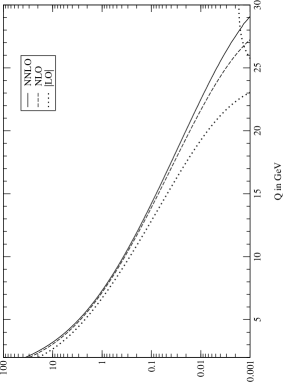
Figure 3: The cros section $d\Delta\sigma/dQ$ in pb/GeV plotted in the range $2<Q<30$ GeV at $\mu=Q$ in LO, NLO and NNLO.

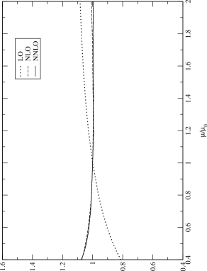
Figure 4: The polarized quantity $N(\mu/\mu_{0})$ plotted in the range $0.4<\mu/\mu_{0}<2$ with $Q=5$ GeV and $\mu_{0}=Q$.

2 Computational details

A different picture is shown by the invariant mass squared distribution given by

$$\frac{d\,\Delta\sigma}{dQ^{2}}=\frac{4\,\pi\,\alpha^{2}}{3\,N_{C}\,Q^{2}\,S}\,\Delta W\left(\tau,\frac{Q^{2}}{\mu^{2}}\right)\,,\quad\tau=\frac{Q^{2}}{S}\,.$$ (4)

The structure function $\Delta W$ equals

$$\Delta W\left(\tau,\frac{Q^{2}}{\mu^{2}}\right)=\sum_{a_{1},a_{2}=q,g}\int_{\tau}^{1}dx_{1}\,\int_{\tau/x_{1}}^{1}dx_{2}\,$$

$$\times\Delta f_{a_{1}}(x_{1},\mu^{2})\,\Delta f_{a_{2}}(x_{2},\mu^{2})\,$$

$$\times\Delta_{a_{1}a_{2}}\left(\tau,\frac{Q^{2}}{\mu^{2}}\right)\,.$$ (5)

Here the zeroth order quark-anti-quark process dominates so that this process is an excellent tool to measure the sea-quark density in proton-proton reactions. The NLO corrections to the coefficient function $\Delta_{a_{1}a_{2}}$ were calculated in [3] and the NNLO corrections have been recently computed in [4]. In higher order the quark-anti-quark process also dominates. If $\tilde{M}$ is the amplitude of a parton-parton subprocess then the $q\bar{q}$ is given by

$$q(p_{1},s_{1})+\bar{q}(p_{2},s_{2})\rightarrow\gamma^{*}+^{\prime}X^{\prime}\,,$$

$$|\Delta M_{q\bar{q}}|^{2} = \frac{1}{4}\,{\bf Tr}\,\left(\gamma_{5}{/\!\!\!}s_{2}\,({/\!\!\!}p_{2}-m)\,\tilde{M}\,\gamma_{5}{/\!\!\!}s_{1}\right.$$ (6)

$$\left.\times({/\!\!\!}p_{1}+m)\tilde{M}^{\dagger}\right)\,,$$

$$q_{1}(\bar{q}_{1})(p_{1},s_{1})+g(p_{2})\rightarrow\gamma^{*}+^{\prime}X^{\prime}\,,$$

$$|\Delta M_{qg}|^{2} = \frac{1}{4}\,\epsilon_{\mu\nu\lambda\sigma}\,\frac{p_{2}^{\lambda}\,l_{2}^{\sigma}}{p_{2}\cdot l_{2}}\,{\bf Tr}\,\left(\tilde{M}^{\mu}\,\gamma_{5}{/\!\!\!}s_{1}\right.$$ (7)

$$\left.\times({/\!\!\!}p_{1}\pm m)\,\tilde{M}^{\nu\dagger}\right)\,,$$

$$q_{1}(\bar{q}_{1})(p_{1},s_{1})+q_{2}(\bar{q}_{2})(p_{2},s_{2})\rightarrow\gamma^{*}+^{\prime}X^{\prime}$$

$$|\Delta M_{q_{1}q_{2}}|^{2} = \frac{1}{4}\,{\bf Tr}\,\left(\gamma_{5}{/\!\!\!}s_{2}\,({/\!\!\!}p_{2}\pm m)\,\tilde{M}\,\gamma_{5}{/\!\!\!}s_{1}\right.$$ (8)

$$\left.\times({/\!\!\!}p_{1}\pm m)\,\tilde{M}^{\dagger}\right)\,,$$

$$g(p_{1})+g(p_{2})\rightarrow\gamma^{*}+^{\prime}X^{\prime}\,,$$

$$|\Delta M_{gg}|^{2} = \frac{1}{4}\,\epsilon_{\mu_{2}\nu_{2}\lambda_{2}\sigma_{2}}\,\frac{p_{2}^{\lambda_{2}}\,l_{2}^{\sigma_{2}}}{p_{2}\cdot l_{2}}\,\epsilon_{\mu_{1}\nu_{1}\lambda_{1}\sigma_{1}}$$ (9)

$$\times\frac{p_{1}^{\lambda_{1}}\,l_{1}^{\sigma_{1}}}{p_{1}\cdot l_{1}}\,{\bf Tr}\,\left(\tilde{M}^{\mu_{1}\mu_{2}}\,\tilde{M}^{\nu_{1}\nu_{2}\dagger}\right)\,,$$

with the constraints

$$s_{i}\cdot p_{i}=0\,,\quad s_{i}\cdot s_{i}=-1\,,\quad l_{i}\cdot l_{i}=0\,.$$ (10)

All these reactions contain the $\gamma_{5}$-matrix and/or the Levi-Civita tensor. If we use $n$-dimensional regularization we have to find a prescription for these typical four dimensional objects. Here we choose the prescription of HVBM [5] or equivalently the one given by [6]. Choosing the latter we obtain the prescription

• Replace the $\gamma_{5}$-matrix by

  $$\gamma_{\mu}\,\gamma_{5} = \frac{i}{6}\,\epsilon_{\mu\rho\sigma\tau}\,\gamma^{\rho}\,\gamma^{\sigma}\,\gamma^{\tau}\quad\mbox{or}$$

  $$\gamma_{5} = \frac{i}{24}\,\epsilon_{\rho\sigma\tau\kappa}\,\gamma^{\rho}\,\gamma^{\sigma}\,\gamma^{\tau}\,\gamma^{\kappa}\,.$$

• Compute all matrix elements in $n$ dimensions.

• Evaluate all Feynman integrals and phase space integrals in $n$-dimensions.

• Contract the Levi-Civita tensors in four dimensions after the Feynman integrals and phase space integrals are carried out.

This procedure requires an intensive tensorial reduction of the loop-integrals as well as the phase space integrals. However the HVBM methods entails the presence of evanescent counter terms. They were calculated up to two-loop order in [7]. The result has the following structure

$$Z_{qq}^{5,{\rm NS},+} = \delta(1-x)+a_{s}\,S_{\varepsilon}\,\left(\frac{Q^{2}}{\mu^{2}}\right)^{\varepsilon/2}\,\Bigg{[}z^{(1)}_{qq}$$ (11)

$$+\varepsilon\bar{z}^{(1)}_{qq}\Bigg{]}+\hat{a}_{s}^{2}\,S_{\varepsilon}^{2}\,\left(\frac{Q^{2}}{\mu^{2}}\right)^{\varepsilon}$$

$$\times\Bigg{[}+\frac{1}{\varepsilon}\,\beta_{0}\,z^{(1)}_{qq}+z^{(2),{\rm NS},+}_{qq}\Bigg{]}\,,$$

where $a_{s}=\alpha_{s}(\mu^{2})/4\pi$ is the renormalized coupling constant. Further $\bar{z}^{(1)}_{qq}$ and $(Q^{2}/\mu^{2})^{k\varepsilon}$ are process dependent. The other constants are process independent. The latter also holds for the following pieces

$$Z_{qq}^{5,{\rm NS},-}=-\hat{a}_{s}^{2}\,S_{\varepsilon}^{2}\,\left(\frac{Q^{2}}{\mu^{2}}\right)^{\varepsilon}\,\Bigg{[}z^{(2),{\rm NS},-}_{qq}\Bigg{]}\,,$$ (12)

$$Z_{qq}^{5,{\rm PS}}=\hat{a}_{s}^{2}\,S_{\varepsilon}^{2}\,\left(\frac{Q^{2}}{\mu^{2}}\right)^{\varepsilon}\,\Bigg{[}z^{(2),{\rm PS}}_{qq}\Bigg{]}\,,$$ (13)

The constant $Z_{qq}^{5,{\rm NS},+}$ is chosen in such a way that the following relation holds

$$\left(Z_{qq}^{5,{\rm NS},+}\right)^{2}=-\frac{\Delta\hat{W}_{q\bar{q}}^{\rm NS}(\hat{a}_{s},Q^{2}/\mu^{2})}{\hat{W}_{q\bar{q}}^{\rm NS}(\hat{a}_{s},Q^{2}/\mu^{2})}$$ (14)

where $\hat{W}_{q\bar{q}}^{\rm NS}$ is the partonic structure function of the unpolarized reaction. We have to remove the spurious terms coming from the $\gamma_{5}$ and Levi-Civita prescription in the partonic structure function by using these evanescent counter terms. Since they are present in the (anti-)quark sector we have to form the following products

$$\left(Z_{qq}^{5}\right)^{-2}\,\Delta W_{q\bar{q}}\,,\quad\left(Z_{qq}^{5}\right)^{-1}\,\Delta W_{qg}\,,\quad$$

$$\left(Z_{qq}^{5}\right)^{-2}\,\Delta W_{qq}\,,\quad\Delta W_{gg}$$ (15)

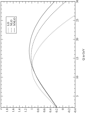
Figure 5: The longitudinal asymmetry $A_{LL}$ plotted in percent in the range $2<Q<30$ GeV at $\mu=Q$ in LO, NLO and NNLO.

3 Results

The processes which have to be calculated up to NNLO are

$$q+\bar{q}\rightarrow\gamma^{*}\,.$$ (16)

$$q+\bar{q}\rightarrow\gamma^{*}+g\,,$$ (17)

$$g+q(\bar{q})\rightarrow\gamma^{*}+q(\bar{q})\,.$$ (18)

$$q+\bar{q}\rightarrow\gamma^{*}+g+g\,,$$ (19)

$$g+q(\bar{q})\rightarrow\gamma^{*}+q(\bar{q})+g\,,$$ (20)

$$q+\bar{q}\rightarrow\gamma^{*}+q+\bar{q}\,,$$ (21)

$$q(\bar{q})+q(\bar{q})\rightarrow\gamma^{*}+q(\bar{q})+q(\bar{q})\,,$$ (22)

$$g+g\rightarrow\gamma^{*}+q+\bar{q}\,.$$ (23)

including virtual corrections to lower order processes. Apart from evanescent counter terms which are characteristic of the $\gamma_{5}$ and Levi-Civita prescription the calculation proceeds in the same way as in the unpolarized case. The renormalization and mass factorization are carried out in the ${\overline{MS}}$-scheme. We use the BB1 [8] parton density set to make our plots. The figures are constructed as follows

$LO$	$\Delta f^{LO}(x,\mu^{2})$	$\alpha_{s}^{LO}$
$NLO$	$\Delta f^{NLO}(x,\mu^{2})$	$\alpha_{s}^{NLO}$
$NNLO$	$\Delta f^{NLO}(x,\mu^{2})$	$\alpha_{s}^{NLO}$

Because of the lack of the three-loop anomalous dimensions we have no $\Delta f^{NNLO}$. Therefore in NNLO we use the NLO parton density set and the two-loop corrected running coupling constant $\alpha_{s}^{NLO}$. Further we set the mass factorization scale equal to the renormalization scale unless stated otherwise. Since we also compare with the unpolarized Drell-Yan process we choose the following parton density sets given by [9]. Since they have an approximate NNLO set we plot the figures according to

$LO$	$f^{LO}(x,\mu^{2})$	$\alpha_{s}^{LO}$
$NLO$	$f^{NLO}(x,\mu^{2})$	$\alpha_{s}^{NLO}$
$NNLO$	$f^{NNLO}(x,\mu^{2})$	$\alpha_{s}^{NNLO}$

Our findings are that the quark-anti-quark channel dominates the proton-proton reaction in polarized as well as well in unpolarized physics. The invariant mass distribution is shown in Fig. 3 in LO, NLO and NNLO. The K-factors defined by

$$K^{(i)}=\frac{\sigma^{(i)}}{\sigma^{LO}}\,,\qquad\Delta K^{(i)}=\frac{\Delta\,\sigma^{(i)}}{\Delta\,\sigma^{LO}}\,,$$ (24)

are roughly the same. For $Q=7~{}{\rm GeV}$ at $\sqrt{S}=200~{}{\rm GeV}$ we get a minimum. Here the values are $\Delta K^{NLO}=1.2$ and $\Delta K^{NNLO}=1.3$ respectively. In Fig. 4 we have plotted for $Q=5~{}{\rm GeV}$ the mass factorization scale dependence

$$N\left(\frac{\mu}{\mu_{0}}\right)=\frac{\Delta\sigma(\mu)}{\Delta\sigma(\mu_{0})}\,,$$ (25)

for $\mu_{0}=Q$ and $0.4\,\mu_{0}<\mu<2\,\mu_{0}$. We see a clear improvement while going from LO to NLO and surprisingly also from NLO to NNLO. In Fig. 5 we have shown the longitudinal asymmetry

$$A_{LL}=\frac{\Delta\,\sigma}{\sigma}\,,$$ (26)

in LO, NLO and NNLO. To compare the different polarized parton densities we have also plotted in Fig.6 the longitudinal asymmetry for the BB2 [8] and the GRSV standard (SS) and valence (VS) parametrizations [10]. The figure reveals that the largest gluon (BB1) leads to smallest asymmetry. On the other hand the smallest gluon (VS) gives the largest asymmetry. Notice that the latter parametrization produces the smallest asymmetry in the differential $p_{T}$-distribution.

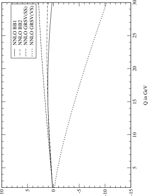
Figure 6: The longitudinal asymmetry $A_{LL}$ plotted in percent in the range $2<Q<30$ GeV at $\mu=Q$ and NNLO.

References

- [1] V. Ravindran, J. Smith, W.L. van Neerven, Nucl. Phys. B647 (2002) 275.
- [2] S. Chang, C. Coriano, R.D. Field, L.E. Gordon, Nucl. Phys. B512 (1998) 393.
- [3] P.G. Ratcliffe, Nucl. Phys. B223 (1983) 45.
- [4] V. Ravindran, J. Smith, W.L. van Neerven, Nucl. Phys. B682 (2004) 421.
-
[5]
G. ’t Hooft and M. Veltman, Nucl. Phys. B44 (1972) 189;
P. Breitenlohner and B. Maison, Commun. Math. 53 (1977) 11, 39, 55. - [6] D. Akyeampong and R. Delbourgo, Nuov. Cim. 17A (1973) 578, 18A (1973) 94, 19A (1974) 219.
- [7] Y. Matiounine, J. Smith, W.L. van Neerven, Phys. Rev. D58 (1998) 076002.
- [8] J. Blumlein, H. Böttcher, Nucl. Phys. B636 (2002) 225.
- [9] A.D. Martin, R.G. Roberts, W.J. Stirling, R.S. Thorne, Phys. Lett. B531 (2002) 216; Eur. Phys. J. C23 (2002) 73.
- [10] M. Glück, E. Reya, M. Stratmann, W. Vogelsang, Phys. Rev. D63 (2001) 094005.