Next-to-leading Log Resummation of Scalar and Pseudoscalar Higgs
Boson Differential Cross-Sections at the LHC and Tevatron

Abstract

The region of small transverse momentum in $q\bar{q}-$ and $gg-$initiated processes must be studied in the framework of resummation to account for the large, logarithmically-enhanced contributions to physical observables. In this paper, we will calculate the fixed order next-to-leading order (NLO) perturbative total and differential cross-sections for both a Standard Model (SM) scalar Higgs boson and the Minimal Supersymmetric Standard Model’s (MSSM) pseudoscalar Higgs boson in the Heavy Quark Effective Theory (HQET) where the mass of the top quark is taken to be infinite. Resummation coefficients $B^{(2)}_{g},C^{(2)}_{gg}$ for the total cross-section resummation for the pseudoscalar case are given, as well as $\bar{C}^{(1)}_{gg}$ for the differential cross-section.

I Introduction

The discovery of one or more Higgs bosons is the central research interest for high energy physics programs at hadron colliders around the world. Beyond the phenomenology of the Standard Model (SM) Higgs boson, the Minimal Supersymmetric Standard Model (MSSM) which is a special case of the Two Higgs Doublet Model (2HDM) is of particular interest to theorists. For a review see Ref. Gunion:1989we ; Carena:2002es .

Very recently, a new central value for the top quark mass was reportedGroup:2004rc . This changed the exclusion limits on the SM Higgs boson, putting its central mass value from precision electroweak fits at $117$ GeV/c². This is exciting because this value is above the exclusion limits from the LEP direct searches which exclude the mass of a SM-like Higgs boson below approximately $114$ GeV/c²Barate:2003sz . In the MSSM there are five physical Higgs bosons; a light and a heavy scalar ($h^{0}$,$H^{0}$), two charged scalars ($H^{\pm}$), and a CP-odd pseudoscalar ($A^{0}$). The mass of the pseudoscalar is excludedFernandez:2003hu from being lighter than $92$ GeV/c². The ratio between the vacuum expectation values (vevs) of the two neutral Higgs bosons of the MSSM is defined as $\tan\beta=v_{2}/v_{1}$. For $m_{\textrm{top}}=174.3$ GeV/c², $0.5<\tan\beta<2.4$ has been excluded by the LEP Higgs searches. The bounds on $\tan\beta$ will change as the central value of the top mass changes. A full analysis of the $\tan\beta$ exclusion bounds for the new top mass of $m_{\textrm{top}}=178.0$ GeV/c² is not yet available. In this paper, we will leave $\tan\beta=1$ so that the pseudoscalar results can easily be scaled by an appropriate number of interest to the reader, and the mass of the Higgs bosons will be set to $M_{\Phi}=120$ GeV/c², where $\Phi$ is the Higgs boson of interest.

In the context of resummation, the literature has focused on the scalar Higgs bosonCatani:ne ; Kauffman:1991jt ; Yuan:1991we ; Kauffman:cx ; Kramer:1996iq ; Catani:1996yz ; Balazs:2000wv ; deFlorian:2000pr ; deFlorian:2001zd ; Glosser:2002gm ; Berger:2002ut ; Berger:2003pd ; Bozzi:2003jy ; Catani:2003zt ; Kulesza:2003wn . This paper will provide resummation coefficients for the pseudoscalar Higgs boson for the total cross-section and differential distributions. Our calculations are done in the Heavy Quark Effective Theory (HQET) where the mass of the top quark is taken to be infinite. The role of the bottom quark in pseudoscalar production becomes dominant at large $\tan\beta$. In order to correctly take the bottom quark into account at this order, massive resummation coefficients will have to be determined. This will be reserved for another discussion.

In Section II, we will introduce the Heavy Quark Effective Theory (HQET) in which our calculations were performed. In Section III, we will introduce our resummation conventions and present our new results for pseudoscalar resummation. Finally, in Section IV we will present our numeric results for the differential distributions for the SM scalar and MSSM pseudoscalar Higgs boson at the Large Hadron Collider (LHC) and Tevatron in the HQET.

II Heavy Quark Effective Theory

Higgs phenomenology in QCD lends itself well to the use of Heavy Quark Effective Theory (HQET). When only the top quark is considered in calculations, it is possible to replace the top quark loops by an effective vertex when the other quarks are ignored. The role of the bottom quark in Higgs physics has recently been examined in great detailHarlander:2003ai ; Field:2003yy , but will not be included in this paper. The Lagrangian that describes this effective vertex can be derived from the $gg\rightarrow\Phi$ (where $\Phi$ is a Higgs boson of interest) triangle diagramWilczek:1977zn ; Ellis:1979jy ; Georgi:1977gs ; Rizzo:1979mf and letting the mass of the quark become infinitely heavy at the end of the calculationShifman:eb ; Vainshtein:ea ; Voloshin:hp . The Higgs of interest could be the SM scalar Higgs, or the pseudoscalar Higgs of the MSSM. In principle, the light and heavy scalar Higgs of the MSSM can be included in this formalism in place of the SM Higgs by multiplying by the appropriate coupling factor. However, supersymmetric corrections within the MSSM will not be included in this paper, only SM QCD corrections will be included.

The HQET method allows for the inclusion of the $\mathcal{O}(\epsilon)$ terms which are important for deriving resummation coefficients. This program leads to the effective Lagrangian in $d=4-2\epsilon$ dimensions for a scalar Higgs boson

$$\mathcal{L}_{\textrm{eff}}^{H}=-\frac{1}{4}g_{H}HG^{a}_{\mu\nu}G^{a,\mu\nu}\biggl{(}\frac{4\pi\mu_{r}^{2}}{m_{\textrm{top}}^{2}}\biggr{)}^{\epsilon}\Gamma(1+\epsilon)$$ (1)

where $g_{H}=\alpha_{\textrm{s}}/3\pi v$ is the coupling of the effective vertex at LO, $G^{a,\mu\nu}$ is the field-strength tensor for the gluons, $\mu_{r}$ is the renormalization scale, and the vacuum expectation value (vev) of the Higgs is defined as $v^{2}=(\sqrt{2}G_{F})^{-1}\simeq 246$ GeV. The effective coupling receives order by order corrections that have been calculatedChetyrkin:1997sg ; Kramer:1996iq previously. The appearance of the top quark mass in this expression hints that the corrections to the effective coupling at higher order may include logarithmic corrections including the top quark mass, which is the case. Alternatively, we can define $1/v^{2}=6422.91$ pb, which is convenient in cross-section calculations. This effective Lagrangian generates effective vertices with two, three, and four gluons with a scalar Higgs boson. The Feynman rules for a scalar Higgs can be found in the literatureKauffman:1996ix .

When a pseudoscalar Higgs boson is considered, the effective LO Lagrangian changes due to the $\gamma_{5}$ coupling and can be written

$$\mathcal{L}_{\textrm{eff}}^{A^{0}}=\frac{1}{4}g_{A^{0}}A^{0}G^{a}_{\mu\nu}\tilde{G}^{a,\mu\nu}\biggl{(}\frac{4\pi\mu_{r}^{2}}{m_{\textrm{top}}^{2}}\biggr{)}^{\epsilon}\Gamma(1+\epsilon)$$ (2)

where $g_{A^{0}}=\alpha_{\textrm{s}}/2\pi v$ is the coupling of the effective vertex. The $\tilde{G}^{a,\mu\nu}=1/2\,\epsilon^{\mu\nu\rho\sigma}G_{\rho\sigma}^{a}$ operator is the dual of the usual gluon field-strength tensor. It is important to note that the four gluon plus pseudoscalar Higgs vertex is absent in this effective Lagrangian as its Feynman rule is proportional to a completely antisymmetric combination of structure functions and therefore vanishes. It should be noted that this is the LO effective Lagrangian, and that a second operator begins to contribute at higher orders. A complete discussion can be found in Ref. Chetyrkin:1998mw . The Feynman rules for the pseudoscalar can be found in the literatureKauffman:1993nv . The Feynman rules listed in this reference should be used with $g_{A^{0}}=\alpha_{\textrm{s}}/2\pi v$ to avoid a spurious extra factor of $1/4$.

If we define $z=M_{\Phi}^{2}/\hat{s}$ where $\hat{s}$ is the partonic center of momentum energy squared, the partonic total cross-section for Higgs production (either scalar or pseudoscalar written here generically as $\Phi$) from the fusion of two partons $a$ and $b$ can be written as a series expansion in $\alpha_{\textrm{s}}$ as

$$\hat{\sigma}(ab\rightarrow\Phi+X) =\hat{\sigma}_{0}^{\Phi}\Delta_{ab\rightarrow\Phi}$$

$$=\hat{\sigma}_{0}^{\Phi}\biggl{(}\delta_{ag}\delta_{bg}\delta(1-z)+\frac{\alpha_{\textrm{s}}}{\pi}\Delta^{(1)}_{ab\rightarrow\Phi}(z)+\biggl{(}\frac{\alpha_{\textrm{s}}}{\pi}\biggr{)}^{2}\Delta^{(2)}_{ab\rightarrow\Phi}(z)+\mathcal{O}(\alpha_{\textrm{s}}^{3})+\cdots\biggr{)},$$ (3)

where $\hat{\sigma}_{0}^{\Phi}$ is the LO partonic total cross-section, and the $\Delta^{(n)}_{ab\rightarrow\Phi}(z)$ coefficients are higher order corrections.

The NNLO corrections for both the scalar and pseudoscalar Higgs bosons have been calculated in the HQETHarlander:2001is ; Harlander:2002vv ; Ravindran:2003um . Although the next-to-leading order corrections have been calculated in several placesDawson:1990zj ; Djouadi:1991tk ; Kauffman:1991jt ; Kauffman:cx ; Kauffman:1993nv ; Spira:1995rr ; Ravindran:2002dc ; Field:2002pb , there are some discrepancies in the literature that we would like to clear up in this paper. For this reason, we will explicitly calculate the NLO corrections for the $gg$ initial state. The importance of this particular channel, beyond its relevance to high-energy hadron collisions, will be addressed later. The partonic cross-section at NLO has to be written as the sum of the real emissions, the virtual corrections, the charge renormalization, and Altarelli-Parisi subtractions as follows

$$\hat{\sigma}_{\text{NLO}}=\hat{\sigma}_{\text{real}}+\hat{\sigma}_{\text{virt}}+\hat{\sigma}_{\text{ren}}+\hat{\sigma}_{\text{AP}}.$$ (4)

Although a few very thorough treatments for the scalar case exist in the literatureDawson:1990zj ; Djouadi:1991tk , we will re-derive them here to highlight differences in the pseudoscalar case, where an exhaustive treatment is missing. We will follow closely the discussion in these references. We will see that only the $gg$ channel will play a role in the resummation formalism.

II.1 Scalar Higgs Matrix Elements

Suppressing $\mathcal{O}(\epsilon)$ terms for now, the matrix elements for scalar Higgs production in the HQET can be written asDawson:1990zj ; Djouadi:1991tk ; Kauffman:1991jt ; Kauffman:cx ; Kauffman:1993nv ; Spira:1995rr ; Ravindran:2002dc ; Field:2002pb

$$\mathcal{M}(g(p_{1}^{\mu,A})+g(p_{2}^{\nu,B})\rightarrow H)=-\frac{\alpha_{\textrm{s}}}{3\pi v}\delta^{AB}\biggl{(}\eta^{\mu\nu}\frac{M_{H}^{2}}{2}-p_{1}^{\nu}p_{2}^{\mu}\biggr{)}\epsilon_{\mu}(p_{1})\epsilon_{\nu}(p_{2}).$$ (5)

Here $AB(\mu\nu)$ are the color (Lorentz) indices of the incoming gluons. When the matrix elements are squared, the contraction of the delta functions yields a factor of $\delta^{AB}\delta_{AB}=N_{c}^{2}-1=8$, the contraction of the metric yields $\eta^{\mu\nu}\eta_{\mu\nu}=d$. This yields the squared matrix elements (before any color-spin averaging)

$$|\mathcal{M}(gg\rightarrow H)|^{2}=\frac{\alpha_{\textrm{s}}^{2}M_{H}^{4}(N_{c}^{2}-1)}{16\pi^{2}v^{2}}\biggl{(}\frac{4\pi\mu_{r}^{2}}{m_{\textrm{top}}^{2}}\biggr{)}^{2\epsilon}\Gamma^{2}(1+\epsilon)(1-\epsilon).$$ (6)

In this $2\rightarrow 1$ process, it is easiest to calculate the decay width of the Higgs and convert that to a partonic total cross-section. We need to color and spin average the matrix elements squared noting that the gluon-gluon initial state must be averaged over $4(1-\epsilon)^{2}$ transverse polarizations. We can write the partonic cross-section in terms of the decay width and simply add $\delta(1-z)$ since $z=M_{H}^{2}/\hat{s}=1$ at threshold, so thatDawson:1990zj

$$\hat{\sigma}_{0}^{H}(gg\rightarrow H) =\frac{\pi^{2}}{8M_{H}^{3}}\,\Gamma(H\rightarrow gg)\,$$ (7)

$$=\biggl{(}\frac{\alpha_{\textrm{s}}}{\pi}\biggr{)}^{2}\frac{\pi}{576v^{2}}\biggl{(}\frac{4\pi\mu_{r}^{2}}{m_{\textrm{top}}^{2}}\biggr{)}^{2\epsilon}\frac{\Gamma^{2}(1+\epsilon)}{1-\epsilon}.$$

This factor (with its $\epsilon$ dependence) will be pulled from each of the higher order correction factors. The LO cross-section in the HQET starts at $\mathcal{O}(\alpha_{\textrm{s}}^{2})$.

II.1.1 Radiative Corrections

At the next order in perturbation theory, there are $qg$ and $q\bar{q}$ initial state processes. However, as we will see later, we are only interested in the $gg$ initial state, so we will only calculate the NLO corrections to the $gg$ initial state process.

The real contributions at NLO to the $gg$ initial state come from the process $gg\rightarrow gH$ which was originally calculated in the $\epsilon\rightarrow 0$ limit in the full theory including a finite mass top quark in Ref. Ellis:1987xu ; Baur:1989cm . We can write the amplitude as,

$$g(p_{1}^{A,\mu})+g(p_{2}^{B,\nu})\rightarrow g(-p_{3}^{C,\sigma})+H(-p_{5})$$ (8)

If we define the partonic (with hats) kinematic variables in terms of the Higgs momentum so that our differential cross-section can be written in terms of the Higgs transverse momentum as $\hat{s}=(p_{1}+p_{2})^{2}$, $\hat{t}=(p_{1}+p_{5})^{2}$, and $\hat{u}=(p_{2}+p_{5})^{2}$. The matrix elements take the symmetric formDawson:1990zj ; Djouadi:1991tk ; Kauffman:1991jt ; Kauffman:cx ; Kauffman:1993nv ; Spira:1995rr ; Ravindran:2002dc ; Field:2002pb

$$|\mathcal{M}(gg\rightarrow gH)|^{2}= \frac{\alpha_{\textrm{s}}^{3}}{v^{2}}\frac{4N_{c}(N_{c}^{2}-1)}{9\pi}\biggl{(}\frac{4\pi\mu_{r}^{2}}{m_{\textrm{top}}^{2}}\biggr{)}^{2\epsilon}\Gamma^{2}(1+\epsilon)$$

$$\times \biggl{\{}\biggl{[}\frac{M_{H}^{8}+\hat{s}^{4}+\hat{t}^{4}+\hat{u}^{4}}{\hat{s}\hat{t}\hat{u}}\biggr{]}(1-2\epsilon)+\frac{\epsilon}{2}\biggl{[}\frac{(M_{H}^{4}+\hat{s}^{2}+\hat{t}^{2}+\hat{u}^{2})^{2}}{\hat{s}\hat{t}\hat{u}}\biggr{]}\biggr{\}}.$$ (9)

Color and spin averaging gives an additional factor of $1/256/(1-\epsilon)^{2}$. By pulling out the LO cross-section from the expression, we can write the properly averaged matrix elements (where the overbar corresponds to color and spin averaging)

$$|\overline{\mathcal{M}}(gg\rightarrow gH)|^{2}=\hat{\sigma}_{0}^{H}\frac{\alpha_{\textrm{s}}}{\pi}\frac{N_{c}(N_{c}^{2}-1)}{1-\epsilon}\biggl{\{}\biggl{[}\frac{M_{H}^{8}+\hat{s}^{4}+\hat{t}^{4}+\hat{u}^{4}}{\hat{s}\hat{t}\hat{u}}\biggr{]}(1-2\epsilon)+\frac{\epsilon}{2}\biggl{[}\frac{(M_{H}^{4}+\hat{s}^{2}+\hat{t}^{2}+\hat{u}^{2})^{2}}{\hat{s}\hat{t}\hat{u}}\biggr{]}\biggr{\}}.$$

First, let us find the differential cross-section. The LO differential cross-section involves $2\rightarrow 2$ kinematics and can be written with the $4-2\epsilon$ phase space dimensions asKauffman:cx

$$\frac{d\hat{\sigma}^{H}}{d\hat{t}}=\frac{1}{16\pi\hat{s}^{2}}\biggl{(}\frac{4\pi\mu_{r}^{2}}{M_{H}^{2}}\biggr{)}^{\epsilon}\frac{1}{\Gamma(1-\epsilon)}\biggl{(}\frac{\hat{s}M_{H}^{2}}{\hat{u}\hat{t}}\biggr{)}^{\epsilon}|\overline{\mathcal{M}}|^{2}.$$ (10)

As we will see in Sec. III, it is the small $p_{t}$ behavior of this expression that we will be interested in. If we insert the expression $\hat{u}\hat{t}=\hat{s}p_{t}^{2}$ and drop the terms proportional to $p_{t}$, we find an expression for the differential cross-section in the small $p_{t}$ limit. Once we have changed variables, we find the partonic differential cross-section in the small $p_{t}$ region (where we are suppressing the trivial rapidity dependence)

$$\frac{d\hat{\sigma}^{H}}{dp_{t}^{2}}=\hat{\sigma}_{0}^{H}\frac{\alpha_{\textrm{s}}}{\pi}\biggl{(}\frac{4\pi\mu_{r}^{2}}{M_{H}^{2}}\biggr{)}^{\epsilon}\frac{z}{(1-\epsilon)\Gamma(1-\epsilon)}\biggl{(}\frac{M_{H}^{2}}{p_{t}^{2}}\biggr{)}^{\epsilon}\biggl{[}{C_{A}}\frac{1}{p_{t}^{2}}\ln\biggl{(}\frac{M_{H}^{2}}{p_{t}^{2}}\biggr{)}-\beta_{0}\frac{1}{p_{t}^{2}}\biggr{]}.$$ (11)

We will see that this representation will make it particularly simple to extract the resummation coefficients $A^{(1)}_{g}$ and $B^{(1)}_{g}$ for the differential distribution. These coefficients will be the same for the total cross-section as well. Turning our attention back to the expression we had for the matrix elements squared, we would like to calculate the real corrections for the NLO total partonic cross-section. The matrix elements for the real emission needs to be integrated and can be written asDawson:1990zj

$$\hat{\sigma}=\frac{1}{2\hat{s}}\int\overline{|\mathcal{M}|}^{2}\,\textrm{dPS}_{2}.$$ (12)

For a $2\rightarrow 2$ process, this can be done by introducing the following parameterization for the angular integration. If we write the scattering angle $\theta$ as $\cos\theta=2\omega-1$, this maps the $\theta$ integration to an $\omega$ integration between $0$ and $1$. We can express the kinematic invariants as follows

$$\hat{t}=-\hat{s}(1-z)(1-\omega),\quad\hat{u}=-\hat{s}(1-z)\omega,$$ (13)

and do the phase space integrations using the following parameterization

$$\textrm{dPS}_{2}=\frac{1}{8\pi}\biggl{(}\frac{4\pi\mu_{r}^{2}}{\hat{s}}\biggr{)}^{\epsilon}\frac{(1-z)^{1-2\epsilon}}{\Gamma(1-\epsilon)}\int^{1}_{0}\omega^{-\epsilon}(1-\omega)^{-\epsilon}d\omega$$ (14)

which reduces the angular integration into repeated applications of Euler’s beta function integral, where additional integer powers of $\omega$ and $(1-\omega)$ are introduced from the kinematic variables $\hat{t}$ and $\hat{u}$,

$$\int^{1}_{0}d\omega\,\omega^{\alpha}(1-\omega)^{\beta}=\frac{\Gamma(1+\alpha)\Gamma(1+\beta)}{\Gamma(2+\alpha+\beta)}.$$ (15)

Turning our attention back to the real emissions, we find the color and spin averaged partonic total cross-section, after regulating the singularity at $z=1$ with a plus distribution, can be written as

$$\hat{\sigma}_{\textrm{real}}^{H}=\hat{\sigma}_{0}^{H}\biggl{(}\frac{\alpha_{\textrm{s}}}{\pi}\biggr{)} \biggl{(}\frac{4\pi\mu_{r}^{2}}{\hat{s}}\biggr{)}^{\epsilon}\Gamma(1+\epsilon)$$

$$\times{C_{A}}\biggl{\{}\biggl{[} \frac{1}{\epsilon^{2}}+\frac{1}{\epsilon}+1-2{\zeta_{2}}\biggr{]}\delta(1-z)-\frac{2z}{\epsilon}\biggl{[}z{\mathcal{D}_{0}(z)}+\frac{1-z}{z}+z(1-z)\biggr{]}-\frac{11}{6}(1-z)^{3}$$

$$+2\biggl{[}1+z^{4}+(1-z)^{4}\biggr{]}{\mathcal{D}_{1}(z)}-2\biggl{[}1-z+2z^{2}+z^{4}{\mathcal{D}_{0}(z)}\biggr{]}\biggr{\}}+\mathcal{O}(\epsilon),$$ (16)

where the plus prescription is defined as usual

$$\int_{0}^{1}dx\,f(x)[g(x)]_{+}=\int_{0}^{1}dx\,g(x)[f(x)-f(1)],$$ (17)

and we have introduced the common abbreviation

$$\mathcal{D}_{n}(z)\equiv\biggl{(}\frac{\ln^{n}(1-z)}{1-z}\biggr{)}_{\!+\!}.$$ (18)

II.1.2 Virtual Corrections

Next, we must calculate the virtual contributions. There are two diagrams with gluon loops (a gluon triangle and a four point incoming state as can be seen in Ref. Dawson:1990zj ), and can be calculated directly. We can write the integrated virtual contribution that contributes at $\alpha_{\textrm{s}}^{3}$ to the total partonic cross-section in the same fashion as the real emissionsDawson:1990zj ; Djouadi:1991tk ; Kauffman:1991jt ; Kauffman:cx ; Kauffman:1993nv ; Spira:1995rr ; Ravindran:2002dc ; Field:2002pb ,

$$\hat{\sigma}_{\textrm{virt}}=\hat{\sigma}_{0}\biggl{(}\frac{\alpha_{\textrm{s}}}{\pi}\biggr{)}\biggl{(}\frac{4\pi\mu_{r}^{2}}{M_{H}^{2}}\biggr{)}^{\epsilon}\Gamma(1+\epsilon){C_{A}}\biggl{\{}\biggl{[}-\frac{1}{\epsilon^{2}}-\frac{1}{\epsilon}+\frac{5}{6}+4{\zeta_{2}}\biggr{]}\delta(1-z)\biggr{\}}.$$ (19)

As expected, the $\epsilon^{2}$ singularities cancel between the real emission and virtual graphs. It will turn out that the differences between the fixed order results for the scalar and the pseudoscalar come from different virtual corrections. These virtual contributions will be needed to cancel some $\epsilon$ poles in the expression we will derive to determine the process dependent resummation coefficients, in particular $C^{(1)}_{gg}$ for the differential distribution.

II.1.3 Total cross-section

The remaining $1/\epsilon$ singularities must be removed to find the partonic total cross-section. The poles are cancelled in the charge (coupling) renormalization and the Altarelli-Parisi subtraction. Understanding the charge renormalization tells us why is was so important to have the $\mathcal{O}(\epsilon)$ terms of the lowest order cross-section. We can see that the counter-term can be writtenDawson:1990zj ; Djouadi:1991tk

$$\hat{\sigma}_{\textrm{ren}}=(4Z_{g})\hat{\sigma}_{0},\quad Z_{g}=-\frac{\alpha_{\textrm{s}}}{\epsilon}(4\pi)^{\epsilon-1}\Gamma(1+\epsilon)\beta_{0},\quad\beta_{0}=\frac{11}{6}{{C_{A}}}-\frac{2}{3}{{n_{\!f}}{T_{\!R}}},$$ (20)

where ${n_{\!f}}=5$ since the top quark has been integrated out. These equations hold with the $\overline{\textrm{MS}}$ renormalization conditions.

The Altarelli-Parisi subtraction factors out the soft and collinear singularities into the PDFs much like the factorization process separates the short and long distance physics in hadron-hadron scattering. This cancels the rest of the $1/\epsilon$ poles and gives us the final expression for the total cross-section

$$\hat{\sigma}_{\textrm{NLO}}(gg\rightarrow H+X)=\hat{\sigma}_{0}^{H}\biggl{\{}\delta(1-z)+\biggl{(}\frac{\alpha_{\textrm{s}}}{\pi}\biggr{)} \biggl{[}\biggl{(}\frac{11}{6}{C_{A}}+2{C_{A}}{\zeta_{2}}\biggr{)}\delta(1-z)-\frac{11}{6}{C_{A}}(1-z)^{3}$$

$$+2{C_{A}}\biggl{[}1+z^{4}+(1-z)^{4}\biggr{]}{\mathcal{D}_{1}(z)} +2{C_{A}}\biggr{(}z^{2}{\mathcal{D}_{0}(z)}+(1-z)+z^{2}(1-z)\biggr{)}\ln\frac{M^{2}_{H}}{z\mu^{2}}\biggr{]}\biggr{\}}+\mathcal{O}(\epsilon).$$ (21)

Our expressions for the resummation coefficients show the their full color dependence. It is sufficient to notice at this stage that the term proportional to the $\delta(1-z)$ in the correction can be evaluated as $11/2+\pi^{2}$ when we use

$${{C_{A}}}={N_{\!c}},\quad{{C_{F}}}=\frac{{N^{\,2}_{\!c}}-1}{2{N_{\!c}}},\quad{{T_{\!R}}}=\frac{1}{2}.$$ (22)

II.2 Pseudoscalar Higgs Matrix Elements

There are many reasons for our primary interest to be the pseudoscalar Higgs boson. In the MSSM, the exact roles the top and bottom quarks play in the differential cross-section is complicatedField:2003yy . However, in much of the parameter space in the MSSM, the cross-section for the pseudoscalar is larger than the lightest scalar Higgs boson in the MSSM. If supersymmetry does exist in nature, the pseudoscalar Higgs may be the first Higgs boson discovered due to its larger cross-section. If supersymmetry becomes important only at very high scales, then seeing a pseudoscalar Higgs would be the first evidence of supersymmetry in nature. This leads us to investigate in detail pseudoscalar resummation.

We should also mention that because of the importance of the bottom quark in calculations involving the MSSM pseudoscalar (and the lightest scalar Higgs in the MSSM as well) when the parameter $\tan\beta$ is large is systematically ignored in these calculations. To remedy this situation, one would have to calculate the resummation coefficients in the full theory. In principle, these coefficients can be extracted from Ref. Spira:1995rr . However, these results have not been published.

The difference in the lowest order (LO) partonic cross-section of the pseudoscalar Higgs boson and the scalar Higgs boson can be traced to the difference in the effective couplings $g_{H}$ and $g_{A^{0}}$ and a factor of $9/4$. This can be written asKauffman:1993nv

$$\hat{\sigma}_{0}^{A^{0}}(gg\rightarrow A^{0}) =\frac{9}{4}\hat{\sigma}_{0}^{H}(gg\rightarrow H)$$ (23)

$$=\biggl{(}\frac{\alpha_{\textrm{s}}}{\pi}\biggr{)}^{2}\frac{\pi}{256v^{2}}\biggl{(}\frac{4\pi\mu_{r}^{2}}{m_{\textrm{top}}^{2}}\biggr{)}^{2\epsilon}\frac{\Gamma^{2}(1+\epsilon)}{1-\epsilon}\,\delta(1-z).$$

Upon the expansion of the $\mathcal{O}(\epsilon)$ terms, we see they do not effect the final answer as expected at the lowest order.

II.2.1 Radiative Corrections

The matrix elements for the production of the pseudoscalar in the HQET are slightly more complicated in $d=4-2\epsilon$ dimensions due to the presence of the intrinsically $4$-dimensional Levi-Civita tensor in the Feynman rulesKauffman:1993nv coming from the $\tilde{G}^{a,\mu\nu}$ term in the effective Lagrangian. There are several conventions for handling this problem'tHooft:fi ; Akyeampong:xi ; Akyeampong:1973vk ; Akyeampong:1973vj . We have chosen the scheme defined in Ref. Akyeampong:xi ; Akyeampong:1973vk ; Akyeampong:1973vj .

For the radiative corrections, we can separate all the vectors into $4$- and $(d-4)$-dimensional components. We label the $(d-4)$-dimensional components of the vectors with a twiddle. We can take the incoming momentum to be $4$-dimensional as a convenient choice of frame, which simplifies the results considerablyKauffman:1993nv .

The (un-averaged) matrix elements can be written,

$$|\mathcal{M}(gg\rightarrow gA^{0})|^{2}= \frac{\alpha_{\textrm{s}}^{3}}{v^{2}}\frac{N_{c}(N_{c}^{2}-1)}{\pi}\biggl{(}\frac{4\pi\mu_{r}^{2}}{m_{\textrm{top}}^{2}}\biggr{)}^{2\epsilon}\Gamma^{2}(1+\epsilon)$$

$$\times \biggl{\{}\biggl{[}\frac{M_{A^{0}}^{8}+\hat{s}^{4}+\hat{t}^{4}+\hat{u}^{4}}{\hat{s}\hat{t}\hat{u}}\biggr{]}+\frac{2\hat{s}(\hat{t}^{2}+\hat{u}^{2})(\tilde{p}_{3}\!\cdot\!\tilde{p}_{3}\hat{s}-\hat{t}\hat{u}\epsilon)}{\hat{t}^{2}\hat{u}^{2}}\biggr{\}}.$$ (24)

We can see that the $\epsilon\rightarrow 0$ corrections are identical in the scalar and pseudoscalar case for the real emissions. We can also see that the residual difference is not only proportional to $\epsilon$, but rather proportional to $\epsilon$ and the $(d-4)$-dimensional component of the $p_{3}$ vector, which vanishes in the $4$-dimensional limit.

From this analysis, we can see that the real part of the differential cross-section for the pseudoscalar Higgs boson will be identical to the scalar case in Equation (11) with a $9/4$ difference in normalization.

II.2.2 Virtual Corrections

The virtual corrections to the pseudoscalar have the same diagrams as the scalar at this order, but there is a slight difference in the result. This difference is due to the fact that the diagram with the four point gluon vertex vanishes due to the antisymmetry of the $ggA^{0}$ vertex in the effective theory. The integrated result is

$$\hat{\sigma}_{\textrm{virt}}^{A^{0}}=\hat{\sigma}_{0}^{A^{0}}\biggl{(}\frac{\alpha_{\textrm{s}}}{\pi}\biggr{)}\biggl{(}\frac{4\pi\mu_{r}^{2}}{M_{H}^{2}}\biggr{)}^{\epsilon}\Gamma(1+\epsilon){C_{A}}\biggl{\{}\biggl{[}-\frac{1}{\epsilon^{2}}-\frac{1}{\epsilon}+2+4{\zeta_{2}}\biggr{]}\delta(1-z)\biggr{\}}.$$ (25)

We can see that although the pole terms are the same, the finite terms have changed slightly because of the “missing” diagram.

II.2.3 Total cross-section

When we combine our pseudoscalar results, we find that the total partonic cross-section that is identical to the scalar case with the exception of the small numeric difference in the $\delta(1-z)$ term. The expression changes from $11/6{C_{A}}+2{C_{A}}{\zeta_{2}}\rightarrow 2{C_{A}}+2{C_{A}}{\zeta_{2}}$ in the pseudoscalar case. Here we see the factor $11/2\rightarrow 6$, which would seem to be a small difference, but it is mostly a coincidence of the $\textrm{SU}_{3}$ Casimir invariants.

The partonic cross-section can be written as

$$\hat{\sigma}^{A^{0}}_{\textrm{NLO}}(gg\rightarrow A^{0}+X)=\hat{\sigma}_{0}^{A^{0}}\biggl{\{}\delta(1-z)+\biggl{(}\frac{\alpha_{\textrm{s}}}{\pi} \biggr{)}\biggl{[}\biggl{(}2{C_{A}}+2{C_{A}}{\zeta_{2}}\biggr{)}\delta(1-z)-\frac{11}{6}{C_{A}}(1-z)^{3}$$

$$+2{C_{A}}\biggl{[}1+z^{4}+(1-z)^{4}\biggr{]}\mathcal{D}_{1}(z) +2{C_{A}}\biggr{(}z^{2}{\mathcal{D}_{0}(z)}+(1-z)+z^{2}(1-z)\biggr{)}\ln\frac{M^{2}_{H}}{z\mu^{2}}\biggr{]}\biggr{\}}+\mathcal{O}(\epsilon).$$ (26)

Now that we have expressions for the total partonic cross-sections for both the scalar and the pseudoscalar Higgs boson we see that the only difference between the two lies in the correction proportional to $\delta(1-z)$ at NLO and in the normalization. This difference in the $\delta(1-z)$ factors is numerically small and is $\alpha_{\textrm{s}}$ suppressed, leaving us to believe that the primary difference is going to be factor of $9/4$ in the LO partonic cross-sections.

III Resummation

To introduce the machinery behind resummationCollins:1981uk ; Collins:va ; Collins:1984kg , we need to define the hadronic cross-section. This is the convolution of parton distributions functions (PDFs) with the partonic cross-section

$$\sigma(S,M_{\Phi}^{2})=\sum_{a,b}\int_{x_{1,\textrm{min}}}^{1}\!\!dx_{1}\int_{x_{2,\textrm{min}}}^{1}\!\!dx_{2}\,f_{a/h_{1}}(x_{1},\mu_{f})\,f_{b/h_{2}}(x_{2},\mu_{f})\,\int_{0}^{1}dz\,z\,\hat{\sigma}_{0}^{\Phi}\Delta_{ab\rightarrow\Phi}(z,\mu_{r},\mu_{f})$$ (27)

where $\mu_{r}$ and $\mu_{f}$ are the renormalization and factorization scales respectively, and $f_{a/h_{1}}\!$ is the parton distribution function for finding a parton $a$ in hadron $h_{1}$. We must also remember that there is a $\delta(1-z)$ in the definition of the LO cross-section $\hat{\sigma}_{0}^{\Phi}$. The minimum partonic energy fraction $x_{(1,2),\textrm{min}}$ is defined so that there is enough center of momentum energy to create the desired final state particles. A similar equation can be written for the differential distribution.

Implicitly, the partonic cross-section contains logarithmic corrections that are formally singular at threshold ($z\rightarrow 1$). The differential cross-section contains corrections that are singular as the transverse momentum of the Higgs particle vanishes. They can be written in the form

$$\textrm{threshold}\sim\alpha_{\textrm{s}}^{n}\frac{\ln^{2n-1}(1-z)}{(1-z)},\quad\textrm{recoil}\sim\frac{\alpha_{\textrm{s}}^{n}}{p_{t}^{2}}\ln^{2n-1}\frac{M_{\Phi}^{2}}{p_{t}^{2}},$$ (28)

and various powers of these combinations. It can be seen then that the normal fixed order cross-section calculation diverges (in one direction or the other) at small $p_{t}$ due to large logarithms, and therefore it is not reliable in this region. The systematic way of handling these formally divergent terms at small $p_{t}$ is known as resummation. Because of this divergent behavior, one is not usually able to integrate the differential cross-section all the way down to $p_{t}=0$ or to reliably understand the differential cross-section in the experimentally interesting small $p_{t}$ region. Resummation coefficients can be determined for both differential distributions and total-cross sections to address this problem.

III.1 Formalism

The resummation formalism allows the small $p_{t}$ cross-section to be written as a power series in both universal and process dependent coefficients. We write the resummed differential cross-section for a $c\bar{c}\rightarrow\Phi$ process (where $c$ in this case represents a gluon or a quark)

$$\frac{d\sigma^{\textrm{resum}}}{dp_{t}^{2}\,dy\,d\phi}=\sum_{a,b}\int_{x_{1,\textrm{min}}}^{1}\!\!\!dx_{1}\int_{x_{2,\textrm{min}}}^{1}\!\!\!dx_{2}\int_{0}^{\infty}db\,\frac{b}{2}J_{0}(bp_{t})\,f_{a/h_{1}}\!(x_{1},b_{0}/b)\,f_{b/h_{2}}\!(x_{2},b_{0}/b)\,\frac{S}{Q^{2}}W_{ab}(x_{1}x_{2}S;Q,b,\phi),$$ (29)

$$W_{ab}(s;Q,b,\phi)=\sum_{c}\int_{0}^{1}dz_{1}\int_{0}^{1}dz_{2}\,\bar{C}_{ca}(\alpha_{\textrm{s}}(b_{0}/b),z_{1})\,\bar{C}_{\bar{c}b}(\alpha_{\textrm{s}}(b_{0}/b),z_{2})\,\delta(Q^{2}-z_{1}z_{2}s)\,\frac{d\sigma_{\bar{c}c}^{LO}}{d\phi}\,S_{c}(Q,b),$$ (30)

where the Higgs mass $M_{\Phi}^{2}=Q^{2}$, $d\phi$ is the phase space of the system under consideration, and $\hat{\sigma}^{(LO)}_{c\bar{c}}$ is the lowest order cross-section with a $c\bar{c}$ initial state which is therefore defined at $p_{t}=0$. The constant $b_{0}$ is written in terms of the Euler-Mascheroni constant $\gamma_{E}=0.57721\ldots$ as $b_{0}=2e^{-\gamma_{E}}$. In the resummation formalism only the $gg$ and $q\bar{q}$ initial states are needed to determine the hadronic differential distribution at small $p_{t}$. The $qg$ initial states are accounted for in the cross terms in the convolution. The coefficients $C_{ab}$ are process dependent and can be written as power series to be described below. $J_{0}(bp_{t})$ is the first order Bessel function. The Sudakov form factor $S_{c}$, which makes the integration over the Bessel function convergent, can be written as

$$S_{c}(Q,b)=\exp\biggl{\{}-\int^{Q^{2}}_{b_{0}^{2}/b^{2}}\frac{dq^{2}}{q^{2}}\biggl{[}A_{c}(\alpha_{\textrm{s}}(q))\ln\frac{Q^{2}}{q^{2}}+B_{c}(\alpha_{\textrm{s}}(q))\biggr{]}\biggr{\}}.$$ (31)

The coefficient functions $A_{c}$, $B_{c}$, and $C_{ab}$ can be written as power series in $\alpha_{\textrm{s}}$ as

$$A_{c}(\alpha_{\textrm{s}})=\sum_{n=1}^{\infty}\biggl{(}\frac{\alpha_{\textrm{s}}}{\pi}\biggr{)}^{n}A_{c}^{(n)},\quad B_{c}(\alpha_{\textrm{s}})=\sum_{n=1}^{\infty}\biggl{(}\frac{\alpha_{\textrm{s}}}{\pi}\biggr{)}^{n}B_{c}^{(n)},$$ (32)

$$\bar{C}_{ab}(\alpha_{\textrm{s}},z)=\delta_{ab}\delta(1-z)+\sum_{n=1}^{\infty}\biggl{(}\frac{\alpha_{\textrm{s}}}{\pi}\biggr{)}^{n}\bar{C}_{ab}^{(n)}(z).$$ (33)

The $A^{(1)}_{c}$, $A^{(2)}_{c}$, and $B^{(1)}_{c}$ coefficients have been shown to be universal. There are several conventions in the literature as to whether to expand in terms of $\alpha_{\textrm{s}}/\pi$ or $\alpha_{\textrm{s}}/2\pi$ (or even $\alpha_{\textrm{s}}/4\pi$ in Ref. Ravindran:2003um ). We have chosen to expand in $\alpha_{\textrm{s}}/\pi$. It would seem that several typos exist in the literature due to this numeric expansion factor. We have derived the previously unknown coefficients $B^{(2)}_{g}$, $C^{(1)}_{gg}$ and $C^{(2)}_{gg}$ for pseudoscalar Higgs production for the total cross-section and the $\bar{C}^{(1)}_{gg}$ for the differential cross-section resummation given below. Here we must stop to address a question of notation. It is unfortunate that we have the same notation for the resummation coefficients for both the $p_{t}$ resummation and the total cross-section resummation. It would be convenient to use a calligraphic font for the $p_{t}$ coefficients, but several authors have used this font in other contexts dealing with resummation. Therefore, we will put bars over the resummation coefficients for differential cross-sections even if they are identical to the coefficients for the total cross-section resummation.

To determine the $\bar{C}^{(n)}$ coefficients for the differential cross-section, one must understand the meaning of the resummation formula. We can expand Equation (29) order by order in $\alpha_{\textrm{s}}$ and compare to the perturbative calculation to read off the coefficientsdeFlorian:2001zd . To extract the coefficients from the perturbative results, we need to integrate the differential cross-section around $p_{t}=0$ paying careful attention to the use of the Altarelli-Parisi splitting functions near $p_{t}=0$ as follows

$$\Delta\hat{\sigma}=\int_{0}^{q_{t}^{2}}dp_{t}^{2}\frac{d\hat{\sigma}}{dp_{t}^{2}}.$$ (34)

This expression will contain $\epsilon$ poles and virtual corrections at the next order will be needed to be added to find a finite expression. This is demonstrated later in this paper. One should also be careful to use this formula with other quantities that show the same rapidity dependence. When we expand to $\mathcal{O}(\alpha_{\textrm{s}})$, we can see that the NLL coefficients emerge as follows for a $c\bar{c}$ initial state

$$\Delta\hat{\sigma}_{c\bar{c}}=1+\frac{\alpha_{\textrm{s}}}{\pi}\biggl{[}-\frac{\bar{A}^{(1)}_{c}}{2}\ln^{2}\biggl{(}\frac{M_{\Phi}^{2}}{q_{t}^{2}}\biggr{)}-\bar{B}^{(1)}_{c}\ln\biggl{(}\frac{M_{\Phi}^{2}}{q_{t}^{2}}\biggr{)}+2\bar{C}^{(1)}_{c\bar{c}}\biggr{]}.$$ (35)

In principle, it is possible to continue this process to higher orders to obtain the needed coefficients for the differential cross-section. The NLO corrections to the differential cross-section are knownGlosser:2002gm ; Ravindran:2002dc , however the NNLO differential cross-section for Higgs production is currently unknown. However, the total cross-section is known to NNLO, so the resummation coefficients for the total cross-section can be determined to NNLL. The NLO differential cross-section in Ref. Glosser:2002gm has been written in terms of the $p_{t}$ of the Higgs boson for the scalar case, and could in principle be used in part to extract the NNLO process dependent $\bar{C}^{(2)}_{gg}$ coefficient for the differential cross-section for the scalar Higgs boson, advancing the resummed expressions ahead of the fixed order calculation. This work has not yet been completed.

III.2 Matching

The resummation formalism is valid in the small $p_{t}$ region. Fixed order perturbation theory is valid at moderate $p_{t}$ where there are no large logarithms. The process of matching allows for a smooth transition between the two regions. The procedure is described in great detail and clarity in Ref. Arnold:1990yk .

One can write the differential cross-section as the sum of three terms

$$\frac{d\sigma}{dp_{t}^{2}\,dy}=\frac{d\sigma^{\textrm{resum}}}{dp_{t}^{2}\,dy}+\frac{d\sigma^{\textrm{pert}}}{dp_{t}^{2}\,dy}-\frac{d\sigma^{\textrm{asym}}}{dp_{t}^{2}\,dy}$$ (36)

This equation is easy to understand. At low $p_{t}$, we have the resummed contribution since the latter contributions cancel. At high $p_{t}$ we have the perturbative contribution when the resummed and asymptotic cancel. At small $p_{t}$ we remove the terms from the perturbative expansion that are asymptotically divergent like $1/p_{t}^{2}$. This allows for a smooth transition between the two regions at all values of $p_{t}$. However, extracting the divergent pieces can be quite difficult analytically as one must express the differential cross-section in terms of $p_{t}$ order by order. For a $2\rightarrow 1$ process, the first order corrections have $2\rightarrow 2$ kinematics and this is relatively simple, but becomes more intractable for the higher order corrections.

In this paper, we are interested in the new coefficient functions, and determining where the distributions peak for the different colliders, so this treatment will be ignored. However, we will display the perturbative differential cross-section to guide the eye on what the transition must look like.

III.3 Higgs Resummation

One of the interesting facets for Higgs production is that there is only a $gg$ initial state for this process in the HQET at order $\alpha_{\textrm{s}}^{3}$, so the other terms (a $q\bar{q}$ initial state) are zero explicitly. Without getting too far ahead of our discussion, we can see that the Mellin moments of the $q\bar{q}$ corrections at order $\alpha_{\textrm{s}}^{4}$ strictly vanish on threshold due to the fact that there is no $q\bar{q}$ initial state at lowest order. This makes it possible to work in $z$-space with little additional effort due to the presence of the $\delta(1-z)$ terms in the $C^{(n)}_{gg}$ coefficients, which makes the convolution with the PDFs trivial.

An additional complication arises from evaluating the parton distribution functions at very low scales during the convolution. This is solved by what is known as the $b_{\star}$ prescriptionArnold:1990yk ; Davies:1984hs . Here the $b$ parameter is replaced by $b_{\star}$ that has an infrared cut-off $b_{\text{max}}$ so that as $b$ becomes large, $b_{\star}\rightarrow b_{\text{max}}$, and the fraction $b_{0}/b$ in Equation (29) never leaves the perturbative regime of the parton distribution function. Over the rest of the range $b_{\star}\approx b$. This can be achieved by in the following parametrization

$$b_{\star}=\frac{b}{\sqrt{1+b^{2}/b^{2}_{\textrm{max}}}}.$$ (37)

This construction may seem a little artificial, but it allows for the numeric integration of our differential cross-section and allows us to use what is known to make reasonable calculations.

In these calculations, we have set $b_{\text{max}}=(2$ GeV$)^{-1}$. This is mostly determined by the limits of applicability for the PDFs implemented to obtain the hadronic cross-section. There are other non-perturbative correction factors that are employedBerger:2002ut ; Berger:2003pd ; Arnold:1990yk , but as no data is available yet we have not included these factors in our analysis.

It is thus possible to determine the unknown coefficients to a given order in the resummation and preform the resummed calculation. The known coefficients for scalar Higgs production will be given later. To leading-log (LL) accuracy, only the $A^{(1)}_{c}$ term is needed. At next-to-leading log (NLL) accuracy one needs the $A^{(2)}_{c}$, $B^{(1)}_{c}$, and $C^{(1)}_{ab}$ coefficients. The state of the art currently is NNLL where the $A^{(3)}_{c}$, $B^{(2)}_{c}$, and $C^{(2)}_{ab}$ coefficients are neededdeFlorian:2001zd . For a scalar Higgs, these terms have been recently calculated but are missing for a pseudoscalar Higgs. The $A^{(3)}_{g}$ term can now be determined thanks to the excellent recent work on the three-loop splitting functionsVogt:2004mw ; Moch:2004pa . Previously, only a numeric estimate was availableVogt:2000ci .

Let us begin by extracting the process dependent $C_{ab}$ coefficients for the total cross-section. To extract the formally divergent pieces of the cross-section, consider the Mellin transform of the hadronic cross-section, $\sigma_{N}(M_{\Phi}^{2})$. The $N-$moments in Mellin space are defined as

$$\sigma_{N}(M_{\Phi}^{2})\equiv\int_{0}^{1}dz\,z^{N-1}\,\sigma(z,M_{\Phi}^{2})$$ (38)

The advantage of transforming to Mellin space is that the limit $z\rightarrow 1$ corresponds to the limit of $N\rightarrow\infty$. This allows for a systematic way of extracting the divergent terms, which diverge as $\ln(N)$ in Mellin space.

Before continuing, we should comment on which initial state channels contribute. In evaluating the the $C_{ab}$ coefficients in the $N\rightarrow\infty$ limit we see that only the $gg$ channel has finite contributions, all the other channels have Mellin moments are strictly zero on threshold. We could also see that in the HQET there are no $q\bar{q}$ or $qg$ initial state that contribute at this order to the cross-section at $p_{t}=0$. Although we have set up our formalism for the sum of several channels, we will now consider only the $gg$ initial state channel.

The Mellin moments of the fixed order corrections allow us to determine the process dependent total cross-section $C^{(n)}_{gg}$ coefficients in a simple way. We find the Mellin moments of the fixed order corrections, $\Delta^{(n)}_{ab\rightarrow\Phi}$, with the package harmpol in formVermaseren:2000nd . Some diverge as $\ln(N)$, most tend to zero as $N\rightarrow\infty$, and some finite pieces are left over. In this way, we can separate the formally divergent pieces from the finite contributions on threshold. With this we can identify the $p_{t}$ divergent terms with the $\ln(N)$ divergent terms in the Mellin moment. We choose to absorb the extra powers of $\gamma_{E}$ into our definition of $\tilde{N}=Ne^{\gamma_{E}}$ so that we do not have spurious factors of $\gamma_{E}$ in our expressions. This seems to be appropriate as in the $\overline{\textrm{MS}}$ scheme the factors of $\gamma_{E}$ are also absorbed. This being noted, we will continue to write our terms as $\ln(N)$ with no factors of $\gamma_{E}$.

III.3.1 Next-to-leading-log Differential Cross-section Coefficients

We are interested in determining the $C^{(1)}_{gg}$ coefficient for the scalar and pseudoscalar Higgs boson. First, let us integrate the differential cross-section for the scalar around $p_{t}=0$. We will label this contribution ‘real’ to note that this integral is similar to the real emission corrections to the total cross-section. We find

$$\Delta\hat{\sigma}^{\textrm{real}}=\hat{\sigma}_{0}^{H}\biggl{(}\frac{4\pi\mu_{r}^{2}}{M_{H}^{2}}\biggr{)}^{\epsilon}z\Gamma(1+\epsilon)(1+\epsilon)\frac{\alpha_{\textrm{s}}}{\pi}\biggl{[}\frac{{C_{A}}}{\epsilon^{2}}+\frac{\beta_{0}}{\epsilon}-\frac{{C_{A}}}{2}\ln^{2}\biggl{(}\frac{M_{H}^{2}}{q_{t}^{2}}\biggr{)}+\beta_{0}\ln\biggl{(}\frac{M_{H}^{2}}{q_{t}^{2}}\biggr{)}+{C_{A}}-{C_{A}}{\zeta_{2}}\biggr{]}.$$ (39)

We have to add the total partonic cross-section virtual correction to this expression to cancel the $\epsilon$ poles. The pole proportional to the $\beta_{0}$ gets renormalized into the coupling like in the total cross-section calculation. Once these two expression are added together we find

$$\Delta\hat{\sigma}=\hat{\sigma}_{0}^{H}z\biggl{[}1+\frac{\alpha_{\textrm{s}}}{\pi}\biggl{(}-\frac{{C_{A}}}{2}\ln^{2}\biggl{(}\frac{M_{H}^{2}}{q_{t}^{2}}\biggr{)}+\beta_{0}\ln\biggl{(}\frac{M_{H}^{2}}{q_{t}^{2}}\biggr{)}+{C_{A}}+\frac{5}{6}{C_{A}}+3{C_{A}}{\zeta_{2}}\biggl{)}\biggr{]}.$$ (40)

The coefficients can now be read off and agree with the literatureKauffman:cx

$$\bar{A}^{(1),H}_{g}={{C_{A}}},\quad\bar{B}^{(1),H}_{g}=-\beta_{0}=-\biggl{(}\frac{11}{6}{{C_{A}}}-\frac{2}{3}{{n_{\!f}}{T_{\!R}}}\biggr{)},\quad\bar{C}^{(1),H}_{gg}=\frac{11}{12}{{C_{A}}}+\frac{3}{2}{{C_{A}}}{\zeta_{2}}.$$ (41)

As noted earlier, the pseudoscalar Higgs has different virtual corrections from the scalar Higgs boson. This changes the $\bar{C}^{(1)}_{gg}$ coefficient for the pseudoscalar to

$$\bar{C}^{(1),A^{0}}_{gg}={{C_{A}}}+\frac{3}{2}{{C_{A}}}{\zeta_{2}}.$$ (42)

The pseudoscalar $\bar{C}^{(1)}_{gg}$ coefficient is larger that the scalar coefficient by a factor of $1/12{C_{A}}$. This is a small numeric difference, and the NNLL coefficient have not been extracted for the differential distribution, although as we will see in the next section we might expect a larger difference to appear in the differential $\bar{C}^{(2)}_{gg}$ coefficient based on the differences in the $C^{(2)}_{gg}$ coefficients for the total cross-section.

III.3.2 Next-to-leading-log Total Cross-section Coefficients

Exact expressions for the fixed order NLO corrections to scalar and pseudoscalar Higgs production have been in the literature for some time. Leaving aside the Sudakov terms ($A^{(n)}$ and $B^{(n)}$), let us examine our expressions for the fixed order corrections to the partonic cross-section. We see that the NLO corrections have organized themselves in terms of constant pieces proportional to $\delta(1-z)$ from the soft and virtual corrections and additional logarithmic corrections. The Mellin moment of the $\delta(1-z)$ is simply

$$\int_{0}^{1}dz\,z^{N-1}\,\delta(1-z)=1.$$ (43)

So it is easy to see that all the constant terms proportional to $\delta(1-z)$ contribute to the $C_{gg}^{(1)}$ term. Beyond these terms, the Mellin moments of the logarithmic corrections in the limit $N\rightarrow\infty$ can have finite pieces that also contribute. Once the expression for the correction term has been transformed into Mellin space, there are no terms proportional to $\delta(1-z)$, but are only constant terms.

In presenting the expressions for the $C_{gg}^{(n)}$ terms, we mix the notation somewhat to allow the reader to see all the different contributions. We keep the $\ln(N)$ pieces that are formally divergent, we separate out the terms that were initially proportional to the $\delta(1-z)$ for convenience, and we include the terms proportional to $\ln(M^{2}_{\Phi}/\mu^{2})$ for completeness. We have set $\mu=\mu_{r}=\mu_{f}$ for simplicity. The finite pieces compose the $C_{gg}^{(n)}$ coefficients.

In the case of the scalar and pseudoscalar

$$\Delta^{(1),H}_{N,gg}=\lim_{N\rightarrow\infty}\int_{0}^{1}dz\,z^{N-1}\Delta^{(1)}_{gg\rightarrow H}={{C_{A}}}\ln^{2}(N)-2{{C_{A}}}\ln\frac{M^{2}_{H}}{\mu^{2}}\ln(N)+\biggl{[}\frac{11}{6}{{C_{A}}}+2{{C_{A}}}{\zeta_{2}}\biggr{]}+2{{C_{A}}}{\zeta_{2}},$$ (44)

$$\Delta^{(1),A^{0}}_{N,gg}=\lim_{N\rightarrow\infty}\int_{0}^{1}dz\,z^{N-1}\Delta^{(1)}_{gg\rightarrow A^{0}}={{C_{A}}}\ln^{2}(N)-2{{C_{A}}}\ln\frac{M^{2}_{A^{0}}}{\mu^{2}}\ln(N)+\biggl{[}2{{C_{A}}}+2{{C_{A}}}{\zeta_{2}}\biggr{]}+2{{C_{A}}}{\zeta_{2}},$$ (45)

where the terms in the square brackets are the terms that were proportional to the delta function in the expression for the NLO correction in Equations (II.1.3) and (II.2.3). We have used the convention of absorbing the extra factors of $\gamma_{E}$ that appear in other expressions for the $C_{gg}^{(n)}$ coefficients.

III.3.3 Next-to-next-to-leading-log Total Cross-section Coefficients

Exact expressions for the fixed order NNLO corrections to scalar and pseudoscalar Higgs production are known. The NNLO corrections to inclusive Higgs production have been explicitly calculated and presented for the scalarHarlander:2001is ; Ravindran:2003um and the pseudoscalarHarlander:2002vv ; Ravindran:2003um . Although the the color factors have been evaluated in Harlander:2001is ; Harlander:2002vv , they were found to agree perfectly with Ravindran:2003um once the color factors were evaluated.

This allowed for the determination of the $C^{(2)}_{gg}$ coefficient for both the scalar and pseudoscalar. The scalar result was compared with the literature valueCatani:2003zt and was found to be in prefect agreement once the factorization and renormalization scales were set equal to one another and the spurious factors of $\gamma_{E}$ were absorbed. For completeness, we present the full expression, leaving the color dependence intact and showing the $\ln(N)$ contributions.

$$\Delta_{N,gg}^{(2),H}(z)= \biggl{[}2{{C^{2}_{A}}}\biggl{]}{\ln^{4}(N)}+\biggl{[}{{C^{2}_{A}}}\biggl{(}\frac{11}{9}-4\ln\frac{M^{2}_{H}}{\mu^{2}}\biggr{)}-\frac{4}{9}{{n_{\!f}}{C_{A}}{T_{\!R}}}\biggr{]}{\ln^{3}(N)}$$

$$+ \biggl{[}{{C^{2}_{A}}}\biggl{(}\frac{157}{18}+7{\zeta_{2}}-\frac{11}{6}\ln\frac{M^{2}_{H}}{\mu^{2}}+2\ln^{2}\frac{M^{2}_{H}}{\mu^{2}}\biggr{)}-3{{C_{A}}{C_{F}}}-{{n_{\!f}}{C_{A}}{T_{\!R}}}\biggl{(}\frac{10}{9}-\frac{2}{3}\ln\frac{M^{2}_{H}}{\mu^{2}}\biggr{)}\biggr{]}{\ln^{2}(N)}$$

$$+ \biggl{[}{{C^{2}_{A}}}\biggl{(}\frac{101}{27}-\frac{7}{2}{\zeta_{3}}-\biggl{(}7{\zeta_{2}}+\frac{157}{18}\biggr{)}\ln\frac{M^{2}_{H}}{\mu^{2}}+\frac{11}{12}\ln^{2}\frac{M^{2}_{H}}{\mu^{2}}\biggr{)}+3{{C_{A}}{C_{F}}}\ln\frac{M^{2}_{H}}{\mu^{2}}$$

$$-{{n_{\!f}}{C_{A}}{T_{\!R}}}\biggl{(}\frac{28}{27}-\frac{10}{9}\ln\frac{M^{2}_{H}}{\mu^{2}}+\frac{1}{3}\ln^{2}\frac{M^{2}_{H}}{\mu^{2}}\biggr{)}\biggr{]}{\ln(N)}$$

$$+ \biggl{\{}{{C^{2}_{A}}}\biggl{(}\frac{3187}{288}+\frac{157}{18}{\zeta_{2}}-\frac{1}{20}{\zeta_{2}^{2}}-\frac{55}{12}{\zeta_{3}}+\frac{7}{8}\ln\frac{\mu^{2}}{m_{\textrm{top}}^{2}}-\biggl{[}\frac{3}{2}+\frac{11}{6}{\zeta_{2}}-\frac{19}{2}{\zeta_{3}}\biggr{]}\ln\frac{M^{2}_{H}}{\mu^{2}}-2{\zeta_{2}}\ln^{2}\frac{M^{2}_{H}}{\mu^{2}}\biggr{)}$$

$$+\frac{9}{4}{{C^{2}_{F}}}-\frac{1}{6}{{C_{F}}{T_{\!R}}}-\frac{5}{48}{{C_{A}}{T_{\!R}}}-{{C_{A}}{C_{F}}}\biggl{(}\frac{145}{24}+3{\zeta_{2}}+\frac{11}{8}\ln\frac{\mu^{2}}{m_{\textrm{top}}^{2}}\biggr{)}$$

$$-{{n_{\!f}}{T_{\!R}}}\biggl{(}{{C_{A}}}\biggl{(}\frac{1153}{216}+\frac{10}{9}{\zeta_{2}}-\frac{5}{9}{\zeta_{3}}\biggr{)}+{{C_{F}}}\biggl{(}\frac{3}{8}-\ln\frac{\mu^{2}}{m_{\textrm{top}}^{2}}\biggr{)}-\biggl{[}{{C_{A}}}-\frac{2}{3}{\zeta_{2}}{{C_{A}}}-\frac{1}{2}{{C_{F}}}\biggr{]}\ln\frac{M^{2}_{H}}{\mu^{2}}\biggr{)}\biggr{\}}$$

$$+ {{C^{2}_{A}}}\biggl{[}\frac{157}{18}{\zeta_{2}}+\frac{29}{5}{\zeta_{2}^{2}}+\frac{22}{9}{\zeta_{3}}-\biggl{(}\frac{11}{6}{\zeta_{2}}+8{\zeta_{3}}\biggr{)}\ln\frac{M^{2}_{H}}{\mu^{2}}+2{\zeta_{2}}\ln^{2}\frac{M^{2}_{H}}{\mu^{2}}\biggr{]}$$

$$- {{C_{A}}{C_{F}}}\biggl{[}3{\zeta_{2}}\biggr{]}-{{n_{\!f}}{T_{\!R}}{C_{A}}}\biggl{[}\frac{10}{9}{\zeta_{2}}+\frac{8}{9}{\zeta_{3}}-\frac{2}{3}{\zeta_{2}}\ln\frac{M^{2}_{H}}{\mu^{2}}\biggr{]}$$ (46)

The term in curly brackets all by itself was the piece proportional to $\delta(1-z)$ in the original NNLO correction. The NNLO correction used as input for the Mellin moment can be found in Ref. Ravindran:2003um . One should carefully note that there are terms in the coefficient that are proportional to ${T_{\!R}}$, but not ${n_{\!f}}{T_{\!R}}$. These terms come from the higher order corrections to the $g_{H}$ effective coupling where only the top quark is included in the derivation of the correctionsChetyrkin:1997sg ; Kramer:1996iq . One of our novel results is the $C^{(2)}_{gg}$ factor of the pseudoscalar, which is very similar to the scalar case. The difference between the two coefficients can be written as

$$\Delta_{N,gg}^{(2),A^{0}}-\Delta_{N,gg}^{(2),H} =\biggl{[}\frac{{{C_{A}}}}{4}\biggl{(}3{{C_{F}}}-{{C_{A}}}\biggr{)}\biggr{]}{\ln^{2}(N)}-\biggl{[}\biggl{(}3{{C_{F}}}-{{C_{A}}}\biggr{)}\ln\frac{M^{2}_{H}}{\mu^{2}}\biggr{]}{\ln(N)}$$

$$+\biggl{\{}\frac{{{C_{A}}}}{4}\biggl{(}3{{C_{F}}}-{{C_{A}}}\biggr{)}{\zeta_{2}}+\biggl{[}\frac{{{n_{\!f}}{T_{\!R}}}}{4}\biggl{(}2-{{C_{F}}}\biggr{)}+\frac{{{C_{A}}}}{32}\biggl{(}11{{C_{F}}}-7{{C_{A}}}\biggr{)}\biggr{]}\ln\frac{\mu^{2}}{m_{\textrm{top}}^{2}}$$

$$-\biggl{[}\frac{{{n_{\!f}}{T_{\!R}}}}{24}\biggl{(}{{C_{A}}}+3{{C_{F}}}\biggr{)}+\frac{5}{48}{{C^{2}_{A}}}\biggr{]}\ln\frac{M^{2}_{H}}{\mu^{2}}+\frac{{{n_{\!f}}{T_{\!R}}}}{32}\biggl{(}3{{C_{F}}}-\frac{17}{3}{{C_{A}}}-8\biggr{)}$$

$$+\frac{{{C_{A}}}}{96}\biggl{(}145{{C_{F}}}+\frac{5}{2}{{T_{\!R}}}-\frac{223}{12}{{C_{A}}}\biggl{)}+\frac{{{C_{F}}}}{8}\biggl{(}\frac{1}{3}{{T_{\!R}}}-\frac{9}{2}{{C_{F}}}\biggr{)}\biggr{\}}$$

$$+\frac{{{C_{A}}}}{4}\biggl{(}3{{C_{F}}}-{{C_{A}}}\biggr{)}{\zeta_{2}}.$$ (47)

Finally, as we have the NLO corrections for each of the processes, we can compute the $B^{(2)}_{g}$ coefficients for each of them. The scalar case matches its value in the literatureCatani:2003zt and the pseudoscalar result is new. They are

$$B^{(2),H} ={{C^{2}_{A}}}\biggl{(}\frac{23}{24}+\frac{11}{3}{\zeta_{2}}-\frac{3}{2}{\zeta_{3}}\biggr{)}+{{n_{\!f}}{T_{\!R}}{C_{F}}}-{{n_{\!f}}{T_{\!R}}{C_{A}}}\biggl{(}\frac{1}{6}+\frac{4}{3}{\zeta_{2}}\biggr{)}-\frac{11}{18}{{C_{F}}{C_{A}}},$$ (48)

$$B^{(2),A^{0}} ={{C^{2}_{A}}}\biggl{(}\frac{1}{2}+\frac{11}{3}{\zeta_{2}}-\frac{3}{2}{\zeta_{3}}\biggr{)}+\frac{1}{2}{{n_{\!f}}{T_{\!R}}{C_{F}}}-{{n_{\!f}}{T_{\!R}}{C_{A}}}\frac{4}{3}{\zeta_{2}}.$$ (49)

IV Results and Conclusions

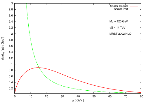
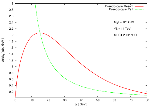
Figure 1: The transverse momentum spectrum for the scalar and pseudoscalar Higgs boson at the LHC for $|y|\leq 2.5$. The $p_{t}$ distribution peaks at approximately $15$ GeV. The resummed curve is the NLL resummation, and the perturbative curve is the NLO fixed order calculation. The NLO fixed order calculation diverges in the negative direction at small $p_{t}$. This piece of the differential cross-section is not shown for clarity. These two curves cross at approximately $p_{t}=100$ GeV/c and stay very close thereafter.

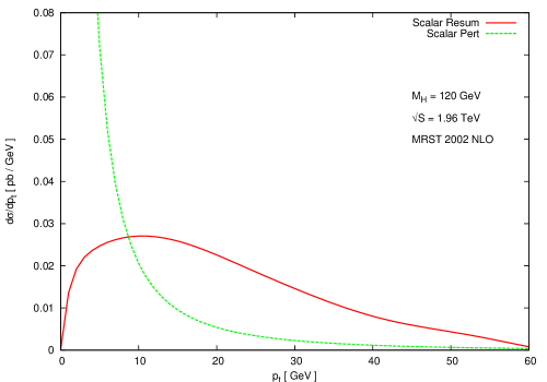
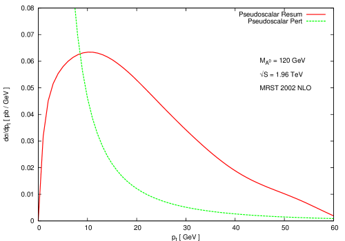
Figure 2: The transverse momentum spectrum for the scalar and pseudoscalar Higgs boson at the Tevatron for $|y|\leq 2.5$. The $p_{t}$ distribution peaks at approximately $10$ GeV. The resummed curve is the NLL resummation, and the perturbative curve is the NLO fixed order calculation. The NLO fixed order calculation diverges in the negative direction at small $p_{t}$. This piece of the differential cross-section is not shown for clarity. These two curves cross at approximately $p_{t}=80$ GeV/c and stay very close thereafter.

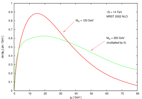
Figure 3: The effects of increasing Higgs mass on the transverse momentum spectrum at the LHC for $|y|\leq 2.5$. The $M_{H}=250$ GeV/c² curve peaks at approximately $23$ GeV/c. We can clearly see that the resummed curve peaks at higher $p_{t}$ with increasing Higgs mass and that the width of the resummed distribution becomes wider with increasing Higgs mass.

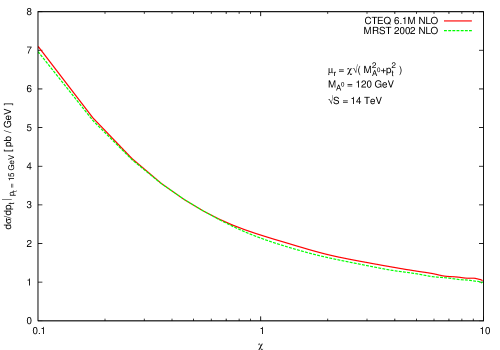
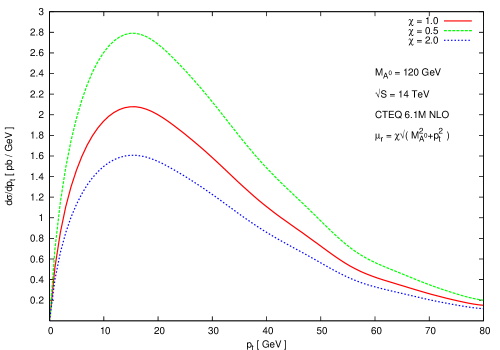
Figure 4: This is the scale uncertainty in the transverse momentum spectrum for the pseudoscalar Higgs boson. The upper figure shows the variation on the differential cross-section at its peak near $15$ GeV/c over a scale variation of an order of magnitude. The upper figure shows both the MRST and CTEQ parton distribution function. The lower figure shows the variation over the whole spectrum when the scale is varied by a factor of two. It is easy to see that the largest scale uncertainty is at the peak value.

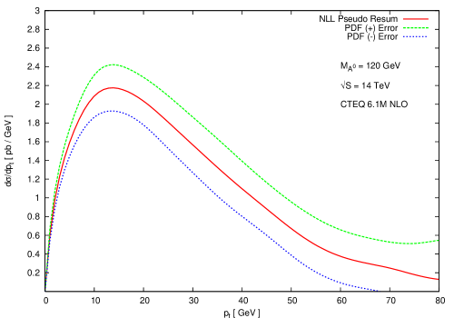
Figure 5: The uncertainty due to the parton distribution functions for the CTEQ 6.1M parton distribution functions. The resummation is done for the $gg$ initial state only and therefore has the largest PDF uncertainty. A $q\bar{q}$ initial state would have a smaller PDF uncertainty.

Although we have shown the explicit differences in the scalar and pseudoscalar functions, they are numerically quite small. Also, as the differences in the corrections become greater, they are suppressed more in $\alpha_{\textrm{s}}$, leaving the predominant difference in the resummed cross-section is the same factor of $9/4$ that appears in the LO cross-section. We are also interested in where the resummed $p_{t}$ distribution peaks at the LHC and Tevatron, so we integrated the differential cross-sections numerically for a rapidity $|y|\leq 2.5$.

We implemented the MRST2002 NLO updated parton distribution functionsMartin:2002aw ; Martin:2003sk and the MRST2001 LO parton distribution functionsMartin:2002dr in our analysis as well as the CTEQ 6.1M NLO parton distribution functionsPumplin:2002vw ; Stump:2003yu . We have taken the renormalization and factorization scales to be identical and set equal to $\mu^{2}=M_{\Phi}^{2}+p_{t}^{2}$. It should be noted that this choice of scale suppresses the width of the resummation peak as $p_{t}$ grows due to the running of the coupling constant becoming smaller as the scale increases, but the effect is not a significant one. The LO cross-section “normalization factor” in the resummation formalism also shows $p_{t}$ dependence for the same reason when this scale is used.

Our numerical results for the LHC were created with $\sqrt{S}=14$ TeV and the Tevatron with $\sqrt{S}=1.96$ TeV and a Higgs mass of $120$ GeV/c². We used an NLO one-loop $\alpha_{\textrm{s}}(M_{Z})=0.1197$ consistent with the MRST2002 NLO updated parton distribution functions and $\alpha_{\textrm{s}}(M_{Z})=0.118$ for the CTEQ 6.1M NLO parton distribution functions. The $p_{t}$ distributions for the scalar and pseudoscalar Higgs bosons at the LHC are shown in Figure 1 and Figure 2 shows the same figures for the Tevatron. It would appear that in both cases the factor of $9/4$ difference in the LO cross-sections is the dominant difference in the small $p_{t}$ region. The perturbative curves are from the same computer code that generated the differential cross-sections in Ref. Ravindran:2003um .

The average transverse momentum and transverse momentum squared at the LHC for a $120$ GeV/c² scalar and pseudoscalar Higgs boson with $p_{t}=0-80$ GeV/c are $<p_{t}>\simeq 27.5$ GeV/c and $<p_{t}^{2}>^{1/2}\simeq 32.7$ GeV/c with a peak value at $15$ GeV/c. At the Tevatron the average transverse momentum and transverse momentum squared for the scalar and pseudoscalar Higgs boson with $p_{t}=0-60$ GeV/c are $<p_{t}>\simeq 20$ GeV/c and $<p_{t}^{2}>^{1/2}\simeq 24$ GeV/c with a peak value at $10$ GeV/c. These values should be used with caution as they depend on the PDFs used in the analysis.

We are interested in what happens when a much heavier Higgs boson is considered. This would be the case if one were interested in a heavy SM Higgs, the heavy scalar $H^{0}$ in the MSSM, or a heavy pseudoscalar Higgs. We also ran our code for a Higgs with a mass of $250$ GeV/c². We found a few interesting trends. The peak in the differential distribution moved to a higher $p_{t}$ as expectedBerger:2002ut and the width of the peak became much broader. The width of the peak is interesting because it is telling us something about the decay width for the Higgs. The scale of the cross-section also dropped considerably as one would expect for a heavier final state particle. As the mass of the Higgs became very heavy, it became hard to distinguish a discernable peak in the distribution as it became very wide. As we can see in Figure 3, this is a pronounced effect. The resummed curve becomes so broad that it does not cross the fixed order differential cross-section until very high transverse momentum.

There is a great deal of interest in understanding the uncertainties associated with the differential cross-section. Although it is common to look at the scale dependence of a total cross-section for scalar Higgs productionDjouadi:2003jg , we would like to see how our results are effected by changes in the scale factor $\mu$ and the uncertainty in the parton distribution functions for the differential cross-section.

In Figure 4, the upper graph shows the scale dependence of the peak of the distribution when the scale factor is varied by a factor of ten. The lower graph in the same figure shows how the entire distribution changes when the scale is changed by a factor of two. From this lower graph is it easy to see that the peak of the distribution has the most sensitivity to the scale parameter. We define a prefactor to our renormalization scale to allow it to be varied with ease. We define $\mu^{2}=\chi^{2}(M_{\Phi}^{2}+p_{t}^{2})$. When the scale factor is changed by a factor of ten lower ($\chi=0.1$) the peak increased by a factor of approximately $3.1$ and when the scale factor is increased by a factor of ten higher ($\chi=10$) the peak of the distribution is lowered by factor of approximately $0.46$. When the scale is only varied over a more reasonable factor of two, then the peak moves by approximately $25\%$. The overall scale dependence is very close to $\alpha_{\textrm{s}}^{2}(\mu)$ running as expected from the $\sigma_{0}^{\text{LO}}$ prefactor in the resummation formalism. Overall, we can see that the shape of the distribution is not effected greatly by the change in the scale parameter, only its magnitude is changed significantly.

It is well known that the CTEQ gluon distribution is higher at small $x$ than the MRST sets which can be seen in the upper graph in Figure 4, but the effect is quite small. Otherwise, the two distributions are very similar and can be considered interchangable in this analysis.

In Figure 5, the uncertaity due to the parton distribution functions is shown. At the peak of the distribution, we see an uncertainty of approximately $10\%$. Considering only scale variations of a factor of two would lead us to believe that there is still approximately a $35\%$ uncertainty in the differential cross-section at its peak. The uncertainty would be slightly lower at other values of the transverse momentum due to the scale $\mu$ and larger at higher values of the transverse momentum due to the PDF uncertainty.

In this paper, we have calculated the resummation coefficients for pseudoscalar Higgs boson production for both the total cross-section, presenting the $B^{(2)}_{g}$, $C^{(1)}_{gg}$, and $C^{(2)}_{gg}$ coefficients, and the differential cross-section, presenting the $\bar{C}^{(1)}_{gg}$ coefficient. We have also shown the effects of increasing the mass of the Higgs boson on the resummed differential cross-section and performed an analysis of the uncertainties associated with the renormalization scale and the parton distribution functions.

Appendix A Harmonic Polynomials

Finding the Mellin moments of the fixed order total cross-section corrections has been made considerably simpler with the harmpol package in formVermaseren:2000nd . In order to use this powerful package, it is necessary to express the polylogarithmic expressions in terms of harmonic polylogarithmsVermaseren:1998uu ; Remiddi:1999ew .

Harmonic polylogarithms are defined recursively in three classes for each weight. To make this clear, let us define three functions

$$f(-1;x)=\frac{1}{1+x},\quad f(0;x)=\frac{1}{x},\quad f(1;x)=\frac{1}{1-x},$$ (50)

so we can define the weight $w=1$ harmonic polylogarithms as

$${\textrm{H}}(a;x)=\int_{0}^{x}dx^{\prime}\,f(a;x^{\prime}).$$ (51)

Thus the first three harmonic polylogarithms can be written explicitly as

$${\textrm{H}}(-1;x)=\ln(1+x),\quad{\textrm{H}}(0;x)=\ln(x),\quad{\textrm{H}}(1;x)=-\ln(1-x).$$ (52)

For higher weight harmonic polylogarithms, we need to generalize the notation. The $w$-dimensional vector $\vec{m}_{w}$ should be broken into the first index and the rest of the vector as $\vec{m}_{w}=(a,\vec{m}_{w-1})$. This gives us a general expression for the rest of the harmonic polylogarithms recursively,

$${\textrm{H}}(\vec{0}_{w};x)=\frac{1}{w!}\ln^{w}\!x,\quad{\textrm{H}}(\vec{m}_{w};x)=\int_{0}^{x}dx^{\prime}\,f(a;x^{\prime})\,{\textrm{H}}(\vec{m}_{w-1};x^{\prime}).$$ (53)

Although it is easy to find the harmonic polylogarithmic expression for the logarithms and dilogarithms, some further work is needed for the dilogarithms with quadratic arguments and the trilogarithms that appear in the NNLO corrections. The dilogarithms can be simplified in a very straightforward way using well known relationships. To list them briefly the most useful expressions are

$$-{\textrm{Li}_{2}}(1-x^{2}) =\,2[{\textrm{Li}_{2}}(x)+{\textrm{Li}_{2}}(-x)+\ln(x)\ln(1-x^{2})]-{\zeta_{2}}$$ (54)

$$-{\textrm{Li}_{2}}(1-x) =\,{\textrm{Li}_{2}}(x)+\ln(x)\ln(1-x)-{\zeta_{2}}$$ (55)

$${\textrm{Li}_{2}}(x) =\,{\textrm{H}}(0,1;x)={\textrm{H}}_{2}(x)$$ (56)

$$-{\textrm{Li}_{2}}(-x) =\,{\textrm{H}}(0,-1;x)={\textrm{H}}_{-2}(x)$$ (57)

Fewer relationships exist for the trilogarithms. It proved to be very challenging to remove three of the trilogarithmic expressions simultaneously from the NNLO corrections. The following expressions were derived from the polylogarithm literatureLewin:1958 ; Lewin:1981 and are presented here for future reference (using the notation for the Harmonic polylogarithms of Ref. Remiddi:1999ew ). That allows one to express the NNLO corrections completely in terms of Harmonic polylogarithms,

$${\textrm{Li}_{3}}\biggl{(}\frac{+(1-x)}{1+x}\biggr{)}-{\textrm{Li}_{3}}\biggl{(}\frac{-(1-x)}{1+x}\biggr{)}= \,2{\textrm{Li}_{3}}(1-x)+2{\textrm{Li}_{3}}\biggl{(}\frac{1}{1+x}\biggr{)}-\frac{1}{2}{\textrm{Li}_{3}}(1-x^{2}),$$

$$-\frac{7}{4}{\zeta_{3}}+{\zeta_{2}}\ln(1+x)-\frac{1}{3}\ln^{3}(1+x),$$ (58)

$${\textrm{Li}_{3}}\biggl{(}\frac{x}{1+x}\biggr{)}= \,\frac{1}{6}\biggl{[}\ln^{3}\biggl{(}\frac{1+x}{x}\biggr{)}+\ln^{3}(1+x)\biggr{]}-\biggl{(}\frac{{\zeta_{2}}}{2}+\frac{\ln^{2}(x)}{4}\biggr{)}\biggr{[}2\ln(1+x)-\ln(x)\biggl{]}$$

$$\quad-\frac{1}{2}\biggl{[}{\textrm{Li}_{3}}\biggl{(}-\frac{1}{x}\biggr{)}+{\textrm{Li}_{3}}(-x)\biggr{]}-{\textrm{Li}_{3}}\biggl{(}\frac{1}{1+x}\biggr{)}+{\zeta_{3}},$$ (59)

$${\textrm{Li}_{3}}\biggl{(}\frac{1}{1+x}\biggr{)}= \,\frac{1}{2}\ln^{2}(1+x)\ln(x)-\ln(1+x)\biggl{[}{\textrm{Li}_{2}}(-x)+\ln(x)\ln(1+x)-{\zeta_{2}}\biggr{]}+{\zeta_{2}}$$

$$-{\textrm{H}}_{-2,-1}(x)+{\zeta_{2}}\ln(1+x)+\frac{1}{6}\biggl{[}\ln^{3}(1+x)-18{\zeta_{2}}\ln(1+x)\biggr{]},$$ (60)

$${\textrm{Li}_{3}}\biggl{(}\frac{-(1-x)}{x}\biggr{)}= \,-{\textrm{Li}_{3}}(1-x)-{\textrm{Li}_{3}}(x)+{\zeta_{3}}+{\zeta_{2}}\ln(1-x)-\frac{1}{2}\ln(x)\ln^{2}(1-x)+\frac{1}{6}\ln^{3}(1-x)$$

$$-{\zeta_{2}}\ln\biggl{(}\frac{1-x}{x}\biggr{)}-\frac{1}{6}\ln^{3}\biggl{(}\frac{1-x}{x}\biggr{)},$$ (61)

$${\textrm{Li}_{3}}\biggl{(}\frac{-(1-x^{2})}{x^{2}}\biggr{)}= \,-{\textrm{Li}_{3}}(1-x^{2})-4\biggl{[}{\textrm{Li}_{3}}(x)+{\textrm{Li}_{3}}(-x)\biggr{]}+{\zeta_{3}}+{\zeta_{2}}\ln(1-x^{2})$$

$$-\ln(x)\ln^{2}(1-x^{2})+\frac{1}{6}\ln^{3}(1-x^{2})-{\zeta_{2}}\ln\biggl{(}\frac{1-x^{2}}{x^{2}}\biggr{)}-\frac{1}{6}\ln^{3}\biggl{(}\frac{1-x^{2}}{x^{2}}\biggr{)},$$ (62)

$${\textrm{Li}_{3}}(1-x^{2})= \,\ln(x)\ln^{2}(1-x^{2})+{\textrm{Li}_{2}}(1-x^{2})\ln(1-x^{2})+{\zeta_{3}}-2\biggl{[}{\textrm{H}}_{2,1}(x)-{\textrm{H}}_{-2,1}(x)\biggr{]},$$ (63)

$${\textrm{Li}_{3}}(1-x)= \,\frac{1}{2}\ln(x)\ln^{2}(1-x)+\ln(1-x){\textrm{Li}_{2}}(1-x)+{\zeta_{3}}-{\textrm{H}}_{2,1}(x),$$ (64)

$${\textrm{Li}_{3}}\biggl{(}-\frac{1}{x}\biggr{)}= \,{\textrm{Li}_{3}}(-x)+{\zeta_{2}}\ln(x)+\frac{1}{6}\ln^{3}(x),$$ (65)

$${\textrm{Li}_{3}}(x)= \,{\textrm{H}}_{3}(x),$$ (66)

$$-{\textrm{Li}_{3}}(-x)= \,{\textrm{H}}_{-3}(x),$$ (67)

$$-S_{1,2}(1-x)= \,{\textrm{Li}_{3}}(x)+\ln(x){\textrm{Li}_{2}}(x)+\frac{1}{2}\ln(1-x)\ln^{2}(x)+{\zeta_{3}},$$ (68)

$$-S_{1,2}(-x)= \,{\textrm{H}}_{-2,-1}(x).$$ (69)

It was also necessary to linearize all the arguments of the natural logs and to partial fraction the inverse powers of $1-x^{2}$. With these above expressions, it was possible to use harmpol to find the Mellin moments of the correction factors. Although most of these expressions were verified numerically, it should be emphasized that these expressions were derived so that they would be valid at $x\leq 1$, which is where they would be evaluated on threshold. In some regions these expressions would pick up imaginary pieces, but since we are interested in corrections to a partonic cross-section our expression must stay real.

Using these expressions, the NNLO corrections in Refs. Harlander:2001is ; Harlander:2002vv ; Ravindran:2003um can be reduced to Harmonic polylogarithms so their moments can be easily found.

References

• (1) J. F. Gunion, H. E. Haber, G. L. Kane and S. Dawson, β€œThe Higgs Hunter’s Guide”, (Addison-Wesley, Reading, MA, 1990), Erratum ibid. [arXiv:hep-ph/9302272].
• (2) M. Carena and H. E. Haber, Prog. Part. Nucl. Phys.  50, 63 (2003) [arXiv:hep-ph/0208209].
• (3) Tevatron Electroweak Working Group [D0 Collaboration], arXiv:hep-ex/0404010.
• (4) R. Barate et al. [ALEPH Collaboration], Phys. Lett. B 565, 61 (2003) [arXiv:hep-ex/0306033].
• (5) J. Fernandez [DELPHI Collaboration], eConf C030626, FRAP09 (2003) [arXiv:hep-ex/0307002].
• (6) S. Catani and L. Trentadue, Nucl. Phys. B 327, 323 (1989).
• (7) R. P. Kauffman, Phys. Rev. D 44, 1415 (1991).
• (8) C. P. Yuan, Phys. Lett. B 283, 395 (1992).
• (9) R. P. Kauffman, Phys. Rev. D 45, 1512 (1992).
• (10) S. Catani, M. L. Mangano, P. Nason and L. Trentadue, Nucl. Phys. B 478, 273 (1996) [arXiv:hep-ph/9604351].
• (11) M. Kramer, E. Laenen and M. Spira, Nucl. Phys. B 511, 523 (1998)
• (12) C. Balazs and C. P. Yuan, Phys. Lett. B 478, 192 (2000) [arXiv:hep-ph/0001103].
• (13) D. de Florian and M. Grazzini, Phys. Rev. Lett.  85, 4678 (2000) [arXiv:hep-ph/0008152].
• (14) D. de Florian and M. Grazzini, Nucl. Phys. B 616, 247 (2001) [arXiv:hep-ph/0108273].
• (15) C. J. Glosser and C. R. Schmidt, JHEP 0212, 016 (2002) [arXiv:hep-ph/0209248].
• (16) E. L. Berger and J.-w. Qiu, Phys. Rev. D 67, 034026 (2003) [arXiv:hep-ph/0210135].
• (17) E. L. Berger and J.-w. Qiu, Phys. Rev. Lett.  91, 222003 (2003) [arXiv:hep-ph/0304267].
• (18) G. Bozzi, S. Catani, D. de Florian and M. Grazzini, Phys. Lett. B 564, 65 (2003) [arXiv:hep-ph/0302104].
• (19) S. Catani, D. de Florian, M. Grazzini and P. Nason, JHEP 0307, 028 (2003) [arXiv:hep-ph/0306211].
• (20) A. Kulesza, G. Sterman and W. Vogelsang, Phys. Rev. D 69, 014012 (2004) [arXiv:hep-ph/0309264].
• (21) R. V. Harlander and W. B. Kilgore, Phys. Rev. D 68, 013001 (2003) [arXiv:hep-ph/0304035].
• (22) B. Field, S. Dawson and J. Smith, Phys. Rev. D 69, 074013 (2004) [arXiv:hep-ph/0311199].
• (23) F. Wilczek, Phys. Rev. Lett.  39, 1304 (1977).
• (24) J. R. Ellis, M. K. Gaillard, D. V. Nanopoulos and C. T. Sachrajda, Phys. Lett. B 83, 339 (1979).
• (25) H. M. Georgi, S. L. Glashow, M. E. Machacek and D. V. Nanopoulos, Collisions,” Phys. Rev. Lett.  40, 692 (1978).
• (26) T. G. Rizzo, Phys. Rev. D 22, 178 (1980) [Addendum-ibid. D 22, 1824 (1980)].
• (27) M. A. Shifman, A. I. Vainshtein, M. B. Voloshin and V. I. Zakharov, Sov. J. Nucl. Phys.  30, 711 (1979) [Yad. Fiz.  30, 1368 (1979)].
• (28) A. I. Vainshtein, V. I. Zakharov and M. A. Shifman, Sov. Phys. Usp.  23, 429 (1980) [Usp. Fiz. Nauk 131, 537 (1980)].
• (29) M. B. Voloshin, Sov. J. Nucl. Phys.  45, 122 (1987) [Yad. Fiz.  45, 190 (1987)].
• (30) K. G. Chetyrkin, B. A. Kniehl and M. Steinhauser, Phys. Rev. Lett.  79, 2184 (1997) [arXiv:hep-ph/9706430].
• (31) R. P. Kauffman, S. V. Desai and D. Risal, Phys. Rev. D 55, 4005 (1997) [Erratum-ibid. D 58, 119901 (1998)] [arXiv:hep-ph/9610541]. Further typos corrected in Ravindran:2002dc .
• (32) K. G. Chetyrkin, B. A. Kniehl, M. Steinhauser and W. A. Bardeen, Nucl. Phys. B 535, 3 (1998) [arXiv:hep-ph/9807241].
• (33) R. P. Kauffman and W. Schaffer, Phys. Rev. D 49, 551 (1994) [arXiv:hep-ph/9305279].
• (34) R. V. Harlander and W. B. Kilgore, Phys. Rev. D 64, 013015 (2001) [arXiv:hep-ph/0102241].
• (35) R. V. Harlander and W. B. Kilgore, JHEP 0210, 017 (2002) [arXiv:hep-ph/0208096].
• (36) V. Ravindran, J. Smith and W. L. van Neerven, Nucl. Phys. B 665, 325 (2003) [arXiv:hep-ph/0302135].
• (37) S. Dawson, Nucl. Phys. B 359, 283 (1991).
• (38) A. Djouadi, M. Spira and P. M. Zerwas, Phys. Lett. B 264, 440 (1991).
• (39) M. Spira, A. Djouadi, D. Graudenz and P. M. Zerwas, Nucl. Phys. B 453, 17 (1995) [arXiv:hep-ph/9504378].
• (40) V. Ravindran, J. Smith and W. L. Van Neerven, Nucl. Phys. B 634, 247 (2002) [arXiv:hep-ph/0201114].
• (41) B. Field, J. Smith, M. E. Tejeda-Yeomans and W. L. van Neerven, Phys. Lett. B 551, 137 (2003) [arXiv:hep-ph/0210369].
• (42) R. K. Ellis, I. Hinchliffe, M. Soldate and J. J. van der Bij, Nucl. Phys. B 297, 221 (1988).
• (43) U. Baur and E. W. N. Glover, Nucl. Phys. B 339, 38 (1990).
• (44) G. β€™t Hooft and M. J. G. Veltman, Nucl. Phys. B 44, 189 (1972).
• (45) D. A. Akyeampong and R. Delbourgo, Nuovo Cim. A 17, 578 (1973).
• (46) D. A. Akyeampong and R. Delbourgo, Nuovo Cim. A 18, 94 (1973).
• (47) D. A. Akyeampong and R. Delbourgo, Nuovo Cim. A 19, 219 (1974).
• (48) J. C. Collins and D. E. Soper, Nucl. Phys. B 193, 381 (1981) [Erratum-ibid. B 213, 545 (1983)].
• (49) J. C. Collins and D. E. Soper, Nucl. Phys. B 197, 446 (1982).
• (50) J. C. Collins, D. E. Soper and G. Sterman, Nucl. Phys. B 250, 199 (1985).
• (51) P. B. Arnold and R. P. Kauffman, Nucl. Phys. B 349, 381 (1991).
• (52) C. T. H. Davies and W. J. Stirling, Nucl. Phys. B 244, 337 (1984).
• (53) A. Vogt, S. Moch and J. A. M. Vermaseren, arXiv:hep-ph/0404111.
• (54) S. Moch, J. A. M. Vermaseren and A. Vogt, Nucl. Phys. B 688, 101 (2004) [arXiv:hep-ph/0403192].
• (55) A. Vogt, Phys. Lett. B 497, 228 (2001) [arXiv:hep-ph/0010146].
• (56) J. A. M. Vermaseren, arXiv:math-ph/0010025.
• (57) A. D. Martin, R. G. Roberts, W. J. Stirling and R. S. Thorne, Eur. Phys. J. C 28, 455 (2003) [arXiv:hep-ph/0211080].
• (58) A. D. Martin, R. G. Roberts, W. J. Stirling and R. S. Thorne, arXiv:hep-ph/0308087.
• (59) A. D. Martin, R. G. Roberts, W. J. Stirling and R. S. Thorne, Phys. Lett. B 531, 216 (2002) [arXiv:hep-ph/0201127].
• (60) J. Pumplin, D. R. Stump, J. Huston, H. L. Lai, P. Nadolsky and W. K. Tung, JHEP 0207, 012 (2002) [arXiv:hep-ph/0201195].
• (61) D. Stump, J. Huston, J. Pumplin, W. K. Tung, H. L. Lai, S. Kuhlmann and J. F. Owens, JHEP 0310, 046 (2003) [arXiv:hep-ph/0303013].
• (62) A. Djouadi and S. Ferrag, Phys. Lett. B 586, 345 (2004) [arXiv:hep-ph/0310209].
• (63) J. A. M. Vermaseren, Int. J. Mod. Phys. A 14, 2037 (1999) [arXiv:hep-ph/9806280].
• (64) E. Remiddi and J. A. M. Vermaseren, Int. J. Mod. Phys. A 15, 725 (2000) [arXiv:hep-ph/9905237].
• (65) L. Lewin, β€œDilogarithms and Associated Functions”, (North Holland, 1958).
• (66) L. Lewin, β€œPolylogarithms and Associated Functions”, (North Holland, 1981).