Comparison of numerical solutions for $Q^{2}$ evolution equations

Abstract

$Q^{2}$ evolution equations are important not only for describing hadron reactions in accelerator experiments but also for investigating ultrahigh-energy cosmic rays. The standard ones are called DGLAP evolution equations, which are integrodifferential equations. There are methods for solving the $Q^{2}$ evolution equations for parton-distribution and fragmentation functions. Because the equations cannot be solved analytically, various methods have been developed for the numerical solution. We compare brute-force, Laguerre-polynomial, and Mellin-transformation methods particularly by focusing on the numerical accuracy and computational efficiency. An efficient solution could be used, for example, in the studies of a top-down scenario for the ultrahigh-energy cosmic rays.

SAGA-HE-199-04

1 Introduction

High-energy hadron reactions are described in terms of parton-distribution functions (PDFs) and fragmentation functions (FFs). There are parametrizations for the PDFs [1] and FFs [2]. Using these functions, cross sections of high-energy hadron reactions are evaluated. Precise calculations of these cross sections are important for finding any new physics beyond the current theoretical framework.

The PDFs depend on two kinematical variables $x$ and $Q^{2}$. They are defined by $Q^{2}=-q^{2}$ and $x=Q^{2}/(2p\cdot q)$ in lepton scattering with the momentum transfer $q$ and the hadron momentum $p$. The FFs depend on $Q^{2}$ and another variable $x=2E_{h}/\sqrt{s}$, where $E_{h}$ is the hadron energy and $\sqrt{s}$ is the center-of-mass energy. Their $Q^{2}$ dependence is called scaling violation, which is calculated by the DGLAP (Dokshitzer-Gribov-Lipatov-Altarelli-Parisi) evolution equations [3] in the perturbative QCD region.

The $Q^{2}$ evolution equations are frequently used in describing high-energy hadron reactions. Because the PDFs and FFs vary significantly in the current accelerator-reaction range, $Q^{2}$=1 GeV² to 10⁵ GeV², the $Q^{2}$ dependence should be calculated accurately. Furthermore, it is known that high-energy cosmic rays have energies much more than the TeV scale. Analytical forms of current PDFs and FFs are supplied typically in the GeV region, so that they have to be evolved to the scale which could be more than TeV in order to use them for investigating the cosmic rays [4, 5].

A useful evolution code was developed in Ref. [4] for the cosmic ray studies. The Laguerre-polynomial method was used for solving the evolution equations. Splitting functions, PDFs, and FFs are expanded in terms of the Laguerre polynomials, and then the evolution is described by a simple summation of their expansion coefficients. In fact, the method is very efficient for solving the equations in comparison, for example, with a direct integration method [6, 7]. However, because the Laguerre polynomials $L_{n}(-\ln x)$ go to infinity in the limit $x\rightarrow 0$, it could have an accuracy problem in the small $x$ region where high-energy reactions are sensitive. In this paper, we discuss evolution results by the Laguerre method [4, 8] in comparison with the ones by other solution methods, “brute-force” [6] and Mellin-transformation [9] methods. In particular, evolution accuracy and computation time are compared. It is the purpose of this paper to clarify the advantages and disadvantages of these numerical solution methods for a better description of high-energy hadron reactions including the high-energy cosmic rays. In particular, the FF evolution could be used for studying a top-down scenario in order to determine the origin of ultrahigh-energy cosmic rays, namely from a decay of a superheavy particle [5].

This paper consists of the following. The DGLAP evolution equations are introduced in Sec. 2, and numerical solution methods are explained in Sec. 3. Evolution results and their comparisons are discussed in Sec. 4. The results are summarized in Sec. 5.

2 $Q^{2}$ evolution equations

From the cross-section measurements of high-energy lepton-hadron, hadron-hadron, and lepton-annihilation reactions, the PDFs and FFs are extracted. The PDFs and FFs are expressed in terms of the two kinematical variables $x$ and $Q^{2}$. A PDF or a FF is expressed $f(x,Q^{2})$ in the following. We investigate the standard $Q^{2}$ evolution equations, which are called the DGLAP evolution equations [3]. The flavor nonsinglet equation is written as

$$\frac{\partial}{\partial\ln Q^{2}}\ f_{{}_{NS}}(x,Q^{2})=\frac{\alpha_{s}(Q^{2})}{2\pi}\,\int_{x}^{1}\frac{dy}{y}\,P_{{}_{NS}}(x/y)\,f_{{}_{NS}}(y,Q^{2}),$$ (1)

where $f_{{}_{NS}}(x,Q^{2})$ is a nonsinglet (NS) function, $P_{{}_{NS}}(x)$ is a nonsinglet splitting function, and $\alpha_{s}(Q^{2})$ is the running coupling constant. The splitting functions for parton distributions and fragmentation functions are identical in the leading order (LO) of $\alpha_{s}$; however, they differ if higher order corrections are included [10]. In order to make the evolution equation slightly simpler, the variable $t$ is used instead of $Q^{2}$:

$$t\equiv-\frac{2}{\beta_{0}}\ln\biggl{[}\frac{\alpha_{s}(Q^{2})}{\alpha_{s}(Q_{0}^{2})}\biggr{]},$$ (2)

where the running coupling constant in the leading order (LO) is given by $\alpha_{s}(Q^{2})=4\pi/[\beta_{0}\ln(Q^{2}/\Lambda^{2})]$ with the QCD scale parameter $\Lambda$. The constant $\beta_{0}$ is expressed as $\beta_{0}=11C_{G}/3-4T_{R}N_{f}/3$ with $C_{G}=N_{c}$ and $T_{R}=1/2$. Here, $N_{c}$ is the number of color ($N_{c}$=3) and $N_{f}$ is the number of flavor. The $Q_{0}^{2}$ in Eq. (2) indicates the initial $Q^{2}$ where the evolved function is provided. Using this variable $t$ in Eq. (1), we obtain

$$\frac{\partial}{\partial t}\,f_{{}_{NS}}(x,t)=\int_{x}^{1}\frac{dy}{y}\,P_{{}_{NS}}(x/y)\,f_{{}_{NS}}(y,t),$$ (3)

for the nonsinglet evolution.

In the flavor singlet case, the evolution is described by two coupled integrodifferential equations:

$$\frac{\partial}{\partial t}\,{\bf f}(x,t)=\int_{x}^{1}\,\frac{dy}{y}\,{\bf P}(x/y)\,{\bf f}(y,t),$$ (4)

where the matrices ${\bf f}$ and ${\bf P}$ are defined by

$${\bf f}(x,t)=\begin{pmatrix}f_{{}_{S}}(x,t)\\ f_{g}(x,t)\end{pmatrix},\ \ \ \ {\bf P}(x)=\begin{pmatrix}P_{qq}(x)&2N_{f}P_{ij}(x)\\ P_{ji}(x)&P_{gg}(x)\end{pmatrix}.$$ (5)

The indices $i$ and $j$ indicate $ij=qg$ for the PDFs and $ij=gq$ for the FFs. The functions $P_{qq}$, $P_{qg}$, $P_{gq}$, and $P_{gg}$ are splitting functions. The function $P_{ij}$ determines the probability of the splitting process that a parton $j$ with the momentum fraction $y$ splits into a parton $i$ with the momentum fraction $x$ and another parton and the $j$-parton momentum is reduced by the fraction $z$. In the LO, the splitting functions are expressed as

$$P_{qq}(x)= P_{{}_{NS}}(x)=C_{F}\,\left[\,\frac{1+x^{2}}{(1-x)_{+}}+\frac{3}{2}\,\delta(1-x)\,\right],$$

$$P_{qg}(x)= T_{R}\left[\,x^{2}+(1-x)^{2}\ \right],$$

$$P_{gq}(x)= C_{F}\ \frac{1+(1-x)^{2}}{x},$$ (6)

$$P_{gg}(x)= 2\,C_{G}\left[\,\frac{x}{(1-x)_{+}}+\frac{1-x}{x}\ +\ x(1-x)+\left(\frac{11}{12}-\frac{1}{3}\frac{N_{f}T_{R}}{C_{G}}\right)\,\delta(1-x)\,\right],$$

where $C_{F}$ is given by $C_{F}=(N_{c}^{2}-1)/(2N_{c})$ and $1/(1-x)_{+}$ is defined by $\int_{0}^{1}dx\,g(x)/(1-x)_{+}=\int_{0}^{1}dx\,[g(x)-g(1)]/(1-x)$ with an arbitrary function $g(x)$.

We need to solve the nonsinglet and singlet evolution equations in Eqs. (3) and (4). These are not simple integrodifferential equations, so that an efficient numerical method should be investigated. In the next section, three popular numerical methods are explained.

3 Numerical Methods for solving $Q^{2}$ evolution equations

There are various ways for solving the DGLAP equations. In this section, we explain three popular methods, brute-force, Laguerre-polynomial, and Mellin-transformation methods. In the following subsections, only the nonsinglet evolution is explained because the singlet evolution can be solved in the same way.

3.1 Brute-force method

The simplest way is possibly to use the brute-force method [6, 7]. It may seem to be too simple, but it is especially suitable for solving more complicated equations with higher-twist terms [11]. These equations could not be easily handled by the orthogonal-polynomial methods such as the Laguerre-polynomial one in Sec. 3.2 and by the Mellin-transformation method in Sec. 3.3. Furthermore, a computer code is so simple that the possibility of a program mistake is small, which means the code could be used for checking other numerical methods. These are the reasons why it was investigated in Ref. [7].

In the brute-force method, the two variables $t$ and $x$ are divided into small steps, and then the differentiation and integration are defined by

$$\frac{\partial f(x,t)}{\partial t}\Rightarrow\frac{f(x_{i},t_{j+1})-f(x_{i},t_{j})}{\Delta t_{j}},\ \ \ \ \int dxf(x,t)\Rightarrow\sum_{k=1}^{N_{x}}\Delta x_{k}f(x_{k},t_{j}),$$ (7)

where $\Delta t_{j}$ and $\Delta x_{k}$ are the steps at the positions $j$ and $k$, and they are given by $\Delta t_{j}=t_{j+1}-t_{j}$ and $\Delta x_{k}=x_{k}-x_{k-1}$. The numbers of $t$ and $x$ steps are denoted $N_{t}$ and $N_{x}$, respectively. Applying these equations to Eq. (3), we write the nonsinglet evolution from $t_{j}$ to $t_{j+1}$ as

$$q_{{}_{NS}}(x_{i},t_{j+1})=q_{{}_{NS}}(x_{i},t_{j})+\Delta t_{j}\sum_{k=i}^{N_{x}}\frac{\Delta x_{k}}{x_{k}}P_{qq}(x_{i}/x_{k})q_{{}_{NS}}(x_{k},t_{j}).$$ (8)

If the distribution $q_{{}_{NS}}$ is supplied at $t_{1}=0$, the next one $q_{{}_{NS}}(x,t_{2})$ can be calculated by the above equation. Repeating this step $N_{t}-1$ times, we obtain the final distribution at $t_{N_{t}}$. However, it is obvious that the step numbers $N_{t}$ and $N_{x}$ should be large enough to obtain an accurate evolution result.

3.2 Laguerre polynomial method

The evolution equations could be solved by expanding the distribution and splitting functions in terms of orthogonal polynomials. A popular method of this type is to use the Laguerre polynomials [4, 8]. They are defined in the region from 0 to $\infty$, so that the variable $x$ should be transformed to $x^{\prime}$ by the relation $x^{\prime}=-\ln\,x$.

The nonsinglet evolution is discussed in the following. The evolution function $E_{{}_{NS}}(x,t)$, which describes the distribution evolution from $t=0$ to $t$, is defined by

$$f_{{}_{NS}}(x,t)=\int_{x}^{1}\frac{dy}{y}\,E_{{}_{NS}}(x/y,t)\,f_{{}_{NS}}(y,t=0).$$ (9)

Then, it satisfies

$$\frac{\partial}{\partial t}\,E_{{}_{NS}}(x,t)=\int_{x}^{1}\frac{dy}{y}\,P_{{}_{NS}}(x/y)\,E_{{}_{NS}}(y,t).$$ (10)

Because this is the same integrodifferential equation as the original DGLAP equation, one may wonder why such a function should be introduced. There is an advantage that the evolution function should be the delta function at $t=0$: $E_{{}_{NS}}(x,t=0)=\delta(1-x)$ because of its definition in Eq. (9). It makes the following analysis simpler. The functions are expanded in terms of the polynomials: $P_{{}_{NS}}(e^{-x^{\prime}})=\sum_{n}P_{{}_{NS}}^{n}L_{n}(x^{\prime})$ and $E_{{}_{NS}}(e^{-x^{\prime}},t)=\sum_{n}E_{{}_{NS}}^{n}(t)L_{n}(x^{\prime})$, where $P_{{}_{NS}}^{n}$ and $E_{{}_{NS}}^{n}(t)$ are the expansion coefficients. The coefficient $F^{n}$ for a function $F(x)$ is given by $F^{n}=\int_{0}^{1}dxL_{n}(x^{\prime})\,F(x)$, and it could be calculated analytically for a simple function. If the two functions on the right-hand side of Eq. (10) are expanded, it becomes an integration of two Laguerre polynomials. Using the formula $\int_{0}^{x^{\prime}}dy^{\prime}L_{n}(x^{\prime}-y^{\prime})L_{m}(y^{\prime})=L_{n+m}(x^{\prime})-L_{n+m+1}(x^{\prime})$ for this integration, we obtain

$$\frac{d}{dt}\,E_{{}_{NS}}^{n}(t)=\sum_{m=0}^{n}(P_{{}_{NS}}^{n-m}-P_{{}_{NS}}^{n-m-1})\,E_{m}(t).$$ (11)

Because the evolution function is a delta function at $t=0$, all the expansion coefficients are one. Therefore, this equation is easily solved to give a summation form:

$$E_{{}_{NS}}^{m}(t)=e^{P_{{}_{NS}}^{0}t}\sum_{k=0}^{m}\frac{t^{k}}{k!}\,B_{m}^{k},\ \ \ B_{m}^{k+1}=\sum_{i=k}^{m-1}(P_{{}_{NS}}^{m-i}-P_{{}_{NS}}^{m-i-1})B_{i}^{k}.$$ (12)

This recursion relation is calculated with the relations $B_{i}^{0}=1$, $B_{i}^{1}=\!\sum_{j=1}^{i}(P_{{}_{NS}}^{j}-P_{{}_{NS}}^{j-1})$, and $B_{0}^{k}=B_{1}^{k}=\cdots=B_{k-1}^{k}=0$. After all, the evolution is calculated by the simple summation:

$$f_{{}_{NS}}(x,t)=\sum_{n=0}^{N_{Lag}}\sum_{m=0}^{n}\,[E_{n-m}(t)-E_{n-m-1}(t)]\,L_{n}(-\ln\,x)f_{{}_{NS}}^{\ m}(t=0).$$ (13)

In this way, the integrodifferential equation becomes a simple summation of Laguerre-expansion coefficients, so that this method is considered to be a very efficient numerical method for the solution.

3.3 Mellin transformation method

The Mellin transformation method is one of the popular evolution methods [9]. It is used because the Mellin transformation of the right-hand side of Eq. (3) becomes a simple multiplication of two moments, namely the moments of the splitting function and the distribution function. The moments of the splitting functions (anomalous dimensions) are well known, and a simple functional form is usually assumed for the distribution at certain small $Q^{2}$ so as to calculate its moments easily. Then, it is straightforward to obtain the analytical solution in the moment space. Furthermore, the computation time is fairly short. These are the reasons why this method has been used as a popular method. For example, it is used for the $\chi^{2}$ analysis of experimental data for obtaining polarized PDFs [12], whereas the brute-force method is employed in Ref. [13].

The Mellin transformation and inversion are defined by

$$\hat{f}(s,t)=\int_{0}^{1}dx\,x^{s-1}\,f(x,t),\ \ \ \ f(x,t)=\frac{1}{2\pi i}\int_{c-i\infty}^{c+i\infty}ds\,x^{-s}\,\hat{f}(s,t).$$ (14)

Here, the upper limit of the $x$ integration is taken one because the distribution $f(x)$ vanishes in the region $x\geq 1$. The Mellin inversion is a complex integral with an arbitrary real constant $c$, which should be taken so that the integral $\int_{0}^{1}dxf(x)x^{c-1}$ is absolutely convergent. If this transformation is used, the integrodifferential equations become very simple. For example, the nonsinglet evolution equation becomes

$$\frac{\partial}{\partial t}\,\hat{f}_{{}_{NS}}(s,t)=\hat{P}_{{}_{NS}}(s)\,\hat{f}_{{}_{NS}}(s,t).$$ (15)

Its solution is simply given by

$$\hat{f}_{{}_{NS}}(s,t)=e^{\hat{P}_{{}_{NS}}(s)\,t}\ \hat{f}_{{}_{NS}}(s,t=0).$$ (16)

Figure 1: Integration contour.

Because the moments $\hat{P}_{{}_{NS}}(s)$ are well known quantities and the moments of the initial function $\hat{f}_{{}_{NS}}(s,t=0)$ could be evaluated, it is straightforward to calculate the evolution in Eq. (16) in the moment space. However, the numerical integration is needed for the Mellin inversion in Eq. (14) for transforming the moments into a corresponding $x$ distribution. Practically, the Mellin inversion is calculated along the integration contour in Fig. 1. Changing the complex integration variable $s$ for the real one $z$ by $s=c+ze^{i\phi}$ in Eq. (14), we have

$$f_{{}_{NS}}(x,t)=\frac{1}{\pi}\int_{0}^{\infty}dz\,Im\left[e^{i\phi}\,x^{-c-ze^{i\phi}}\,\hat{f}_{{}_{NS}}(s=c+ze^{i\phi},t)\right].$$ (17)

The constant $c$ and the angle $\phi$ are shown in Fig. 1. Using the Gauss-Legendre quadrature for this integration, we obtain the evolved distribution in the $x$ space.

4 Comparison of evolution results

In comparing evolution results of three methods, we take the evolved distribution of the brute-force (BF) method with $N_{t}$=200 and $N_{x}$=4000 as a standard for assessing other evolution accuracy. It is shown in Ref. [7] that the evolution accuracy is better than 2% if $N_{t}$=200 and $N_{x}$=1000 are taken. This is the reason why it is taken as the standard. Because the details are discussed in Ref. [7] for the evolution accuracy of the BF method, we discuss only the comparison with the results of the Laguerre-polynomial and Mellin-transformation methods.

4.1 Parton distribution functions

In order to show the $Q^{2}$ evolution of the PDFs, we use the MRST02 distributions [14] which are provided analytically at $Q^{2}$=1 GeV². The distributions are evolved to $Q^{2}$=100 GeV² with the MRST02 scale parameter by three evolution methods. Then, the ratio of the evolved distribution to the one by the brute-force method with $N_{t}$=200 and $N_{x}$=4000 is shown for finding the numerical accuracy.

First, the evolution results of the nonsinglet distribution $x(u_{v}+d_{v})$ are shown in Fig. 3 for the Laguerre method. The number of the Laguerre polynomials $N_{Lag}$ is taken as $N_{Lag}$=5, 10, 20, and 30, and each distribution ratio $x(u_{v}+d_{v})_{Laguerre}/x(u_{v}+d_{v})_{BF(N_{t}=200,N_{x}=4000)}$ is shown. It is obvious that accurate evolution cannot be obtained if the number $N_{Lag}$ is small in the small- and large-$x$ regions. In particular, the ratio shows oscillatory behavior at small $x$, which results from the functional behavior of the Laguerre polynomials. The Laguerre polynomials $L_{n}(-\ln\,x)$ are shown as a function of $x$ in Fig. 3. We find that the oscillatory functional form at small $x$ gives rise to the oscillatory behavior in Fig. 3. Therefore, one should be careful in the Laguerre method that a large number of polynomials should be taken to obtain an accurate evolution at small $x$. Furthermore, one should be also careful in the very-large-$x$ region.

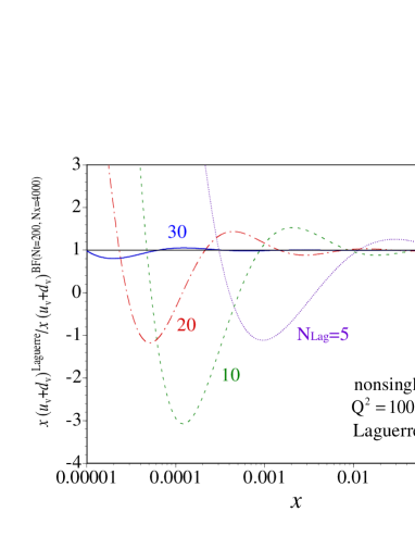
Figure 2: Evolved nonsinglet distribution ratios $x(u_{v}+d_{v})^{Laguerre}/x(u_{v}+d_{v})^{BF}$ are shown for $N_{Lag}$=5, 10, 20, and 30 in the Laguerre-polynomial method.

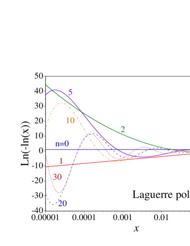
Figure 3: Laguerre polynomials $L_{n}(-\ln x)$.

Next, the evolution results are shown in Fig. 5 for the Mellin-transformation method. The Mellin inversion of Eq. (17) is numerically calculated by the Gauss-Legendre quadrature with the number of points $N_{GL}$, which is taken as $N_{GL}$=6, 10, 20, and 50 in Fig. 5. The integration contour of Fig. 1 is used with the constants $c$=1.1 and $\phi$=135^∘ as suggested in Ref. [9]. In order to use the Gauss-Legendre quadrature, the upper limit of the integration of Eq. (17) should be assigned. We decided to take $z_{max}=16.5x+3.5$ so that the integrand is small enough at $z=z_{max}$ for the $x$ region $10^{-5}<x<0.99$. If the number $N_{GL}$ is small, the evolved nonsinglet distribution is not accurate enough in the small and large $x$ regions as shown in Fig. 5.

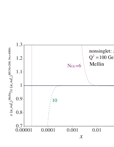
Figure 4: Evolved nonsinglet distribution ratios $x(u_{v}+d_{v})^{Mellin}/x(u_{v}+d_{v})^{BF}$ are shown for $N_{GL}$=6, 10, 20, and 50 in the Mellin-transformation method.

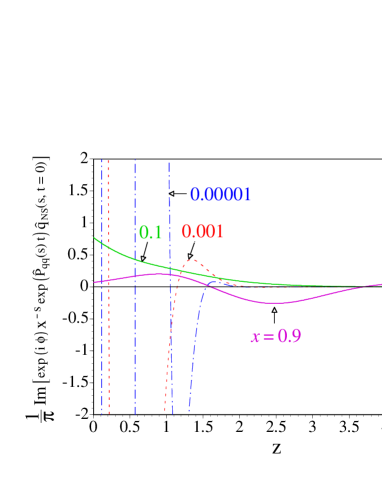
Figure 5: Integrand of the Mellin inversion in Eq. (17).

The inaccuracy in the small and large $x$ regions for $N_{GL}$=6 and 10 is understood in the following way. We show the integrand of Eq. (17) in Fig. 5 by taking $x$=$10^{-5}$, $10^{-3}$, $10^{-1}$, and 0.9. It is clear that the integrand oscillates at small $x$ so that a certain number of Gauss-Legendre points is needed for getting an accurate evolution. On the other hand, the integrand does not decrease rapidly at large $z$ for the large-$x$ case ($x$=0.9), so that large $z_{max}$ should be taken for the integration. In addition, the positive contribution at $z\sim 1$ and the negative one at $z\sim 2.5$ almost cancel each other, which is another source of numerical inaccuracy.

The evolution results of the singlet distribution are shown in Figs. 7 and 7 for the Laguerre and Mellin methods, respectively. We notice in Fig. 7 that the accuracy of the singlet evolution is much better than the nonsinglet one in the Laguerre method. It comes simply from the functional difference between the nonsinglet and singlet distributions. The Laguerre method can be used as an accurate evolution method for the singlet evolution. The singlet evolution accuracy for the Mellin method is similar to its nonsinglet ones. If the point number $N_{GL}$ is large enough, the evolution becomes accurate.

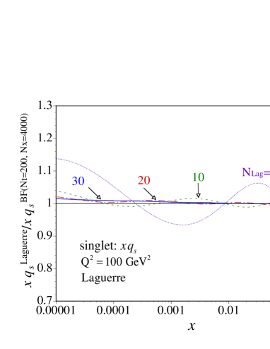
Figure 6: Evolved singlet distribution ratios $xq_{s}^{Laguerre}/xq_{s}^{BF}$ are shown for $N_{Lag}$=5, 10, 20, and 30 in the Laguerre-polynomial method.

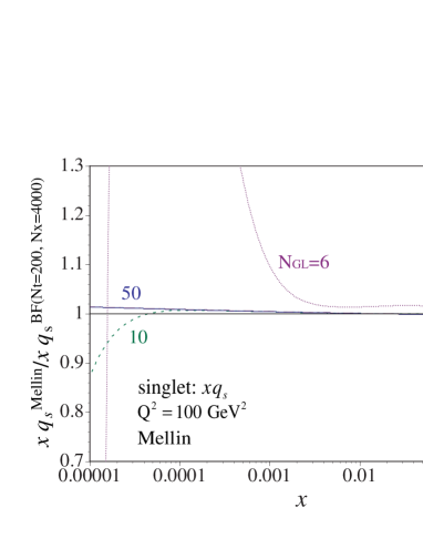
Figure 7: Evolved singlet distribution ratios $xq_{s}^{Mellin}/xq_{s}^{BF}$ are shown for $N_{GL}$=6, 10, 20, and 50 in the Mellin-transformation method.

The gluon evolution results are shown in Figs. 9 and 9 for the Laguerre and Mellin methods. The Laguerre evolution becomes much more accurate than its singlet-quark evolution; however, the Mellin evolution becomes slightly inaccurate at large $x$.

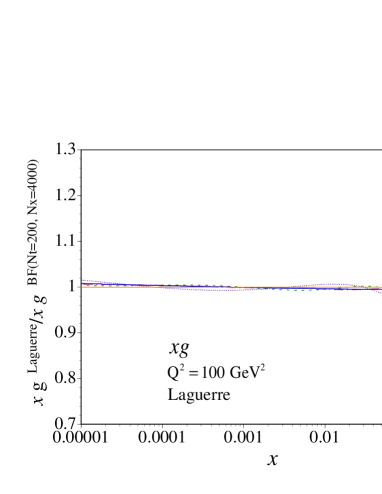
Figure 8: Evolved gluon distribution ratios $xg^{Laguerre}/xg^{BF}$ are shown for $N_{Lag}$=5, 10, 20, and 30 in the Laguerre-polynomial method.

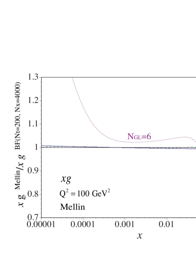
Figure 9: Evolved gluon distribution ratios $xg^{Mellin}/xg^{BF}$ are shown for $N_{GL}$=6, 10, 20, and 50 in the Mellin-transformation method.

4.2 Fragmentation functions

The fragmentation functions (FFs) are essential for understanding hadron productions in high-energy reactions. In addition, they are important for describing ultrahigh-energy cosmic rays in the top-down scenario [4, 5]. In comparison with the situation of the PDFs, their determination is still premature in the sense that experimental data are not still enough to determine them accurately. However, there are available $e^{+}e^{-}$ annihilation data, which could be used for a global analysis of the FFs. The current status of such analyses is summarized in Ref. [2]. We use the KKP parametrization [15] at $Q^{2}$=2 GeV² as the initial functions, and then they are evolved to $Q^{2}$=100 GeV² with the KKP scale parameter for testing three evolution methods.

The brute-force evolution with $N_{t}$=200 and $N_{x}$=4000 is taken as the standard for showing other evolution results as it was done in the previous subsection. In Fig. 11, the Laguerre-method results for the singlet fragmentation function into the proton and antiproton, $D_{q_{s}}^{p+\bar{p}}=\sum_{i}(D_{q_{i}}^{p+\bar{p}}+D_{\bar{q}_{i}}^{p+\bar{p}})$, are shown. The Mellin method results are shown in Fig. 11. The small-$x$ region is shown in these figures for comparing the results with the PDF accuracy in Sec. 4.1, although it is outside the range of current accelerator experiments. As it was found in the PDF evolution, the Laguerre method is not excellent in the small- and large-$x$ regions unless a large number of polynomials is taken. The ratios in Figs. 11 and 11 show a similar tendency to the ratios of the PDF singlet evolution results in Figs. 7 and 7, respectively.

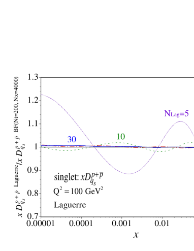
Figure 10: Evolved singlet fragmentation function ratios $xD_{q_{s}}^{p+\bar{p},\ Laguerre}/xD_{q_{s}}^{p+\bar{p},\ BF}$ are shown for $N_{Lag}$=5, 10, 20, and 30 in the Laguerre-polynomial method.

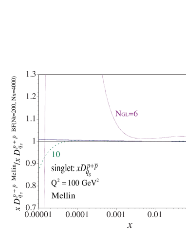
Figure 11: Evolved singlet fragmentation function ratios $xD_{q_{s}}^{p+\bar{p},\ Mellin}/xD_{q_{s}}^{p+\bar{p},\ BF}$ are shown for $N_{GL}$=6, 10, 20, and 50 in the Mellin-transformation method.

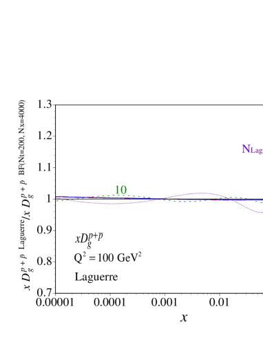
Figure 12: Evolved gluon fragmentation function ratios $xD_{g}^{p+\bar{p},\ Laguerre}/xD_{g}^{p+\bar{p},\ BF}$ are shown for $N_{Lag}$=5, 10, 20, and 30 in the Laguerre-polynomial method.

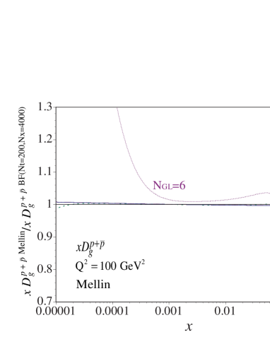
Figure 13: Evolved gluon fragmentation function ratios $xD_{g}^{p+\bar{p},\ Mellin}/xD_{g}^{p+\bar{p},\ BF}$ are shown for $N_{GL}$=6, 10, 20, and 50 in the Mellin-transformation method.

The gluon FF evolution results are shown in Figs. 13 and 13 for the Laguerre and Mellin methods. The gluon FF evolution by the Laguerre method is accurate in the most-$x$ region except for the large-$x$ part. The Mellin method is also accurate except for the large-$x$ region.

We have compared three evolution methods; however, there are other methods [16]. Because the numerical solution of the DGLAP equations is very important for describing high-energy hadron reactions, an efficient and accurate method should be investigated further.

4.3 Computation time

We show typical computation time for each evolution method. However, we should aware that it depends much on the numbers, $N_{t}$ and $N_{x}$ in the brute-force method, $N_{Lag}$ in the Laguerre method, and $N_{GL}$ in the Mellin method. Therefore, we list CPU time for different parameter values for $N_{t}$, $N_{x}$, $N_{Lag}$, and $N_{GL}$ in Table 1 by running the codes for the nonsinglet PDF. In the singlet evolution, the time becomes longer but the tendency of three evolution methods is the same. The used machine is DELL-Dimension-8800 with a Pentiam-4 2.8G CPU. The operating system is Redhat-Linux 8.0 and the fortran complier is g77.

Table 1: CPU time for calculating PDFs at 500 $x$-points by running each evolution code for the nonsinglet distribution with the linux-g77 compiler on a Pentiam-4 machine with a 2.8G CPU.

Method	Condition	CPU time (seconds)
		for PDFs at 500 $x$-points
Brute-force	$N_{t}$=50, $N_{x}$ =1000	1.501
	$N_{t}$=200, $N_{x}$ =1000	5.986
	$N_{t}$=200, $N_{x}$ =4000	95.634
Laguerre	$N_{Lag}$=5	0.005
	$N_{Lag}$=10	0.011
	$N_{Lag}$=20	0.025
	$N_{Lag}$=30	0.044
Mellin	$N_{GL}$=6	0.154
	$N_{GL}$=10	0.244
	$N_{GL}$=20	0.464
	$N_{GL}$=50	1.128

Among the three methods, the brute-force method takes the longest time for the computation simply because the large numbers of steps are taken. Therefore, it typically takes a few seconds for obtaining a reasonable accuracy for the nonsinglet evolution ($N_{t}$=50-200, $N_{x}$=1000).

In the Laguerre method, the evolution is simply given by the summation of the Laguerre coefficients which are calculated partially with the recursion relation. There is no numerical integration involved in the evolution calculation, so that this method is by far the fastest among the studied methods. Even if $N_{Lag}$=30 is taken, it takes 0.044 seconds for the nonsinglet evolution. It means that it is one hundred times faster than the brute-force method. If one is interested in using it for the singlet evolution and if one does not mind one or two percent error, it is certainly the best method.

In the Mellin method, accurate evolution results are obtained with $N_{GL}=20$. The computation time is significantly shorter and it is several times faster than the brute-force method. This is the reason why this method is popular among high-energy physics researchers.

5 Summary

We have compared the evolution results of the parton distribution functions and the fragmentation functions by using three evolution methods, brute-force, Laguerre-polynomial, Mellin-transformation methods. The advantages and disadvantages of each method are summarized in Table 2.

Table 2: Summary of advantages and disadvantages of each evolution method.

Method	Advantage	Disadvantage
Brute-force	Simple code: The computer code is very simple. More complicated evolution equations with higher-twists (e.g. in Ref. [11]) could be handled easily. The evolution could be accurate in the small- and large-$x$ regions.	Long computation time: In order to obtain an accurate evolution, large numbers of steps ($N_{t}$ and $N_{x}$) are needed. If one uses the code for many evolution calculations, it takes a significant amount of time.
Laguerre	Very fast: It takes less than a second by an ordinary desktop computer. As long as one does not mind the very small- and large-$x$ regions, it is a good method for repeated evolution calculations.	Accuracy at small and large $x$: Depending on the initial functional form, the results do not converge at small $x$ unless a large number of polynomials are used. It is also difficult to obtain accurate evolution at large $x$.
Mellin	Fast: By choosing an appropriate $z_{max}$ and $N_{GL}$ in each $x$ region, the code becomes much faster than the brute-force computation. For repeated evolution calculations with certain accuracy, this method is appropriate.	Accuracy at small and large $x$: One should be careful about the choices of $z_{max}$ and $N_{GL}$. In particular, the Mellin inversion should be carefully done at very large $x$.

References

- [1] http://durpdg.dur.ac.uk/hepdata/pdf.html.
- [2] http://www.pv.infn.it/~ radici/FFdatabase/.
- [3] V. N. Gribov and L. N. Lipatov, Sov. J. Nucl. Phys. 15 (1972) 438 and 675; G. Altarelli and G. Parisi, Nucl. Phys. B126 (1977) 298; Yu. L. Dokshitzer, Sov. Phys. JETP 46 (1977) 641.
- [4] R. Toldrà, Comput. Phys. Commun. 143 (2002) 287.
- [5] S. Sarkar and R. Toldrà, Nucl. Phys. B621 (2002) 495. For a general introduction, see F. W. Stecker, J. Phys. G29 (2003) R47.
- [6] N. Cabibbo and R. Petronzio, Nucl. Phys. B137 (1978) 395; G. P. Ramsey, Ph.D. thesis, Illinois Institute of Technology, (1982).
- [7] M. Miyama and S. Kumano, Comput. Phys. Commun. 94 (1996) 185; M. Hirai, S. Kumano, and M. Miyama, Comput. Phys. Commun. 108 (1998) 38; 111 (1998) 150. See http://hs.phys.sasa-u.ac.jp/program.html.
- [8] W. Furmanski and R. Petronzio, Nucl. Phys. B195 (1982) 237; G. P. Ramsey, J. Comput. Phys. 60 (1985) 97; J. Blümlein, G. Ingelman, M. Klein, and R. Rückl, Z. Phys. C45 (1990) 501; S. Kumano and J. T. Londergan, Comput. Phys. Commun. 69 (1992) 373; R. Kobayashi, M. Konuma, and S. Kumano, Comput. Phys. Commun. 86 (1995) 264.
- [9] M. Glück, E. Reya, and A. Vogt, Z. Phys. C48 (1990) 471; D. Graudenz, M. Hampel, A. Vogt, and C. Berger, Z. Phys. C70 (1996) 77; J. Blümlein and A. Vogt, Phys. Rev. D58 (1998) 014020; J. Blümlein, Comput. Phys. Commun. 133 (2000) 76; M. Stratmann and W. Vogelsang, Phys. Rev. D64, 114007 (2001); M. Imoto, personal communications.
- [10] R. K. Ellis, W. J. Stirling, and B. R. Webber, QCD and Collider Physics, Cambridge University Press (1996).
- [11] A. H. Mueller and J. Qiu, Nucl. Phys. B268 (1986) 427.
- [12] M. Glück, E. Reya, M. Stratmann, and W. Vogelsang, Phys. Rev. D63, 094005 (2001); J. Blümlein and H. Böttcher, Nucl. Phys. B636, 225 (2002).
- [13] M. Hirai, S. Kumano, and N. Saito, hep-ph/0312112, Phys. Rev. D in press.
- [14] A. D. Martin, R. G. Roberts, W. J. Stirling, and R. S. Thorne, Phys. Lett. B531 (2002) 216.
- [15] B. A. Kniehl, G. Kramer, and B. Pötter, Nucl. Phys. B582 (2000) 514.
- [16] As an example of recent studies, see S. Jadach and M. Skrzypek, hep-ph/0312355.