Abstract

An analysis of soft breaking under the constraint of modular invariance is given. The role of dilaton and moduli dependent front factors in achieving a modular invariant $V_{soft}$ is emphasized. Further, it is shown that in string models $\tan\beta$ is no longer a free parameter but is determined in terms of $\alpha_{string}$ and the other soft parameters by the constraints of modular invariance and radiative electroweak symmetry breaking. The above framework is then used to analyze the neutralino relic density consistent with the WMAP data at self dual points in the Kähler and complex structure moduli. One finds that the combined set of constraints arising from modular invariant soft breaking, radiative electroweak symmetry breaking and WMAP lead to upper limits on sparticle masses for $\mu>0$. These limits are investigated for a class of models and found to lie within reach of the Tevatron and of the Large Hadron Collider (LHC). Further, an analysis of the neutralino-proton cross section shows that dark matter in these models can be explored in CDMS (Soudan), GENIUS and ZEPLIN. While the analysis is carried out within the general framework of heterotic strings, the possibility that the results of the analysis may extend to a broader class of string models, such as models based on intersecting D branes, is also discussed.

1 Introduction

Recently the Wilkinson Microwave Anisotropy Probe (WMAP)[1, 2] has measured the cosmological parameters to a high degree of accuracy leading to a very precise constraint on the density of cold dark matter (CDM) in the universe. Thus the data suggests an $\Omega_{CDM}h^{2}$ in the range

$$\Omega_{CDM}h^{2}=0.1126^{+0.016}_{-0.018}$$ (1)

Here $\Omega_{CDM}=\rho_{CDM}/\rho_{c}$ where $\rho_{CDM}$ is the mass density of the CDM and $\rho_{c}$ is the critical mass density needed to close the universe, and $h$ is the Hubble parameter in units of 100Km/s.Mpc. The implications of this constraint were analyzed in Ref.[3] in the framework of mSUGRA and quite surprisingly it was found that relic density constraint of Eq. (1) allows for scalar masses to be in the domain of several TeV which may even lie beyond the reach of the LHC (For other analyses of WMAP data see Ref.[4, 5, 6]). This is so because radiative breaking of the electroweak symmetry occurs in part on the so called Hyperbolic Branch/Focus Point region (HB/FP)[7] which contains an inversion region[3] where typically the Higgs mixing parameter $\mu$ is relatively small, i.e., $|\mu|<<m_{0},m_{1/2}$ where $m_{0}$ is the universal scalar mass, $m_{1/2}$ is the universal gaugino mass at the GUT scale $M_{G}\sim 2\times 10^{16}$ GeV, and $\mu$ is the Higgs mixing parameter which appears in the superpotential in the form $\mu H_{1}H_{2}$. In the inversion region the lightest supersymmetric particle (LSP) is the neutralino with mass $\sim|\mu|$ and is degenerate with the next to the lightest neutralino and the light chargino. Consequently there is a lot of coannihilation in this region allowing for the satisfaction of the WMAP relic density constraints even for very large values of $m_{0},m_{1/2}$.

In this paper we show that the situation is drastically different in a class of string models because of the more constrained parameter space[8]. Additionally the constraint of radiative breaking of the electroweak symmetry is more stringent allowing for a determination of $\tan\beta$. Our underlying procedure is to consider effective low energy theory below the string scale for a heterotic string model[9]. We assume this theory to possess a T-duality invariance, specifically an SL(2,Z) modular invariance associated with large-small radius symmetry. Thus we assume that the effective scalar potential in four dimensions depends on the dilaton field $S$ and on the Kähler moduli fields $T_{i}$ (i=1,2,3) and later we will also extend our analysis by including the dependence on the complex structure moduli $U_{i}$. We require the scalar potential of the theory to be invariant under the modular $SL(2,Z)$ T transformations given by

$$T_{i}\rightarrow T^{\prime}_{i}=\frac{{a_{i}T_{i}-ib_{i}}}{{ic_{i}T_{i}+d_{i}}},$$

$$\bar{T}_{i}\rightarrow\bar{T}^{\prime}_{i}=\frac{a_{i}\bar{T}_{i}+ib_{i}}{-ic_{i}\bar{T}_{i}+d_{i}},$$

$$(a_{i}d_{i}-b_{i}c_{i})=1,~{}~{}~{}(a_{i},b_{i},c_{i},d_{i}\in Z).$$ (2)

We follow the approach developed in Ref.[8] (For previous analyses on soft susy breaking in string theory under the constraints of modular invariance see Refs.[10, 11, 12, 13] and for its phenomenology see Refs.[14]). Thus following the supergravity approach adopted in Ref.[15] we assume the superpotential to be composed of a visible sector and a hidden sector so that $W=W_{v}+W_{h}$ where supersymmetry breaks in the hidden sector and is communicated to the visible sector where it leads to generation of soft breaking. The Kähler potential is in general given by

$$d=-ln(S+\bar{S}+\frac{1}{4\pi^{2}}\sum_{i}^{3}\delta_{i}^{GS}log(T_{i}+\bar{T}_{i}))-\sum_{i}log(T_{i}+\bar{T}_{i})+K_{IJ}Q_{I}^{\dagger}Q_{J}+H_{IJ}Q_{I}Q_{J}$$ (3)

where $\delta_{i}^{GS}$ is the one loop Green-Schwarz correction to the Kähler potential[16] and $Q$ are the matter fields consisting of leptons, quarks and the Higgs. For the analysis in this work we assume $\delta_{i}^{GS}=0$. The resulting moduli potential have a form which arises in a class of no scale supergravity [ for a review see [17]]. For the visible sector we assume a general form $W_{v}=\tilde{\mu}_{IJ}Q_{I}Q_{J}+\lambda_{IJK}Q_{I}Q_{J}Q_{K}$. The outline of the rest of the paper is as follows: In Sec.2 we give a pedagogical description of modular properties of various quantities that appear in soft breaking. We emphasize the role of dilaton and moduli dependent front factors in achieving a modular invariant soft breaking and an explicit proof of modular invariance of $V_{soft}$ is also given. In Sec.3 we discuss radiative breaking of the electroweak symmetry in the context of string models and show that $\tan\beta$ is not a free parameter but a determined quantity in string models. In Sec.4 we use the modular invariant soft breaking and the determination of $\tan\beta$ to compute the neutralino relic density in the range allowed by the WMAP data. The cases $\mu>0$ and $\mu<0$ are found to have significantly different behaviors. For the case $\mu>0$ (which appears to be the preferred value of $\mu$[18] from the $g_{\mu}-2$ data[19]) it is shown that the modular invariant soft breaking, the string determined value of $\tan\beta$ and the WMAP constraint combine to produce upper limits on sparticle masses which appear to lie within reach of the hadron colliders for a class of string models. Implications for the direct detection of dark matter are also discussed. Conclusions are given in Sec.5.

2 Modular Invariant Soft Breaking

In this section we give a pedagogic discussion of the modular properties of the soft parameters and also show explicitly that the soft breaking scaler potential is modular invariant. We begin by defining modular weights. Suppose we have a function $f(T_{i},\bar{T}_{i})$ which transforms under modular transformations of Eq. (2) so that

$$f(T_{i},\bar{T}_{i})\rightarrow f(T_{i}^{\prime},\bar{T}_{i}^{\prime})=(icT_{i}+d)^{n_{1}}(-ic\bar{T}_{i}+d)^{n_{2}}f(T_{i},\bar{T}_{i})$$ (4)

then it has modular weight $(n_{1},n_{2})$. For example, from Eq. (2) one finds that $(T_{i}+\bar{T}_{i})$$\rightarrow$$(T_{i}^{\prime}+\bar{T}_{i}^{\prime})$$=(ic_{i}T_{i}+d_{i})^{-1}(-ic_{i}\bar{T}_{i}+d_{i})^{-1}(T_{i}+\bar{T}_{i})$ and thus $(T_{i}+\bar{T}_{i})$ has modular weights $(-1,-1)$. Now $G$ defined by $G=d+ln(WW^{\dagger})$ is invariant under modular transformations which implies that $W$ has modular weight $(-1,0)$ and $W^{\dagger}$ has modular weight $(0,-1)$ under the modular transformation of Eq. (2). Thus $WW^{\dagger}$ has modular weight $(-1,-1)$ and $|W|$ has modular weight (-1/2,-1/2). Defining $\theta_{W}$ so that

$$W=|W|e^{i\theta_{W}}$$ (5)

we find that $e^{i\theta_{W}}$ has modular weight (-1/2, 1/2). The Dedekind function $\eta(T_{i})$ (where $\eta(T_{i})=q^{1/24}\Pi_{n}(1-q^{n})$, $q=e^{2\pi iT_{i}}$) has modular weight (1/2,0) while $G_{2}(T_{i})$ defined by

$$G_{2}(T_{i})=\frac{\partial ln\eta^{2}(T_{i})}{\partial T_{i}}+\frac{1}{T_{i}+\bar{T}_{i}}$$ (6)

has modular weight (2,0). More generally if we have a function $Q(T_{i})$ with modular weight $(n_{Q}^{i},0)$ then the covariant derivative defined by

$$D_{T_{i}}[lnQ(T_{i})]\equiv\frac{\partial lnQ(T_{i})}{\partial T_{i}}+\frac{n_{Q}^{i}}{T_{i}+\bar{T}_{i}}$$ (7)

transforms as

$$D_{T_{i}}[lnQ(T_{i})]\rightarrow D_{T_{i}^{\prime}}[lnQ(T_{i}^{\prime})]=(icT_{i}+d)^{2}D_{T_{i}}[lnQ(T_{i})]$$ (8)

and thus $D_{T_{i}}[lnQ(T_{i})]$ has modular weight $(2,0)$.

In Table 1 we summarize modular weights of several quantities that appear in the analysis of soft breaking. We consider now the specific model of Ref.[8]. For $W_{h}$ we assume that the modular weight is carried by the Dedekind function $\eta(T_{i})$ so that $W_{h}={F(S,T_{i})}/{\prod_{i=1}^{3}\eta(T_{i})^{2}}$, where $F(S,T_{i})$ is modular invariant. For the Kähler potential we consider the specific form $d=D(S,\bar{S})$ -$\sum_{i}ln(T_{i}+\bar{T}_{i})$+$\sum_{i\alpha}(T_{i}+\bar{T}_{i})^{n_{\alpha}^{i}}$ $C_{\alpha}^{\dagger}C_{\alpha}$, where $C_{\alpha}$ are the charged fields with modular weights $n^{i}_{\alpha}$. We introduce the notation $\gamma_{s}=(S+\bar{S})G,S/\sqrt{3}$ $=|\gamma_{S}|e^{i\theta_{S}}$, $\gamma_{T_{i}}=(T_{i}+\bar{T}_{i})G,{T_{i}}/\sqrt{3}$ $=|\gamma_{T_{i}}|e^{i\theta_{T_{i}}}$. The condition that vacuum energy vanish then takes the form

$$|\gamma_{S}|^{2}+\sum_{i=1}^{3}|\gamma_{T_{i}}|^{2}=1$$ (9)

quantity	modular weights
$|W|$	$(-\frac{1}{2},-\frac{1}{2})$
$e^{i\theta_{W}}$	$(-\frac{1}{2},\frac{1}{2})$
$\eta(T_{i})$	$(\frac{1}{2},0)$
$2\partial_{T_{i}}ln\eta(T_{i})+(T_{i}+\bar{T}_{i})^{-1}$	$(2,0)$
$\partial_{T_{i}}W-(T_{i}+\bar{T}_{i})^{-1}W$	$(1,0)$
$Y_{\alpha\beta\gamma}(T_{i})$	$(-1-n_{\alpha\beta\gamma}^{i},0)$
$\lambda_{\alpha\beta\gamma}(T_{i})$	$(0,0)$
$\partial_{T_{i}}lnY_{\alpha\beta\gamma}(T_{i})-(1+n_{\alpha\beta\gamma}^{i})(T_{i}+\bar{T}_{i})^{-1}$	$(2,0)$
$\mu_{\alpha\beta}(T_{i})$	$(-1-n_{\alpha\beta}^{i},0)$
$\tilde{\mu}_{\alpha\beta}(T_{i})$	$(0,0)$
$\partial_{T_{i}}ln\mu_{\alpha\beta}(T_{i})-(1+n_{\alpha\beta}^{i})(T_{i}+\bar{T}_{i})^{-1}$	$(2,0)$
$\partial_{T_{i}}\lambda_{\alpha\beta\gamma}(T_{i})$	$(2,0)$
$\partial_{T_{i}}\tilde{\mu}_{\alpha\beta}(T_{i})$	$(2,0)$
$(T_{i}+\bar{T}_{i})$	$(-1,-1)$
$|\gamma_{s}|$	$(0,0)$
$|\gamma_{T_{i}}|$	$(0,0)$
$e^{i\theta_{T_{i}}}$	$(1,-1)$
$e^{i\theta_{S}}$	$(0,0)$
$A^{0}_{\alpha\beta\gamma}$	$(1,0)$
$B^{0}_{\alpha\beta}$	$(1,0)$
$1/\sqrt{f}$	($\frac{1}{2}$,$\frac{1}{2}$)

Table 1: A list of modular weights under the modular transformations of Eq. (2)

The soft breaking potential for this case is given by

$$V_{soft}=m_{3/2}^{2}\sum_{\alpha}(1+3\sum_{i=1}^{3}n^{i}_{\alpha}|\gamma_{T_{i}}|^{2})c_{\alpha}^{\dagger}c_{\alpha}+(\sum_{\alpha\beta}B^{0}_{\alpha\beta}w^{(2)}_{\alpha\beta}+\sum_{\alpha\beta\gamma}A_{\alpha\beta\gamma}^{0}w_{\alpha\beta\gamma}^{(3)}+H.c.)$$ (10)

where the normalized fields $c_{\alpha}$ and $m_{3/2}$ ($=e^{-G/2}$) are modular invariant and $w^{(2)}_{\alpha\beta}=\mu_{\alpha\beta}C_{\alpha}C_{\beta}$ and $w^{(3)}_{\alpha\beta\gamma}=Y_{\alpha\beta\gamma}C_{\alpha}C_{\beta}C_{\gamma}$. Following the standard procedure the soft breaking parameters $A^{0}$ and $B^{0}$ may be expressed in the form

$$A_{\alpha\beta\gamma}^{0}=-\sqrt{3}m_{3/2}\frac{e^{D/2-i\theta_{W}}}{\sqrt{f}}[|\gamma_{S}|e^{-i\theta_{S}}(1-(S+\bar{S})\partial_{S}lnY_{\alpha\beta\gamma})$$

$$+\sum_{i=1}^{3}|\gamma_{T_{i}}|e^{-i\theta_{T_{i}}}(1+n^{i}_{\alpha}+n^{i}_{\beta}+n^{i}_{\gamma}-(T_{i}+\bar{T}_{i})\partial_{T_{i}}lnY_{\alpha\beta\gamma}-(T_{i}+\bar{T}_{i})n^{i}_{\alpha\beta\gamma}G_{2}(T_{i}))]$$ (11)

and

$$B_{\alpha\beta}^{0}=-m_{3/2}\frac{e^{D/2-i\theta_{W}}}{\sqrt{f}}[1+\sqrt{3}|\gamma_{S}|e^{-i\theta_{S}}(1-(S+\bar{S})\partial_{S}ln\mu_{\alpha\beta})$$

$$+\sqrt{3}\sum_{i=1}^{3}|\gamma_{T_{i}}|e^{-i\theta_{T_{i}}}(1+n^{i}_{\alpha}+n^{i}_{\beta}-(T_{i}+\bar{T}_{i})\partial_{T_{i}}ln\mu_{\alpha\beta}-(T_{i}+\bar{T}_{i})n^{i}_{\alpha\beta}G_{2}(T_{i}))]$$ (12)

The modular properties of $A_{\alpha\beta\gamma}^{0}$ and $B_{\alpha\beta}^{0}$ are not so manifest as written in the above form. This is so because $\partial_{T_{i}}(lnY_{\alpha\beta\gamma})$ and $\partial_{T_{i}}(ln\mu_{\alpha\beta})$ have no well defined modular weights. Indeed they are mixtures of terms with different modular weights. Thus we may express them as follows

$$\partial_{T_{i}}(lnY_{\alpha\beta\gamma})=D_{T_{i}}(lnY_{\alpha\beta\gamma})+(1+n^{i}_{\alpha\beta\gamma})(T_{i}+\bar{T}_{i})^{-1}$$

$$\partial_{T_{i}}(ln\mu_{\alpha\beta})=D_{T_{i}}(ln\mu_{\alpha\beta})+(1+n^{i}_{\alpha\beta})(T_{i}+\bar{T}_{i})^{-1}$$

$$n^{i}_{\alpha\beta\gamma}=n^{i}_{\alpha}+n^{i}_{\beta}+n^{i}_{\gamma},~{}~{}n^{i}_{\alpha\beta}=n^{i}_{\alpha}+n^{i}_{\beta}$$ (13)

where $D_{T_{i}}(lnY_{\alpha\beta\gamma})$ and $D_{T_{i}}(ln\mu_{\alpha\beta})$ have modular weight $(2,0)$ while $(T_{i}+\bar{T}_{i})^{-1}$ has modular weight ($1,1)$. Thus we see that $\partial_{T_{i}}(lnY_{\alpha\beta\gamma})$ and $\partial_{T_{i}}(ln\mu_{\alpha\beta})$ are a linear combination of quantities with modular weight (2,0) and (1,1). Using Eq. (13) we may express Eqs. (11) and (12) in the form

$$A_{\alpha\beta\gamma}^{0}=m_{3/2}\frac{e^{D/2-i\theta_{W}}}{\sqrt{f}}\sqrt{3}\sum_{i=1}^{3}|\gamma_{T_{i}}|(T_{i}+\bar{T}_{i})e^{-i\theta_{T_{i}}}[n^{i}_{\alpha\beta\gamma}G_{2}(T_{i})+D_{T_{i}}lnY_{\alpha\beta\gamma}]$$

$$-m_{3/2}\frac{e^{D/2-i\theta_{W}}}{\sqrt{f}}\sqrt{3}|\gamma_{S}|e^{-i\theta_{S}}(1-(S+\bar{S})\partial_{S}lnY_{\alpha\beta\gamma})$$ (14)

and

$$B_{\alpha\beta}^{0}=m_{3/2}\frac{e^{D/2-i\theta_{W}}}{\sqrt{f}}\{-1+\sqrt{3}\sum_{i=1}^{3}|\gamma_{T_{i}}|(T_{i}+\bar{T}_{i})e^{-i\theta_{T_{i}}}[n^{i}_{\alpha\beta}G_{2}(T_{i})+D_{T_{i}}ln\mu_{\alpha\beta}]\}$$

$$-m_{3/2}\frac{e^{D/2-i\theta_{W}}}{\sqrt{f}}\sqrt{3}|\gamma_{S}|e^{-i\theta_{S}}(1-(S+\bar{S})\partial_{S}ln\mu_{\alpha\beta})$$ (15)

The modular properties of $A^{0}$ and $B^{0}$ can be easily read off from above. Using Table 1, we find that in Eq. (14) the front factor $e^{D/2-i\theta_{W}}/\sqrt{f}$ has a modular (1,0) and the remaining factors have modular weight (0,0) giving $A^{0}$ an overall modular weight (1,0) as desired. The same also holds for $B^{0}$ as can be read off from Eq.(15). While expressions of Eqs.(14) and (15) are useful in exhibiting the modular properties of $A^{0}$ and $B^{0}$, they (as well as Eqs. (11) and (12)) seem to imply at least superficially that $A^{0}$ and $B^{0}$ have a significant dependence on the modular weights. This is not really the case as we now demonstrate. To this end we define modular invariant couplings $\lambda_{\alpha\beta\gamma}$ and $\tilde{\mu}_{\alpha\beta}$ so that

$$Y_{\alpha\beta\gamma}=\lambda_{\alpha\beta\gamma}\eta^{-2(1+n^{i}_{\alpha\beta\gamma})}(T_{i}),~{}~{}=\mu_{\alpha\beta}=\tilde{\mu}_{\alpha\beta}\eta^{-2(1+n^{i}_{\alpha\beta})}(T_{i})$$ (16)

where $\lambda_{\alpha\beta\gamma}$ and $\tilde{\mu}_{\alpha\beta}$ have modular weights $(0,0)$. We note the following identity

$$\partial_{T_{i}}lnY_{\alpha\beta\gamma}=\partial_{T_{i}}ln\lambda_{\alpha\beta\gamma}-(1+n^{i}_{\alpha}+n^{i}_{\beta}+n^{i}_{\gamma})G_{2}(T_{i})+\frac{1+n^{i}_{\alpha}+n^{i}_{\beta}+n^{i}_{\gamma}}{T_{i}+\bar{T}_{i}}$$ (17)

which can be gotten by using the relation $\partial_{T_{i}}ln\lambda_{\alpha\beta\gamma}=D_{T_{i}}(lnY_{\alpha\beta\gamma})+(1+n^{i}_{\alpha\beta\gamma})G_{2}(T_{i})$ and Eq. (13). Using Eq. (17) in Eq. (11) we may write $A_{\alpha\beta\gamma}^{0}$ as follows

$$A_{\alpha\beta\gamma}^{0}=m_{3/2}\frac{e^{D/2-i\theta_{W}}}{\sqrt{f}}\sqrt{3}\sum_{i=1}^{3}|\gamma_{T_{i}}|(T_{i}+\bar{T}_{i})e^{-i\theta_{T_{i}}}[-G_{2}(T_{i})+\partial_{T_{i}}ln\lambda_{\alpha\beta\gamma}]$$

$$-m_{3/2}\frac{e^{D/2-i\theta_{W}}}{\sqrt{f}}\sqrt{3}|\gamma_{S}|e^{-i\theta_{S}}(1-(S+\bar{S})\partial_{S}lnY_{\alpha\beta\gamma})$$ (18)

and a similar analysis gives

$$B_{\alpha\beta}^{0}=m_{3/2}\frac{e^{D/2-i\theta_{W}}}{\sqrt{f}}\{-1+\sqrt{3}\sum_{i=1}^{3}|\gamma_{T_{i}}|(T_{i}+\bar{T}_{i})e^{-i\theta_{T_{i}}}[-G_{2}(T_{i})+\partial_{T_{i}}ln\tilde{\mu}_{\alpha\beta}]\}$$

$$-m_{3/2}\frac{e^{D/2-i\theta_{W}}}{\sqrt{f}}\sqrt{3}|\gamma_{S}|e^{-i\theta_{S}}(1-(S+\bar{S})\partial_{S}ln\mu_{\alpha\beta})$$ (19)

In Eqs. (18) and  (19) one finds that the modular weights have disappeared due to the cancellation arising out of the identity Eq. (17). Further, using Table 1 we find that the modular weight of $A^{0}$ is manifestly (1,0) and similarly the modular weight of $B^{0}$ is (1,0) as necessary to achieve a modular invariant $V_{soft}$. The importance of the front factors $e^{D/2-i\theta_{W}}/\sqrt{f}$ was first emphasized in the work of Ref.[8]. This factor is often suppressed or omitted in string based analyses of soft breaking. However, since it has a non vanishing modular weight, the modular invariance of $V_{soft}$ cannot be maintained without it. Further, the front factor $e^{D/2}$ is also significant in another context as will be discussed in Sec.3.

The analysis given above is more general than of Ref. ([8]). We can limit to that result by making a further dynamical assumption. Thus while $\lambda_{\alpha\beta\gamma}$ and $\tilde{\mu}_{\alpha\beta}$ have modular weights $(0,0)$ they could still have modular dependence through dependence on modular invariants. A significant simplification occurs if we assume that this dependence is identical to that of the function $F(S,T_{i})$. Specifically we assume that $\partial_{T_{i}}\lambda_{\alpha\beta\gamma}=\partial_{T_{i}}F(S,T_{i})$ and $\partial_{T_{i}}\tilde{\mu}_{\alpha\beta}=\partial_{T_{i}}F(S,T_{i})$. Under this assumption and also assuming that the potential is minimized at the self dual points $T_{i}=(1,e^{i\pi/6})$ one finds[8]

$$A_{\alpha\beta\gamma}^{0}=m_{3/2}e^{D/2-i\theta_{W}}(3\sum_{i=1}^{3}|\gamma_{T_{i}}|^{2}-\sqrt{3}|\gamma_{S}|(1-(S+\bar{S})\partial_{S}lnY_{\alpha\beta\gamma})e^{-i\theta_{s}})/f_{\alpha}^{\frac{1}{2}}$$ (20)

$$B^{0}_{\alpha\beta}=m_{3/2}e^{D/2-i\theta_{W}}(-1+3\sum_{i=1}^{3}|\gamma_{T_{i}}|^{2}-\sqrt{3}|\gamma_{S}|(1-(S+\bar{S})\partial_{S}ln\mu)e^{-i\theta_{s}})/f_{\alpha}^{\frac{1}{2}}$$ (21)

where $f_{\alpha}$ arises due to the possibility of several degenerate vacua so that $\{f_{\alpha}\}=8,4\sqrt{3}$, $6$, $3\sqrt{3}$. We can easily extend the above analysis to include the complex structure moduli $U_{i}$ (i=1,2,3) which have $SL(2,Z)$ modular transformations of their own under which the scalar potential is invariant. Including the $U_{i}$ moduli the Kähler potential is of the form

$$d=-ln(S+\bar{S})-\sum_{i=1}^{3}log(T_{i}+\bar{T}_{i})-\sum_{i=1}^{3}log(U_{i}+\bar{U}_{i})$$ (22)

It is convenient to relabel the $U_{i}$ moduli so that $T_{3+i}=U_{i}$ (i=1,2,3). Then assuming that the potential is minimized again at the self dual points for all $T_{i}$, Eqs. (20) and  (21) are valid with i summed from $1-6$ where $f_{\alpha}$ assume the set of values $2^{n}3^{3-\frac{n}{2}}$ (n=0,..,6). Further, in Eq. (9) the sum over i runs from $1-6$. Gauginos also acquire masses after spontaneous breaking of supersymmetry so that $M_{\alpha}=\frac{1}{2}{Ref_{\alpha}}^{-1}e^{-G/2}f_{\alpha a}(G^{-1})^{a}_{b}G^{b}$, where $f_{\alpha}$ is the gauge kinetic energy function for the case of a product gauge group $\cal G=\prod\cal G_{\alpha}$ and has the expansion $f_{\alpha}=k_{\alpha}S+\sum\frac{1}{4\pi^{2}}[C({\cal G}_{\alpha})-\sum_{I}T(R^{\alpha}_{Q_{I}})(1+2n^{i}_{Q_{I}})-2k_{\alpha}\delta^{GS}_{i}]log(\eta(T_{i}))+\dots,$ where $k_{\alpha}$ is the Kac-Moody level for ${\cal G}_{\alpha}$. In our analysis we limit ourselves to Kac-Moody level 1 and to the universal case so that

$$m_{1/2}=\sqrt{3}m_{3/2}|\gamma_{S}|e^{-i\theta_{s}}$$ (23)

3 Determination of $\tan\beta$ from Modular Invariance and EWSB Constraints

Radiative electroweak symmetry breaking (EWSB) constraints are more stringent in string theory than in supergravity. Radiative symmetry breaking produces two constraints arising from the minimization with respect to the vacuum expectation values of the two Higgs fields $v_{1}=<H_{1}^{0}>$ and $v_{2}=<H_{2}^{0}>$ of the minimal supersymmetric standard model (MSSM), i.e., $\partial V/\partial v_{i}^{0}=0$. Typically in supergravity one of these is used to determine $\mu$ and the other one to eliminate the parameter $B_{0}$ in terms of $\tan\beta$. Now in string theory one has in principle a determination of the parameter $\mu$ and the fact that it should equal the $\mu$ determined via radiative breaking of the electroweak symmetry would be highly constraining. In practice there is no realistic string determination of $\mu$ (see, however, Ref.[20]), and thus pending such a determination we will continue to use the radiative symmetry breaking equation for the computation of the $\mu$ parameter. The second symmetry breaking constraint which eliminates $B_{0}$ in favor of $\tan\beta$ (see, e.g., Ref.[21]) as a parameter in supergravity must be treated differently in string theory since one has a determination of $B_{0}$ here. A remarkable aspect of the $B_{0}$ determination is that it has a front factor of $e^{D/2}$ which is related to the string constant via the relation $e^{-D}=\frac{2}{g_{string}^{2}}$ where $g_{string}=k_{i}g_{i}$ and $k_{i}$ is the Kac-Moody level of the gauge group ${\cal G}_{i}$ and $g_{i}$ is the corresponding gauge coupling constant. Thus the second radiative symmetry breaking equation can be thought of as a determination of the string constant in the terms of parameters at the electroweak scale. Alternately we can think of this second equation as a determination of $\tan\beta$ so that

$$\tan\beta=\frac{(\mu^{2}+\frac{1}{2}M_{Z}^{2}+m_{H_{1}}^{2})f_{\alpha}^{1/2}}{\sqrt{2\pi}\mu m_{3/2}\tilde{r}_{B}\alpha_{string}}(|-1+3\sum_{i}|\gamma_{i}|^{2}-\sqrt{3}|\gamma_{S}|(1-(S+\bar{S})\partial_{S}ln\mu)|)^{-1}$$ (24)

where $\tilde{r}_{B}=r_{B}(1+\epsilon_{Z})$ is the renormalization group coefficient that relates $B$ at the electroweak scale to $B_{0}$ at the unification scale so that $B=r_{B}B_{0}$ and $\epsilon_{Z}=M_{Z}^{2}/(m_{H_{1}}^{2}+\mu^{2}-\frac{1}{2}M_{Z}^{2}+(m_{H_{1}}^{2}+\mu^{2}+\frac{1}{2}M_{Z}^{2})\cot^{2}\beta)$. In this analysis we adopt the procedure of using Eq. (24) to determine $\tan\beta$.

However, care should be taken in implementing Eq.(24). Since Eq.(24) arises from minimization of $V_{Higgs}$ at a higher scale $Q$, i.e., $Q\sim m_{\tilde{t}}$ or $Q\sim$ (highest mass of the spectrum)/2 [7], where the correction to $\mu^{2}$ from the one loop correction of the effective potential is small, one has to consider the value of $m_{H_{1}}^{2}$, $m_{H_{2}}^{2}$, and $\mu^{2}$ at this scale $Q$ while using Eq.(24). This is important since $m_{H_{1}}^{2}$ and $m_{H_{2}}^{2}$ can vary a lot between $Q\sim M_{Z}$ and $Q\sim m_{\tilde{t}}$ etc. In this analysis considering one loop correction to the effective potential we have adopted an iterative procedure to determine $\tan\beta$. This is done by starting with a guess value of $\tan\beta$ then using it to compute $B_{0}$ (via $B(Q)$) from the radiative electroweak symmetry breaking equation and then comparing with the string determined value of $B_{0}$. Such iterations produce rapid convergence of the $B_{0}$ value as obtained from the radiative electroweak symmetry breaking toward its string value. Thus $\tan\beta$ is determined for given values of the soft parameters, input moduli etc., i.e., the choice of the self dual point and $\alpha_{string}$.

4 Analysis of Dark Matter and Sparticle Masses at Self Dual Points with WMAP Constraints

We discuss now the numerical results of the analysis. For simplicity we will set $n_{\alpha}^{i}=0$, assume no dependence on the moduli $U_{i}$ (the dependence on the $U_{i}$ moduli will be considered later) and further assume that one is at the self dual point given by $f_{\alpha}=8$. In the analysis we set all the CP phases to zero. In Fig. 1(a), for $\mu>0$, we give a plot of the self consistent determination of $\tan\beta$ and exhibit it as contours in the $\gamma_{s}-m_{3/2}$ plane for values of $m_{3/2}$ ranging up to 2 TeV. One finds a steady decrease of $\tan\beta$ as $\gamma_{s}$ is increased for a given $m_{3/2}$. Contours of $A_{0}$ and $\mu$ are also shown. Regarding $\mu$, for a given $m_{3/2}$ (i.e., for a given value of the universal scalar mass at $M_{G}$) $\mu$ increases with increasing $\gamma_{s}$ because the universal gaugino mass at $M_{G}$ increases with increasing $\gamma_{S}$. Further, $\mu$ also increases with increasing $m_{3/2}$ for fixed $\gamma_{s}$ since both the universal scalar mass and the universal gaugino mass at $M_{G}$ increase with increasing $m_{3/2}$. In the analysis we also impose the flavor changing neutral current (FCNC) constraint from the process $b\rightarrow s+\gamma$[22, 23, 24, 25] for which we take the range $2\times 10^{-4}<Br(b\rightarrow s+\gamma)<4.5\times 10^{-4}$. In Fig. 1(a) the FCNC constraint is shown as a dot-dashed line below which the region is disallowed. Remarkably one finds that the WMAP relic density limits ($0.094<\Omega_{\tilde{\chi}_{1}^{0}}h^{2}<0.129$) are satisfied within this very constrained system and most of the allowed parameter space is in the dilaton dominated region with $\gamma_{s}>0.6$. The gray region-I in Fig. 1(a) refers to the the non-perturbative zone where the third generation of Yukawa couplings no longer stay within the perturbative limits because of very large $\tan\beta$ values. The gray region II results from the absence of radiative electroweak symmetry breaking (REWSB) condition or smaller $m_{\tilde{\chi}_{1}^{\pm}}$ below the experimental lower limit. In Fig. 1(b) we exhibit the satisfaction of the WMAP relic density constraints in the $\gamma_{s}-\tan\beta$ plane for $\mu>0$. The contours of $m_{3/2}$ are exhibited and so is the FCNC constraint from $b\rightarrow s+\gamma$ (the disallowed region is in the left of the dashed line). From Figs. 1(a) and 1(b) one finds that $m_{3/2}$ consistent with WMAP constraint increases with increasing $\tan\beta$. However, even with $\tan\beta$ as large as $60$ one finds that $m_{3/2}$ is no larger than 500 GeV in order that one satisfy simultaneously the WMAP constraints and the requirement of $\tan\beta$ becoming not too large so that all the Yukawa couplings stay within the perturbative domain.

A plot of the mass spectrum as a function of $\gamma_{s}$ with determined $\tan\beta$ but without the imposition of the relic density constraint is given in Fig. 2(a). A similar analysis as a function of $m_{3/2}$ is given in Fig. 2(b) but again without the imposition of the relic density constraints. Inclusion of the relic density constraint limits $m_{3/2}$ to lie lower than about 500 GeV and the corresponding upper limits on sparticle masses can be read off from Fig. 2(b). In this case the upper limits on sparticle masses all lie roughly below 2 TeV and all are essentially accessible at the LHC. We note that the gluino is the highest mass particle over most of the allowed parameter space of the model. Inclusion of the FCNC constraint drastically lowers the upper limits so that the gluino mass lies below $500$ GeV and masses of the other particles are even lower. Thus some of the particles may also be accessible at the Tevatron. Another interesting phenomenon is that over most of the allowed parameter space the neutralino is the lowest mass supersymmetric particle (LSP) and thus with R parity a candidate for cold dark matter.

In Fig. 3(a) we give a plot of the neutralino-proton scalar cross section $\sigma_{\chi p}$ as a function of the neutralino mass for $\mu>0$. The region with black circles satisfies the WMAP constraint. Also exhibited are the sensitivities that will be reached by experiment, i.e., CDMS (Soudan)[26], GENIUS[27] and ZEPLIN[28, 29] (shown as two broad bands). In Fig. 3(a) we have included the limit from the first set of data from CDMS(Soudan) as announced recently[30] as well as the latest contour from EDELWEISS[31]. The dotted enclosed region is the contour from DAMA[32]. The analysis shows that in this class of string models dark matter falls within the sensitivity that will be achievable at the CDMS (Soudan), GENIUS and ZEPLIN. A similar analysis for the spin dependent neutralino-proton cross section $\sigma_{\chi p}$ as a function of the neutralino mass is given in Fig. 3(b) for $\mu>0$. The region with black circles satisfies the WMAP constraint.

The $\mu<0$ case is analyzed in Figs. (4)-(6). In Fig. (4) contours of $\tan\beta$, and $\mu$ are shown in the $\gamma_{s}-m_{3/2}$ plane. The constraint from $b\rightarrow s+\gamma$ is shown as a dot-dashed line below which the region is disallowed. The WMAP satisfied relic density region is shown as a small shaded area in black. The disallowed gray region I and III is discarded typically due to the absence of a $\tan\beta$ solution consistent with GUT scale inputs. The region II typically refers to the absence of REWSB, or having smaller than experimental lower limits of $m_{\tilde{\chi}_{1}^{\pm}}$. The region IV is a no solution zone like I and III, but its location and extent depends on the sensitivity of the minimization scale for REWSB. The region V is excluded because of tachyonic $\tilde{\tau}_{1}$. An important point to note for $\mu<0$ case is that a given $\tan\beta$ contour has two separate regions, corresponding to smaller and larger $\gamma_{s}$ values for a given $m_{3/2}$. Furthermore, $\tan\beta$ is severely constrained to lie below 20 for $\mu<0$. Unlike the $\mu>0$ case, the $\mu<0$ branch has a larger region where $|\mu|$ is very small, close to its value constrained by the lighter chargino mass lower limit. Further, $m_{3/2}$ here can acquire values much larger than in the $\mu>0$ case consistent with the WMAP constraint and the REWSB appears to be occurring on the hyperbolic branch. Fig. 4(b) shows contours of $m_{3/2}$ in $\gamma_{s}-\tan\beta$ plane for $\mu<0$. The lightly shaded areas (in cyan) satisfy the $b\rightarrow s+\gamma$ limits. In contrast, areas marked with black dots do not satisfy the $b\rightarrow s+\gamma$ bounds. The WMAP allowed region is shown in small filled circles in black. Clearly, the WMAP constraint along with $b\rightarrow s+\gamma$ restricts $\tan\beta$ to be within $12$ to $15$ . A plot of the mass spectrum as a function of $\gamma_{s}$ is given in Fig. 5(a). A similar analysis as a function of $m_{3/2}$ is given in Fig. 5(b). Fig. 6(a) shows a plot of the neutralino-proton scalar cross section $\sigma_{\chi p}$ vs neutralino mass for $\mu<0$. Here the detection cross sections are smaller than the case for $\mu>0$. However, the values of spin-dependent cross section of Fig. 6(b) for $\mu<0$ are much higher than the case when $\mu>0$.

We discuss now the dependence of the analysis on the choice of the self dual point. In Figs. (7) and (8) we give the analysis for the case when $f_{\alpha}=3\sqrt{3}$. A comparison of Fig. (7) with Fig. (1(a)) and with Fig. (3(a)) for the $\mu>0$ case shows that the analysis at the self dual point $f_{\alpha}=3\sqrt{3}$ follows a similar pattern as the analysis at the self dual point $f_{\alpha}=8$. The main difference is the lowering of the maximum in $m_{\frac{3}{2}}$ by about a 100 GeV without imposition of the $b\rightarrow s+\gamma$ constraint. However, when $b\rightarrow s+\gamma$ constraint is imposed there is no significant change with respect to the result corresponding to $f_{\alpha}=8$. For the $\mu<0$ case a comparison of Figs. (8) with Fig. (4(a)) and with Fig. (6(a)) shows that the spin independent $\sigma_{\chi p}$ cross section can dip lower for the case $f_{\alpha}=3\sqrt{3}$ compared to the case when $f_{\alpha}=8$. Aside from that the features of Figs. (8) are very similar to those of Fig. (4(a)) and with Fig. (6(a)).

We now analyze the effect of including the complex structure moduli $U_{i}$. In Fig.(9(a)) we present a composite analysis for relic density and $Br(b\rightarrow s+\gamma)$ in $(\gamma_{s}-m_{3/2})$ plane for $\mu>0$. Here we include $U_{i}$ moduli and we scan over the self dual points corresponding to all possible values of $f_{\alpha}:2^{n}3^{3-n/2},n=0,...6$. This generates maximally allowed regions since we are integrating over all allowed values of $f_{\alpha}$. The $b\rightarrow s+\gamma$ contour is shown as a dot-dashed line below which the region is maximally disallowed. The discarded region by $b\rightarrow s+\gamma$ constraint extends up to $m_{3/2}=750$ GeV. The WMAP satisfied relic density region is maximally shown as small shaded area in black and the region is not much different from the result of Fig.(1(a)) and Fig.(7(a)). Similarly, Fig.(9(b)) does not show much different spin independent LSP-proton cross sections in comparison to Fig.(3(a)) and Fig.(7(b)). We do a similar analysis for relic density for $\mu<0$ in Fig.(10(a)). The result shows that the WMAP allowed region lies in the range $\gamma_{s}=0.1-0.2$ which is more constraining towards smaller $\gamma_{s}$ values in comparison with the similar cases of Fig.(4(a)) and Fig.(8(a)). The spin independent detection cross section result is shown in Fig.(10(b)). In this case most of the points consistent with WMAP constraint lie at values of ${\tilde{m}}_{\chi^{0}_{1}}>>500$ GeV and fall outside the displayed range. Thus the number of point consistent with the WMAP constraint lying below ${\tilde{m}}_{\chi^{0}_{1}}=500$ GeV is very sparce as is evident from Fig.(10(b)) where a few scattered points shown in black circles satisfies the WMAP constraint. However, the range of detection cross sections for WMAP satisfying points is not different from those of Fig.(6(a)) and Fig.(8(b)). Thus we conclude that the inclusion of the complex structure moduli $U_{i}$ does not cause any significant alteration in sparticle mass limits or detection cross section than the results without them. Another interesting observation is that the case $\mu>0$ shows that the region consistent with the WMAP constraint is the dilaton dominated region where $|\gamma_{s}|>0.5$ while the case $\mu<0$ shows that the region consistent with the WMAP constraint is the moduli dominated region where $|\gamma_{s}|<0.5$. Inclusion of $U_{i}$ moduli for $\mu<0$ further restricts $\gamma_{s}$ so that $|\gamma_{s}|<0.2$. It should be interesting to see if this phenomenon is a generic feature in a wider class of string based models.

The analysis above shows that dark matter that results in string models with determined $\tan\beta$ is much more stringently constrained than in models where $\tan\beta$ is taken as a free parameter (For a sample of recent analyses see Refs.[33, 34, 35, 36, 37] and for a recent review see Ref.[38] ). While the above analysis is carried out in the framework of heterotic string models, similar considerations may apply to other classes of string models. Thus recently there has been a great deal of activity in the intersecting brane models (see, e.g, Ref.[39, 40] and the references therein) and specifically semi realistic models with 3 generations and N=1 supersymmetry have been constructed[41]. The pattern of supersymmetry breaking in a broad class of such intersecting D brane models has been analyzed in Ref. ([42, 43]) and some common features with the soft breaking in heterotic string models are shown to emerge. Further, one expects that the constraint of radiative breaking of the electroweak symmetry in the intersecting D brane models would be very similar to the one in the heterotic string models allowing once again a determination of $\tan\beta$. Thus we also expect upper limits on sparticle masses to emerge from the WMAP relic density constraint for the intersecting D brane models at least for the $\mu$ positive case.

5 Conclusion

In conclusion, in this paper we have analyzed the implications of modular invariant soft breaking in a generic heterotic string scenario under the constraint of radiative breaking of the electroweak symmetry. We have emphasized the importance of dilaton and moduli dependent front factors which are shown to be essential in achieving a modular invariant $V_{soft}$. Several forms of the soft parameters $A^{0}$ and $B^{0}$ are exhibited, including the forms which exhibit explicitly their modular weights. It is shown that in models of this type $\tan\beta$ is no longer an arbitrary parameter but a determined quantity. The constraints of modular invariance along with a determined $\tan\beta$ define the allowed parameter space very sharply. Quite interestingly one finds that this parameter space allows for the satisfaction of the accurate relic density constraints given by WMAP. Further, the WMAP constraint combined with the FCNC constraint puts upper limits on the sparticle masses for the case $\mu>0$ which are remarkably low for a class of models implying that essentially all of the sparticles would be accessible at the LHC. Quite remarkably some of the sparticle spectrum should also be accessible at the Tevatron. Further, an analysis of the neutralino proton cross section indicates that this cross section should be accessible at the future dark matter experiments. The analysis presented here reveals that for the class of models considered the region of the parameter space consistent with the WMAP constraints is dilaton dominated for $\mu>0$ and moduli dominated for $\mu<0$. It should be interesting to see if this result holds for a broader class of string based models where $\tan\beta$ is again fixed by the constraints of duality and the radiative breaking of the electroweak symmetry. Finally, we emphasize that the analysis presented here is the first work where the constraint of a determined $\tan\beta$ arising from the dual constraints of modular invariance and radiative breaking of the electroweak symmetry is utilized for the analysis of sparticle masses and dark matter. The predictions of this analysis on sparticle mass upper limits on the size of the neutralino-proton cross section have important implications for the discovery of sparticles at the Tevatron, at the LHC and for the discovery of dark matter via direct detection. Further, it would also be interesting to explore the implications of this predictive modular invariant scenario for other low energy phenomena, and for the indirect detection of dark matter including possible future experiments such as EUSO and OWL[44].

Acknowledgements
The authors thank Tomasz Taylor for helpful discussions and thank Achille Corsetti for collaboration in the early stages of this work. U.C. is grateful for the hospitality received from the Theory Division of CERN where part of this work was carried out during his visit. This work is supported in part by NSF grant PHY-0139967.

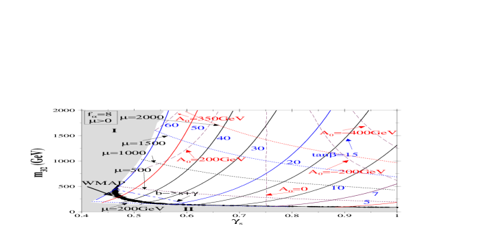
(a) Contours of constant $\tan\beta$, $A_{0}$ and $\mu$ are shown on the available parameter space for $\mu>0$ in the $(\gamma_{s}-m_{3/2})$ plane. The $b\rightarrow s+\gamma$ contour is shown as a dot-dashed line below which the region is disallowed. WMAP satisfied relic density region is shown as small shaded area in black. The gray region-I refers to the discarded zone of very large $\tan\beta$ where Yukawa couplings are beyond the perturbative domain. The gray region II results from the absence of REWSB or smaller $m_{\tilde{\chi}_{1}^{\pm}}$ below the experimental limit.

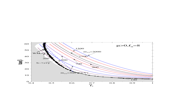
(b) The contours of constant $m_{3/2}$ in the $\gamma_{s}-\tan\beta$ plane for $\mu>0$ are as labelled. The $b\rightarrow s+\gamma$ disallowed region is in the left of the blue dashed line. The WMAP allowed region is shown in narrow shaded area in black.

Figure 1:

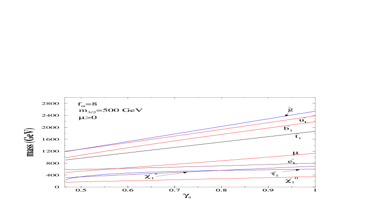
(a) Variation of sparticle masses with respect to $\gamma_{s}$ when $m_{3/2}$ is fixed at 500 GeV for $\mu>0$. The WMAP constraint is not exhibited.

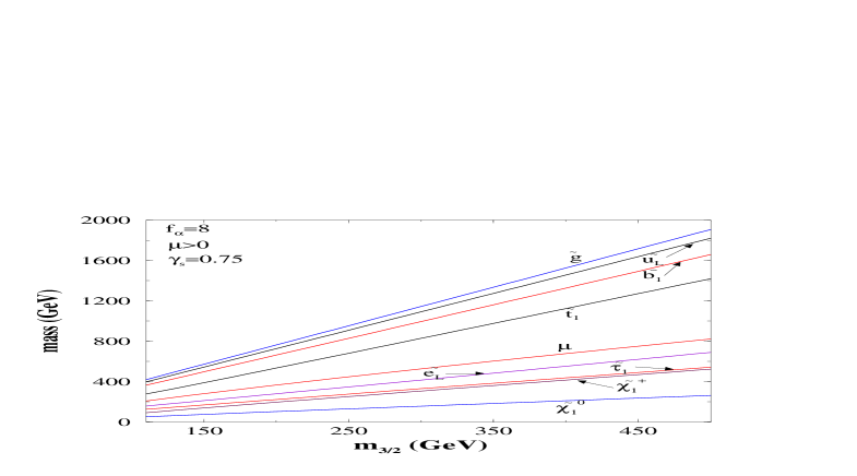
(b) Variation of sparticle masses with respect to $m_{3/2}$ when $\gamma_{s}$ is fixed at 0.75 for $\mu>0$. The WMAP constraint is not exhibited.

Figure 2:

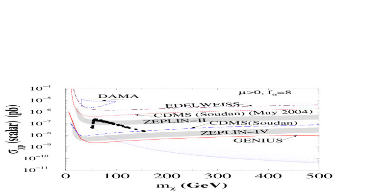
(a) Scatter plot for spin independent LSP-proton cross section vs LSP mass for $\mu>0$ when $\gamma_{s}$ and $m_{3/2}$ are scanned. The region with black circles satisfies the WMAP constraint. Present limits (top three contours) and future accessibility regions are shown.

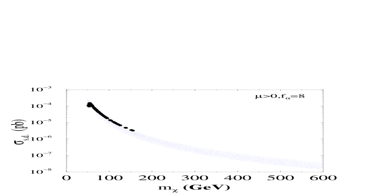
(b) Spin-dependent LSP-proton cross section vs LSP mass for $\mu>0$. The region with black circles satisfies the WMAP constraint.

Figure 3:

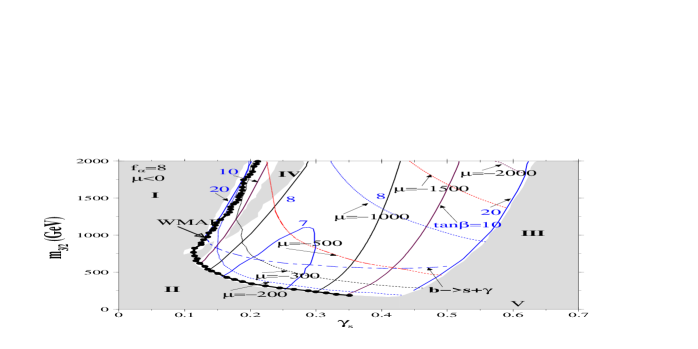
(a) Contours of constant $\tan\beta$, and $\mu$ are shown on the available parameter space for $\mu<0$ in the $(\gamma_{s}-m_{3/2})$ plane. The $b\rightarrow s+\gamma$ contour is shown as a dot-dashed line below which the region is disallowed. WMAP satisfied relic density region is shown as small shaded area in black. The disallowed gray region I and III are typically discarded because of the absence of consistent GUT scale inputs. The region II typically refers to absence of REWSB or smaller than experimental lower limits of $m_{\tilde{\chi}_{1}^{\pm}}$. The region IV is a no solution zone like I and III, but its location and extent depends on the sensitivity of the minimization scale for REWSB. Region V is the tachyonic $\tilde{\tau}_{1}$ zone.

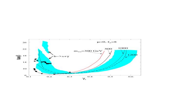
(b) The contours of constant $m_{3/2}$ in the $\gamma_{s}-\tan\beta$ plane for $\mu<0$ are as labelled. The shaded (cyan) regions satisfy the $b\rightarrow s+\gamma$ limits. The black dotted area does not satisfy $b\rightarrow s+\gamma$ limits. The WMAP allowed region is shown in filled circles in black.

Figure 4:

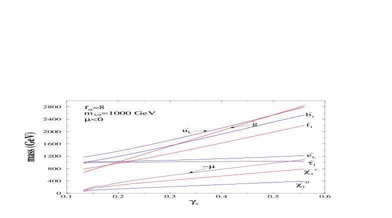
(a) Variation of sparticle masses with respect to $\gamma_{s}$ when $m_{3/2}$ is fixed at 1000 GeV for $\mu<0$. The WMAP constraint is not exhibited.

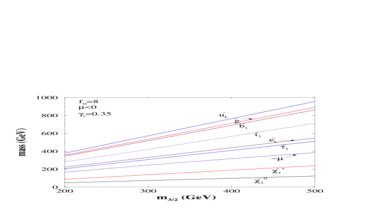
(b) Variation of sparticle masses with respect to $m_{3/2}$ when $\gamma_{s}$ is fixed at 0.35 for $\mu<0$. The WMAP constraint is not exhibited.

Figure 5:

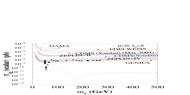
(a) Scatter plot for spin independent LSP-proton cross section vs LSP mass for $\mu<0$ when $\gamma_{s}$ and $m_{3/2}$ are scanned. The region with black circles satisfies the WMAP constraint. Present limits (top three contours) and future accessibility regions are shown.

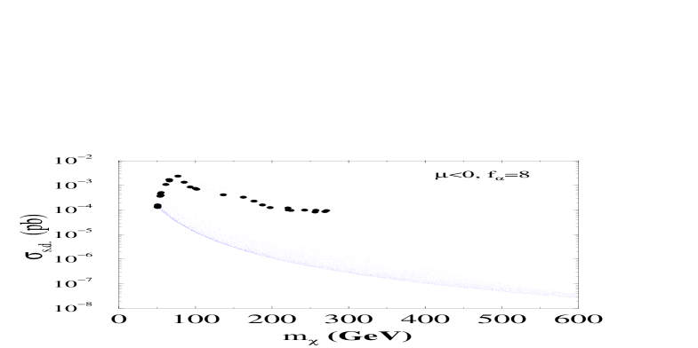
(b) Spin-dependent LSP-proton cross section vs LSP mass for $\mu<0$. The region with black circles satisfies the WMAP constraint.

Figure 6:

(a) Analysis at the self dual point $f_{\alpha}=3\sqrt{3}$ where contours of constant $\tan\beta$ are shown on the available parameter space for $\mu>0$ in the $(\gamma_{s}-m_{3/2})$ plane. The $b\rightarrow s+\gamma$ contour is shown as a dot-dashed line below which the region is disallowed. WMAP satisfied relic density region is shown as small shaded area in black. The gray region-I refers to the discarded zone of very large $\tan\beta$ where Yukawa couplings are beyond the perturbative domain. The gray region II results from the absence of REWSB or smaller $m_{\tilde{\chi}_{1}^{\pm}}$ below the experimental limit.

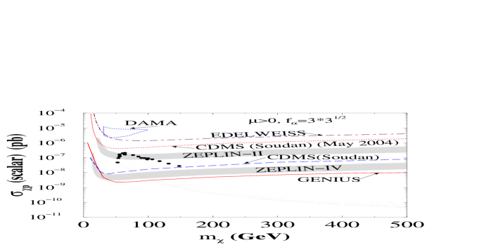
(b) Analysis at the self dual point $f_{\alpha}=3\sqrt{3}$ where a scatter plot for spin independent LSP-proton cross section vs LSP mass for $\mu>0$ is shown when $\gamma_{s}$ and $m_{3/2}$ are scanned. The region with black circles satisfies the WMAP constraint. Present limits (top three contours) and future accessibility regions are shown.

Figure 7:

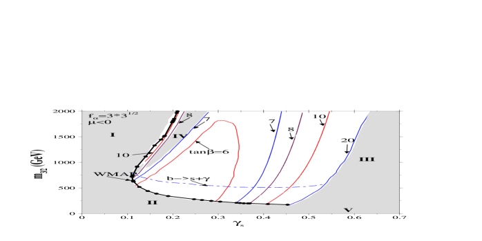
(a) Analysis at the self dual point $f_{\alpha}=3\sqrt{3}$ where contours of constant $\tan\beta$ are shown on the available parameter space for $\mu<0$ in the $(\gamma_{s}-m_{3/2})$ plane. The $b\rightarrow s+\gamma$ contour is shown as a dot-dashed line below which the region is disallowed. WMAP satisfied relic density region is shown as small shaded area in black. The disallowed regions I to V are same as those in Fig.(4(a)).

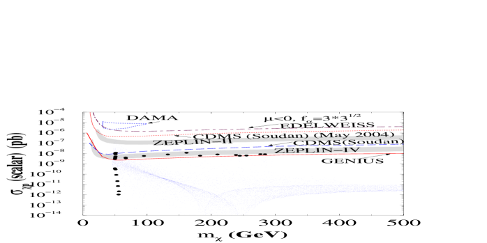
(b) Analysis at the self dual point $f_{\alpha}=3\sqrt{3}$ where a scatter plot for spin independent LSP-proton cross section vs LSP mass for $\mu<0$ is shown when $\gamma_{s}$ and $m_{3/2}$ are scanned. The region with black circles satisfies the WMAP constraint. Present limits (top three contours) and future accessibility regions are shown.

Figure 8:

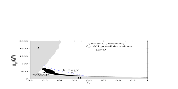
(a) Composite analysis for relic density and $Br(b\rightarrow s+\gamma)$ in $(\gamma_{s}-m_{3/2})$ plane for $\mu>0$ with the inclusion of $U_{i}$ moduli at the self dual points corresponding to all possible values of $f_{\alpha}:2^{n}3^{3-n/2},n=0,...6$. The $b\rightarrow s+\gamma$ contour is shown as a dot-dashed line below which the region is maximally disallowed. WMAP satisfied relic density region is maximally shown as small shaded area in black. The gray areas are similar to the discarded regions of Fig.(1(a)).

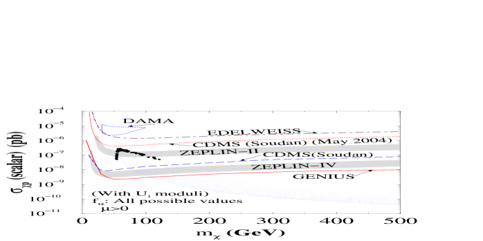
(b) Scatter plot for spin independent LSP-proton cross section vs LSP mass for $\mu>0$ when $\gamma_{s}$ and $m_{3/2}$ are scanned, for the composite analysis with $U_{i}$ moduli corresponding to Fig.(9(a)). The region with black circles satisfies the WMAP constraint.

Figure 9:

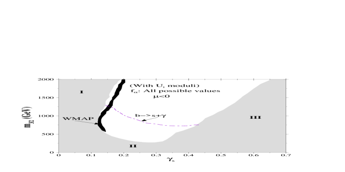
(a) Composite analysis for relic density and $Br(b\rightarrow s+\gamma)$ in $(\gamma_{s}-m_{3/2})$ plane for $\mu<0$ with the inclusion of $U_{i}$ moduli at the self dual points corresponding to all possible values of $f_{\alpha}:2^{n}3^{3-n/2},n=0,...6$. The $b\rightarrow s+\gamma$ contour is shown as a dot-dashed line below which the region is maximally disallowed. WMAP satisfied relic density region is maximally shown as small shaded area in black. The gray areas are similar to the discarded regions of Fig.(4(a)).

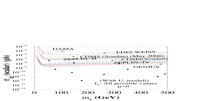
(b) Scatter plot for spin independent LSP-proton cross section vs LSP mass for $\mu<0$ when $\gamma_{s}$ and $m_{3/2}$ are scanned, for the composite analysis with $U_{i}$ moduli corresponding to Fig.(10(a)). A few scattered points shown in black circles satisfies the WMAP constraint. Most of such points corresponds to ${\tilde{m}}_{\chi^{0}_{1}}>>500$ GeV, thus falling outside the displayed limit.

Figure 10:

References

- [1] C. L. Bennett et al., Astrophys. J. Suppl. 148, 1 (2003), [arXiv:astro-ph/0302207].
- [2] D. N. Spergel et al., Astrophys. J. Suppl. 148, 175 (2003), [arXiv:astro-ph/0302209].
- [3] U. Chattopadhyay, A. Corsetti and P. Nath, Phys. Rev. D 68, 035005 (2003) [arXiv:hep-ph/0303201].
- [4] J. Ellis, K. A. Olive, Y. Santoso and V. C. Spanos, Phys. Lett. B565, 176, (2003), [arXiv:hep-ph/0303043]; H. Baer and C. Balazs, JCAP 0305, 006 (2003), [arXiv:hep-ph/0303114]; A. B. Lahanas and D. V. Nanopoulos, Phys. Lett. B568, 55, (2003) [arXiv:hep-ph/0303130].
- [5] H. Baer, C. Balazs, A. Belyaev and J. O’Farrill, JCAP 0309, 007 (2003), [arXiv:hep-ph/0305191]; H. Baer, C. Balazs, A. Belyaev, T. Krupovnickas and X. Tata, JHEP 0306, 054 (2003) [arXiv:hep-ph/0304303]; R. Arnowitt, B. Dutta and B. Hu, arXiv:hep-ph/0310103; J. R. Ellis, K. A. Olive, Y. Santoso and V. C. Spanos, Phys. Lett. B 573, 162 (2003) [arXiv:hep-ph/0305212]; J.D. Vergados, P. Quentin and D. Strottman, hep-ph/0310365.
- [6] For a review see, U. Chattopadhyay, A. Corsetti and P. Nath, arXiv:hep-ph/0310228; A. B. Lahanas, N. E. Mavromatos and D. V. Nanopoulos, Int. J. Mod. Phys. D 12, 1529 (2003) [arXiv:hep-ph/0308251].
- [7] K. L. Chan, U. Chattopadhyay and P. Nath, Phys. Rev. D 58, 096004 (1998) [arXiv:hep-ph/9710473];. J. L. Feng, K. T. Matchev and T. Moroi, Phys. Rev. D 61, 075005 (2000).
- [8] P. Nath and T. R. Taylor, Phys. Lett. B 548, 77 (2002) [arXiv:hep-ph/0209282].
- [9] For a sample of heterotic string models see, L.E.Ibanez, H. P. Nilles and F. Quevedo, Nucl. Phys. B307, 109 (1988); A. Antoniadis, J.Ellis, J. Hagelin, and D.V. Nanopoulos, Phys. Lett. B194, 231(1987); B. R. Green, K. H. Kirklin, P.J. Miron G.G. Ross, Nucl. Phys.B292, 606(1987); R. Arnowitt and P. Nath, Phys. Rev. D40, 191(1989); A. H. Chamseddine and M. Quiros, Nucl. Phys. B 316, 101(1989); D.C. Lewellen, Nucl. Phys. B337, 61(1990); A. Farragi, Phys. Lett. B278, 131(1992); S. Chaudhuri, S.-W. Chung, G. Hockney, and J.D. Lykken, Nucl. Phys.452, 89(1995); G.B. Cleaver, Nucl. Phys. B456, 219(1995); M. Cvetic and P. Langacker, Phys. Rev. D54, 3570(1996); Z. Kakushadze and S.H.H. Tye, Phys. Rev. D55, 7896(1997).
- [10] S. Ferrara, N. Magnoli, T. R. Taylor and G. Veneziano, Phys. Lett. B 245, 409(1990); A. Font, L. E. Ibanez, D. Lüst and F. Quevedo, Phys. Lett. B 245, 401(1990); H. P. Nilles and M. Olechowski, Phys. Lett. B 248, 268(1990); P. Binetruy and M. K. Gaillard, Phys. Lett. B 253, 119(1991); M. Cvetic, A. Font, L. E. Ibanez, D. Lüst and F. Quevedo, Nucl. Phys. B 361, 194(1991).
- [11] A. Brignole, L. E. Ibanez, C. Munoz and C. Scheich, Z. Phys. C 74, 157 (1997); B. de Carlos, J. A. Casas and C. Munoz, Nucl. Phys. B 399, 623(1993); A. Brignole, L. E. Ibanez and C. Munoz, Phys. Lett. B 387,769(1996).
- [12] H. P. Nilles, Phys. Lett. B 115, 193(1982); S. Ferrara, L. Girardello and H. P. Nilles, Phys. Lett. B 125, 457(1983); M. Dine, R. Rohm, N. Seiberg and E. Witten, Phys. Lett. B 156, 55(1985); C. Kounnas and M. Porrati, Phys. Lett. B 191, 91(1987).
- [13] P. Binetruy, M. K. Gaillard and B. D. Nelson, Nucl. Phys. B 604, 32(2001); M. K. Gaillard, B. D. Nelson and Y. Y. Wu, Phys. Lett. B 459, 549(1999); M. K. Gaillard and J. Giedt, Nucl. Phys. B 636, 365(2002).
- [14] G. L. Kane, J. Lykken, S. Mrenna, B. D. Nelson, L. T. Wang and T. T. Wang, Phys. Rev. D 67, 045008 (2003) [arXiv:hep-ph/0209061]; B. C. Allanach, S. F. King and D. A. J. Rayner, arXiv:hep-ph/0403255.
- [15] A. H. Chamseddine, R. Arnowitt and P. Nath, Phys. Rev. Lett. 49, 970(1982); R. Barbieri, S. Ferrara and C. A. Savoy, Phys. Lett. B 119, 343(1982). L. Hall, J. Lykken, and S. Weinberg, Phys. Rev. D 27, 2359 (1983): P. Nath, R. Arnowitt and A.H. Chamseddine, Nucl. Phys. B 227, 121 (1983); P. Nath, “Twenty years of SUGRA,” arXiv:hep-ph/0307123.
- [16] G. Lopes Cardoso and B. A. Ovrut, Nucl. Phys. B 369, 351(1992); J. P. Derendinger, S. Ferrara, C. Kounnas and F. Zwirner, Nucl. Phys. B 372, 145(1992); I. Antoniadis, E. Gava, K. S. Narain and T. R. Taylor, Nucl. Phys. B 407, 706(1993).
- [17] A. B. Lahanas and D. V. Nanopoulos, Phys. Rept. 145, 1 (1987).
- [18] U. Chattopadhyay and P. Nath, Phys. Rev. D 66, 093001 (2002) [arXiv:hep-ph/0208012].and references therein.
- [19] G. W. Bennett et al. [Muon g-2 Collaboration], Phys. Rev. Lett. 92, 161802 (2004) [arXiv:hep-ex/0401008].
- [20] I. Antoniadis, E. Gava, K. S. Narain and T. R. Taylor, Nucl. Phys. B 432, 187 (1994) [arXiv:hep-th/9405024].
- [21] R. Arnowitt and P. Nath, Phys. Rev. Lett. 69, 725(1992).
- [22] P. Nath and R. Arnowitt, Phys. Lett. B 336, 395 (1994); Phys. Rev. Lett. 74, 4592 (1995); F. Borzumati, M. Drees and M. Nojiri, Phys. Rev. D 51, 341 (1995); H. Baer, M. Brhlik, D. Castano and X. Tata, Phys. Rev. D 58, 015007 (1998).
- [23] H. Baer, A. Belyaev, T. Krupovnickas and A. Mustafayev, arXiv:hep-ph/0403214; K. i. Okumura and L. Roszkowski, Journal of High Energy Physics, 0310, 024 (2003) [arXiv:hep-ph/0308102]; M. Carena, D. Garcia, U. Nierste, C.E.M. Wagner, Phys. Lett. B499 141 (2001); G. Degrassi, P. Gambino, G.F. Giudice, JHEP 0012, 009 (2000); M. Ciuchini, G. Degrassi, P. Gambino and G. F. Giudice, Nucl. Phys. B 534, 3 (1998).
- [24] P. Gambino and M. Misiak, Nucl. Phys. B611, 338 (2001); P. Gambino and U. Haisch, JHEP 0110, 020 (2001); A.L. Kagan and M. Neubert, Eur. Phys. J. C7, 5(1999). A.L. Kagan and M. Neubert, Eur. Phys. J. C27, 5(1999).
- [25] K. Abe et al. [Belle Collaboration], Phys. Lett. B 511, 151 (2001) [arXiv:hep-ex/0103042]; S. Chen et.al. (CLEO Collaboration), Phys. Rev. Lett. 87, 251807 (2001); R. Barate et al. [ALEPH Collaboration], Phys. Lett. B 429, 169 (1998).
- [26] R. Abusaidi et.al., Phys. Rev. Lett.84, 5699(2000), ”Exclusion Limits on WIMP-Nucleon Cross-Section from the Cryogenic Dark Matter Search”, CDMS Collaboration preprint CWRU-P5-00/UCSB-HEP-00-01 and astro-ph/0002471.
- [27] H.V. Klapdor-Kleingrothaus, et.al., ”GENIUS, A Supersensitive Germanium Detector System for Rare Events: Proposal”, MPI-H-V26-1999, hep-ph/9910205; H. V. Klapdor-Kleingrothaus, “Search for dark matter by GENIUS-TF and GENIUS,” Nucl. Phys. Proc. Suppl. 110, 58 (2002) [arXiv:hep-ph/0206250].
- [28] D. Cline, “Status of the search for supersymmetric dark matter,” arXiv:astro-ph/0306124.
- [29] D. R. Smith and N. Weiner, Nucl. Phys. Proc. Suppl. 124, 197 (2003) [arXiv:astro-ph/0208403].
- [30] [CDMS Collaboration], “First Results from the Cryogenic Dark Matter Search in the Soudan Underground Lab,” arXiv:astro-ph/0405033.
- [31] G. Chardin et al. [EDELWEISS Collaboration], Nucl. Instrum. Meth. A 520, 101 (2004); A. Benoit et al., Phys. Lett. B545, 43 (2002), [arXiv:astro-ph/0206271].
- [32] R. Bernabei et al. [DAMA Collaboration], Phys. Lett. B 480, 23 (2000).
- [33] U. Chattopadhyay, A. Corsetti and P. Nath, Phys. Rev. D 66, 035003 (2002) [arXiv:hep-ph/0201001]; M. E. Gomez, G. Lazarides and C. Pallis, Phys. Rev. D 61, 123512 (2000) [arXiv:hep-ph/9907261].
- [34] U. Chattopadhyay and D. P. Roy, Phys. Rev. D 68, 033010 (2003) [arXiv:hep-ph/0304108].
- [35] H. Baer, A. Belyaev, T. Krupovnickas and X. Tata, JHEP 0402, 007 (2004) [arXiv:hep-ph/0311351].
- [36] P. Binetruy, Y. Mambrini and E. Nezri, arXiv:hep-ph/0312155.
- [37] M. E. Gomez, T. Ibrahim, P. Nath and S. Skadhauge, arXiv:hep-ph/0404025; T. Nihei and M. Sasagawa, arXiv:hep-ph/0404100; M. Argyrou, A. B. Lahanas, D. V. Nanopoulos and V. C. Spanos, arXiv:hep-ph/0404286.
- [38] C. Munoz, arXiv:hep-ph/0309346.
- [39] R. Blumenhagen, B. Körs, D. Lüst and T. Ott, Nucl. Phys. B 616, 3(2001). [hep-th/0107138].
- [40] L. E. Ibanez, F. Marchesano and R. Rabadan, JHEP 0111, 002(2001) [hep-th/0105155].
- [41] M. Cvetic, G. Shiu and A. M. Uranga, Phys. Rev. Lett. 87, 201801(2001) [hep-th/0107143].
- [42] B. Kors and P. Nath, Nucl. Phys. B 681, 77 (2004) [arXiv:hep-th/0309167].
- [43] M. Grana, T. W. Grimm, H. Jockers and J. Louis, arXiv:hep-th/0312232.
- [44] L. Anchordoqui, H. Goldberg and P. Nath, arXiv:hep-ph/0403115 (To appear in Phys. Rev. D).