Adler function and hadronic contribution to the muon $g-2$ in a nonlocal chiral quark model

1 Introduction

The transition from perturbative regime of QCD to nonperturbative one has yet remained under discussion. At high momenta the fundamental degrees of freedom are almost massless asymptotically free quarks. At low momenta the nonperturbative regime is adequately described in terms of constituent quarks with masses dynamically generated by spontaneous breaking of chiral symmetry. The instanton model of QCD vacuum [1] provides the mechanism of dynamical quark dressing in the background of instanton vacuum and leads to generation of the momentum dependent quark mass that interpolates these two extremes. Still it is not clear how an intuitive picture of this transition may be tested at the level of observables. In this paper we demonstrate that the Adler function depending on spacelike momenta may serve as the appropriate quantity. This function defined as the logarithmic derivative of the current-current correlator can be extracted from the experimental data of ALEPH [2] and OPAL [3] collaborations on inclusive hadronic $\tau$ decays. From theoretical point of view it is well known that in high-energy asymptotically free limit the Adler function calculated for massless quarks is a nonzero constant. From the other side in the constituent quark model (suitably regularized) this function is zero at zero virtuality. Thus the transition of the Adler function from its constant asymptotic behaviour to zero is very indicative concerning the nontrivial QCD dynamics at intermediate momenta. In this paper we intend to show that the instanton-like nonlocal chiral quark model (N$\chi$QM) describes this transition correctly. In particular, we analyze the correlator of vector currents and corresponding Adler function in the framework of N$\chi$QM that allows us to draw a precise and unambiguous comparison of the experimental data with the model calculations. The use in the calculations of a covariant nonlocal low-energy quark model based on the self-consistent approach to the dynamics of quarks has many attractive features as it preserves the gauge invariance, is consistent with the low-energy theorems, as well as takes into account the large-distance dynamics controlled by the bound states. As an application we estimate the leading order hadronic vacuum polarization contribution to the muon anomalous magnetic moment which is expressed as an convolution integral over spacelike momenta of the Adler function and confront it with the recent results of the measurements by the Muon $\left(g-2\right)$ collaboration [4].

The paper is organized as follows. In Sect. 2, we briefly recall the definition of the Adler function and the way how to extract it from the experimental data. Then in Sect. 3 we remind the definition of the leading order contribution of hadronic vacuum polarization to the muon anomalous magnetic moment and present its phenomenological estimates. In Sect. 4 and 5 we outline the gauged nonlocal chiral quark model extended by inclusion of the vector and axial-vector mesons and derive the expressions for the Adler function within the model considered. Then, after fixing the model parameters in Sect. 6, we confront the model results with available experimental data on the Adler function and the $V-A$ correlator in Sects. 7 and 8, correspondingly. Sect. 9 contains our conclusions. In Appendices we give necessary information about the nonlocal vertices of quark interaction with external currents, phenomenology of vector mesons and the structure of non-chiral corrections to low energy observables.

2 The Adler function

In the chiral limit, where the masses of $u$, $d$, $s$ light quarks are set to zero, the vector ($V$) and non-singlet axial-vector ($A$) current-current correlation functions in the momentum space (with $-q^{2}\equiv Q^{2}\geq 0$) are defined as

$$\Pi_{\mu\nu}^{J,ab}(q) =i\int d^{4}x~{}e^{iqx}\Pi_{\mu\nu}^{J,ab}(x)=\,\left(q_{\mu}q_{\nu}-g_{\mu\nu}q^{2}\right)\Pi_{J}(Q^{2})\delta^{ab},$$ (1)

$$\qquad\Pi_{\mu\nu}^{J,ab}(x) =\langle 0\left|T\left\{J_{\mu}^{a}(x)J_{\nu}^{b}(0)^{\dagger}\right\}\right|0\rangle,$$

where the QCD $V$ and $A$ currents are

$$J_{\mu}^{a}=\overline{q}\gamma_{\mu}\frac{\lambda^{a}}{\sqrt{2}}q,\qquad J_{\mu}^{5a}=\overline{q}\gamma_{\mu}\gamma_{5}\frac{\lambda^{a}}{\sqrt{2}}q,$$ (2)

and $\lambda^{a}$ are Gell-Mann matrices $\left(\mathrm{tr}\lambda^{a}\lambda^{b}=2\delta^{ab}\right)$. The momentum-space two-point correlation functions obey (suitably subtracted) dispersion relations,

$$\Pi_{J}(Q^{2})=\int_{0}^{\infty}\frac{ds}{s+Q^{2}}\frac{1}{\pi}\mathrm{Im}\Pi_{J}(s),$$ (3)

where the imaginary parts of the correlators determine the spectral functions

$$\rho_{J}(s)=4\pi\mathrm{\operatorname{Im}}\Pi_{J}(s+i0).$$

Instead of the correlation function it is more convenient to work with the Adler function defined as

$$D_{J}(Q^{2}){=-Q}^{2}\frac{d\Pi_{J}(Q^{2})}{dQ^{2}}{\,=}\frac{1}{4\pi^{2}}\int_{0}^{\infty}{dt}\frac{Q^{2}}{(t+Q^{2})^{2}}{\,\rho_{J}(t)\,.}$$ (4)

Recently, the isovector $V$ and $A$ spectral functions have been determined separately with high precision by the ALEPH [2] and OPAL [3] collaborations from the inclusive hadronic $\tau$-lepton decays ($\tau\rightarrow\nu_{\tau}+$ hadrons) in the interval of invariant masses up to the $\tau$ mass, $0\leq s\leq m_{\tau}^{2}$. It is important to note that the experimental separation of the $V$ and $A$ spectral functions allows us to test accurately the saturation of the chiral sum rules of Weinberg-type in the measured interval. On the other hand, at large $s$ the correlators can be confronted with perturbative QCD (pQCD) thanks to sufficiently large value of the $\tau$ mass.

Figure 1: The isovector vector spectral function from hadronic $\tau$- decays [2]. The dashed line is the asymptotic freedom prediction, $1/(4\pi^{2}).$

Figure 2: The vector Adler function constructed with use of LO (dot-dashed), NLO (dotted) and NNLO (full line) pQCD asymptotics. The dashed line is asymptotic freedom prediction, $1/4\pi^{2}$.

The vector spectral function and the corresponding Adler function determined from the ALEPH data (see below) are shown in Figs. 2 and 2. The behaviour of the correlators at low and high momenta is constrained by QCD. In the regime of large momenta the Adler function is dominated by pQCD contribution supplemented by small power corrections

$$D_{V}(Q^{2}\rightarrow\infty)=D_{V}^{\mathrm{pQCD}}(Q^{2})-\frac{\alpha_{s}}{4\pi^{3}}\frac{\lambda^{2}}{Q^{2}}+\frac{1}{6}\frac{\alpha_{s}}{\pi}\frac{\left\langle\left(G_{\mu\nu}^{a}\right)^{2}\right\rangle}{Q^{4}}+\frac{O_{D}^{6}}{Q^{6}}+\mathcal{O}(\frac{1}{Q^{8}}),$$ (5)

where the pQCD contribution with three-loop accuracy is given in the chiral limit in $\overline{\mathrm{MS}}$ renormalization scheme by [5, 6]

$$D_{V}^{\mathrm{pQCD}}(Q^{2};\mu^{2})={\frac{1}{4\pi^{2}}}\left\{1+\frac{\alpha_{s}\left(\mu^{2}\right)}{\pi}+\left[F_{2}-\beta_{0}\ln{\frac{Q^{2}}{\mu^{2}}}\right]\left(\frac{\alpha_{s}(\mu^{2})}{\pi}\right)^{2}\right.+$$ (6)

$${+}\left.\left[F_{3}-\left({2}F_{2}\beta_{0}{+\beta_{1}}\right){\ln{\frac{Q^{2}}{\mu^{2}}}+\beta_{0}^{2}}\left(\frac{\pi^{2}}{3}{+\ln}^{2}{{\frac{Q^{2}}{\mu^{2}}}}\right)\right]\left(\frac{\alpha_{s}(\mu^{2})}{\pi}\right)^{3}{+}\mathcal{O}{(\alpha}_{s}^{4}{)}\right\}$$

where

$$\beta_{0}{=}\frac{1}{4}\left(11{-}\frac{2}{3}n_{f}\right){\,,\qquad}\beta_{1}{=}\frac{1}{8}\left(51{-}\frac{19}{3}{n}_{f}\right){\,,}$$

$$F_{2}{=1.98571-0.115295\,n}_{f}{\,,\qquad}F_{3}{=-6.63694-1.20013\,n}_{f}{-0.00518\,n}_{f}^{2}{\,,}$$

with $\alpha_{s}(Q^{2})$ being the solution of the equation

$$\frac{\pi}{\beta_{0}\alpha_{s}(Q^{2})}-\frac{\beta_{1}}{\beta_{0}^{2}}\ln\left[\frac{\pi}{\beta_{0}\alpha_{s}(Q^{2})}+\frac{\beta_{1}}{\beta_{0}^{2}}\right]=\ln\frac{Q^{2}}{\Lambda^{2}}\,.$$ (7)

In (5) along with standard power corrections due to the gluon and quark condensates we include the unconventional term suppressed as, $\sim 1/Q^{2}$. Its appearance was augmented in [7] and also found in the N$\chi$QM [8].

In the low-$Q^{2}$ limit it is only rigorously known from the theory that

$${D}_{V}{(Q}^{{2}}{\rightarrow 0)=Q}^{{2}}{D}_{V}^{\prime}{(0)+}\mathcal{O}{(Q}^{4}{).}$$ (8)

It is clear (see also Fig. 2) that the Adler function is very sensitive to transition between asymptotically free (almost massless current quarks) region described by (5), (6) to the hadronic regime with almost constant constituent quarks where one has (8).

To extract the Adler function from experimental data supplemented by QCD asymptotics (5), (6) we take following [9] an ansatz for the hadronic spectral functions in the form

$$\rho_{J}\left(t\right)=\rho_{\mathrm{J}}^{\mathrm{ALEPH}}\left(t\right)\theta(s_{0}-t)+\rho_{J}^{\mathrm{pQCD}}\left(t\right)\theta(t-s_{0})\,\,,$$ (9)

where

$$\frac{1}{4\pi^{2}}\rho_{V}^{\mathrm{pQCD}}\left(t\right)=D_{V}^{\mathrm{pQCD}}\left(t\right)-\frac{121\pi^{2}}{48}\left(\frac{\alpha_{s}(t)}{\pi}\right)^{3},$$ (10)

and find the value of continuum threshold $s_{0}$ from the global duality interval condition:

$$\int_{0}^{s_{0}}dt\,\rho_{\mathrm{J}}^{\mathrm{ALEPH}}(t)=\int_{0}^{s_{0}}dt\rho_{J}^{\mathrm{pQCD}}\,(t)\,.$$ (11)

Using the experimental input corresponding to the $\tau$–decay data and the pQCD expressions

$$\frac{1}{4\pi^{2}}\int_{0}^{s_{0}}dt\,\rho_{V}^{\mathrm{pQCD}}(t) =\frac{N_{c}}{12\pi^{2}}s_{0}\left\{1+\frac{\alpha_{\mathrm{s}}(s_{0})}{\pi}+\left[F_{2}+\beta_{0}\right]\left(\frac{\alpha_{\mathrm{s}}(s_{0})}{\pi}\right)^{2}+\right.$$ (12)

$$\left.+\left[F_{3}+\left(2F_{2}\beta_{0}+\beta_{1}\right)+2\beta_{0}^{2}\right]\left(\frac{\alpha_{\mathrm{s}}(s_{0})}{\pi}\right)^{3}\right\},$$

$$\rho_{V-A}^{\mathrm{pQCD}}(t)\, =0,$$ (13)

one finds (see Figs. 4 and 4) that matching between the experimental data and theoretical predictions occurs approximately at scale $s_{0}\approx 2.5\mathrm{GeV}^{2}$. Note that the condition (13) in the $V-A$ channel corresponds to matching the second Weinberg chiral sum rule.

Figure 3: The integral, Eq. (11), versus the upper integration limit, $s_{0}$, for the $V$ spectral density. The integral of the experimental data corresponds to solid line and the pQCD prediction (12) is given by the dashed line.

Figure 4: The integral, Eq. (11), versus the upper integration limit, $s_{0}$, for the $V-A$ spectral density (second Weinberg sum rule). The pQCD prediction is given by dashed line, and the experimental function is given by solid line.

The vector Adler function (4) obtained from matching the low momenta experimental data and high momenta pQCD asymptotics by using the spectral density (9) is shown in Fig. 2, where we use the pQCD asymptotics (10) of the massless vector spectral function to four loops with $\Lambda_{\overline{\mathrm{MS}}}^{n_{f}=3}=372$ MeV and choose the matching parameter as $s_{0}=2.5$ GeV${}^{-1}.$ Admittedly, in the Euclidean presentation of the data the detailed resonance structure corresponding to the $\rho$ and $a_{1}$ mesons seen in the Minkowski region (Fig. 2) is smoothed out, hence the verification of the theory is not as stringent as would be directly in the Minkowski space.

3 Leading order hadronic vacuum polarization contributions.

The anomalous magnetic moment of the muon is known to an unprecedented accuracy of order of $1$ ppm. The latest result from the measurements of the Muon $(g-2)$ collaboration at Brookhaven is [4]

$$a_{\mu}\equiv{\frac{1}{2}}(g_{\mu}-2)=11\ 659\ 208\left(6\right)\cdot 10^{-10}.$$ (14)

Using $e^{+}e^{-}$ annihilation data and data from hadronic $\tau$ decays the standard model predictions are [10, 11]

$$a_{\mu}^{SM}=\left\{\begin{array}[l]{l}11\ 659\ 181\left(8\right)\cdot 10^{-10}\qquad e^{+}e^{-},\\ 11\ 659\ 196\left(7\right)\cdot 10^{-10}\qquad\tau.\end{array}\right.$$ (15)

The difference between the experimental determination of $a_{\mu}$ and the standard model using the $e^{+}e^{-}$ or $\tau$ data for the calculation of the hadronic vacuum polarization is $2.7\sigma$ and $1.4\sigma$, respectively.

The standard model prediction for $a_{\mu}$ consists of quantum electrodynamics, weak and hadronic contributions. The QED and weak contributions to $a_{\mu}$ have been calculated with great accuracy [12]

$$a_{\mu}^{\mathrm{QED}}=11~{}658~{}471.935(0.203)\cdot 10^{-10}$$ (16)

and [13]

$$a_{\mu}^{\mathrm{EW}}=15.4(0.3)\cdot 10^{-10}.$$ (17)

The uncertainties of the standard model values in (15) are dominated by the uncertainties of the hadronic photon vacuum polarization. Thus, to confront usefully theory with the experiment requires a better determination of the hadronic contributions. In the last decade, a substantial improvement in the accuracy of the contribution from the hadronic vacuum polarization was reached. It uses, essentially, precise determination of the low energy tail of the total $e^{+}e^{-}\rightarrow$ hadrons and $\tau$ lepton decays cross-sections. The contributions of hadronic vacuum polarization at order $\alpha^{2}$ quoted in the most recent articles on the subject are given in the Table 1.

Table 1.

	$e^{+}e^{-}\cite[cite]{[\@@bibref{}{DEHZh03}{}{}]}$	$\tau\cite[cite]{[\@@bibref{}{DEHZh03}{}{}]}$	$e^{+}e^{-}\cite[cite]{[\@@bibref{}{J}{}{}]}$	$e^{+}e^{-}\cite[cite]{[\@@bibref{}{TrocYnd}{}{}]}$	$\tau\cite[cite]{[\@@bibref{}{TrocYnd}{}{}]}$
$a_{\mu}^{\mathrm{hvp}~{}\left(1\right)}\cdot 10^{10}$	$696.3\pm 9.8$	$711.0\pm 8.6$	$694.8\pm 8.6$	$693.5\pm 9.0$	$701.8\pm 8.9$

The higher-order contributions at $O(\alpha^{3})$ level to $a_{\mu}^{\mathrm{hvp}~{}\left(2\right)}$ was estimated in [15]

$$a_{\mu}^{\mathrm{hvp}~{}\left(2\right)}=-10.1(0.6)\cdot 10^{-10}$$ (18)

by using analytical kernel functions and experimental data on the $e^{+}e^{-}\rightarrow$ hadrons cross-section. In addition, there exists the $O(\alpha^{3})$ contribution to $a_{\mu}$ from the hadronic light-by-light scattering diagram, $a_{\mu}^{\mathrm{h.~{}L\times L}}$, that cannot be expressed as a convolution of experimentally accessible observables and need to be estimated from theory. The recent estimate of the hadronic light-by-light scattering contribution reads [16]

$$a_{\mu}^{\mathrm{h.~{}L\times L}}=8(4)\cdot 10^{-10}\ .$$ (19)

The latest estimate of this term is given in [17], where strong constraints on the light-by-light scattering amplitude from the short-distance QCD have been imposed, with the result $a_{\mu}^{\mathrm{h.~{}L\times L}}=13.6(2.5)\cdot 10^{-10}$.

Phenomenological estimate of the total hadronic contributions to $a_{\mu}^{\mathrm{hvp}~{}\left(2\right)}$ has to be compared with the value deduced from the $g-2$ experiment (14) and known electroweak and QED corrections

$$a_{\mu}^{\mathrm{hvp}}=720.7\left(6.0\right)\cdot 10^{-10}.$$ (20)

The agreement between the standard model prediction and the present experimental value is rather good. There is certain mismatch between the experimental and theoretical predictions for $a_{\mu}$, but in view of the inconsistencies between the evaluations based on $e^{+}e^{-}$ and $\tau$ data the conclusion about discrepancy of the experiment and standard model is certainly premature.

Figure 5: The contribution of the hadronic photon vacuum polarization to anomalous magnetic moment.

In this work we analyze the contribution of hadronic photon vacuum polarization at order $\alpha^{2}$ to $a_{\mu}^{\mathrm{hvp}}$ (Fig. 5) from the point of view of the nonlocal chiral quark model of low energy QCD and show that, within this framework, it might be possible realistically to determine this value to a sufficiently safe accuracy. We want to discuss how well this model, which has been developed in refs. [18] and [8], does in calculating $a_{\mu}^{\mathrm{hvp}~{}\left(1\right)}$. This quantity is usually expressed in the form of a spectral representation $(e^{2}=4\pi\alpha)$

$$a_{\mu}^{\mathrm{hvp}\left(1\right)}=\left(\frac{\alpha}{\pi}\right)^{2}\int_{0}^{\infty}dt\frac{1}{t}K(t)\rho_{\mathrm{V}}^{(\mathrm{H})}\left(t\right)\ ,$$ (21)

which is a convolution of the hadronic spectral function $\rho_{V}^{\mathrm{(H)}}\left(t\right)$, related to the total $e^{+}e^{-}\rightarrow\gamma^{\ast}\rightarrow$ hadrons cross-section $\sigma(t)$ by$(m_{e}\rightarrow 0)$

$$\sigma(t)=4\pi\alpha^{2}\frac{1}{t}\rho_{\mathrm{V}}^{(\mathrm{H})}\left(t\right),$$ (22)

with the QED function

$$K(t)=\int_{0}^{1}dx{\frac{x^{2}(1-x)}{x^{2}+(1-x)t/m_{\mu}^{2}}}\ ,$$ (23)

which is sharply peaked at low $t$ and decreases monotonically with increasing $t$.

For our purposes, it is convenient to express $a_{\mu}^{\mathrm{hvp}\left(1\right)}$ using the integral representation [19] in terms of the Adler function

$$a_{\mu}^{\mathrm{hvp}\left(1\right)}=\frac{4}{3}\alpha^{2}\int_{0}^{1}dx\frac{\left(1-x\right)\left(2-x\right)}{x}D_{V}\left(\frac{x^{2}}{1-x}m_{\mu}^{2}\right),$$ (24)

where the charge factor $\sum Q_{i}^{2}=2/3$, $i=u,d,s,$ is taken into account. By using the Adler function determined from experiment (4) and (9) one gets the estimate

$$a_{\mu}^{\mathrm{hvp}\left(1\right)}=7.22\cdot 10^{-8}$$ (25)

which is in a reasonable agreement with the precise phenomenological numbers quoted in Table 1. In the following we determine the Adler function and $a_{\mu}^{\mathrm{hvp}\left(1\right)}$ from the effective quark model describing the dynamics of low and intermediate energy QCD.

4 The extended nonlocal chiral quark model

The bulk of the integral in (24) is governed by the low energy behaviour of the Adler function $D_{V}(Q^{2})$. The typical momentum of the virtual photon in Fig. 5 is $Q^{2}\sim m_{\mu}^{2}$. These are momenta values much smaller than the characteristic scales of the spontaneous chiral symmetry breaking or confinement $(\simeq 1GeV)$. Therefore, the appropriate way to look at this problem is within the framework of the low energy effective field model of QCD. In the low momenta domain the effect of the nonperturbative structure of QCD vacuum become dominant. Since invention of the QCD sum rule method based on the use of the standard operator product expansion (OPE) it is common to parameterize the nonperturbative properties of the QCD vacuum by using infinite towers of the vacuum average values of the quark-gluon operators. From this point of view the nonlocal properties of the QCD vacuum result from the partial resummation of the infinite series of power corrections, related to vacuum averages of quark-gluon operators with growing dimension, and may be conventionally described in terms of the nonlocal vacuum condensates [20, 21]. This reconstruction leads effectively to nonlocal modifications of the propagators and effective vertices of the quark and gluon fields. The adequate model describing this general picture is the instanton liquid model of QCD vacuum describing nonperturbative nonlocal interactions in terms of the effective action [1]. Spontaneous breaking the chiral symmetry and dynamical generation of a momentum-dependent quark mass are naturally explained within the instanton liquid model. The $V$ and $A$ current-current correlators have been calculated in [8] in the framework of the effective chiral model with instanton-like nonlocal quark-quark interactions [18] (N$\chi$QM). In the present work we extend that analysis by inclusion into consideration of the vector and axial-vector mesons generated from resummation of quark loops.

Nonlocal effective models have an important feature which makes them advantageous over the local models, such as the well known Nambu–Jona-Lasinio model (NJL). At high virtualities the quark propagator and the vertex functions of the quark coupled to external fields reduce to the free quark propagator and to local, point-like couplings. This property allows us to straightforwardly reproduce the leading (asymptotically free) terms of the OPE. For instance, the second Weinberg sum rule is reproduced in the model [8, 22], which has not been the case of the local approaches. In addition, the intrinsic nonlocalities, inherent to the model, generate unconventional power and exponential corrections which have the same character as found in [7]. The nonlocal effective model was successively applied to the description of the data from the CLEO collaboration on the pion transition form factor in the interval of the space-like momentum transfer squared up to 8 GeV² [23]. There are several further advantages in using the nonlocal models compared to the local approaches, in particular, the model is made consistent with the gauge invariance. As we shell see below the N$\chi$QM correctly reproduces leading large $Q^{2}$ behaviour of the Adler function, while the local constituent quark model fails to describe data starting from rather low $Q^{2}$.

We start with the nonlocal chirally invariant action which describes the interaction of soft quark fields. The gluon fields have been integrated out. The corresponding gauge-invariant action for quarks interacting through nonperturbative exchanges can be expressed as [18]

$$S =\int d^{4}x\ \overline{q}(x)\gamma^{\mu}\left[i\partial_{\mu}-V_{\mu}\left(x\right)-\gamma_{5}A_{\mu}\left(x\right)\right]q(x)+$$

$$+\frac{1}{2}\sum_{i=P,V,A}G_{i}\int d^{4}X\int\prod_{n=1}^{4}d^{4}x_{n}\ f_{i}(x_{n})\left[\overline{Q}(X-x_{1},X)\Gamma_{i}Q(X,X+x_{3})\overline{Q}(X-x_{2},X)\Gamma_{i}Q(X,X+x_{4})\right],$$ (26)

where in the extended version of the model the spin-flavor structure of the interaction is given by matrix products

$$G_{i}\left(\Gamma_{i}\otimes\Gamma_{i}\right):\qquad G_{P}\left(1\otimes 1+i\gamma_{5}\tau^{a}\otimes i\gamma_{5}\tau^{a}\right);\qquad G_{V}\gamma_{\mu}\otimes\gamma_{\mu};\quad-G_{A}i\gamma_{\mu}\gamma_{5}\tau^{a}\otimes i\gamma_{\mu}\gamma_{5}\tau^{a}.$$ (27)

In Eq. (26) $\overline{q}=(\overline{u},\overline{d})$ denotes the quark flavor doublet field, $G_{i}$ are the four-quark coupling constants, and $\tau^{a}$ are the Pauli isospin matrices. The separable nonlocal kernel of the interaction determined in terms of form factors $f_{i}(x),$ with normalization $f_{i}(0)=1,$ is motivated by instanton model of QCD vacuum. The instanton model predicts the hierarchy of interactions in different channels. It is most stronger in the pseudo-scalar and scalar channels providing the spontaneous breaking of chiral symmetry. At the same time it is highly suppressed in the vector and axial-vector channels. In these channels the confinement force has to be taken into account in addition. Thus, in general we treat differently the shape of form factors $f_{i}(x)$ in different channels.

In order to make gauge-invariant form of the nonlocal action with respect to external gauge fields $V_{\mu}^{a}(x)$, we define in (26) the delocalized quark field, $Q(x)$ by using the Schwinger gauge phase factor

$$Q(x,y)=P\exp\left\{i\int_{x}^{y}dz_{\mu}V_{\mu}^{a}(z)T^{a}\right\}q(y),\qquad\overline{Q}(x,y)=Q^{\dagger}(x,y)\gamma^{0},$$ (28)

where $P$ is the operator of ordering along the integration path, with $y$ denoting the position of the quark and $x$ being an arbitrary reference point. The conserved vector and axial-vector currents in the scalar sector of the model have been derived earlier in [18, 8]. The extension of these results onto the vector sector of the model is given in Appendix A.

The dressed quark propagator, $S(p)$, is defined as

$$S^{-1}(p)=\widehat{p}-M(p),$$ (29)

with the momentum-dependent quark mass found as the solution of the gap equation

$$M(p)=M_{q}f_{P}^{2}(p),$$ (30)

where $f_{P}(p)$ is the normalized $4d$ Fourier transform of the $f_{P}(x)$. The important property of the dynamical mass is that at low virtualities passing through quark its mass is close to constituent mass, while at large virtualities it goes to current mass value.

The quark-antiquark scattering matrix in different channels is found from the Bethe-Salpeter equation as

$$\widehat{T}_{i}(q)=\frac{G_{i}}{1-G_{i}J_{i}(q)},$$ (31)

with the polarization operator

$$J_{i}(q^{2})\delta_{ab}=-i\int\frac{d^{4}k}{\left(2\pi\right)^{4}}f_{i}^{2}\left(k\right)f_{i}^{2}\left(k+q\right)Tr\left[S(k)\Gamma_{i}^{a}S\left(k+q\right)\Gamma_{i}^{b}\right].$$ (32)

The positions of mesonic bound states are determined as the poles of the scattering matrix

$$\left.\det(1-G_{i}J_{i}(q))\right|_{q^{2}=m_{M}^{2}}=0.$$ (33)

The quark-meson vertices in the pseudoscalar, vector and axial-vector channels found from the residues of the scattering matrix are $\left(k^{\prime}=k+q\right)$

$$\Gamma_{\rho,s}^{a}\left(k,k^{\prime}\right) =g_{\rho qq}\gamma_{\mu}\epsilon_{s}^{\mu}f^{V}(k)f^{V}(k^{\prime})\tau^{a},\qquad\Gamma_{\omega,s}\left(k,k^{\prime}\right)=g_{\omega qq}\gamma_{\mu}\epsilon_{s}^{\mu}f^{V}(k)f^{V}(k^{\prime}),$$ (34)

$$\Gamma_{a_{1},s}^{a}\left(k,k^{\prime}\right) =g_{a_{1}qq}\gamma_{\mu}\gamma_{5}\epsilon_{s}^{\mu}f^{V}(k)f^{V}(k^{\prime})\tau^{a},\quad\Gamma_{\pi}^{a}\left(k,k^{\prime}\right)=\left(g_{\pi qq}-\widetilde{g}_{\pi qq}\widehat{q}/m_{\pi}\right)i\gamma_{5}f^{P}(k)f^{P}(k^{\prime})\tau^{a}$$

with the quark-meson couplings found from

$$g_{Mqq}^{-2}=-\left.\frac{dJ_{i}\left(q^{2}\right)}{dq^{2}}\right|_{q^{2}=m_{M}^{2}},$$ (35)

where $m_{\mathrm{M}}$ are physical masses of the $\rho\left(\omega\right)$- and $a_{1}$-mesons. Note, that the quark-pion vertex in (34) takes into account effect of the $\pi-a_{1}$ mixing.

5 Adler function within the nonlocal chiral quark model.

Our goal is to obtain the vector current-current correlator and corresponding Adler function by using the effective instanton-like model (26) and then to estimate the leading order hadron vacuum polarization correction to muon anomalous magnetic moment $a_{\mu}$. In N$\chi$QM in the chiral limit the (axial-)vector correlators have transverse character

$$\Pi_{\mu\nu}^{J}\left(Q^{2}\right)=\left(g_{\mu\nu}-\frac{q^{\mu}q^{\nu}}{q^{2}}\right)\Pi_{J}^{\mathrm{N\chi QM}}\left(Q^{2}\right),$$ (36)

where the polarization functions are given by the sum of the dynamical quark loop, the intermediate (axial-)vector mesons and the higher order mesonic loops contributions (see Fig. 6)

$$\Pi_{J}^{\mathrm{N\chi QM}}\left(Q^{2}\right)=\Pi_{J}^{Q\mathrm{Loop}}\left(Q^{2}\right)+\Pi_{J}^{\mathrm{mesons}}\left(Q^{2}\right)+\Pi_{J}^{\chi\mathrm{Loop}}\left(Q^{2}\right).$$ (37)

Figure 6: Schematic representation of the vector polarization function (37).

The spectral representation of the polarization function consists of zero width (axial-)vector resonances $\left(\Pi_{J}^{\mathrm{mesons}}\left(Q^{2}\right)\right)$ and two-meson states $\left(\Pi_{J}^{\chi\mathrm{Loop}}\left(Q^{2}\right)\right).$ The dynamical quark loop under condition of analytical confinement has no singularities in physical space of momenta.

The dominant contribution to the vector current correlator at space-like momentum transfer is given by the dynamical quark loop which was found in [8] with the result

$$\Pi_{V}^{Q\mathrm{Loop}}\left(Q^{2}\right) =\frac{4N_{c}}{Q^{2}}\int\frac{d^{4}k}{\left(2\pi\right)^{4}}\frac{1}{D_{+}D_{-}}\left\{M_{+}M_{-}+\left[k_{+}k_{-}-\frac{2}{3}k_{\perp}^{2}\right]_{ren}\right.$$ (38)

$$+\left.\frac{4}{3}k_{\perp}^{2}\left[\left(M^{\left(1\right)}\left(k_{+},k_{-}\right)\right)^{2}\left(k_{+}k_{-}-M_{+}M_{-}\right)-\left(M^{2}\left(k_{+},k_{-}\right)\right)^{\left(1\right)}\right]\right\}+$$

$$+\frac{8N_{c}}{Q^{2}}\int\frac{d^{4}k}{\left(2\pi\right)^{4}}\frac{M\left(k\right)}{D\left(k\right)}\left[M^{\prime}\left(k\right)-\frac{4}{3}k_{\perp}^{2}M^{\left(2\right)}\left(k,k+Q,k\right)\right],$$

where the notations

$$k_{\pm}=k\pm Q/2,\qquad k_{\perp}^{2}=k_{+}k_{-}-\frac{\left(k_{+}q\right)\left(k_{-}q\right)}{q^{2}},\qquad D\left(k\right)=k^{2}+M^{2}(k),$$

$$M_{\pm}=M(k_{\pm}),\ \ \ \ \ D_{\pm}=D(k_{\pm}),$$ (39)

are used. We also introduce the finite-difference derivatives defined for an arbitrary function $F\left(k\right)$ as

$$F^{(1)}(k,k^{\prime})=\frac{F(k^{\prime})-F(k)}{k^{\prime 2}-k^{2}},\qquad F^{(2)}\left(k,k^{\prime},k^{\prime\prime}\right)=\frac{F^{(1)}(k,k^{\prime\prime})-F^{(1)}(k,k^{\prime})}{k^{\prime\prime 2}-k^{\prime 2}}.$$ (40)

In (38) the first two lines represent the contribution of the dispersive diagrams and the third line corresponds to the contact diagrams (see Fig. 7 and ref. [8] for details). The expression for $\Pi_{V}^{Q\mathrm{Loop}}\left(Q^{2}\right)$ is formally divergent and needs proper regularization and renormalization procedures which are symbolically noted by $\left[..\right]_{ren}$ for the divergent term. At the same time the corresponding Adler function is well defined and finite.

Figure 7: The dynamical quark-loop contribution is the sum of dispersive and contact terms. In the dispersive diagram $\widetilde{\Gamma}$ is the bare vertex and $\Gamma$ is the total one.

Also we have checked that there is no pole in the vector correlator as $Q^{2}\rightarrow 0$, which simply means that photon remains massless with inclusion of strong interaction. In the limiting cases the Adler function derived from Eq. (38) satisfies general requirements of QCD (see leading terms in (5), (6), and (8))

$$A_{V}^{\mathrm{N\chi QM}}\left(Q^{2}\rightarrow 0\right)=\mathcal{O}\left(Q^{2}\right),\qquad A_{V}^{\mathrm{N\chi QM}}\left(Q^{2}\rightarrow\infty\right)=\frac{N_{c}}{12\pi^{2}}+\frac{O_{2}^{V}}{Q^{2}}+\mathcal{O}\left(Q^{-4}\right).$$ (41)

The leading high $Q^{2}$ asymptotics comes from the $\left[k_{+}k_{-}-\frac{2}{3}k_{\perp}^{2}\right]_{\mathrm{ren}}$ term in (38), while the subleading asymptotics is driven by ”tachionic” term with coefficient [8]

$$O_{2}^{V}=-\frac{N_{c}}{2\pi^{2}}\int_{0}^{\infty}du\frac{uM\left(u\right)M^{\prime}\left(u\right)}{D\left(u\right)}.$$ (42)

In (42) and below we use the notations $u=k^{2}$ and $M^{\prime}(u)=dM(u)/du$.

In the extended by vector interaction model (26) one gets the corrections due to the inclusion of $\rho$ and $\omega$ mesons which appear as a result of quark-antiquark rescattering in these channels

$$\Pi_{V}^{\mathrm{mesons}}\left(Q^{2}\right)=\frac{1}{2Q^{2}}\frac{G_{V}B_{V}^{2}\left(Q^{2}\right)}{1-G_{V}J_{V}^{T}\left(Q^{2}\right)},$$ (43)

where $B_{V}\left(q^{2}\right)$ is the vector meson contribution to quark-photon transition form factor

$$B_{V}\left(Q^{2}\right)=8N_{c}i\int\frac{d^{4}k}{\left(2\pi\right)^{4}}\frac{f_{+}^{V}f_{-}^{V}}{D_{+}D_{-}}\left[M_{+}M_{-}-k_{+}k_{-}+\frac{2}{3}k_{\perp}^{2}\left(1-M^{2(1)}\left(k_{+},k_{-}\right)\right)-\frac{4}{3}k_{\perp}^{2}\frac{f_{-}f^{(1)}(k_{-},k_{+})}{D_{-}}\right],$$ (44)

and $J_{V}^{T}\left(q^{2}\right)$ is the vector meson polarization function defined in (32) with $\Gamma_{\mu}^{T}=\left(g_{\mu\nu}-q_{\mu}q_{\nu}/q^{2}\right)\gamma_{\nu}$. As a consequence of the Ward-Takahashi identity one has $B_{V}\left(0\right)=0$ as it should be.

To estimate the $\pi^{+}\pi^{-}$ and $K^{+}K^{-}$ vacuum polarization insertions (chiral loops corrections) one may use the effective meson vertices generated by the Lagrangian

$$-ie\ A_{\mu}\left(\pi^{+}\overleftrightarrow{\partial}_{\mu}\pi^{-}+K^{+}\overleftrightarrow{\partial}_{\mu}K^{-}\right)\ .$$ (45)

By using the spectral density calculated from this interaction:

$$\rho_{V}^{\chi loop}\left(t\right)={\frac{1}{12}}\left(1-{\frac{4m_{\pi}^{2}}{t}}\right)^{3/2}\Theta(t-4m_{\pi}^{2})+\left(\pi\rightarrow K\ \right),$$ (46)

one finds the contribution to the Adler function as

$$D_{V}^{\chi\mathrm{Loop}}\left(Q^{2}\right)=\frac{1}{48\pi^{2}}\left[a\left(\frac{Q^{2}}{4m_{\pi}^{2}}\right)+a\left(\frac{Q^{2}}{4m_{K}^{2}}\right)\right],$$ (47)

where

$$a\left(t\right)=\frac{1}{t}\left\{3+t-\frac{3}{2}\sqrt{\frac{t+1}{t}}\left[\operatorname{arctanh}\left(\frac{1+2t}{2\sqrt{t\left(t+1\right)}}\right)+i\frac{\pi}{2}\right]\right\}.$$ (48)

The estimate (47) of the chiral loop corrections corresponds to the point-like mesons which becomes unreliable at large $t,$ where the meson form factors has to be taken into account. This contribution corresponds to the lowest order, $O(p^{4})$, calculations in $\chi$PT, is non-leading in the formal $1/N_{c}$-expansion and provides numerically small addition. We avoid to use literally the known two-loop, $O(p^{6})$, $\chi$PT result for the chiral spectral function [24, 25], since, as it was shown there, the validity of the next-to-leading order in $p^{2}$ calculations is justified only in the short interval of invariant masses $4m_{\pi}^{2}\leq t\lesssim 0.15$ GeV${}^{2}.$ The higher-loop effects become important at higher momenta.

The resulting Adler function in N$\chi$QM is given by the sum of above contributions

$$D_{V}\left(Q^{2}\right)=D_{V}^{Q\mathrm{Loop}}\left(Q^{2}\right)+D_{V}^{\mathrm{mesons}}\left(Q^{2}\right)+D_{V}^{\chi\mathrm{Loop}}\left(Q^{2}\right).$$ (49)

6 Parameters of the extended model

First of all we need to determine the shape of nonlocal form factors in the kernel of the four-fermion interaction in (45). Within the instanton model in the zero mode approximation the function $f_{p}(p^{2})$ is expressed in terms of the modified Bessel functions. However, the screening effect modifies the instanton shape at large distances leading to the constraint instantons [26]. To take into account screening and to have also simpler analytical form for $f_{p}(p^{2})$ we shall use further the Gaussian form for the instanton profile function

$$f_{P}(p)=\exp\left(-p^{2}/\Lambda_{P}^{2}\right).$$ (50)

Moreover, it is possible to show that for practical calculations of the quantities that are defined in the space-like region the exact form of nonlocality is not very important.

At the same time the profile in the (axial-)vector channels has not to be the same as in the scalar channels. Indeed, in the instanton model in the zero mode approximation there is strong interaction in the (pseudo-)scalar channels, but there is no interaction at all in the (axial-)vector channels. It means that the mechanism that bounds quarks in these states is different from the one binding the light pseudoscalar mesons. The model also predicts that while in the scalar channels the correlation length for nonlocality is given by an instanton size, $\rho\approx 0.3$ fm, the correlation length in the vector channels is related to the distance between instanton and antiinstanton, $R\approx 1$ fm. Thus, it follows the expectation for the widths of nonlocalities in momentum space in scalar and vector channels as $\Lambda_{P}>>\Lambda_{V}$. In the present work we take the function with property of analytical confinement as the nonlocal form factor in the vector channels [27, 28]

$$f_{V}^{2}(u)=\frac{L_{V}\left(u\right)D\left(u\right)}{M_{q}^{2}\left(u+L_{V}^{2}\left(u\right)\right)},\qquad f_{V}(0)=1,$$ (51)

where

$$L_{V}\left(u\right)=\left(\frac{u/\Lambda_{V}^{2}}{\exp(u/\Lambda_{V}^{2})-1}\right)^{1/4}$$

and $\Lambda_{V}$ is the momentum space width of nonlocality in the vector channel. The function (51) has the property that it tends to zero at large positive values of $u$ and has no poles.

The N$\chi$QM can be viewed as an approximation of large-$N_{c}$ QCD where the only new interaction terms, retained after integration of the high frequency modes of the quark and gluon fields down to a nonlocality scale $\Lambda$ at which spontaneous chiral symmetry breaking occurs, are those which can be cast in the form of four-fermion operators (26), (27). The parameters of the model are then the nonlocality scales $\Lambda$ and the four-fermion coupling constants $G$.

The parameters of the model are fixed in a way typical for effective low-energy quark models. In quark models one usually fits the pion decay constant, $f_{\pi}$, to its experimental value, which in the chiral limit reduces to $86$ MeV [29]. In N$\chi$QM extended by vector interactions the constant, $f_{\pi}$, is determined by

$$f_{\pi}^{2}=\frac{N_{c}}{4\pi^{2}}\int\limits_{0}^{\infty}du\ u\frac{M^{2}(u)-uM(u)M^{\prime}(u)+u^{2}M^{\prime}(u)^{2}}{D^{2}\left(u\right)}+\frac{G_{A}j_{AP}^{2}\left(0\right)}{1-G_{A}J_{A}^{L}\left(0\right)},$$ (52)

where

$$J_{A}^{L}\left(0\right)=\frac{N_{c}}{2\pi^{2}}\int\limits_{0}^{\infty}du\ uf_{V}^{4}\left(u\right)\frac{M^{2}(u)-u/2}{D^{2}\left(u\right)},\qquad j_{AP}\left(0\right)=-\frac{N_{c}}{2\pi^{2}}\int\limits_{0}^{\infty}du\ uf_{V}^{4}\left(u\right)\frac{M(u)-uM^{\prime}(u)/2}{D^{2}\left(u\right)}.$$ (53)

The second term in (52) arises due to the $\pi-a_{1}$ mixing effect. In the local NJL model the $\pi-a_{1}$ mixing plays important role and leads to large corrections to observables of order $\sim 30\%$. However, in the nonlocal models the mixing becomes a small effect and this is a general property of such models. For example, it corrects the value of $f_{\pi}$ at the level of $\sim 1\%$.

The couplings $G_{V}^{\rho,\omega}$ and $G_{A}^{a_{1}}$ are fixed by requiring that poles of the scattering matrix (33) coincide with physical meson masses $\left(m_{\rho}=770\text{ MeV, }m_{\omega}=783\text{ MeV, }m_{a_{{}_{1}}}=1230\text{ MeV}\right)$. The parameter $\Lambda_{V}$ is chosen to fit the widths of the $\rho\rightarrow\pi\pi$ and $\rho\rightarrow e^{+}e^{-}$ decays (see details in Appendix B). One gets the values of the model parameters

$$M_{q} =0.24~{}\mathrm{GeV,}\qquad\Lambda_{P}=1.11~{}\mathrm{GeV,\qquad}\Lambda_{V}=0.3~{}\mathrm{GeV,}$$ (54)

$$G_{P}^{\pi} =27.4~{}\mathrm{GeV}^{-2},\qquad G_{V}^{\rho}=-1.96~{}\mathrm{GeV}^{-2},\qquad G_{V}^{\omega}=-1.78~{}\mathrm{GeV}^{-2},\qquad G_{A}^{a_{1}}=-0.03~{}\mathrm{GeV}^{-2}.$$ (55)

It is important to note that within the N$\chi$QM one gets the ratio $G_{P}\gg\left|G_{V,A}\right|$. This is opposite to the local NJL model where one has $G_{P}\approx 5~{}\mathrm{GeV}^{-2}$ and $\left|G_{V}\right|\approx 10~{}\mathrm{GeV}^{-2}$. In [30] it was noted that the large value of $\left|G_{V}\right|$ leads to strong contradiction with QCD sum rules results in the $\rho$ channel. Moreover, in [9] it was noted that there is no overlap between applicability regions of NJL and OPE QCD. It is clear from (55) that within the N$\chi$QM the vector meson corrections become much smaller thus resolving the problem. Note also that the ratio of the widths $\Lambda_{P}$ and $\Lambda_{V}$ is in accordance with the instanton liquid model prediction.

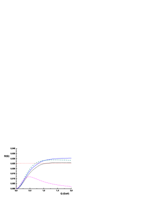
Figure 8: The Adler function from the N$\chi$QM contributions: dynamical quark loop (short dashed), quark + chiral loops + vector mesons (full line) versus the ALEPH data (dashed). The dash-dotted line is the prediction of the constituent quark model (ENJL) and the dotted line is the asymptotic freedom prediction, $1/4\pi^{2}$.

With the above set of parameters the Adler function in the vector channel calculated in N$\chi$QM (49) is presented in Fig. 8 and the model estimate for the hadronic vacuum polarization to $a_{\mu}$ given by (24) is

$$a_{\mu}^{\mathrm{hvp}~{}\left(1\right);\mathrm{N\chi QM}}=6.2\left(0.4\right)\cdot 10^{-8}\ ,$$ (56)

where the various contributions to $a_{\mu}^{\mathrm{hvp}~{}\left(1\right);\mathrm{N\chi QM}}$ are

$$a_{\mu}^{\mathrm{hvp}~{}\left(1\right);\mathrm{Qloop}}=5.3\cdot 10^{-8},\quad a_{\mu}^{\mathrm{hvp}~{}\left(1\right);\mathrm{Vmesons}}=0.1\cdot 10^{-8},\quad a_{\mu}^{\mathrm{hvp}~{}\left(1\right);\mathrm{\chi Loop}}=0.8\cdot 10^{-8}$$ (57)

and the error in (56) is due to incomplete knowledge of the higher order effects in nonchiral corrections. One may conclude, that the agreement of the N$\chi$QM estimate with the phenomenological determinations is rather good. With the same model parameters one gets the estimate for the $\alpha^{2}$ hadronic contribution to the $\tau$-lepton anomalous magnetic moments

$$a_{\tau}^{\mathrm{hvp}~{}\left(1\right);\mathrm{N\chi QM}}=3.1\left(0.2\right)\cdot 10^{-6}\ ,$$ (58)

which is in agreement with phenomenological determination

$$a_{\tau}^{\mathrm{hvp}~{}\left(1\right);\mathrm{exp}}=\left\{\begin{array}[c]{c}3.383\left(0.111\right)\cdot 10^{-6},\qquad\cite[cite]{[\@@bibref{}{Jegerlehner96}{}{}]},\\ 3.536\left(0.038\right)\cdot 10^{-6},\qquad\cite[cite]{[\@@bibref{}{Narison01}{}{}]}.\end{array}\right.\$$ (59)

7 Other model approaches to Adler function and $a_{\mu}^{\mathrm{hvp}~{}\left(1\right)}$.

In [33] the vector two-point function has been calculated in the extended Nambu–Jona-Lasinio (ENJL) model with the result

$$\Pi_{V}^{ENJL}(Q^{2})={\frac{\overline{\Pi}_{V}(Q^{2})}{1+Q^{2}{\frac{8\pi^{2}G_{V}}{3\Lambda_{r}^{2}}}\overline{\Pi}_{V}(Q^{2})}}\ ,$$ (60)

where $\overline{\Pi}_{V}(Q^{2})$ is given by a loop of constituent massive quarks as

$$\overline{\Pi}_{V}(Q^{2})=\frac{3}{2\pi^{2}}\int_{0}^{1}dxx\left(1-x\right)\Gamma\left(0,x_{Q}\right),$$ (61)

with $x_{Q}=\left(M_{Q}^{2}+Q^{2}x\left(1-x\right)\right)/\Lambda_{r}^{2}$ and $\Gamma\left(n,x\right)$ is the incomplete Gamma function. The parameters of the model are the constituent quark mass $M_{Q}=265$ MeV and the ultraviolet regulator of the model $\Lambda_{r}=1.165$ GeV. The Adler function predicted by ENJL model is presented in Fig. 8. It is clear from the figure that the ENJL model with constituent quarks does not interpolate correctly the transition from low to high momenta and fails to describe the hadronic data starting already at low momenta.Within ENJL the estimate of $a_{\mu}^{\mathrm{hvp}~{}\left(1\right)}$ was found as [34]

$$\left[a_{\mu}^{\mathrm{hvp}~{}\left(1\right)}\right]_{\mathrm{ENJL}}\simeq 7.5\cdot 10^{-8}\ .$$ (62)

Attempt to improve the situation has been done in [9] by introducing into the model infinite set of higher dimension terms. Effectively this procedure reduce to delocalization of the quark-quark interaction, the property inherent to the instanton-like models. Improved version of the ENJL is close to the predictions of the minimal hadronic approximation model (MHA) [9] based on the local duality. Assuming that the spectral density $\rho_{V}(t)$ is given by a sum ansatz of a single, zero width vector meson resonance and the QCD perturbative continuum contribution one has

$$\frac{1}{4\pi^{2}}\rho_{V}^{MHA}\left(t\right)=2f_{V}^{2}M_{V}^{2}\delta\left(t-M_{V}^{2}\right)+\frac{N_{c}}{12\pi^{2}}\theta\left(t-s_{0}\right),\qquad$$ (63)

and the Adler function in the Euclidean region is given by

$$A_{V}^{MHA}\left(Q^{2}\right)=2f_{V}^{2}M_{V}^{2}\frac{Q^{2}}{\left(Q^{2}+M_{V}^{2}\right)^{2}}+\frac{N_{c}}{12\pi^{2}}\frac{Q^{2}}{Q^{2}+s_{0}},$$ (64)

with $s_{0}\approx 1\div 1.5$ GeV² being the continuum threshold. This model predicts correct asymptotic behaviour of the Adler function. By taking the model parameters $M_{V}=0.750~{}GeV,$ $f_{V}^{2}=2f_{\pi}^{2}M_{V}^{2},$ $s_{0}\approx 1.35\quad\mathrm{GeV}$ one finds an estimate for $a_{\mu}^{\mathrm{hvp}~{}\left(1\right)}$ as [35]

$$\left[a_{\mu}^{\mathrm{hvp}~{}\left(1\right)}\right]_{\mathrm{MHA}}=\left(5.7\pm 1.7\right)\cdot 10^{-8}\ .$$ (65)

We also wish to recall that some time ago the hadronic contribution to the photon vacuum polarization to $a_{\mu}^{\mathrm{hvp}~{}\left(1\right)}$ has been estimated in the gauged nonlocal constituent quark model (GNC), the approach which is quite similar to the present model, with the result [25]

$$\left[a_{\mu}^{\mathrm{hvp}~{}\left(1\right)}\right]_{\mathrm{GNC}}=\left(6.3\pm 0.5\right)\cdot 10^{-8}\ .$$ (66)

It was also found that the model with momentum dependent quark mass give more favorable results with respect to the constituent quark model with constant masses. The GNC result is a sum of the dynamical quark loop contribution and of the one- and two-meson loops contributions. We think, however, that the two-loop contribution found in [25], which is almost the same as the one-loop result, is overestimated in the model calculations. As we already noted above the two-loop results have very narrow region of applicability.

Good agreement with the vector Adler function extracted from the experiment has been reached in [36] by using the analytic perturbative (AP) approach [37]. Within this model the perturbative expansion of the Adler function valid at high energy analytically continued to the infrared region where regular behaviour is predicted. There are two parameters in this model: the QCD parameter $\Lambda_{QCD}=420$ MeV and the light quark masses $m_{u,d}=250$ MeV. Note, that like to N$\chi$QM considerations the AP approach prefers to use rather low values of the quark masses to describe quantitatively the Adler function.

Finally we note that first evaluations of $a_{\mu}^{\mathrm{hvp}~{}}$ on the lattice appeared recently [38]

$$\left[a_{\mu}^{\mathrm{hvp}~{}}\right]_{\mathrm{Lattice}}=\left(4.46\pm 0.23\right)\cdot 10^{-8}.$$ (67)

Still this calculations contains rather big uncertainties and the above error does not take into account large systematical errors from the quenching approximation, unphysically large quark masses and finite volume effects.

8 $V-A$ correlator

For consistency we also give the expressions for the difference of the $V$ and $A$ correlators (37) in the extended N$\chi$QM and discuss the related chiral sum rules. The axial currents correlator is given by the sum of the dynamical quark loop, the intermediate axial-vector mesons propagators and the meson chiral loops (see some details in Appendix C). The dynamical quark loop contribution to the $V-A$ correlator has been found earlier in [8] and reads

$$\Pi_{V-A}^{\mathrm{Loop}}\left(Q^{2}\right) =-\frac{4N_{c}}{Q^{2}}\int\frac{d^{4}k}{\left(2\pi\right)^{4}}\frac{1}{D_{+}D_{-}}\left\{M_{+}M_{-}+\frac{4}{3}k_{\perp}^{2}\left[-\sqrt{M_{+}M_{-}}M^{\left(1\right)}\left(k_{+},k_{-}\right)+\right.\right.$$ (68)

$$\left.\left.+\left(\sqrt{M}^{\left(1\right)}\left(k_{+},k_{-}\right)\right)^{2}\left(\sqrt{M_{+}}k_{+}+\sqrt{M_{-}}k_{-}\right)^{2}\right]\right\}.$$

The integrand of the above expression is positive-definite in accordance with the Witten inequality.

In the extended model one gets the corrections from the vector and axial-vector intermediate mesons generated via the quark-quark rescattering to the $V-A$ polarization function

$$\Pi_{V-A}^{\mathrm{meson}}\left(Q^{2}\right)=\Pi_{V}^{\mathrm{meson}}\left(Q^{2}\right)-\Pi_{A}^{\mathrm{meson}}\left(Q^{2}\right),$$ (69)

where $\Pi_{V}^{\mathrm{meson}}\left(Q^{2}\right)$ is defined in (43) and the axial-vector polarization function due to the $a_{1}$-meson is

$$\Pi_{A}^{\mathrm{meson}}\left(Q^{2}\right)=-\frac{1}{2}\frac{G_{A}B_{A}^{2}\left(Q^{2}\right)}{1-G_{A}J_{A}^{T}\left(Q^{2}\right)},$$ (70)

where $B_{A}\left(q^{2}\right)$ is the transition form factor of the axial-vector current to quark-antiquark pair

$$B_{A}\left(Q^{2}\right) =8N_{c}i\int\frac{d^{4}k}{\left(2\pi\right)^{4}}\frac{f_{+}^{V}f_{-}^{V}}{D_{+}D_{-}}\left\{-M_{+}M_{-}-k_{+}k_{-}+\frac{2}{3}k_{\perp}^{2}\left[1-M^{(1)}\left(k_{+},k_{-}\right)\left(\sqrt{M_{+}}-\sqrt{M_{-}}\right)^{2}\right]-\right.$$ (71)

$$\left.-\frac{4}{3}k_{\perp}^{2}\frac{f_{-}f^{(1)}(k_{-},k_{+})}{D_{-}}\right\},$$

and $J_{A}^{T}\left(Q^{2}\right)$ is defined in (32). At zero momentum $B_{A}\left(0\right)\neq 0$ in accordance with the effect of $\pi-a_{1}$ meson mixing effect. As a consequence the total $V-A$ correlator is consistent with the first Weinberg sum rule: $\lim_{Q^{2}\rightarrow 0}Q^{2}\Pi_{V-A}^{T}\left(Q^{2}\right)=-f_{\pi}^{2}$, where $f_{\pi}^{2}$ is defined in (52). Due to very small value of $G_{A}$ the effect of the $a_{1}$ meson on the axial-vector correlator is very tiny.

Let us now consider the low-energy region where the effective model (26) should be fully predictive. From (68) and the Das-Guralnik-Mathur-Low-Yuong (DGMLY) sum rule [39], $\left(\Delta m_{\pi}^{2}\equiv m_{\pi^{\pm}}^{2}-m_{\pi^{0}}^{2}\right)$

$$-\frac{1}{4\pi^{2}}\int_{0}^{s_{0}\rightarrow\infty}dss\ln\frac{s}{\mu^{2}}\left[\rho_{V}\left(s\right)-\rho_{A}\left(s\right)\right]=\int_{0}^{\infty}dQ^{2}\left[-Q^{2}\Pi_{V-A}^{T}\left(Q^{2}\right)\right]=\frac{4\pi f_{\pi}^{2}}{3\alpha}\Delta m_{\pi}^{2},$$ (72)

we estimate the electromagnetic pion mass difference to be $\left(\Delta m_{\pi}\equiv m_{\pi^{\pm}}-m_{\pi^{0}}\right)$

$$\left[\Delta m_{\pi}\right]_{N\chi QM}=4.2\mathrm{~{}MeV},$$ (73)

which is in remarkable agreement with the experimental value (after subtracting the $m_{d}-m_{u}$ effect) [40]

$$\left[\Delta m_{\pi}\right]_{\mathrm{exp}}=4.43\pm 0.03\mathrm{~{}MeV}.$$ (74)

The $\pi^{+}-\pi^{0}$ electromagnetic mass difference is another observable which offers the possibility to test the quality of the matching between long-distance and short-distance behaviours.

With help of the Das-Mathur-Okubo (DMO) sum rule [41],

$$I_{\mathrm{DMO}}\left(s_{0}\rightarrow\infty\right)=\frac{1}{4\pi^{2}}\int_{0}^{s_{0}\rightarrow\infty}\frac{ds}{s}\left[\rho_{V}\left(s\right)-\rho_{A}\left(s\right)\right]=\left.\frac{\partial}{\partial Q^{2}}\left[Q^{2}\Pi_{V-A}^{T}\left(Q^{2}\right)\right]\right|_{Q^{2}\rightarrow 0}=\frac{1}{3}f_{\pi}^{2}\left\langle r_{\pi}^{2}\right\rangle-F_{A},$$ (75)

where $F_{A}$ is the pion axial-vector form factor and $\left\langle r_{\pi}^{2}\right\rangle$ is the electromagnetic pion radius squared, we estimate the electric polarizability of the charged pions by using [42]

$$\alpha_{\pi^{\pm}}^{E}=\frac{\alpha}{m_{\pi}}\left[\frac{\left\langle r_{\pi}^{2}\right\rangle}{3}-\frac{I_{\mathrm{DMO}}}{f_{\pi}^{2}}\right].$$ (76)

With the experimental value for the pion mean squared radius $\left\langle r_{\pi}^{2}\right\rangle=\left(0.439\pm 0.008\right)$ fm² [44] and the value of the $I_{DMO}$ integral estimated from the OPAL data [3]

$$\left[I_{\mathrm{DMO}}\left(s_{0}=m_{\tau}^{2}\right)\right]_{\mathrm{exp}}=\left(26.3\pm 1.8\right)\cdot 10^{-3}$$ (77)

one gets from Eq. (76) the result [3]

$$\left[\alpha_{\pi^{\pm}}^{E}\right]_{\mathrm{exp}}^{\mathrm{OPAL}}=\left(2.71\pm 0.88\right)\cdot 10^{-4}\mathrm{~{}fm}^{3}.$$ (78)

Another experimental estimate of the pion polarizability follows from recent measurments by PIBETA collaboration [45] of the pion axial-vector form factor $F_{A}$ with a result $F_{A}=0.443(15)\cdot F_{V}$ (full data set) and $F_{A}=0.480(16)\cdot F_{V}$ (kinematically restricted data set). Then using the Terentyev relation [47]

$$\alpha_{\pi^{\pm}}^{E}=\frac{\alpha F_{A}}{8\pi^{2}m_{\pi}f_{\pi}^{2}}.$$ (79)

one yields [46]

$$\left[\alpha_{\pi^{\pm}}^{E}\right]_{\mathrm{exp}}^{\mathrm{PIBETA}}=\left\{\begin{array}[c]{l}2.68(9)\cdot 10^{-4}\mathrm{~{}fm}^{3}\qquad\mathrm{{full\ data\ set},}\\ 2.90(9)\cdot 10^{-4}\mathrm{~{}fm}^{3}\qquad\mathrm{kinematically\ restricted\ data\ set}.\end{array}\right.$$ (80)

Within N$\chi$QM one obtains the estimates of the low energy constants

$$\left[I_{\mathrm{DMO}}\right]_{\mathrm{N\chi QM}}=23\cdot 10^{-3},\qquad\left[\left\langle r_{\pi}^{2}\right\rangle\right]_{\mathrm{N\chi QM}}=0.435\mathrm{~{}fm}^{2},$$ (81)

where these values are derived by calculating the derivatives of $\Pi^{V-A}\left(Q^{2}\right)$ and the electromagnetic pion form factor at zero momentum, with vector meson [28] and chiral loop corrections being included (see Appendix). By using the values given in Eqs. (81) we find from (76) the value

$$\left[\alpha_{\pi^{\pm}}^{E}\right]_{N\chi QM}=2.9\cdot 10^{-4}\mathrm{fm}^{3},$$ (82)

which is close to experimental numbers (78) and (80). Thus, we see that the model prediction for the pion polarizability, Eq. (82), is in a very reasonable agreement with the experimental data.

Next, we compare the $V-A$ correlator predicted in N$\chi$QM with the ALEPH data. As above, we use $s_{0}=2.5$ GeV² as an upper integration limit, the value at which all chiral sum rules are satisfied assuming that $\rho_{V-A}(s)=0$ at $s\geq s_{0}$, (13). Finally, a kinematic pole at $q^{2}=0$ is added to the axial-vector spectral function. The resulting unsubtracted dispersion relation between the measured spectral densities and the correlation functions becomes

$$\Pi_{V-A}^{T}\left(Q^{2}\right)=\frac{1}{4\pi^{2}}\int_{0}^{s_{0}}ds\frac{\rho_{V}\left(s\right)-\rho_{A}\left(s\right)}{s+Q^{2}}-\frac{f_{\pi}^{2}}{Q^{2}},$$ (83)

where $f_{\pi}^{2}$ is given by the first Weinberg sum rule

$$f_{\pi}^{2}=\frac{1}{4\pi^{2}}\int_{0}^{s_{0}}ds\left[v_{1}(s)-a_{1}(s)\right].$$ (84)

Having transformed the data into the Euclidean space, we may now proceed with the comparison to the model, which obviously applies to the Euclidean domain only. The resulting normalized $V-A$ correlation functions corresponding to the experimental data and the N$\chi$QM prediction are shown in Fig. 9.

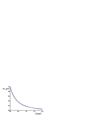
Figure 9: Normalized $V-A$ correlation function constructed in the N$\chi$QM (solid line) and reconstructed from the ALEPH experimental spectral function (dashed line).

9 Conclusions

In this work we have analyzed the vector Adler function for Euclidean (spacelike) momenta within an effective nonlocal chiral quark model motivated by the instanton model of QCD vacuum. To this end, we have derived the conserved vector and axial-vector currents and have constructed the Euclidean-momentum correlation functions of the vector and axial-vector currents in the extended by inclusion of vector mesons degrees of freedom model. The dominant contributions to the polarization functions and to the corresponding Adler functions come from the loop contributions of the light dynamical quarks. It is this contribution that provides the matching between low energy hadronized phase and the high energy QCD which is clearly seen in the behaviour of the Adler function (Figs. 2 and 8). The results obtained are close to estimates of the vector Adler function and the $V-A$ correlator extracted directly from the ALEPH data on hadronic inclusive $\tau$ decays and transformed by dispersion relations to the spacelike region.

We further use the vector Adler function to calculate the $\alpha^{2}$ hadronic contribution to the muon anomalous magnetic moment, $a_{\mu}^{\mathrm{hvp}~{}\left(1\right)}$, and found the value which is in reasonable agreement with the latest precise phenomenological numbers. The main reason why we discuss the N$\chi$QM is that it offers the possibility to go beyond the leading $O(p^{6})$ contribution of $\chi$PT. This will appear to be a crucial issue in consideration of the hadronic light-by-light contribution. Reproducing the phenomenological determination of $a_{\mu}^{\mathrm{hvp}~{}\left(1\right)}$, it becomes possible to make in future reliable estimates of $a_{\mu}^{\mathrm{hvp}~{}\left(2\right)}$ and $a_{\mu}^{\mathrm{h.~{}L\times L}}.$

In the N$\chi$QM extended by inclusion of vector and axial-vector mesons we show that the influence of these states on the Adler function and some low-energy observables is very small, at the level of few percents. This is because the physical states corresponding to these channels are rather heavy and, as consequence, have the couplings of quark-quark interactions much smaller than in the (pseudo-)scalar channels.

We also estimated the contributions to the correlators and the low energy observables of the nonchiral corrections, formally suppressed in $1/N_{c}$ expansion, by using the one loop results of the chiral perturbative theory. These corrections are typically of order $10-20\%$ comparing to the dynamical quark contributions. In this way the form factor dependence of the currents with mesons is not taken into account and predictions become untrustable at higher momenta. In perspective we plan to cure this disease and also take into account effectively the perturbative gluon corrections which become important at higher momenta.

From the properties of the $V-A$ correlator we have shown the fulfillment of the low-energy relations. The values of the $\pi^{\pm}-\pi^{0}$ electromagnetic mass difference and the electric pion polarizability are estimated and found to be close to the experimental values. We stress that the momentum dependence of the dynamical quark mass is crucial for the reproducing the empirical Adler function. The $V-A$ combination receives no contribution from perturbative effects and provides a clean probe for chiral symmetry breaking and a test ground for model verification.

Finally, we would like to note that the effective models based on the underlying symmetries of strong interactions are usually operative at low energies and fails in description of the high and even intermediate energy regions. An essential advantage of the nonlocal models is that they provide correct interpolation between the high energy behaviour where they are reduced to asymptotically free model and the low energy behaviour where they share the chiral symmetry and its spontaneous breaking. This is because the main elements of diagram technics, the quark propagator and the quark couplings with currents, become local at high virtualities. This property allows us to straightforwardly reproduce the leading terms of the operator product expansion. For instance, the correct high energy asymptotics are derived for the $V-A$ correlator (second Weinberg sum rule) [22, 8], the Adler function (this work), the topological susceptibility [8], the pion transition form factor [23] and some other quantities [50], while in all these cases the constituent quark model, with massive momentum independent quark masses, fails to explain the asymptotics. The nonlocality originated from the quark-quark interactions due to exchange of instantons also is of great importance in describing the hadronic distribution functions in order to produce the correct end-point behavior as it was shown for the case of the pion distribution amplitude [51] and structure function [50].

The author is grateful to W. Broniowski, S. B. Gerasimov, N. I. Kochelev, P. Kroll, S.V. Mikhailov, A. E. Radzhabov, O.P. Solovtsova and M. K. Volkov for useful discussions on the subject of the present work. AED thanks for partial support from RFBR (Grants nos. 02-02-16194, 03-02-17291, 04-02-16445), INTAS (Grant no. 00-00-366). We are grateful to the Heisenberg - Landau program for support.

Appendix A Conserved vector and axial-vector currents

The Noether currents and the corresponding vertices are formally obtained as functional derivatives of the action (26) with respect to the external fields at zero value of the fields. For our purpose, it is necessary to construct the quark-current vertices that involve one or two currents (contact terms). In the presence of the nonlocal interaction the conserved currents include both local and nonlocal terms. The technique of expansion of the path-ordered exponent in the external fields and derivation of the conserved currents has been reviewed in [18, 8]. Here we present the extension of the previuos results for the model (26) that includes in addition the vector and axial-vector mesons degrees of freedom.

The (axial-)vector meson contribution to the bare (axial-)vector vertex obtained by the differentiation the action (26) with respect to the external (axial-)vector field is given by the formula

$$\Delta\widetilde{\Gamma}_{\mu}^{(5)a}(p,q,p^{\prime}=p+q)=T^{a}\left\{-G_{J}f^{V}(p^{\prime})f^{V}(p)\left[\left(g_{\mu\nu}-\frac{q^{\mu}q^{\nu}}{q^{2}}\right)\gamma_{\nu}\widetilde{B}\left(q^{2}\right)+\frac{q^{\mu}\widehat{q}}{q^{2}}\widetilde{C}\left(q^{2}\right)\right]\right\}\left(\gamma_{5}\right),$$ (85)

where $q$ is the momentum corresponding to the current, and $p$ $(p^{\prime})$ is the incoming (outgoing) momentum of the quark,

$$\widetilde{B}\left(q^{2}\right) =16N_{c}i\int\frac{d^{4}k}{\left(2\pi\right)^{4}}\frac{2}{3}k_{\perp}^{2}\frac{f^{V}\left(k\right)f^{V(1)}(k,k+q)}{D\left(k\right)},$$ (86)

$$\widetilde{C}\left(q^{2}\right) =16N_{c}i\int\frac{d^{4}k}{\left(2\pi\right)^{4}}\left(kq\right)\frac{f^{V}\left(k\right)f^{V}(k+q)}{D\left(k\right)}.$$ (87)

In order to obtain the full vertex corresponding to the conserved (axial-)vector current it is necessary to add the term which contains the (axial-)vector meson propagator. The addition of this term to the full conserved vertex acquires the form

$$\Delta\Gamma_{\mu}^{\left(5\right)a}(p,q,p^{\prime}=p+q)=T^{a}\left[-\left(g_{\mu\nu}-\frac{q^{\mu}q^{\nu}}{q^{2}}\right)\gamma_{\nu}\frac{G_{J}B_{J}\left(q^{2}\right)}{1-G_{J}J_{J}^{T}\left(q^{2}\right)}f^{V}\left(p\right)f^{V}\left(p^{\prime}\right)\right]\left(\gamma_{5}\right),$$ (88)

where the factors $B_{J}\left(q^{2}\right)$ define the virtual transition of the meson to the (axial-)vector current and are given above in (44) and (71).

Appendix B Vector and axial-vector mesons properties

To fit the parameters of the extended model (54) and (55), we consider the main decay modes of (axial-) vector mesons. The quark-meson couplings are fixed by the $\rho,$ $\omega$ and $a_{1}$ masses from the condition (35) and equal to

$$g_{\rho q}=0.61,\quad g_{\omega q}=0.59,\quad g_{a_{1}q}=0.08.$$ (89)

The decay $\rho\rightarrow\pi\pi$ is described by the amplitude

$$\left\langle\pi^{a}(p_{1})\pi^{b}(p_{2})\left|\rho^{c}(P)\right.\right\rangle=i\varepsilon^{abc}g_{\rho\pi\pi}\left(p_{2}-p_{1}\right)_{\mu}\epsilon^{\mu},$$ (90)

where $p_{i}$ are momenta of pions, $\epsilon^{\mu}$ is the $\rho$-meson polarization vector. With parameters given in Sect. 6 we obtain $g_{\rho\pi\pi}=6.1$ and the decay width $\Gamma_{\rho\pi\pi}=154$ MeV which reasonably well agrees with the experimental value $\left[\Gamma_{\rho\pi\pi}\right]_{\mathrm{exp}}=149.2\pm 0.7$ MeV [44].

The decays of vector mesons to $e^{+}e^{-}$ pair and the transition of the $a_{1}$ meson to the axial-vector current are described by the amplitudes

$$\left\langle 0\left|J^{\mu a}\right|\rho_{s}^{b}\right\rangle=-g_{\rho\gamma}\delta^{ab}\epsilon_{s}^{\mu},\quad\left\langle 0\left|J^{\mu}\right|\omega_{s}\right\rangle=-g_{\omega\gamma}\delta^{ab}\epsilon_{s}^{\mu},\quad\left\langle 0\left|J^{\mu 5}\right|a_{1s}^{b}\right\rangle=-g_{a_{1}}\delta^{ab}\epsilon_{s}^{\mu}.$$ (91)

We have obtained the values for the photon-vector meson couplings $g_{\rho\gamma}=0.114$ GeV${}^{2},\quad g_{\omega\gamma}=0.039$ GeV² and the axial coupling $g_{a_{1}}=0.082$ GeV² which have to be compared with the empirical values $g_{\rho\gamma}^{\exp}=0.1177\quad$GeV${}^{2},$ $g_{\omega\gamma}^{\exp}=0.0359$ GeV² [44].

Appendix C Non-chiral corrections

Here we give the expressions for nonchiral corrections. Hadronic spectral functions for the processes $\rho\rightarrow\pi\pi\rightarrow\rho$ and $a_{1}\rightarrow\sigma\pi\rightarrow a_{1}$ are given by general expression:

$$\frac{1}{t}\frac{1}{\pi}\operatorname{Im}\Pi\left(t\right)=\frac{1}{3\cdot 16\pi^{2}}\sqrt{\left(1-\frac{m_{1}^{2}+m_{2}^{2}}{t}\right)^{2}-2\frac{m_{1}^{2}+m_{2}^{2}}{t^{2}}}\left[\left(1-\frac{m_{1}^{2}+m_{2}^{2}}{t}\right)^{2}-\frac{4m_{1}^{2}m_{2}^{2}}{t^{2}}\right]\Theta\left(t-\left(m_{1}+m_{2}\right)^{2}\right),$$ (92)

where $m_{1,2}$ are meson masses in the intermediate state. One has $m_{1}=m_{2}=m_{\pi}$ for the first process and $m_{1}=m_{\pi},m_{2}=m_{\sigma}$ for the second one. The contribution of chiral loops to the vector polarization function reads as

$$\Pi_{\chi\mathrm{Loop}}^{V}\left(Q^{2}\right)=\frac{1}{48\pi^{2}}\left[p\left(\frac{Q^{2}}{4m_{\pi}^{2}}\right)+p\left(\frac{Q^{2}}{4m_{K}^{2}}\right)\right],$$ (93)

where

$$p\left(z\right)=-\left[\frac{2}{3}\frac{3+4z}{z}+\left(\frac{z+1}{z}\right)^{3/2}\left(\operatorname{arctanh}\left[\frac{1+2z}{2\sqrt{z\left(z+1\right)}}\right]+i\frac{\pi}{2}\right)\right].$$

The leading order corrections to the low energy constants and to the electromagnetic pion mass difference are correspondingly [48, 49]

$$\left[I_{\mathrm{DMO}}\right]_{\mathrm{\chi-loops}}=-\frac{1}{48\pi^{2}}\ln\frac{m_{\pi}^{2}}{m_{\sigma}^{2}},\qquad\left[\left\langle r_{\pi}^{2}\right\rangle\right]_{\mathrm{\chi-loops}}=\frac{3}{f_{\pi}^{2}}\left[I_{\mathrm{DMO}}\right]_{\mathrm{\chi-loops}},\qquad\left[\Delta m_{\pi}^{2}\right]_{\mathrm{\chi-loops}}=-\frac{3\alpha}{4\pi}m_{\pi}^{2}\ln\frac{m_{\pi}^{2}}{m_{\sigma}^{2}},$$ (94)

with chiral logarithm being approximately

$$\ln\frac{m_{\pi}^{2}}{m_{\sigma}^{2}}\approx-3.$$ (95)

Above estimate corresponds to the $\sigma-$pole position in $\pi\pi$ $S$-wave isoscalar scattering around $600$ MeV. In Table 2 we present separately different terms contributing to the physical constants.

Table 2.

	quark loop	intermed. mesons	chiral loop	total	exp
$\Delta m_{\pi}\left(\mathrm{MeV}\right)$	$3.95$	$0.13$	$0.36$	$4.44$	$4.43$
$I_{\mathrm{DMO}}\cdot 10^{3}$	$16.72$	$0.008$	$6.16$	$22.89$	$26.30$
$\left\langle r_{\pi}^{2}\right\rangle\left(\mathrm{fm}^{2}\right)$	$0.334$	$0.013$	$0.087$	$0.435$	$0.439$

References

• [1] See for review, e.g., T. Schafer, E.V. Shuryak, Rev. Mod. Phys. 70 (1998) 323.
• [2] R. Barate et.al. [ALEPH Collaboration], Eur. Phys. J. C 4 (1998) 409.
• [3] K. Ackerstaff et.al. [OPAL Collaboration], Eur. Phys. J. C 7 (1999) 471.
• [4] G.W. Bennett et al. [Muon g-2 Collaboration], Phys. Rev. Lett. 89 (2002) 101804 [Erratum-ibid. 89 (2002) 129903]; H. N. Brown et al. [Muon g-2 Collaboration], Phys. Rev. Lett. 86 (2001) 2227; G.W. Bennett et al. [Muon g-2 Collaboration], arXiv:hep-ex/0401008.
• [5] S.G. Gorishnii, A.L. Kataev, S.A.Larin, Phys. Lett. B 259 (1991) 144; L.R. Surguladze, M.A. Samuel, Phys. Rev. Lett. 66 (1991) 560 [Erratum-ibid. 66 (1991) 2416].
• [6] K.G. Chetyrkin, Phys. Lett. B 391 (1997) 402.
• [7] K.G. Chetyrkin, S. Narison, V.I. Zakharov, Nucl. Phys. B 550 (1999) 353.
• [8] A. E. Dorokhov, W. Broniowski, Eur. Phys. J. C 32 (2003) 79.
• [9] S. Peris, M. Perrottet, E. de Rafael, JHEP 9805 (1998) 011.
• [10] M. Davier, S. Eidelman, A. Hocker and Z. Zhang, Eur. Phys. J. C 31 (2003) 503.
• [11] S. Ghozzi, F. Jegerlehner, Phys. Lett. B 583 (2004) 222.
• [12] T. Kinoshita, M. Nio, arXiv:hep-ph/0402206.
• [13] A. Czarnecki, W. J. Marciano and A. Vainshtein, Phys. Rev. D 67 (2003) 073006.
• [14] J.F. de Troconiz, F.J. Yndurain, arXiv:hep-ph/0402285.
• [15] B. Krause, Phys. Lett. B 390 (1997) 392.
• [16] M. Knecht, A. Nyffeler, Phys. Rev. D 65 (2002) 073034.
• [17] K. Melnikov, A. Vainshtein, hep-ph/0312226.
• [18] I. V. Anikin, A. E. Dorokhov and L. Tomio, Phys. Part. Nucl. 31 (2000) 509 [Fiz. Elem. Chast. Atom. Yadra 31 (2000) 1023].
• [19] B.E. Lautrup and E. de Rafael, Nuovo Cimento, 64 A, (1969), 322.
• [20] S.V. Mikhailov, A.V. Radyushkin, Sov. J. Nucl. Phys. 49 (1989) 494 [Yad. Fiz. 49 (1988) 794]; S. V. Mikhailov and A. V. Radyushkin, Phys. Rev. D 45 (1992) 1754.
• [21] A. E. Dorokhov, S. V. Esaibegian and S. V. Mikhailov, Phys. Rev. D 56 (1997) 4062; A. E. Dorokhov, S. V. Esaibegian, A. E. Maximov and S. V. Mikhailov, Eur. Phys. J. C 13 (2000) 331.
• [22] W. Broniowski, Mesons in non-local chiralq uark models, in Hadron Physics: Effective theories of low-energy QCD, Coimbra, Portugal, September 1999, AIP Conference Proceedings 508 (1999) 380, eds. A. H. Blin and B. Hiller and M. C. Ruivo and C. A. Sousa and E. van Beveren, AIP, Melville, New York, hep-ph/9911204.
• [23] A. E. Dorokhov, JETP Letters, 77 (2003) 63 [Pisma ZHETF, 77 (2003) 68]; I. V. Anikin, A. E. Dorokhov and L. Tomio, Phys. Lett. B 475 (2000) 361.
• [24] E. Golowich, J. Kambor, Nucl. Phys. B 447 (1995) 373.
• [25] B. Holdom, R. Lewis and R.R. Mendel, Z. Phys. C 63 (1994) 71.
• [26] A.E. Dorokhov, S.V. Esaibegyan, A. E. Maximov, S.V. Mikhailov, Eur. Phys. J. C 13 (2000) 331.
• [27] A. E. Dorokhov and W. Broniowski, Phys. Rev. D 65 (2002) 094007.
• [28] A.E. Dorokhov, A.E. Radzhabov, M.K. Volkov, arXiv:hep-ph/0311359.
• [29] J. Gasser, H. Leutwyler, Annals Phys. 158, (1984) 142.
• [30] K. Yamawaki, V.I. Zakharov, arXiv:hep-ph/9406399.
• [31] F. Jegerlehner, Nucl. Phys. Proc. Suppl. 51C (1996) 131.
• [32] S.Narison, Phys. Lett. B 513 (2001) 53[Erratum-ibid. B 526 (2002) 414]
• [33] J. Bijnens, E. de Rafael, H. Zheng, Z. Phys. C 62 (1994) 437.
• [34] E. de Rafael, Phys. Lett. B 322 (1994) 239.
• [35] M. Knecht, arXiv:hep-ph/0307239.
• [36] K.A. Milton, I.L. Solovtsov, O.P. Solovtsova, Phys. Rev. D 64 (2001) 016005.
• [37] D.V. Shirkov and I.L. Solovtsov, Phys. Rev. Lett. 79 (1997) 1209.
• [38] T. Blum, Phys. Rev. Lett. 91 (2003) 052001; M. Gockeler et.al. [QCDSF Collaboration], arXiv:hep-lat/0312032.
• [39] T. Das, G.S. Guralnik, V.S. Mathur, F.E. Low, J.E. Young, Phys. Rev. Lett. 18 (1967) 759.
• [40] J. Gasser and H. Leutwyler, Nucl. Phys. B 250 (1985) 465.
• [41] T. Das, V.S. Mathur, S. Okubo, Phys. Rev. Lett. 18 (1967) 761.
• [42] S.B. Gerasimov, JINR-E2-11693, 1978; Yad. Fiz. 29 (1979) 513 [Sov. J. Nucl. Phys. 29, 259 (1979)] [Erratum, 32, 156 (1980)].
• [43] A.E. Dorokhov, M.K. Volkov, J. Hufner, S.P. Klevansky, P. Rehberg, Z. Phys. C 75 (1997) 127.
• [44] K. Hagiwara et al. [Particle Data Group Collaboration], Phys. Rev. D 66 (2002) 010001.
• [45] E. Frlez et al., arXiv:hep-ex/0312029.
• [46] D. Počanić, private communication, (2004).
• [47] M.V. Terentev, Yad. Fiz. 16 (1972) 162 [Sov. J. Nucl. Phys., 16 (1972) 87].
• [48] H.J. Hippe, S.P. Klevansky, Phys. Rev. C 52 (1995) 2172.
• [49] S.P. Klevansky, R.H. Lemmer, C.A.Wilmot, Phys. Lett. B 457 (1999) 1.
• [50] A. E. Dorokhov and L. Tomio, Phys. Rev. D 62 (2000) 014016; I.V. Anikin, A.E. Dorokhov, A.E. Maksimov, L. Tomio, V. Vento, Nucl. Phys. A 678 (2000) 175.
• [51] A.E. Dorokhov, Nuovo Cim. A 109 (1996) 391.