NOVEL OPPORTUNITIES FOR EW BREAKING
FROM LOW-SCALE SUSY BREAKING

In supersymmetric scenarios with a low scale of SUSY breaking [$\sqrt{F}=O(TeV)$] the conventional MSSM Higgs sector can be substantially modified, mainly because the Higgs potential contains additional effective quartic terms. The Higgs spectrum can be dramatically changed, and the lightest state can be much heavier than in usual SUSY scenarios. Novel opportunities for electroweak breaking arise, and the electroweak scale may be obtained in a less fine-tuned way for wide ranges of $\tan\beta$ and the Higgs mass, offering a possible solution to the MSSM fine-tuning problem.

1 Low-scale SUSY breaking

The simplest effective description of SUSY breaking (SUSY) assumes that the theory contains a SUSYsector not coupled directly to the observable sector, but rather through a heavier ”messenger” sector (characterized by a mass scale $M$) coupled to both. Let us parameterize the SUSYsector simply by a singlet chiral field $T$, whose $F$-term takes a non zero vacuum expectation value (vev) thereby breaking SUSY. After integrating out the heavy physics associated to the messenger sector, the low-energy theory for the observable fields $\varphi$ will contain non-renormalizable couplings between $T$ and $\varphi$. These operators give rise to soft terms (such as scalar soft masses), but also hard terms (such as quartic scalar couplings):

$$\int d^{4}\theta{1\over M^{2}}|T|^{2}|\varphi|^{2}\Rightarrow m_{\rm soft}^{2}\sim{F^{2}\over M^{2}}\ ;\;\;\;\;\int d^{4}\theta{1\over M^{4}}|T|^{2}|\varphi|^{4}\Rightarrow\lambda_{\makebox[24.18501pt][l]{$\line(4,1){19.0}$ {\tiny{SUSY}}}}\sim{F^{2}\over M^{4}}\sim{m_{\rm soft}^{2}\over M^{2}}\ .$$ (1)

Phenomenology requires $m_{\rm soft}={\cal O}(1\,{\rm TeV})$, but this leaves undetermined the scale $\sqrt{F}$ of SUSY. We can consider two extreme possibilities: 1) In models with SUSYmediated by gravity $M\sim 10^{18}$ GeV implies $\sqrt{F}\sim 10^{11}$ GeV. In such cases the large hierarchy $M\gg\sqrt{F}\gg m_{\rm soft}$ makes unobservable the $\lambda_{\makebox[24.18501pt][l]{$\line(4,1){19.0}$ {\tiny{SUSY}}}}$ contributions. 2) If $M$ is not far from the TeV scale, then $\sqrt{F}$ would be of the same order. We are interested in such low-scale SUSYscenarios$\!{}^{{\bf?},{\bf?},{\bf?},{\bf?}}$, in particular to explore the implications of the hard terms in eq. (1) for electroweak symmetry breaking.

In ref.$\!{}^{{\bf?}}$ we performed a model independent analysis of such effects using this effective theory approach. The Higgs potential of the resulting low-energy effective theory is a generic two Higgs doublet model (THDM). In terms of the invariants ${\cal I}_{1}=|H_{1}|^{2}$, ${\cal I}_{2}=|H_{2}|^{2}$, ${\cal I}_{12}=H_{1}\cdot H_{2}$:

$$V = m_{1}^{2}{\cal I}_{1}+m_{2}^{2}{\cal I}_{2}+(m_{3}^{2}{\cal I}_{12}+{\mathrm{h}.c.})$$ (2)

$$+ {1\over 2}\lambda_{1}{\cal I}_{1}^{2}+{1\over 2}\lambda_{2}{\cal I}_{2}^{2}+\lambda_{3}{\cal I}_{1}{\cal I}_{2}+\lambda_{4}|{\cal I}_{12}|^{2}+\left[{1\over 2}\lambda_{5}{\cal I}_{12}^{2}+(\lambda_{6}{\cal I}_{1}+\lambda_{7}{\cal I}_{2}){\cal I}_{12}+{\mathrm{h}.c.}\right]\ ,$$

with $T$-dependent coefficients. (If the $T$ field is heavy enough it can be integrated out.) The SUSYcontributions to the Higgs quartic couplings are no longer negligible and can be easily larger than the ordinary MSSM values, given by gauge couplings, and this has a deep impact on the pattern of EW breaking. Some of the main differences with respect to the MSSM are the following$\!{}^{{\bf?}}$. a) There is no need of radiative corrections to trigger EW breaking. It occurs already at tree-level (which is just fine since the effects of RG running are small for a low cut-off scale $M$). b) EW breaking occurs naturally only in the Higgs sector, as desired. c) The parameter space that gives a proper EW breaking is larger (the constraints from unbounded from below directions can be absent). d) The Higgs spectrum and properties can be very different due to very different quartic couplings. In particular, the MSSM upper bound on the mass of the lightest Higgs field no longer applies. In fact, all Higgses might be significantly heavier than the $Z^{0}$. e) There is an extra degree of freedom in the scalar sector, coming from the complex singlet $T$. f) The Higgs quartic couplings $\lambda_{5},\lambda_{6},\lambda_{7}$ can be complex and introduce new possible sources of $CP$ violation already at tree level. g) As we will see, the changes of the Higgs potential allow for a drastic reduction of the fine tuning required for the EW breaking.

2 A concrete model

Let us now present a concrete example$\!{}^{{\bf?}}$. The superpotential is given by (with the notation introduced above, plus ${\cal T}=|T|^{2}$)

$$W=\Lambda_{S}^{2}T+\mu{\cal I}_{12}+{\ell\over 2M}{\cal I}_{12}^{2}\ ,$$ (3)

and the Kähler potential is

$$K={\cal T}+{\cal I}_{1}+{\cal I}_{2}-{\alpha_{t}\over 4M^{2}}{\cal T}^{2}+{\alpha_{1}\over M^{2}}{\cal T}({\cal I}_{1}+{\cal I}_{2})+{e_{1}\over 2M^{2}}\left({\cal I}_{1}^{2}+{\cal I}_{2}^{2}\right)\ .$$ (4)

(All parameters are real with $\alpha_{t}>0$.) Here $\Lambda_{S}$ is the SUSYscale and $M$ the ‘messenger’ scale (see previous section). The typical soft masses are $\sim\tilde{m}\equiv\Lambda_{S}^{2}/M$. In particular, the mass of the scalar component of $T$ is ${\cal{O}}(\tilde{m})$ and, after integrating this field out, the effective potential for $H_{1}$ and $H_{2}$ is a 2HDM with very particular Higgs mass terms: $m_{1}^{2}=m_{2}^{2}=\mu^{2}-\alpha_{1}\tilde{m}^{2}$, $m_{3}^{2}=0$ and Higgs quartic couplings like those of the MSSM plus contributions of order $\mu/M$ and $\tilde{m}^{2}/M^{2}$:

$$\lambda_{1}=\lambda_{2} = {1\over 4}(g^{2}+g_{Y}^{2})+2\alpha_{1}^{2}{\tilde{m}^{2}\over M^{2}}\ ,$$

$$\lambda_{3} = {1\over 4}(g^{2}-g_{Y}^{2})+{2\over M^{2}}(\alpha_{1}^{2}\tilde{m}^{2}-e_{1}\mu^{2})\ ,$$

$$\lambda_{4} = -{1\over 2}g^{2}-2\left(e_{1}+2{\alpha_{1}^{2}\over\alpha_{t}}\right){\mu^{2}\over M^{2}}\ ,$$

$$\lambda_{5} = 0\ ,$$

$$\lambda_{6}=\lambda_{7} = {\ell\mu\over M}\ .$$ (5)

The explicit expressions for the spectrum of Higgs masses can be found in $\!{}^{{\bf?}}$. Here we plot the masses as a function of the superpotential parameter $\ell$ in fig. 1, together with $\tan\beta\equiv\langle H_{2}\rangle/\langle H_{1}\rangle$, which is 1 if $\ell$ is below some critical value. The differences with the MSSM are apparent.

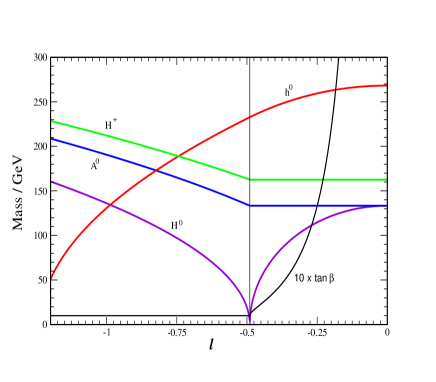
Figure 1: Higgs spectrum of the example model as a function of $\ell$. Also shown is $\tan\beta$ (scaled by a factor 10).

3 The fine tuning problem of the MSSM

The MSSM Higgs sector is a very constrained THDM. The potential $V^{\rm MSSM}$ is of the form (2) with $m_{1,2}^{2}=\mu^{2}+m_{H_{1,2}}^{2}$ and $m_{3}^{2}=B\mu$, where $m_{H_{i}}^{2}$ and $B$ are soft masses and $\mu$ is the Higgs mass term in the superpotential, $W\supset\mu H_{1}\cdot H_{2}$. The quartic Higgs couplings are simply

$$V_{4}^{\rm MSSM}=\frac{1}{8}(g^{2}+g_{Y}^{2})(|H^{0}_{1}|^{2}-|H^{0}_{2}|^{2})^{2}\ .$$ (6)

Minimization of $V^{\rm MSSM}$ leads to a vev $v^{2}\equiv 2(\langle H^{0}_{1}\rangle^{2}+\langle H^{0}_{2}\rangle^{2})$ and thus to a mass for the $Z^{0}$ gauge boson, $M_{Z}^{2}=\frac{1}{4}(g^{2}+g_{Y}^{2})v^{2}$.

The size of $v$ is determined by the parameters of $V^{\rm MSSM}$, in particular $m_{i}^{2}$, which depend on the initial parameters, $p_{\alpha}$ [for the MSSM these are the soft scalar masses $m$, the $\mu-$parameter, the gaugino masses $M$ and the trilinear soft terms $A$ at the initial (high energy) scale]. Therefore, $v^{2}=v^{2}(p_{1},p_{2},\cdots)$. As an example, for the case of large $\tan\beta$ and taking the initial scale to be $M_{GUT}$ one gets

$$M_{Z}^{2}\simeq-2.02\mu_{0}^{2}+3.57M_{0}^{2}+0.07m_{0}^{2}+0.22A_{0}^{2}+0.75A_{0}M_{0}\ ,$$ (7)

where the subindex $0$ indicates values evaluated at $M_{GUT}$ and we have assumed universality. Getting the right value for $M_{Z}$ (or $v$) in a natural way requires that the $p_{\alpha}$’s are not too large, which in turn requires that the masses of superpartners should be $\stackrel{{\scriptstyle<}}{{{}_{\sim}}}$ few hundred GeV. Actually, the available experimental data already imply that the ordinary MSSM is significantly fine tuned$\!{}^{{\bf?},{\bf?},{\bf?},{\bf?},{\bf?},{\bf?}}$. Consider for instance the lower bound on the lightest Higgs boson mass

$$m_{h}^{2}\leq M_{Z}^{2}\cos^{2}2\beta+{3m_{t}^{4}\over 2\pi^{2}v^{2}}\log{M_{\rm SUSY}^{2}\over m_{t}^{2}}+...$$ (8)

where $m_{t}$ is the (running) top mass ($\simeq 171$ GeV for $M_{t}=178$ GeV). Since the experimental lower bound, $(m_{h})_{\rm exp}\geq 115$ GeV, exceeds the tree-level contribution, the radiative corrections must be responsible for the difference, and this translates into a lower bound on $M_{\rm SUSY}$:

$$M_{\rm SUSY}\;\stackrel{{\scriptstyle>}}{{{}_{\sim}}}\;e^{-2.1\cos^{2}2\beta}e^{\left({m_{h}}/{62\ {\rm GeV}}\right)^{2}}m_{t}\;\stackrel{{\scriptstyle>}}{{{}_{\sim}}}\;3.8\ m_{t}\ ,$$ (9)

where the last figure corresponds to $m_{h}=115$ GeV and large $\tan\beta$, which is the most favorable case for the fine tuning. The last equation implies sizeable soft terms, $\tilde{m}\stackrel{{\scriptstyle>}}{{{}_{\sim}}}2m_{t}$, which in turn translates into large fine-tunings.

We adopt as a measure of the fine tuning associated to $p_{\alpha}$ the quantity $\Delta_{p_{\alpha}}$ defined by $\!{}^{{\bf?}}$

$${\delta v^{2}\over v^{2}}=\Delta_{p_{\alpha}}{\delta p_{\alpha}\over p_{\alpha}}\ ,$$ (10)

where $\delta v^{2}$ is the change induced in $v^{2}$ by a change $\delta p_{\alpha}$ in $p_{\alpha}$. Absence of fine tuning requires that $\Delta_{p_{\alpha}}$ should not be larger than ${\cal O}(10)$.

The fine-tuning problem of the MSSM is illustrated by fig. (2) which has $\tilde{m}=M_{0}=m_{0}=A_{0}$. It shows how the fine-tuning $\Delta_{\mu^{2}}$ grows with increasing $\tilde{m}$ and decreasing $\tan\beta$. Insisting in $\Delta_{\mu^{2}}<10$ would require $m_{h}<105$ GeV and $\tilde{m}<175$ GeV. It also shows that for soft masses $\tilde{m}^{2}\sim av^{2}$ the fine-tuning scales like $\Delta_{\mu^{2}}\sim 20a$. That is, the MSSM fine-tuning is much larger than one would naively expect ($\Delta_{\mu^{2}}\sim a$).

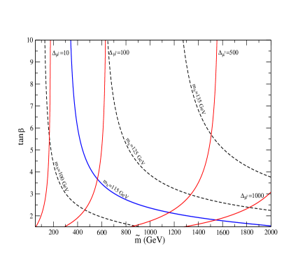
Figure 2: Fine tuning in the MSSM (measured by $\Delta_{\mu^{2}}$, solid lines) in the $(\tilde{m},\tan\beta)$ plane. Dashed lines are contour lines of constant Higgs mass.

Why is this so? There are three main reasons [1) to 3) below]. To better understand them let us write the Higgs potential along the breaking direction in the $H_{1}^{0},H_{2}^{0}$ space. It is of SM-like form:

$$V={1\over 2}m^{2}v^{2}+{1\over 4}\lambda v^{4}\ ,$$ (11)

where $\lambda$ and $m^{2}$ are functions of the $p_{\alpha}$ parameters and $\tan\beta$, in particular $m^{2}=c_{\beta}^{2}\,m_{1}^{2}(p_{\alpha})+s_{\beta}^{2}\,m_{2}^{2}(p_{\alpha})-s_{2\beta}\,m_{3}^{2}(p_{\alpha})$. Minimization of (11) leads to

$$v^{2}={-m^{2}\over\lambda}\ .$$ (12)

1) In the MSSM $\lambda$ turns out to be quite small:

$$\lambda_{\rm MSSM}={1\over 8}(g^{2}+g_{Y}^{2})\cos^{2}2\beta\ \simeq\ {1\over 15}\cos^{2}2\beta\ .$$ (13)

This has the effect of amplifying whatever cancellations are taking place inside $m^{2}$ in (12). This implies a fine tuning $\stackrel{{\scriptstyle>}}{{{}_{\sim}}}15$ times larger than expected from naive dimensional considerations. The previous $\lambda_{\rm MSSM}$ was evaluated at tree-level but radiative corrections make $\lambda$ larger, thus reducing the fine tuning$\!{}^{{\bf?},{\bf?}}$. Since $m_{h}^{2}\sim 2\lambda v^{2}$, the ratio $\lambda_{\rm tree}/\lambda_{\rm 1-loop}$ is basically the ratio $(m_{h}^{2})_{\rm tree}/(m_{h}^{2})_{\rm 1-loop}$, so for large $\tan\beta$ the previous factor 15 is reduced by a factor $M_{Z}^{2}/m_{h}^{2}$.

2) Although for a given size of the soft terms the radiative corrections reduce the fine tuning, sizeable radiative corrections require large soft terms, which in turn worsens the fine tuning. A given increase in $\tilde{m}^{2}$ reflects linearly in $m^{2}$ but only logarithmically in $\lambda$, so the fine tuning usually gets worse. In fact, the Higgs bound (8) implies that radiative corrections should be sizeable and therefore this restricts the allowed parameter space to regions of large fine tuning.

3) Thanks to supersymmetry, $m^{2}$ is not sensitive to large quadratic corrections in the MSSM but it receives sizeable logaritmic corrections $\delta m^{2}\propto(\tilde{m}^{2}/16\pi^{2})\log(M_{GUT}^{2}/\tilde{m}^{2})$, which can be interpreted as the effect of the RG running of $m^{2}$ from $M_{GUT}$ down to the electroweak scale. Typically, the large logarithms and the numerical factors compensate the one-loop factor, so that the corrections are quite large. This is the origin of the large coefficients that appear in formulae such as (7) which also have an impact on the value of the fine-tuning.

4 Fine tuning in models with low-scale SUSY breaking

It is remarkable that low-scale SUSYmodels of the type discussed in the first two sections have all the necessary ingredients to ameliorate the shortcomes of the MSSM regarding the fine-tuning of EW breaking. Let us see this following the same numbering as above:

1) As explained in Sect. 1, tree-level quartic Higgs couplings larger than in the MSSM are natural in scenarios in which the breaking of SUSY occurs at a low-scale$\!{}^{{\bf?},{\bf?},{\bf?},{\bf?}}$ (not far from the TeV scale).

2) If the quartic Higgs couplings are already large at tree level, the LEP Higgs mass bound can be evaded without the need of large radiative corrections, and therefore regions of parameter space with lower soft masses are not excluded and in them the fine-tuning is naturally smaller.

3) In models with a low SUSY breaking scale RG effects are expected to play no significant role since the cut-off scale is much closer to the electroweak scale.

All these three improvements can cooperate to make EW breaking much more natural than in the MSSM. We show this in fig. (3) for the model of Sect. 2. The reader should keep in mind that this model was not constructed with the goal of reducing fine-tuning in mind. The corresponding expression for $\Delta_{\mu^{2}}$, as evaluated from eq.(10), is

$$\Delta_{\mu^{2}}=-{\mu^{2}\over\lambda v^{2}}\left[1+v^{2}\left({ls_{2\beta}\over 2\mu M}-{1\over M^{2}}(e_{1}+{\alpha_{1}^{2}\over\alpha_{t}})s_{2\beta}^{2}\right)\right]\ .$$ (14)

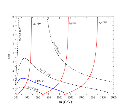
Figure 3: Fine tuning in the $(\tilde{m},\tan\beta)$ plane in the low-scale SUSY breaking scenario of Sect. 2. Dashed lines are contour lines of constant $m_{h}$. The LEP bound is also shown.

In fig. 3 we see an overall decrease in the size of fine-tuning of one order of magnitude with respect to the MSSM. Also, restricting the fine tuning to be less than 10 does not impose an upper bound on the Higgs masses, in contrast with the MSSM case. As a result, the LEP bounds do not imply a large fine tuning. In any case, for $\Delta_{\mu^{2}}\leq 10$ we do find an upper bound $\tilde{m}\stackrel{{\scriptstyle<}}{{{}_{\sim}}}500$ GeV, so that LHC would either find superpartners or revive an (LHC) fine tuning problem for these scenarios (although the problem would be much softer than in the MSSM).

I would like to thank Andrea Brignole, Alberto Casas, Irene Hidalgo and Ignacio Navarro for a most enjoyable collaboration. This work is supported in part by the Spanish Ministry of Science and Technology through a MCYT project (FPA2001-1806).

References

References

- [1] J. A. Casas, J. R. Espinosa and I. Hidalgo, JHEP 0401 (2004) 008 [hep-ph/0310137].
- [2] R. Barbieri and G. F. Giudice, Nucl. Phys. B 306 (1988) 63.
- [3] B. de Carlos and J. A. Casas,, Phys. Lett. B 309 (1993) 320 [hep-ph/9303291].
- [4] M. Olechowski and S. Pokorski, Nucl. Phys. B 404 (1993) 590.
- [5] G. W. Anderson and D. J. Castaño, Phys. Lett. B 347 (1995) 300.
- [6] P. Ciafaloni and A. Strumia, Nucl. Phys. B 494 (1997) 41 [hep-ph/9611204].
- [7] P. H. Chankowski, J. R. Ellis and S. Pokorski, Phys. Lett. B 423 (1998) 327 [hep-ph/9712234]; R. Barbieri and A. Strumia, Phys. Lett. B 433 (1998) 63 [hep-ph/9801353]; P. H. Chankowski, J. R. Ellis, M. Olechowski and S. Pokorski, Nucl. Phys. B 544 (1999) 39 [hep-ph/9808275]; G. L. Kane and S. F. King, Phys. Lett. B 451 (1999) 113 [hep-ph/9810374]; M. Bastero-Gil, G. L. Kane and S. F. King, Phys. Lett. B 474 (2000) 103 [hep-ph/9910506].
- [8] K. Harada and N. Sakai, Prog. Theor. Phys. 67 (1982) 1877;
- [9] A. Brignole, F. Feruglio and F. Zwirner, Nucl. Phys. B 501 (1997) 332 [hep-ph/9703286].
- [10] N. Polonsky and S. Su, Phys. Lett. B 508 (2001) 103 [hep-ph/0010113]; Phys. Rev. D 63 (2001) 035007 [hep-ph/0006174].
- [11] A. Brignole, J. A. Casas, J. R. Espinosa and I. Navarro, [hep-ph/0301121].
- [12] A. Strumia, Phys. Lett. B 466 (1999) 107 [hep-ph/9906266].
- [13] See e.g. D. Comelli and C. Verzegnassi, Phys. Lett. B 303 (1993) 277; J. R. Espinosa and M. Quirós, Phys. Lett. B 302 (1993) 51 [hep-ph/9212305]; M. Cvetič, D. A. Demir, J. R. Espinosa, L. L. Everett and P. Langacker, Phys. Rev. D 56 (1997) 2861 [Erratum-ibid. D 58 (1998) 119905] [hep-ph/9703317]; P. Batra, A. Delgado, D. E. Kaplan and T. M. Tait, [hep-ph/0309149].
- [14] M. Drees, Int. J. Mod. Phys. A 4 (1989) 3635; J. R. Ellis, J. F. Gunion, H. E. Haber, L. Roszkowski and F. Zwirner, Phys. Rev. D 39 (1989) 844; P. Binetruy and C. A. Savoy, Phys. Lett. B 277 (1992) 453. J. R. Espinosa and M. Quirós, Phys. Lett. B 279 (1992) 92; Phys. Rev. Lett. 81 (1998) 516 [hep-ph/9804235]; G. L. Kane, C. F. Kolda and J. D. Wells, Phys. Rev. Lett. 70 (1993) 2686 [hep-ph/9210242].
- [15] M. Bastero-Gil, C. Hugonie, S. F. King, D. P. Roy and S. Vempati, Phys. Lett. B 489 (2000) 359 [hep-ph/0006198].