DECAYS OF SUPERNOVA RELIC NEUTRINOS

We propose that future observation of supernova relic neutrino (SRN) can be used to probe neutrino decay models. We focus on invisible (e.g., Majoron) decays, and work out the general solution of SRN kinetic equations in the presence of oscillations plus decay. We then apply the general solution to specific decay scenario, and show that the predicted SRN event rate can span the whole range below the current experimental bound. Therefore, future SRN observations will surely have an impact on the neutrino decay parameter space.

1 Introduction

In general, massive neutrinos can not only mix, but also decay. The most stringent and safe limit comes from the nonobservation of decay effects on solar $\nu$ flux. However, due to the relatively small distance from the Sun, this limit is very weak, namely $\tau_{i}/m_{i}\gtrsim 5\times 10^{-4}\mathrm{\ s/eV}$, where $\tau_{i}$ represents the lifetime of the eigenstates $\nu_{i}$ with mass $m_{i}$. Therefore, the possibility of neutrino decay with longer lifetimes (and coming from other astrophysical sources) cannot be excluded.

Here we focus on the diffuse $\nu$ background produced by all past core-collapse Supernovae (SN) in the Universe—the so-called supernova relic neutrinos (SRN). Future observations of SRN can probe decay lifetimes of cosmological interest. In fact, for SRN decay effects to be observable in our universe, it must be roughly $\tau_{i}E/m_{i}\lesssim 1/H_{0}$, where $H_{0}$ is the Hubble constant. By setting $H_{0}=70\;\mathrm{km}\,\mathrm{s}^{-1}\,\mathrm{Mpc}^{-1}$ and taking $E\sim O(10)$ MeV (i.e., in the energy range probed by supernova neutrinos), a rough upper bound for the “SRN neutrino decay observability” is obtained, namely ${\tau_{i}}/{m_{i}}\lesssim O(10^{11})\mathrm{\ s/eV}$. The comparison of this bound with the previous solar limit implies that SRN leave many decades in $\tau_{i}/m_{i}$ open to experimental and theoretical investigations.

Motivated by this challenging opportunity, in this talk we aim at showing how to incorporate the effects of both flavor transitions and decays in observable SRN spectra, by solving the SRN kinetic equations for two-body non-radiative $\nu$ decay. This work is based on the results obtained in $\!{}^{{\bf?}}$, to which we refer the interested reader for further details.

The plan of the talk is as follows. In Sec. 2 we discuss the general case of $3\nu$ flavor transitions followed by decays, and give the explicit solution of the neutrino kinetic equations for generic decay parameters. Specific numerical examples (inspired by neutrino-Majoron decay models) are given in Sec. 3, in order to show representative SRN event rates and energy spectra in the presence of decay. Finally, in Sec. 4 we draw the conclusion of our work.

2 Three-neutrino flavor transitions and decays

In this Section we discuss and solve the neutrino kinetic equations in the general case of 3$\nu$ flavor transitions plus decay. Notice that, for $\tau_{i}/m_{i}$ values above the solar $\nu$ bound, SRN flavor transitions occur in matter (and become incoherent) well before neutrino decay losses become significant, so that hypothetical interference effects between the two phenomena can be neglected. For our purposes, flavor transitions inside the supernova can thus be taken as decoupled from the subsequent (incoherent) propagation and decay of mass eigenstates in vacuum.

2.1 3$\nu$ flavor transitions

We assume the active 3$\nu$ oscillation scenario. In this framework, the 3$\nu$ squared mass spectrum can be cast in the form $(m^{2}_{1},m^{2}_{2},m^{2}_{3})=M^{2}+\left(-\frac{\delta m^{2}}{2},+\frac{\delta m^{2}}{2},\pm\Delta m^{2}\right)$, where $M^{2}$ fixes the absolute $\nu$ mass scale; $\delta m^{2}$ and $\Delta m^{2}$ govern two independent $\nu$ oscillation frequencies, with $|\Delta m^{2}|\gg\delta m^{2}$, as indicated by current data. The case of $+\Delta m^{2}$ ($-\Delta m^{2}$) characterizes the so-called normal (inverted) hierarchy. The elements of the mixing matrix $U$ are parametrized in terms of three mixing angles $(\theta_{12},\theta_{13},\theta_{23})$.

The yield  $Y_{\nu_{i}}$ of the $i$-th mass eigenstate at the surface of the supernova can be calculated by taking into account the stellar matter effects on $\nu$ propagation in SN. These effects are parametrized in term of a level crossing probability $P_{H}=P_{H}(\Delta m^{2},\theta_{13})$ among the instantaneous eigenstates of the Hamiltonian (the so called “matter eigenstates”) in the dense medium  . The final results for the yields $Y_{\nu_{i}}$ at the exit from the supernova are collected in Table I in $\!{}^{{\bf?}}$.

2.2 3$\nu$ decays

At the exit of SN, $\nu_{i}$ mass eigenstates evolve indipendently until they reach the surface of the Earth. However, in their propagation in vacuum, they may decay. The number density of mass eigenstates $n_{\nu_{i}}(E,z)$ per unit of comoving volume and of energy at redshift $z$ can be obtained through a direct integration of the neutrino kinetic equations, as described below.

For ultrarelativistic relic neutrinos $\nu_{i}$ the kinetic equations take the form

$$\left[\frac{\partial}{\partial t}-H(t)E\frac{\partial}{\partial E}-H(t)\right]n_{\nu_{i}}(E,t)=R_{\mathrm{SN}}(t)Y_{\nu_{i}}(E)+\sum_{m_{j}>m_{i}}q_{ji}(E,t)-\Gamma_{i}\,\frac{m_{i}}{E}\,n_{\nu_{i}}(E,t)\ .$$ (1)

The left-hand side (l.h.s.) of Eq. (1) represents the Liouville operator for ultra-relativistic $\nu$, where $H(t)$ is the Hubble constant at the time $t$. The right-hand side (r.h.s.) of Eq. (1) contains two source terms and one sink term. The first source term quantifies the standard (decay-independent) emission of $\nu_{i}$ from core-collapse supernovae, which depends on the supernova formation rate $R_{SN}(t)$. The second source term, in which

$$q_{ji}(E,t)=\int_{E}^{\infty}dE^{\prime}n_{\nu_{j}}(E^{\prime},t)\,B(\nu_{j}\to\nu_{i})\Gamma_{j}\,\frac{m_{j}}{E^{\prime}}\,\psi_{\nu_{j}\to\nu_{i}}(E^{\prime},E)\ ,$$ (2)

quantifies the population increase of $\nu_{i}$ due to decays from heavier states $\nu_{j}$, with decay width $\Gamma_{j}=1/\tau_{j}$, branching ratio $B(\nu_{j}\to\nu_{i})$ and normalized decay energy spectrum $\psi_{\nu_{j}\to\nu_{i}}$. The last (sink) term on the r.h.s. of Eq. (1) represents the loss of $\nu_{i}$ due to decay to lighter states with width $\Gamma_{i}$.

Our result is that these equations can be directly integrated, by rewriting them in terms of the redshift variable $z=z(t)$ and of a rescaled energy parameter $\varepsilon=\varepsilon(E,z)$. By replacing back the variable $E=\varepsilon(1+z)$, one obtains the general solution of the neutrino kinetic equations,

$$n_{\nu_{i}}(E,z) = \frac{1}{1+z}\int_{z}^{\infty}\frac{dz^{\prime}}{H(z^{\prime})}\,\left[R_{\mathrm{SN}}(z^{\prime})\,Y_{\nu_{i}}\left(E\frac{1+z^{\prime}}{1+z}\right)\right.$$ (3)

$$+\left.\sum_{m_{j}>m_{i}}q_{ji}\left(E\frac{1+z^{\prime}}{1+z},z^{\prime}\right)\right]e^{-m_{i}\Gamma_{i}[\xi(z^{\prime})-\xi(z)](1+z)/E}\ ,$$

where we have introduced the auxiliary function

$$\xi(z)=\int_{0}^{z}dz^{\prime}\,H^{-1}(z^{\prime})(1+z^{\prime})^{-2}\ .$$ (4)

In practice, these equations can be integrated numerically by following the decay sequence, i.e., starting from the heaviest state ($q_{ji}=0$) and ending at the lightest state ($\Gamma_{i}=0$).

Finally, the $\bar{\nu}_{e}$ flux at Earth (redshift $z=0$), relevant for the inverse $\beta$ decay reaction $\bar{\nu}_{e}+p\to n+e^{+}$ in a Cherenkov detector, is given by

$$n_{\bar{\nu}_{e}}(E)\simeq\cos^{2}\theta_{12}\,n_{\bar{\nu}_{1}}(E,0)+\sin^{2}\theta_{12}\,n_{\bar{\nu}_{2}}(E,0)\,.$$ (5)

3 Applications to scenario inspired by Majoron models

In this section we apply the general results of Sec. 2.2 to some representative decay scenarios, inspired by Majoron models. We consider only nonradiative (invisible) decays of the kind $\nu_{i}\to{\stackrel{{\scriptstyle{}_{(-)}}}{{\nu}}\!\!}_{j}+X$, where an heavier neutrino $\nu_{i}$ decays into a ligher detectable (anti)neutrino ${\stackrel{{\scriptstyle{}_{(-)}}}{{\nu}}\!\!}_{j}$ plus an invisible massless (pseudo)scalar particle $X$, i.e. a “Majoron”.

We examine and compare a few representative $3\nu$ decay cases, which provide SRN yields higher, comparable, or lower than for no decay. For simplicity, we focus on two phenomenologically interesting cases in which the branching ratios and decay spectra become model-independent, namely, the case of quasidegenerate (QD) neutrino masses ($m_{i}\simeq m_{j}\gg m_{i}-m_{j}$) and of strongly hierarchical (SH) neutrino masses ($m_{i}\gg m_{j}\simeq 0$). Table II in $\!{}^{{\bf?}}$ displays the relevant characteristics of the QD and SH cases.

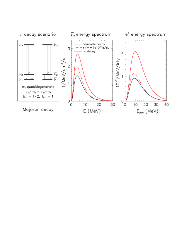
Figure 1: Supernova relic $\bar{\nu}_{e}$ spectrum (middle panel), and associated positron spectrum from $\bar{\nu}_{e}+p\to n+e^{+}$ (right panel), for a decay scenario with normal hierarchy and quasidegenerate masses (left panel, with $\tau/m$ and branching ratios assignments).

3.1 Three-family decays for normal hierarchy and quasidegenerate masses

This decay scenario provides SRN densities generally higher than for no decay. The relevant features of this scenario are graphically shown in the left panel of Figure 1. The QD approximation forbids decays of neutrinos into antineutrinos and vice versa (see Table II in $\!{}^{{\bf?}}$).

By construction, the decay scenario considered in this section is thus governed by just one free parameter ($\tau/m$). Notice that, for $\tau/m\sim O(10^{10})$ s/eV, SRN decay effects are expected to occur on a truly cosmological scale. For much larger values of $\tau/m$, the no-decay case is recovered. For much smaller values of $\tau/m$, SRN decay is instead complete, all SRN being in the lightest mass eigenstate $\bar{\nu}_{1}$ at the time of detection.

Figure 1 shows the supernova relic $\bar{\nu}_{e}$ energy spectrum, and the associated (observable) positron spectrum, for the considered decay scenario. The energy spectra for complete decay (red solid curves) appear to be a factor of $\sim 2$ higher than for no decay (black solid curve).

For incomplete neutrino decay (i.e., for $\tau/m\sim O(10^{10})$ s/eV), one expects an intermediate situation leading to a SRN flux moderately higher than for no decay. Figure 1 displays the results for a representative case ($\tau/m=7\times 10^{10}$ s/eV, red dotted curves). In conclusion, the decay scenario examined in this section can lead to an increase of the SRN rate, as compared with the case of no decay. The enhancement can be as large as a factor $\sim 2$, the larger the more complete is the decay.

3.2 Three-family decays for normal hierarchy and $m_{1}\simeq 0$

This decay scenario provides observable SRN densities generally comparable to the no-decay case. In this case, the approximation of strong hierarchy (SH) can be applied to the decays of $\nu_{2,3}$ (and of $\bar{\nu}_{2,3}$). Figure 2 shows the supernova relic $\bar{\nu}_{e}$ and positron spectra for this scenario where, as depicted in the left panel, all decay channels are open. This complex decay chain produces a substantial enhancement of the SRN energy spectrum at low energy, visible as a “pile-up” of decayed neutrinos with degraded energy in the middle panel of Fig. 2. Analogously, the case of incomplete decay (e.g., $\tau/m=7\times 10^{10}$ s/eV, green dotted curves), is appreciably different from the cases of no decay and of complete decay only at low energy.

In this scenario, the interesting effects of decay are almost completely confined to low $\bar{\nu}_{e}$ energies, and are thus washed out in the observable $e^{+}$ spectrum, due to the cross section enhancement of high-energy features. In conclusion, the $e^{+}$ spectra for the three cases of complete, incomplete, and no decay, turn out to be very similar to each other (right panel of Fig. 2), and so in this scanario decay effects cannot easily be distinguished through future SRN observations.

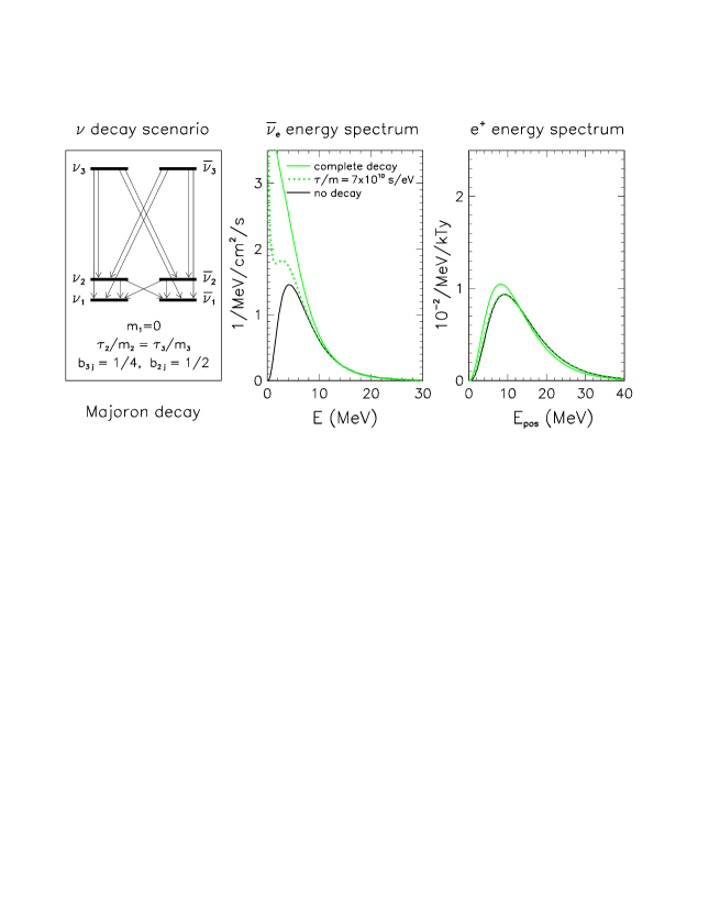
Figure 2: Supernova relic $\bar{\nu}_{e}$ spectrum (middle panel), and associated positron spectrum from $\bar{\nu}_{e}+p\to n+e^{+}$ (right panel), for a decay scenario with normal hierarchy and $m_{1}\simeq 0$ (left panel, with $\tau/m$ and branching ratios assignments).

3.3 Three-family decay for inverted hierarchy

We conclude our survey of $3\nu$ decays by discussing a scenario where the SRN density is generally suppressed, as compared with the case of no decay. The main features of this scenario are graphically shown in the left panel of Figure 3. It results that only the decay $\bar{\nu}_{2}\to\bar{\nu}_{1}$ (where the QD approximation is applicable) is relevant to SRN observations. In fact, decays to $\bar{\nu}_{3}$ provide a negligible amount of $\bar{\nu}_{e}$’s ($\propto\sin^{2}\theta_{13}\lesssim 10^{-2}$), so that the absolute value of $m_{3}$ makes no difference. In the above scenario, the case of complete decay ($\tau/m\ll O(10^{10})$ s/eV) is trivial: since the final state is populated only by $\bar{\nu}_{3}$ (and $\nu_{3}$), the relic density of $\bar{\nu}_{e}$ is negligibly small ($\propto\sin^{2}\theta_{13}$). The nontrivial case of incomplete decay ($\tau/m\sim O(10^{10})$ s/eV) is then expected to lead to an intermediate suppression of the SRN density. Figure 3 shows the numerical results for the specific value $\tau/m=7\times 10^{10}$ s/eV, in both cases $P_{H}=1$ (solid curves) and $P_{H}=0$ (dashed curves). The neutrino spectra for incomplete decay (blue curves) appear to be systematically lower than the corresponding no-decay spectra (black curves), although the difference is mitigated in the positron spectra (right panel of Fig. 3).

In conclusion, in the inverted hierarchy scenario of Fig. 3 the SRN signal is generally suppressed by neutrino decay, and can eventually disappear for complete decay.

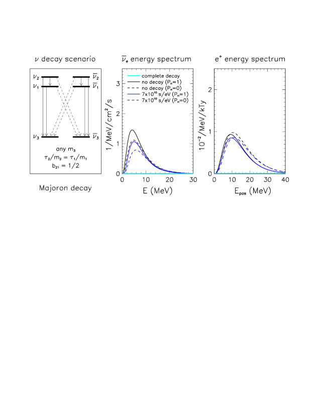
Figure 3: Supernova relic $\bar{\nu}_{e}$ spectrum (middle panel), and associated positron spectrum from $\bar{\nu}_{e}+p\to n+e^{+}$ (right panel), for a decay scenario with inverted hierarchy and generic $m_{3}$ (left panel, with $\tau/m$ and branching ratios assignments).

3.4 Overview and summary of $3\nu$ decay

We think it useful to show also the behavior of the SRN signal for continuous values of the free parameter $\tau/m$, for the three different decay scenario discussed above. Figure 4 shows the positron event rate integrated in the energy window $E_{e^{+}}\in[10\,,\,20]$ MeV which might become accessible to future, low-background SRN searches $\!{}^{{\bf?}}$. For each scenario, the rate is normalized to the standard expectations for no decay and normal hierarchy (NH), and is plotted as a function of $\tau/m$. It results that neutrino decay can enlarge the reference no-decay predictions for observable positron rates by any factor $f$ in the range $\sim[0\,,\,2.3]$, depending on the particular decay scenario and provided that $\tau/m$ is in the cosmologically interesting range below $O(10^{11})$ s/eV.

Since the current experimental upper bound on the SRN flux from SK is just a factor of $\sim 2$–3 above typical no-decay expectations $\!{}^{{\bf?}}$, future observations below such bound are likely to have an impact on neutrino decay models. If experimental and theoretical uncertainties can be kept smaller than a factor of two (a nontrivial task), one should eventually be able to rule out, at least, either the lowermost or the uppermost values in the range $f\in[0\,,\,2.3]$, i.e., one of the extreme cases of “complete decay.” Optimistically, one might then try to constrain specific decay models and lifetime-to-mass ratios through observations.

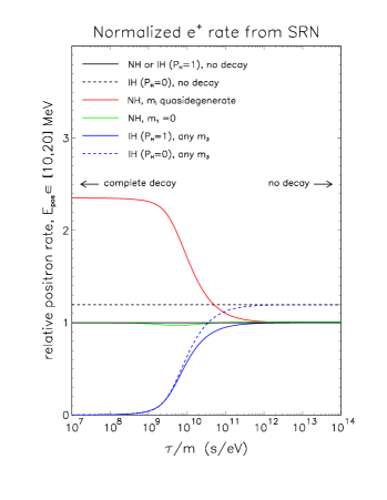
Figure 4: Positron event rates in the energy range $[10\,,\,20]$ MeV for various decay scenarios, normalized to standard expectations for normal hierarchy and no decay. Notice how the expectations branch out (and then reach the complete decay limit) in the cosmologically relevant range $\tau/m\lesssim 10^{11}$ s/eV.

4 Conclusion

Neutrino decays with cosmologically relevant neutrino lifetimes [$\tau_{i}/m_{i}\lesssim O(10^{11})$ s/eV] can, in principle, be probed through observations of supernova relic $\bar{\nu}_{e}$ (SRN). We have shown how to incorporate the effects of both flavor transitions and decays in the calculation of the SRN density, by finding the general solution of the neutrino kinetic equations for generic two-body nonradiative decays. We have then applied such solution to three representative decay scenarios which lead to an observable SRN density larger, comparable, or smaller than for no decay. In the presence of decay, the expected range of the SRN rate is significantly enlarged (from zero up to the current upper bound). Future SRN observations can thus be expected to constrain at least some extreme decay scenarios and, in general, to test the likelihood of specific decay models, as compared with the no-decay case.

References

References

- [1] G.L. Fogli, E. Lisi, A. Mirizzi and D. Montanino, hep-ph/0401227, to appear on Phys. Rev. D.
- [2] J.F. Beacom and M.R. Vagins, hep-ph/0309300, submitted to Phys. Rev. Lett.
- [3] Super-Kamiokande Collaboration, M. Malek et al., Phys. Rev. Lett. 90, 061101 (2003).