Waiting for precise measurements of $K^{+}\rightarrow\pi^{+}\nu\bar{\nu}$ and $K_{\rm L}\rightarrow\pi^{0}\nu\bar{\nu}$

Abstract

In view of future plans for accurate measurements of the theoretically clean branching ratios $Br(K^{+}\rightarrow\pi^{+}\nu\bar{\nu})$ and $Br(K_{\rm L}\rightarrow\pi^{0}\nu\bar{\nu})$, that should take place in the next decade, we collect the relevant formulae for quantities of interest and analyze their theoretical and parametric uncertainties. We point out that in addition to the angle $\beta$ in the unitarity triangle (UT) also the angle $\gamma$ can in principle be determined from these decays with respectable precision and emphasize in this context the importance of the recent NNLO QCD calculation of the charm contribution to $K^{+}\rightarrow\pi^{+}\nu\bar{\nu}$ and of the improved estimate of the long distance contribution by means of chiral perturbation theory. In addition to known expressions we present several new ones that should allow transparent tests of the Standard Model (SM) and of its extensions. While our presentation is centered around the SM, we also discuss models with minimal flavour violation and scenarios with new complex phases in decay amplitudes and meson mixing. We give a brief review of existing results within specific extensions of the SM, in particular the Littlest Higgs Model with T-parity, $Z^{\prime}$ models, the MSSM and a model with one universal extra dimension. We derive a new “golden” relation between $B$ and $K$ systems that involves $(\beta,\gamma)$ and $Br(K_{\rm L}\rightarrow\pi^{0}\nu\bar{\nu})$ and investigate the virtues of $(R_{t},\beta)$, $(R_{b},\gamma)$, $(\beta,\gamma)$ and $(\bar{\eta},\gamma)$ strategies for the UT in the context of $K\to\pi\nu\bar{\nu}$ decays with the goal of testing the SM and its extensions.

I Introduction

The rare decays of $K$ and $B$ mesons play an important role in the search for the underlying flavour dynamics and in particular in the search for the origin of CP violation Buras (2005a, 2003, b); Buchalla et al. (1996a); Buras (1998); Fleischer (2002, 2004); Ali (2003); Hurth (2003); Nir (2001); Buchalla (2003); Isidori et al. (2005). Among the many $K$ and $B$ decays, the rare decays $K^{+}\rightarrow\pi^{+}\nu\bar{\nu}$ and $K_{\rm L}\rightarrow\pi^{0}\nu\bar{\nu}$ are very special as their branching ratios can be computed to an exceptionally high degree of precision that is not matched by any other loop induced decay of mesons. In particular the theoretical uncertainties in the prominent decays like $B\to X_{s}\mu^{+}\mu^{-}$ and $B_{s}\to\mu^{+}\mu^{-}$ amount typically to $\pm 10\%$ or larger at the level of the branching ratio, although progress in the calculation of the branching ratio of $B\to X_{s}\gamma$ at the NNLO level shows that in this case an error below 10$\%$ is in principle possible Becher and Neubert (2007); Misiak et al. (2007). On the other hand the corresponding uncertainties in $K_{\rm L}\rightarrow\pi^{0}\nu\bar{\nu}$ amount to 1-2$\%$ Buchalla and Buras (1993b, a); Misiak and Urban (1999); Buchalla and Buras (1999). In the case of $K^{+}\rightarrow\pi^{+}\nu\bar{\nu}$, the presence of the internal charm contributions in the relevant $Z^{0}$ penguin and box diagrams contained the theoretical perturbative uncertainty of $\pm 7\%$ at the NLO level Buchalla and Buras (1999); Buchalla and Buras (1994a), but this uncertainty has been recently reduced down to $\pm 1-2\%$ through a complete NNLO calculation Buras et al. (2005b, 2006a).

The reason for the exceptional theoretical cleanness of $K^{+}\rightarrow\pi^{+}\nu\bar{\nu}$ and $K_{\rm L}\rightarrow\pi^{0}\nu\bar{\nu}$ Littenberg (1989) is the fact that the required hadronic matrix elements can be extracted, including isospin breaking corrections Marciano and Parsa (1996); Mescia and Smith (2007), from the leading semileptonic decay $K^{+}\to\pi^{0}e^{+}\nu$. Moreover, extensive studies of other long-distance contributions Rein and Sehgal (1989); Hagelin and Littenberg (1989); Lu and Wise (1994); Fajfer (1997); Geng et al. (1996); Ecker et al. (1988); Falk et al. (2001); Buchalla and Isidori (1998) and of higher order electroweak effects Buchalla and Buras (1998) have shown that they can safely be neglected in $K_{\rm L}\rightarrow\pi^{0}\nu\bar{\nu}$ and are small in $K^{+}\rightarrow\pi^{+}\nu\bar{\nu}$. In particular, the most recent improved calculation of long distance contributions to $K^{+}\rightarrow\pi^{+}\nu\bar{\nu}$ results in an enhancement of the relevant branching ratio by $6\pm 2\%$. Further progress in calculating these contributions is in principle possible with the help of lattice QCD Isidori et al. (2006a). Some recent reviews on $K\to\pi\nu\bar{\nu}$ can be found in Buras (2005a, 2003, b); Isidori (2003); Isidori et al. (2005).

We are fortunate that, while the decay $K^{+}\rightarrow\pi^{+}\nu\bar{\nu}$ is CP conserving and depends sensitively on the underlying flavour dynamics, its partner $K_{\rm L}\rightarrow\pi^{0}\nu\bar{\nu}$ is purely CP violating within the Standard Model (SM) and most of its extensions and consequently depends also on the mechanism of CP violation. Moreover, the combination of these two decays allows to eliminate the parametric uncertainties due to the CKM element $|V_{cb}|$ and $m_{t}$ in the determination of the angle $\beta$ in the unitarity triangle (UT) or equivalently of the phase of the CKM element $V_{td}$ Buchalla and Buras (1994b); Buchalla and Buras (1996). The resulting theoretical uncertainty in $\sin 2\beta$ is comparable to the one present in the mixing induced CP asymmetry $a_{\psi K_{S}}$ and with the measurements of both branching ratios at the $\pm 10\%$ and $\pm 5\%$ level, $\sin 2\beta$ could be determined with $\pm 0.08$ and $\pm 0.04$ precision, respectively. This independent determination of $\sin 2\beta$ with a very small theoretical error offers a powerful test of the SM and of its simplest extensions in which the flavour and CP violation are governed by the CKM matrix, the so-called MFV (minimal flavour violation) models Buras (2005a, 2003, b); Buras et al. (2001b); D’Ambrosio et al. (2002). Indeed, in $K\to\pi\nu\bar{\nu}$ the phase $\beta$ originates in $Z^{0}$ penguin diagrams ($\Delta S=1$), whereas in the case of $a_{\psi K_{S}}$ in the $B^{0}_{d}-\bar{B}^{0}_{d}$ box diagrams ($\Delta B=2$). Any “non-minimal” contributions to $Z^{0}$ penguin diagrams and/or box $B^{0}_{d}-\bar{B}^{0}_{d}$ diagrams would then be signaled by the violation of the MFV “golden” relation Buchalla and Buras (1994b)

$$(\sin 2\beta)_{\pi\nu\bar{\nu}}=(\sin 2\beta)_{\psi K_{S}}.$$ (I.1)

Now, strictly speaking, according to the common classification of different types of CP violation Buras (2005a, 2003, b); Fleischer (2002, 2004); Ali (2003); Hurth (2003); Nir (2001); Buchalla (2003), both the asymmetry $a_{\psi K_{S}}$ and a non-vanishing rate for $K_{\rm L}\rightarrow\pi^{0}\nu\bar{\nu}$ in the SM and in most of its extensions signal the CP violation in the interference of mixing and decay. However, as the CP violation in mixing (indirect CP violation) in $K$ decays is governed by the small parameter $\varepsilon_{K}$, one can show Littenberg (1989); Buchalla and Buras (1996); Grossman and Nir (1997) that the observation of $Br(K_{\rm L}\rightarrow\pi^{0}\nu\bar{\nu})$ at the level of $10^{-11}$ and higher is a manifestation of a large direct CP violation with the indirect one contributing less than $\sim 1\%$ to the branching ratio. The great potential of $K_{\rm L}\rightarrow\pi^{0}\nu\bar{\nu}$ in testing the physics beyond the SM has been summarized in Bryman et al. (2006).

Additionally, this large direct CP violation can be directly measured without essentially any hadronic uncertainties, due to the presence of the $\nu\bar{\nu}$ in the final state. This should be contrasted with the very popular studies of direct CP violation in non-leptonic two–body $B$ decays Buras (2005a, 2003, b); Fleischer (2002, 2004); Ali (2003); Hurth (2003); Nir (2001); Buchalla (2003), that are subject to significant hadronic uncertainties. In particular, the extraction of weak phases requires generally rather involved strategies using often certain assumptions about the strong dynamics Harrison and Quinn (1998); Ball et al. (2000); Anikeev et al. (2001). Only a handful of strategies, which we will briefly review in Section IX, allow direct determinations of weak phases from non-leptonic $B$ decays without practically any hadronic uncertainties.

Returning to (I.1), an important consequence of this relation is the following one Buras and Fleischer (2001): for a given $\sin 2\beta$ extracted from $a_{\psi K_{S}}$, the measurement of $Br(K^{+}\rightarrow\pi^{+}\nu\bar{\nu})$ determines up to a two-fold ambiguity the value of $Br(K_{\rm L}\rightarrow\pi^{0}\nu\bar{\nu})$, independent of any new parameters present in the MFV models. Consequently, measuring $Br(K_{\rm L}\rightarrow\pi^{0}\nu\bar{\nu})$ will either select one of the possible values or rule out all MFV models. Recent analyses of the MFV models indicate that one of these values is very unlikely Bobeth et al. (2005); Haisch and Weiler (2007). A spectacular violation of the relation (I.1) is found in the context of new physics scenarios with enhanced $Z^{0}$ penguins carrying a new CP-violating phase Buras et al. (2004b, a); Nir and Worah (1998); Buras et al. (1998); Colangelo and Isidori (1998); Buras and Silvestrini (1999); Buras et al. (2000); Buchalla et al. (2001); Atwood and Hiller (2003). An explicit realization of such a scenario is the Littlest Higgs Model with T-parity Blanke et al. (2007b) which we will discuss in Section VIII.

Another important virtue of $K^{+}\rightarrow\pi^{+}\nu\bar{\nu}$ is a theoretically clean determination of $|V_{td}|$ or equivalently of the length $R_{t}$ in the unitarity triangle. This determination is only subject to theoretical uncertainties in the charm sector, that amount after the recent NNLO calculation to $\pm 1-2\%$. The remaining parametric uncertainties in the determination of $|V_{td}|$ related to $|V_{cb}|$ and $m_{t}$ should be soon reduced to the 1-2$\%$ level. Finally, the decay $K_{\rm L}\rightarrow\pi^{0}\nu\bar{\nu}$ offers the cleanest determination of the Jarlskog CP-invariant $J_{CP}$ Buchalla and Buras (1996) or equivalently of the area of the unrescaled unitarity triangle that cannot be matched by any $B$ decay. With the improved precision on $m_{t}$ and $|V_{cb}|$, also a precise measurement of the height $\bar{\eta}$ of the unitarity triangle becomes possible.

The clean determinations of $\sin 2\beta$, $|V_{td}|$, $R_{t}$, $J_{CP}$, and of the UT in general, as well as the test of the MFV relation (I.1) and generally of the physics beyond the SM, put these two decays in the class of “golden decays”, essentially on the same level as the determination of $\sin 2\beta$ through the asymmetry $a_{\psi K_{S}}$ and certain clean strategies for the determination of the angle $\gamma$ in the UT Buras (2005a, 2003, b); Fleischer (2002, 2004); Ali (2003); Hurth (2003); Nir (2001); Buchalla (2003), that will be available at LHC Ball et al. (2000). We will discuss briefly the latter in Section IX. Therefore precise measurements of $Br(K^{+}\rightarrow\pi^{+}\nu\bar{\nu})$ and $Br(K_{\rm L}\rightarrow\pi^{0}\nu\bar{\nu})$ are of utmost importance and should be aimed for, even when realizing that the determination of the branching ratios in question with an accuracy of $5\%$ is extremely challenging.

With the NNLO calculation Buras et al. (2005b) at hand the branching ratios of $K^{+}\rightarrow\pi^{+}\nu\bar{\nu}$ and $K_{\rm L}\rightarrow\pi^{0}\nu\bar{\nu}$ within the SM can be predicted as

$$Br(K^{+}\rightarrow\pi^{+}\nu\bar{\nu})_{\rm SM}=(8.1\pm 1.1)\cdot 10^{-11},$$ (I.2)

$$Br(K_{\rm L}\rightarrow\pi^{0}\nu\bar{\nu})_{\rm SM}=(2.6\pm 0.3)\cdot 10^{-11}.$$ (I.3)

This is an accuracy of $\pm 14\%$ and $\pm 12\%$, respectively. We will demonstrate that further progress on the determination of the CKM parameters coming in the next few years dominantly from BaBar, Belle, Tevatron and later from LHC as well as the improved determination of $m_{c}$ relevant for $K^{+}\rightarrow\pi^{+}\nu\bar{\nu}$, should allow eventually predictions for $Br(K^{+}\rightarrow\pi^{+}\nu\bar{\nu})$ and $Br(K_{\rm L}\rightarrow\pi^{0}\nu\bar{\nu})$ with the uncertainties of $\pm 5\%$ or better. This accuracy cannot be matched by any other rare decay branching ratio in the field of meson decays.

On the experimental side the AGS E787 collaboration at Brookhaven was the first to observe the decay $K^{+}\rightarrow\pi^{+}\nu\bar{\nu}$ Adler et al. (1997, 2000). The resulting branching ratio based on two events and published in 2002 was Adler et al. (2002, 2004)

$$Br(K^{+}\rightarrow\pi^{+}\nu\bar{\nu})=(15.7^{+17.5}_{-8.2})\cdot 10^{-11}\qquad(2002).$$ (I.4)

In 2004, a new $K^{+}\rightarrow\pi^{+}\nu\bar{\nu}$ experiment, AGS E949 Anisimovsky et al. (2004), released its first results that are based on the 2002 running. One additional event has been observed. Including the result of AGS E787 the present branching ratio reads

$$Br(K^{+}\rightarrow\pi^{+}\nu\bar{\nu})=(14.7^{+13.0}_{-8.9})\cdot 10^{-11}\qquad(2004).$$ (I.5)

It is not clear, at present, how this result will be improved in the coming years as the activities of AGS E949 and the efforts at Fermilab around the CKM experiment CKM Experiment have unfortunately been terminated. On the other hand, the corresponding efforts at CERN around the NA48 collaboration NA48 Collaboration and at JPARC in Japan J-PARC could provide additional 50-100 events at the beginning of the next decade.

The situation is different for $K_{\rm L}\rightarrow\pi^{0}\nu\bar{\nu}$. The older upper bound on its branching ratio from KTeV Blucher (2005), $Br(K_{\rm L}\rightarrow\pi^{0}\nu\bar{\nu})<2.9\cdot 10^{-7}$ has recently been improved to

$$Br(K_{\rm L}\rightarrow\pi^{0}\nu\bar{\nu})<2.1\cdot 10^{-7},$$ (I.6)

by E391 Experiment at KEK Ahn et al. (2006). While this is about four orders of magnitude above the SM expectation, the prospects for an improved measurement of $K_{\rm L}\rightarrow\pi^{0}\nu\bar{\nu}$ appear almost better than for $K^{+}\rightarrow\pi^{+}\nu\bar{\nu}$ from the present perspective.

Indeed, a $K_{\rm L}\rightarrow\pi^{0}\nu\bar{\nu}$ experiment at KEK, E391a E391 Experiment should in its first stage improve the bound in (I.6) by three orders of magnitude. While this is insufficient to reach the SM level, a few events could be observed if $Br(K_{\rm L}\rightarrow\pi^{0}\nu\bar{\nu})$ turned out to be by one order of magnitude larger due to new physics contributions.

While a very interesting experiment at Brookhaven, KOPIO Littenberg (2002); Bryman (2002), that was supposed to in due time provide 40-60 events of $K_{\rm L}\rightarrow\pi^{0}\nu\bar{\nu}$ at the SM level has unfortunately not been approved to run at Brookhaven, the ideas presented in this proposal can hopefully be realized one day. Finally, the second stage of the E391 experiment could, using the high intensity 50 GeV/c proton beam from JPARC J-PARC , provide roughly 1000 SM events of $K_{\rm L}\rightarrow\pi^{0}\nu\bar{\nu}$, which would be truly fantastic! Perspectives of a search for $K_{\rm L}\rightarrow\pi^{0}\nu\bar{\nu}$ at a $\Phi$-factory have been discussed in Bossi et al. (1999). Further reviews on experimental prospects for $K\to\pi\nu\bar{\nu}$ can be found in Belyaev et al. (2001); Diwan (2002); Barker and Kettell (2000).

Parallel to these efforts, during the coming years we will certainly witness unprecedented tests of the CKM picture of flavour and CP violation in $B$ decays that will be available at SLAC, KEK, Tevatron and at CERN. The most prominent of these tests will involve the CP violation in the $B^{0}_{s}-\bar{B}^{0}_{s}$ mixing and a number of clean strategies for the determination of the angles $\gamma$ and $\beta$ in the UT that will involve $B^{\pm}$, $B^{0}_{d}$ and $B^{0}_{s}$ two-body non-leptonic decays.

These efforts will be accompanied by the studies of CP violation in decays like $B\to\pi\pi$, $B\to\pi K$ and $B\to KK$, that in spite of being less theoretically clean than the quantities considered in the present review, will certainly contribute to the tests of the CKM paradigm Cabibbo (1963); Kobayashi and Maskawa (1973). In addition, rare decays like $B\to X_{s}\gamma$, $B\to X_{s,d}\mu^{+}\mu^{-}$, $B_{s,d}\to\mu^{+}\mu^{-}$, $B\to X_{s,d}\nu\bar{\nu}$, $B\to\tau\bar{\nu}$, $K_{L}\to\pi^{0}e^{+}e^{-}$ and $K_{L}\to\pi^{0}\mu^{+}\mu^{-}$ will play an important role.

In 1994, two detailed analyses of $K^{+}\rightarrow\pi^{+}\nu\bar{\nu}$, $K_{\rm L}\rightarrow\pi^{0}\nu\bar{\nu}$, $B^{0}_{s}-\bar{B}^{0}_{s}$ mixing and of CP asymmetries in $B$ decays have been presented in the anticipation of future precise measurements of several theoretically clean observables, that could be used for a determination of the CKM matrix and of the unitarity triangle within the SM Buras et al. (1994); Buras (1994). These analyses were very speculative as in 1994 even the top quark mass was unknown, none of the observables listed above have been measured and the CKM elements $|V_{cb}|$ and $|V_{ub}|$ were rather poorly known.

During the last thirteen years an impressive progress has taken place: the top quark mass, the angle $\beta$ in the UT and the $B^{0}_{s}-\bar{B}_{s}^{0}$ mixing mass difference $\Delta M_{s}$ have been precisely measured and three events of $K^{+}\rightarrow\pi^{+}\nu\bar{\nu}$ have been observed. We are still waiting for the observation of $K_{\rm L}\rightarrow\pi^{0}\nu\bar{\nu}$ and a precise direct measurement of the angle $\gamma$ in the UT from tree level decays, but now we are rather confident that we will be awarded already in the next decade.

This progress makes it possible to considerably improve the analyses of Buras et al. (1994); Buras (1994) within the SM and to generalize them to its simplest extensions. This is one of the goals of our review. We will see that the decays $K^{+}\rightarrow\pi^{+}\nu\bar{\nu}$ and $K_{\rm L}\rightarrow\pi^{0}\nu\bar{\nu}$, as in 1994, play an important role in these investigations.

In this context we would like to emphasize that new physics contributions in $K^{+}\rightarrow\pi^{+}\nu\bar{\nu}$ and $K_{\rm L}\rightarrow\pi^{0}\nu\bar{\nu}$, in essentially all extensions of the SM, can be parametrized in a model-independent manner by just two parameters Buras et al. (1998), the magnitude of the short distance function $X$ Buras (2005a, 2003, b) and its complex phase:

$$X=|X|e^{i\theta_{X}}$$ (I.7)

with $|X|=X(x_{t})$ and $\theta_{X}=0$ in the SM. The important virtues of the $K\to\pi\nu\bar{\nu}$ system here are the following ones

• $|X|$ and $\theta_{X}$ can be extracted from $Br(K_{\rm L}\rightarrow\pi^{0}\nu\bar{\nu})$ and $Br(K^{+}\rightarrow\pi^{+}\nu\bar{\nu})$ without any hadronic uncertainties,

• As in many extensions of the SM, the function $X$ is governed by the $Z^{0}$ penguins with top quark and new particle exchanges, the determination of the function $X$ is actually the determination of the $Z^{0}$ penguins that enter other decays.

• The theoretical cleanness of this determination cannot be matched by any other decay. For instance, the decays like $B\to X_{s,d}\mu^{+}\mu^{-}$ and $B_{s,d}\to\mu^{+}\mu^{-}$, that can also be used for this purpose, are subject to theoretical uncertainties of $\pm 10\%$ or more.

Already at this stage we would like to emphasize that the clean theoretical character of these decays remains valid in essentially all extensions of the SM, whereas this is generally not the case for non-leptonic two-body B decays used to determine the CKM parameters through CP asymmetries and/or other strategies. While several mixing induced CP asymmetries in non-leptonic B decays within the SM are essentially free from hadronic uncertainties, as the latter cancel out due to the dominance of a single CKM amplitude, this is often not the case in extensions of the SM in which the amplitudes receive new contributions with different weak phases implying no cancellation of hadronic uncertainties in the relevant observables. A classic example of this situation, as stressed in Ciuchini and Silvestrini (2002), is the mixing induced CP asymmetry in $B^{0}_{d}(\bar{B}^{0}_{d})\to\phi K_{S}$ decays that within the SM measures the angle $\beta$ in the UT with very small hadronic uncertainties. As soon as the extensions of the SM are considered in which new operators and new weak phases are present, the mixing induced asymmetry $a_{\phi K_{S}}$ suffers from potential hadronic uncertainties that make the determination of the relevant parameters problematic unless the hadronic matrix elements can be calculated with sufficient precision. This is evident from the many papers on the anomaly in $B^{0}_{d}(\bar{B}^{0}_{d})\to\phi K_{S}$ decays of which the subset is given in Ciuchini and Silvestrini (2002); Fleischer and Mannel (2001); Hiller (2002); Datta (2002); Raidal (2002); Grossman et al. (2003); Khalil and Kou (2003).

The goal of the present review is to collect the relevant formulae for the decays $K^{+}\rightarrow\pi^{+}\nu\bar{\nu}$ and $K_{\rm L}\rightarrow\pi^{0}\nu\bar{\nu}$ and to investigate their theoretical and parametric uncertainties. In addition to known expressions we derive new ones that should allow transparent tests of the SM and of its extensions. While our presentation is centered around the SM, we also discuss models with MFV and scenarios with new complex phases in particular the Littlest Higgs Model with T-parity, the MSSM, $Z^{\prime}$ models and a model with one universal extra dimension. We also give a brief review of other models. Moreover, we investigate the interplay between the $K\to\pi\nu\bar{\nu}$ complex , the $B^{0}_{d,s}-\bar{B}^{0}_{d,s}$ mass differences $\Delta M_{d,s}$ and the angles $\beta$ and $\gamma$ in the unitarity triangle that can be measured precisely in two body $B$ decays one day.

Our review is organized as follows. Sections II and III can be considered as a compendium of formulae for the decays $K^{+}\rightarrow\pi^{+}\nu\bar{\nu}$ and $K_{\rm L}\rightarrow\pi^{0}\nu\bar{\nu}$ within the SM. We also give there the formulae for the CKM factors and the UT that are relevant for us. In particular in Section III we investigate the interplay between $K\to\pi\nu\bar{\nu}$, the mass differences $\Delta M_{d,s}$ and the angles $\beta$ and $\gamma$. In Section IV a detailed numerical analysis of the formulae of Sections II and III is presented. Section V is a short guide to subsequent sections in which we review $K\to\pi\nu\bar{\nu}$ in various extensions of the SM. First in Section VI we indicate how the discussion of previous sections is generalized to the class of the MFV models. In Section VII our discussion is further generalized to three scenarios involving new complex phases: a scenario with new physics entering only $Z^{0}$ penguins, a scenario with new physics entering only $B^{0}_{d}-\bar{B}^{0}_{d}$ mixing and a hybrid scenario in which both $Z^{0}$ penguins and $B^{0}_{d}-\bar{B}^{0}_{d}$ mixing are affected by new physics. Here we derive a number of expressions that were not presented in the literature so far and illustrate how the new phases, and other new physics parameters can be determined by means of the $(R_{b},\gamma)$ strategy Buras et al. (2003a) and the related reference unitarity triangle Goto et al. (1996); Cohen et al. (1997); Barenboim et al. (1999); Grossman et al. (1997). While the discussion of Section VII is practically model independent within three scenarios considered we give in Section VIII a brief review of the existing results for both decays within specific extensions of the SM, like Little Higgs, $Z^{\prime}$ and supersymmetric models, models with extra dimensions, models with lepton-flavour mixing and other selected models considered in the literature. In Section IX we compare the $K\to\pi\nu\bar{\nu}$ decays with other $K$ and $B$ decays used for the determination of the CKM phases and of the UT with respect to the theoretical cleanness. In Section X we describe briefly the long distance contributions that are taken into account in the numerical analyses. Finally, in Section XI we summarize our results and give a brief outlook for the future.

II Basic Formulae

II.1 Preliminaries

In this section we will collect the formulae for the branching ratios for the decays $K^{+}\rightarrow\pi^{+}\nu\bar{\nu}$ and $K_{\rm L}\rightarrow\pi^{0}\nu\bar{\nu}$ that constitute the basis for the rest of our review. We will also give the values of the relevant parameters as well as recall the formulae related to the CKM matrix and the unitarity triangle that are relevant for our review. Clearly, many formulae listed below have been presented previously in the literature, in particular in Buras (2005a, 2003, b); Buchalla et al. (1996a); Buras (1998); Buchalla and Buras (1999, 1996); Buras et al. (2003a); Battaglia et al. (2003). Still the collection of them at one place and the addition of new ones should be useful for future investigations.

The effective Hamiltonian relevant for $K^{+}\rightarrow\pi^{+}\nu\bar{\nu}$ and $K_{\rm L}\rightarrow\pi^{0}\nu\bar{\nu}$ decays can be written in the SM as follows Buchalla and Buras (1999); Buchalla and Buras (1994a)

$${\cal H}^{\rm SM}_{\rm eff}={G_{\rm F}\over{\sqrt{2}}}{\alpha\over 2\pi\sin^{2}\theta_{\rm w}}\sum_{l=e,\mu,\tau}\left(V^{\ast}_{cs}V_{cd}X^{l}_{\rm NL}+V^{\ast}_{ts}V_{td}X(x_{t})\right)(\bar{s}d)_{V-A}(\bar{\nu}_{l}\nu_{l})_{V-A}\,$$ (II.1)

with all symbols defined below. It is obtained from the relevant $Z^{0}$ penguin and box diagrams with the up, charm and top quark exchanges shown in Fig. 1 and includes QCD corrections at the NLO level Buchalla and Buras (1993b, a); Misiak and Urban (1999); Buchalla and Buras (1999); Buchalla and Buras (1994a) and the NNLO calculated recently Buras et al. (2005b, 2006a). The presence of up quark contributions is only needed for the GIM mechanism to work but otherwise only the internal charm and top contributions matter. The relevance of these contributions in each decay is spelled out below.

The index $l$ = $e$, $\mu$, $\tau$ denotes the lepton flavour. The dependence on the charged lepton mass resulting from the box diagrams is negligible for the top contribution. In the charm sector this is the case only for the electron and the muon but not for the $\tau$-lepton. In what follows we give the branching ratios that follow from (II.1).

II.2 $K^{+}\rightarrow\pi^{+}\nu\bar{\nu}$

The branching ratio for $K^{+}\to\pi^{+}\nu\bar{\nu}$ in the SM is dominated by $Z^{0}$ penguin diagrams with a significant contribution from the box diagrams. Summing over three neutrino flavours, it can be written as follows Buchalla and Buras (1999); Mescia and Smith (2007)

$$Br(K^{+}\to\pi^{+}\nu\bar{\nu})=\kappa_{+}(1+\Delta_{EM})\cdot\left[\left(\frac{{\rm Im}\lambda_{t}}{\lambda^{5}}X(x_{t})\right)^{2}+\left(\frac{{\rm Re}\lambda_{c}}{\lambda}P_{c}(X)+\frac{{\rm Re}\lambda_{t}}{\lambda^{5}}X(x_{t})\right)^{2}\right],$$ (II.2)

$$\kappa_{+}={(5.173\pm 0.025)\cdot 10^{-11}\left[\frac{\lambda}{0.225}\right]^{8}}.$$ (II.3)

Figure 1: The penguin and box diagrams contributing to $K^{+}\rightarrow\pi^{+}\nu\bar{\nu}$. For $K_{\rm L}\rightarrow\pi^{0}\nu\bar{\nu}$ only the spectator quark is changed from $u$ to $d$.

An explicit derivation of (II.2) can be found in Buras (1998). Here $x_{t}=m^{2}_{t}/M^{2}_{W}$, $\lambda_{i}=V^{*}_{is}V_{id}$ are the CKM factors discussed below and $\kappa_{+}$ summarizes all the remaining factors following from (II.1), in particular the relevant hadronic matrix elements that can be extracted from leading semi-leptonic decays of $K^{+}$, $K_{L}$ and $K_{S}$ mesons. The original calculation of these matrix elements Marciano and Parsa (1996) has recently been significantly improved by Mescia and Smith Mescia and Smith (2007), where details can be found, in particular $\Delta_{EM}$ amounts to $-0.3$ % which we will neglect in what follows. In obtaining the numerical value in (II.3) Mescia and Smith (2007) the values Yao et al. (2006)

$$\sin^{2}\theta_{w}=0.231,\qquad\alpha=\frac{1}{127.9},$$ (II.4)

given in the $\overline{MS}$ scheme have been used. Their errors are below $0.1\%$ and can be neglected. There is an issue related to $\sin^{2}\theta_{w}$ that although very well measured in a given renormalization scheme, is a scheme dependent quantity with the scheme dependence only removed by considering higher order electroweak effects in $K\to\pi\nu\bar{\nu}$. An analysis of such effects in the large $m_{t}$ limit Buchalla and Buras (1998) shows that in principle they could introduce a $\pm 5\%$ correction in the $K\to\pi\nu\bar{\nu}$ branching ratios but with the $\overline{MS}$ definition of $\sin^{2}\theta_{w}$, these higher order electroweak corrections are found below $2\%$ and can also be safely neglected. Similar comments apply to $\alpha$. This pattern of higher order electroweak corrections is also found in the $B_{d,s}^{0}-\bar{B}_{d,s}^{0}$ mixing Gambino et al. (1999). Yet, in the future, a complete analysis of two-loop electroweak contributions to $K\to\pi\bar{\nu}\nu$ would certainly be of interest.

The apparent large sensitivity of $Br(K^{+}\rightarrow\pi^{+}\nu\bar{\nu})$ to $\lambda$ is spurious as $P_{c}(X)\sim\lambda^{-4}$ and the dependence on $\lambda$ in (II.3) cancels the one in (II.2) to a large extent. However, basically for aesthetic reasons it is useful to write first these formulae as given above. In doing this it is essential to keep track of the $\lambda$ dependence as it is hidden in $P_{c}(X)$ (see (II.13)) and changing $\lambda$ while keeping $P_{c}(X)$ fixed would give wrong results. For later purposes we will also introduce

$$\bar{\kappa}_{+}=\frac{\kappa_{+}}{\lambda^{8}}={(7.87\pm 0.04)}\cdot 10^{-6}.$$ (II.5)

The function $X(x_{t})$ relevant for the top part is given by

$$X(x_{t})=X_{0}(x_{t})+\frac{\alpha_{s}(m_{t})}{4\pi}X_{1}(x_{t})=\eta_{X}\cdot X_{0}(x_{t}),\qquad\quad\eta_{X}=0.995,$$ (II.6)

where

$$X_{0}(x_{t})={x_{t}\over 8}\left[-{2+x_{t}\over 1-x_{t}}+{3x_{t}-6\over(1-x_{t})^{2}}\ln x_{t}\right]$$ (II.7)

describes the contribution of $Z^{0}$ penguin diagrams and box diagrams without the QCD corrections Inami and Lim (1981); Buchalla et al. (1991) and the second term stands for the QCD correction Buchalla and Buras (1993b, a); Misiak and Urban (1999); Buchalla and Buras (1999) with

$$X_{1}(x_{t})= - {29x_{t}-x_{t}^{2}-4x_{t}^{3}\over 3(1-x_{t})^{2}}-{x_{t}+9x_{t}^{2}-x_{t}^{3}-x_{t}^{4}\over(1-x_{t})^{3}}\ln x_{t}$$ (II.8)

$$+ {8x_{t}+4x_{t}^{2}+x_{t}^{3}-x_{t}^{4}\over 2(1-x_{t})^{3}}\ln^{2}x_{t}-{4x_{t}-x_{t}^{3}\over(1-x_{t})^{2}}L_{2}(1-x_{t})$$

$$+ 8x{\partial X_{0}(x_{t})\over\partial x_{t}}\ln x_{\mu}$$

where $x_{\mu}=\mu_{t}^{2}/M^{2}_{W}$, $\mu_{t}={\cal O}(m_{t})$ and

$$L_{2}(1-x_{t})=\int^{x_{t}}_{1}dt{\ln t\over 1-t}.$$ (II.9)

The $\mu_{t}$-dependence in the last term in (II.8) cancels to the order considered the $\mu_{t}$-dependence of the leading term $X_{0}(x_{t}(\mu_{t}))$ in (II.6). The leftover $\mu_{t}$-dependence in $X(x_{t})$ is below $1\%$. The factor $\eta_{X}$ summarizes the NLO corrections represented by the second term in (II.6). With $m_{\rm t}\equiv m_{\rm t}(m_{\rm t})$ the QCD factor $\eta_{X}$ is practically independent of $m_{t}$ and $\alpha_{s}(M_{Z})$ and is very close to unity. Varying $m_{\rm t}(m_{\rm t})$ from $150\,{\rm GeV}$ to $180\,{\rm GeV}$ changes $\eta_{X}$ by at most $0.1\%$.

The uncertainty in $X(x_{t})$ is then fully dominated by the experimental error in $m_{t}$. The $\overline{MS}$ top-quark mass , including one- two- and three-loop contributions Melnikov and Ritbergen (2000) and corresponding to the most recent $m_{t}^{\rm pole}=(170.9\pm 1.1\pm 1.5)\,{\rm GeV}$ Brubaker et al. (2006) is given by

$${m_{\rm t}(m_{\rm t})=(161.0\pm 1.7)\,{\rm GeV}.}$$ (II.10)

One finds then

$${X(x_{t})=1.443\pm 0.017}.$$ (II.11)

$X(x_{t})$ increases with $m_{t}$ roughly as $m_{t}^{1.15}$. After the LHC era the error on $m_{t}$ should decrease below $\pm 1\,{\rm GeV}$, implying the error of $\pm 0.01$ in $X(x_{t})$ that can be neglected for all practical purposes.

The parameter $P_{c}(X)$ summarizes the charm contribution and is defined through

$${P_{c}(X)=P_{c}^{\rm SD}(X)+\delta P_{c,u}}$$ (II.12)

with the long-distance contributions $\delta P_{c,u}=0.04\pm 0.02$ Isidori et al. (2005). The short-distance part is given by

$$P_{c}^{\rm SD}(X)=\frac{1}{\lambda^{4}}\left[\frac{2}{3}X^{e}_{\rm NNL}+\frac{1}{3}X^{\tau}_{\rm NNL}\right]$$ (II.13)

where the functions $X^{l}_{\rm NNL}$ result from the NLO calculation Buchalla and Buras (1999); Buchalla and Buras (1994a) and NNLO Buras et al. (2005b, 2006a). The index “$l$” distinguishes between the charged lepton flavours in the box diagrams. This distinction is irrelevant in the top contribution due to $m_{t}\gg m_{l}$ but is relevant in the charm contribution as $m_{\tau}>m_{c}$. The inclusion of NLO corrections reduced considerably the large $\mu_{c}$ dependence (with $\mu_{c}={\cal O}(m_{c})$) present in the leading order expressions for the charm contribution Vainshtein et al. (1977); Ellis and Hagelin (1983); Dib et al. (1991). Varying $\mu_{c}$ in the range $1\,{\rm GeV}\leq\mu_{c}\leq 3\,{\rm GeV}$ changes $X^{l}_{\rm NNL}$ by roughly $24\%$ at NLO to be compared to $56\%$ in the leading order. At NNLO, the $\mu_{c}$ dependence is further decreased as discussed in detail below.

The net effect of QCD corrections is to suppress the charm contribution by roughly $30\%$. For our purposes we need only $P_{c}(X)$. In table 1 we give its values for different $\alpha_{s}(M_{Z})$ and $m_{c}\equiv m_{c}(m_{c})$. The chosen range for $m_{c}(m_{c})$ is in the ballpark of the most recent estimates. For instance $m_{c}(m_{c})=1.286(13),~{}1.29(7)(13)$ and $1.29(7)$ (all in $\,{\rm GeV}$) have been found from $R^{e^{+}e^{-}}(s)$ Kuhn et al. (2007), quenched combined with dynamical lattice QCD Dougall et al. (2006) and charmonium sum rules Hoang and Jamin (2004), respectively. Further references can be found in these papers and in Battaglia et al. (2003).

Finally, in table 2 we show the dependence of $P_{c}(X)$ on $\alpha_{s}(M_{Z})$ and $\mu_{c}$ at fixed $m_{c}(m_{c})=1.30\,{\rm GeV}$.

	$P_{c}(X)$
$\alpha_{s}(M_{Z})\hskip 4.2679pt\backslash\hskip 4.2679ptm_{c}(m_{c})\hskip 4.2679pt[{\rm GeV}]$	1.15	1.20	1.25	1.30	1.35	1.40	1.45
0.115	0.307	0.336	0.366	0.397	0.430	0.463	0.497
0.116	0.303	0.332	0.362	0.394	0.426	0.459	0.493
0.117	0.300	0.329	0.359	0.390	0.422	0.455	0.489
0.118	0.296	0.325	0.355	0.386	0.417	0.450	0.484
0.119	0.292	0.321	0.350	0.381	0.413	0.446	0.480
0.120	0.288	0.316	0.346	0.377	0.409	0.441	0.475
0.121	0.283	0.312	0.342	0.372	0.404	0.437	0.470
0.122	0.279	0.307	0.337	0.368	0.399	0.432	0.465
0.123	0.274	0.303	0.332	0.363	0.394	0.426	0.460

Table 1: The parameter $P_{c}(X)$ in NNLO approximation for various values of $\alpha_{s}(M_{Z})$ and $m_{c}(m_{c})$ Buras et al. (2006a). The numerical values for $P_{c}(X)$ correspond to $\lambda=0.2248$, $\mu_{W}=80.0\,{\rm GeV}$, $\mu_{b}=5.0\,{\rm GeV}$, and $\mu_{c}=1.50\,{\rm GeV}$.

Restricting the three parameters involved to the ranges

$$1.15\,{\rm GeV}\leq m_{\rm c}(m_{c})\leq 1.45\,{\rm GeV},\qquad 1.0\,{\rm GeV}\leq\mu_{c}\leq 3.0\,{\rm GeV},$$ (II.14)

$$0.115\leq\alpha_{s}(M_{Z})\leq 0.123$$ (II.15)

one arrives at Buras et al. (2005b)

$${P_{c}(X)^{\rm SD}=(0.375\pm 0.031_{m_{c}}\pm 0.009_{\mu_{c}}\pm 0.009_{\alpha_{s}})\left(\frac{0.2248}{\lambda}\right)^{4}}$$ (II.16)

where the errors correspond to $m_{c}(m_{c})$, $\mu_{c}$ and $\alpha_{s}(M_{Z})$, respectively. The uncertainty due to $m_{c}$ is significant. On the other hand, the uncertainty due to $\alpha_{s}$ is small. In principle one could add the errors in (II.16) linearly, which would result in an error of $\pm 0.049$. We think that this estimate would be too conservative. Adding the errors in quadrature gives $\pm 0.033$. This could be, on the other hand, too optimistic, since the uncertainties are not statistically distributed. Therefore, as the final result for $P_{c}(X)$ we quote

$${P_{c}(X)=0.41\pm 0.05}$$ (II.17)

that we will use in the rest of our review.

	$P_{c}(X)$
$\alpha_{s}(M_{Z})\hskip 4.2679pt\backslash\hskip 4.2679pt\mu_{c}\hskip 4.2679pt[{\rm GeV}]$	1.0	1.5	2.0	2.5	3.0
0.115	0.393	0.397	0.395	0.392	0.388
0.116	0.389	0.394	0.391	0.388	0.383
0.117	0.384	0.390	0.387	0.383	0.379
0.118	0.380	0.386	0.383	0.379	0.374
0.119	0.375	0.381	0.379	0.374	0.369
0.120	0.370	0.377	0.374	0.369	0.364
0.121	0.365	0.372	0.369	0.364	0.359
0.122	0.359	0.368	0.364	0.359	0.354
0.123	0.353	0.363	0.359	0.354	0.348

Table 2: The parameter $P_{c}(X)$ in NNLO approximation for various values of $\alpha_{s}(M_{Z})$ and $\mu_{c}$ Buras et al. (2006a). The numerical values for $P_{c}(X)$ correspond to $\lambda=0.2248$, $m_{c}(m_{c})=1.30\,{\rm GeV}$, $\mu_{W}=80.0\,{\rm GeV}$, and $\mu_{b}=5.0\,{\rm GeV}$.

We expect that the reduction of the error in $\alpha_{s}(M_{Z})$ to $\pm 0.001$ will decrease the corresponding error to $0.005$, making it negligible. Concerning the error due to $m_{c}(m_{c})$, it should be remarked that increasing the error in $m_{\rm c}(m_{\rm c})$ to $\pm 70\,{\rm MeV}$ would increase the first error in (II.16) to $0.047$, whereas its decrease to $\pm 30\,{\rm MeV}$ would decrease it to $0.020$. More generally we have to a good approximation

$$\sigma(P_{c}(X))_{m_{c}}=\left[\frac{0.67}{\rm GeV}\right]\sigma(m_{\rm c}(m_{\rm c})).$$ (II.18)

¿From the present perspective, unless some important advances in the determination of $m_{\rm c}(m_{c})$ will be made, it will be very difficult to decrease the error on $P_{c}(X)$ below $\pm 0.03$, although $\pm 0.02$ cannot be fully excluded. We will use this information in our numerical analysis in Section IV.

II.3 $K_{\rm L}\rightarrow\pi^{0}\nu\bar{\nu}$

The neutrino pair produced by ${\cal H}^{\rm SM}_{\rm eff}$ in (II.1) is a CP eigenstate with positive eigenvalue. Consequently, within the approximation of keeping only operators of dimension six, as done in (II.1), the decay $K_{\rm L}\rightarrow\pi^{0}\nu\bar{\nu}$ proceeds entirely through CP violation Littenberg (1989). However, as pointed out in Buchalla and Isidori (1998), even in the SM there are CP-conserving contributions to $K_{\rm L}\rightarrow\pi^{0}\nu\bar{\nu}$, that are generated only by local operators of $d\geq 8$ or by long distance effects. Fortunately, these effects are by a factor of $10^{5}$ smaller than the leading CP-violating contribution and can be safely neglected Buchalla and Isidori (1998). As we will discuss in Section VIII, the situation can be in principle very different beyond the SM.

The branching ratio for $K_{\rm L}\rightarrow\pi^{0}\nu\bar{\nu}$ in the SM is then fully dominated by the diagrams with internal top exchanges with the charm contribution well below $1\%$. It can be written then as follows Buchalla and Buras (1996); Buchalla et al. (1996a); Buras (1998)

$$Br(K_{L}\to\pi^{0}\nu\bar{\nu})=\kappa_{L}\cdot\left(\frac{{\rm Im}\lambda_{t}}{\lambda^{5}}X(x_{t})\right)^{2}$$ (II.19)

$$\kappa_{L}={(2.231\pm 0.013)\cdot 10^{-10}\left[\frac{\lambda}{0.225}\right]^{8}}$$ (II.20)

where we have summed over three neutrino flavours. An explicit derivation of (II.19) can be found in Buras (1998). Here $\kappa_{L}$ is the factor corresponding to $\kappa_{+}$ in (II.2). The original calculation of $\kappa_{L}$ Marciano and Parsa (1996) has been recently significantly improved by Mescia and Smith (2007), where details can be found. Due to the absence of $P_{c}(X)$ in (II.19), $Br(K_{L}\to\pi^{0}\nu\bar{\nu})$ has essentially no theoretical uncertainties and is only affected by parametric uncertainties coming from $m_{t}$, ${\rm Im}\lambda_{t}$ and $\kappa_{L}$. They should be decreased significantly in the coming years so that a precise prediction for $Br(K_{L}\to\pi^{0}\nu\bar{\nu})$ should be available in this decade. On the other hand, as discussed below, once this branching ratio has been measured, ${\rm Im}\lambda_{t}$ can be in principle determined with exceptional precision not matched by any other decay Buchalla and Buras (1996).

II.4 $K_{\rm S}\rightarrow\pi^{0}\nu\bar{\nu}$

Next, mainly for completeness, we give the expression for $Br(K_{\rm S}\rightarrow\pi^{0}\nu\bar{\nu})$, that, due to $\tau(K_{S})\ll\tau(K_{L})$, is suppressed by roughly 2 orders of magnitude relative to $Br(K_{\rm L}\rightarrow\pi^{0}\nu\bar{\nu})$. We have Bossi et al. (1999)

$$Br(K_{\rm S}\rightarrow\pi^{0}\nu\bar{\nu})=\kappa_{S}\cdot\left(\frac{{\rm Re}\lambda_{c}}{\lambda}P_{c}(X)+\frac{{\rm Re}\lambda_{t}}{\lambda^{5}}X(x_{t})\right)^{2},$$ (II.21)

$$\kappa_{S}=\kappa_{L}\frac{\tau(K_{S})}{\tau(K_{L})}={(3.91\pm 0.02)\cdot 10^{-13}}\left[\frac{\lambda}{0.2248}\right]^{8}.$$ (II.22)

Introducing the “reduced” branching ratio

$$B_{3}={Br(K_{\rm S}\rightarrow\pi^{0}\nu\bar{\nu})\over\kappa_{S}}$$ (II.23)

and analogous ratios $B_{1}$ and $B_{2}$ for $K^{+}\rightarrow\pi^{+}\nu\bar{\nu}$ and $K_{\rm L}\rightarrow\pi^{0}\nu\bar{\nu}$ given in (III.24) we find a simple relation between the three $K\to\pi\nu\bar{\nu}$ decays

$$B_{1}=B_{2}+B_{3}.$$ (II.24)

We would like to emphasize that, while $Br(K_{\rm L}\rightarrow\pi^{0}\nu\bar{\nu})$ being only sensitive to ${\rm Im}\lambda_{t}$ provides a direct determination of $\bar{\eta}$, $Br(K_{\rm S}\rightarrow\pi^{0}\nu\bar{\nu})$ being only sensitive to ${\rm Re}\lambda_{t}$ provides a direct determination of $\bar{\varrho}$. The latter determination is not as clean as the one of $\bar{\eta}$ from $K_{\rm L}\rightarrow\pi^{0}\nu\bar{\nu}$ due to the presence of the charm contribution in (II.21). However, it is much cleaner than the corresponding determination of $\bar{\varrho}$ from $K_{L}\to\mu^{+}\mu^{-}$. Unfortunately, the tiny branching ratio $Br(K_{\rm S}\rightarrow\pi^{0}\nu\bar{\nu})\approx 5\cdot 10^{-13}$ will not allow this determination in a foreseeable future. Therefore we will not consider $K_{\rm S}\rightarrow\pi^{0}\nu\bar{\nu}$ in the rest of our review. Still one should not forget that the presence of another theoretically clean observable would be very useful in testing the extensions of the SM. Interesting discussions of the complex $K_{\rm L}\rightarrow\pi^{0}\nu\bar{\nu}$ and $K_{\rm S}\rightarrow\pi^{0}\nu\bar{\nu}$ and its analogies to the studies of $\varepsilon^{\prime}/\varepsilon$ can be found in Bossi et al. (1999); D’Ambrosio et al. (1994).

II.5 CKM Parameters

II.5.1 Unitarity Triangle, ${\rm Im}\lambda_{t}$ and ${\rm Re}\lambda_{t}$

Concerning the CKM parameters, we will use in our numerical analysis the Wolfenstein parametrization Wolfenstein (1983), generalized to include higher orders in $\lambda\equiv|V_{us}|$ Buras et al. (1994). This turns out to be very useful in making the structure of various formulae transparent and gives results very close to the ones obtained by means of the exact standard parametrization Hagiwara et al. (2002); Chau and Keung (1984). The basic parameters are then

$$\lambda,\qquad A=\frac{|V_{cb}|}{\lambda^{2}},\qquad\bar{\varrho}=\varrho(1-\frac{\lambda^{2}}{2}),\qquad\bar{\eta}=\eta(1-\frac{\lambda^{2}}{2})$$ (II.25)

with $\varrho$ and $\eta$ being the usual Wolfenstein parameters Wolfenstein (1983). The parameters $\bar{\varrho}$ and $\bar{\eta}$, introduced in Buras et al. (1994), are particularly useful as they describe the apex of the standard UT as shown in Fig. 2. More details on the unitarity triangle and the generalized Wolfenstein parametrization can be found in Buras (2005a, 2003, b); Buras et al. (1994); Battaglia et al. (2003). Below, we only recall certain expressions that we need in the course of our discussion.

Figure 2: Unitarity Triangle.

Parallel to the use of the parameters in (II.25) it will turn out useful to express the CKM elements $V_{td}$ and $V_{ts}$ as follows Buras et al. (2004a)

$$V_{td}=AR_{t}\lambda^{3}e^{-i\beta},\quad V_{ts}=-|V_{ts}|e^{-i\beta_{s}},$$ (II.26)

with $\tan\beta_{s}\approx-\lambda^{2}\bar{\eta}$. The smallness of $\beta_{s}$ follows from the CKM phase conventions and the unitarity of the CKM matrix. Consequently it is valid beyond the SM if three generation unitarity is assumed. $R_{t}$ and $\beta$ are defined in Fig. 2.

We have then

$$\lambda_{t}\equiv V_{ts}^{*}V_{td}=-\tilde{r}\lambda|V_{cb}|^{2}R_{t}e^{-i\beta}e^{i\beta_{s}}\quad\mbox{with}\quad\tilde{r}=\left|\frac{V_{ts}}{V_{cb}}\right|=\sqrt{1+\lambda^{2}(2\bar{\varrho}-1)}\approx 0.985,$$ (II.27)

where in order to avoid high powers of $\lambda$ we expressed the parameter $A$ through $|V_{cb}|$. Consequently

$${\rm Im}\lambda_{t}=\tilde{r}\lambda|V_{cb}|^{2}R_{t}\sin(\beta_{\rm eff}),\qquad{\rm Re}\lambda_{t}=-\tilde{r}\lambda|V_{cb}|^{2}R_{t}\cos(\beta_{\rm eff})$$ (II.28)

with $\beta_{\rm eff}=\beta-\beta_{s}$.

Alternatively, using the parameters in (II.25), one has Buras et al. (1994)

$${\rm Im}\lambda_{t}=\eta\lambda|V_{cb}|^{2},\qquad{\rm Re}\lambda_{t}=-(1-\frac{\lambda^{2}}{2})\lambda|V_{cb}|^{2}(1-\bar{\varrho})$$ (II.29)

$${\rm Re}\lambda_{c}=-\lambda(1-\frac{\lambda^{2}}{2})~{}.$$ (II.30)

The expressions for ${\rm Im}\lambda_{t}$ and ${\rm Re}\lambda_{c}$ given here represent to an accuracy of 0.2% the exact formulae obtained using the standard parametrization. The expression for ${\rm Re}\lambda_{t}$ in (II.29) deviates by at most $0.5\%$ from the exact formula in the full range of parameters considered. After inserting the expressions (II.29) and (II.30) in the exact formulae for quantities of interest a further expansion in $\lambda$ should not be made.

II.5.2 Leading Strategies for $(\bar{\varrho},\bar{\eta})$

Next, we have the following useful relations, that correspond to the best strategies for the determination of $(\bar{\varrho},\bar{\eta})$ considered in Buras et al. (2003a):

$(R_{t},\beta)$ Strategy:

$$\bar{\varrho}=1-R_{t}\cos\beta,\qquad\bar{\eta}=R_{t}\sin\beta$$ (II.31)

with $R_{t}$ determined through (II.45) below and $\beta$ through $a_{\psi K_{S}}$. In this strategy, $R_{b}$ and $\gamma$ are given by

$$R_{b}=\sqrt{1+R_{t}^{2}-2R_{t}\cos\beta},\qquad\cot\gamma=\frac{1-R_{t}\cos\beta}{R_{t}\sin\beta}.$$ (II.32)

($R_{b},\gamma)$ Strategy:

$$\bar{\varrho}=R_{b}\cos\gamma,\qquad\bar{\eta}=R_{b}\sin\gamma$$ (II.33)

with $\gamma$ (see Fig. 2), determined through clean strategies in tree dominated $B$-decays Buras (2005a, 2003, b); Fleischer (2002, 2004); Ali (2003); Hurth (2003); Nir (2001); Buchalla (2003); Ball et al. (2000); Anikeev et al. (2001). In this strategy, $R_{t}$ and $\beta$ are given by

$$R_{t}=\sqrt{1+R_{b}^{2}-2R_{b}\cos\gamma},\qquad\cot\beta=\frac{1-R_{b}\cos\gamma}{R_{b}\sin\gamma}.$$ (II.34)

$(\beta,\gamma)$ Strategy:

Formulae in (II.31) and

$$R_{t}=\frac{\sin\gamma}{\sin(\beta+\gamma)}$$ (II.35)

with $\beta$ and $\gamma$ determined through $a_{\psi K_{S}}$ and clean strategies for $\gamma$ as in (II.33). In this strategy, the length $R_{b}$ and $|V_{ub}/V_{cb}|$ can be determined through

$$R_{b}=\frac{\sin\beta}{\sin(\beta+\gamma)},\qquad\left|\frac{V_{ub}}{V_{cb}}\right|=\left(\frac{\lambda}{1-\lambda^{2}/2}\right)R_{b}.$$ (II.36)

$(\bar{\eta},\gamma)$ Strategy:

$$\bar{\varrho}=\frac{\bar{\eta}}{\tan\gamma}$$ (II.37)

with $\bar{\eta}$ determined for instance through $Br(K_{\rm L}\rightarrow\pi^{0}\nu\bar{\nu})$ as discussed in Section III and $\gamma$ as in the two strategies above.

As demonstrated in Buras et al. (2003a), the $(R_{t},\beta)$ strategy is very useful now that the $B^{0}_{s}-\bar{B}^{0}_{s}$ mixing mass difference $\Delta M_{s}$ has been measured. However, the remaining three strategies turn out to be more efficient in determining $(\bar{\varrho},\bar{\eta})$. The strategies $(\beta,\gamma)$ and $(\bar{\eta},\gamma)$ are theoretically cleanest as $\beta$ and $\gamma$ can be measured precisely in two body B decays one day and $\bar{\eta}$ can be extracted from $Br(K_{\rm L}\rightarrow\pi^{0}\nu\bar{\nu})$ subject only to uncertainty in $|V_{cb}|$. Combining these two strategies offers a precise determination of the CKM matrix including $|V_{cb}|$ and $|V_{ub}|$ Buras (1994). On the other hand, these two strategies are subject to uncertainties coming from new physics that can enter through $\beta$ and $\bar{\eta}$. The angle $\gamma$, the phase of $V_{ub}$, can be determined in principle without these uncertainties.

The strategy $(R_{b},\gamma)$, on the other hand, while subject to hadronic uncertainties in the determination of $R_{b}$, is not polluted by new physics contributions as, in addition to $\gamma$, also $R_{b}$ can be determined from tree level decays. This strategy results in the so-called reference unitarity triangle (RUT) as proposed and discussed in Goto et al. (1996); Cohen et al. (1997); Barenboim et al. (1999); Grossman et al. (1997). We will return to all these strategies in the course of our presentation.

II.5.3 Constraints from the Standard Analysis of the UT

Other useful expressions that represent the constraints from the CP-violating parameter $\varepsilon_{K}$ and $\Delta M_{s,d}$, that parametrize the size of $B^{0}_{s,d}-\bar{B}^{0}_{s,d}$ mixings are as follows.

First we have

$$\varepsilon_{K}=-C_{\varepsilon}\hat{B}_{K}{\rm Im}\lambda_{t}\left\{\lambda^{4}{\rm Re}\lambda_{c}P_{c}(\varepsilon)+{\rm Re}\lambda_{t}\eta^{QCD}_{2}S_{0}(x_{t})\right\}e^{i\pi/4}\,,$$ (II.38)

where $S_{0}(x_{t})=2.27\pm 0.04$ results from $\Delta S=2$ box diagrams and the numerical constant $C_{\varepsilon}$ is given by ($M_{W}=80.4\,{\rm GeV}$)

$$C_{\varepsilon}=\frac{G_{\rm F}^{2}F_{K}^{2}m_{K}M_{\rm W}^{2}}{6\sqrt{2}\pi^{2}\Delta M_{K}}=3.837\cdot 10^{4}\,.$$ (II.39)

Next Herrlich and Nierste (1994, 1995, 1996); Jamin and Nierste (2004),

$$P_{c}(\varepsilon)=\frac{\bar{P}_{c}(\varepsilon)}{\lambda^{4}}=(0.29\pm 0.07)\left[\frac{0.2248}{\lambda}\right]^{4},\qquad\bar{P}_{c}(\varepsilon)=(7.3\pm 1.7)\cdot 10^{-4},$$ (II.40)

$\eta^{QCD}_{2}=0.574\pm 0.003$ Buras et al. (1990); Buchalla et al. (1996a); Buras (1998) and $\hat{B}_{K}$ is a non-perturbative parameter. In obtaining (II.38) a small term amounting to at most $5\%$ correction to $\varepsilon_{K}$ has been neglected. This is justified in view of other uncertainties, in particular those connected with $\hat{B}_{K}$ but in the future should be taken into account Andriyash et al. (2004).

Comparing (II.38) with the experimental value for $\varepsilon_{K}$ Hagiwara et al. (2002)

$$(\varepsilon_{K})_{exp}=(2.280\pm 0.013)\cdot 10^{-3}\;\exp{i\pi/4},$$ (II.41)

one obtains a constraint on the UT that with the help of (II.29) and (II.30) can be cast into

$$\bar{\eta}\left[(1-\bar{\varrho})|V_{cb}|^{2}\eta^{QCD}_{2}S_{0}(x_{t})+\bar{P}_{c}(\varepsilon)\right]|V_{cb}|^{2}\hat{B}_{K}=1.184\cdot 10^{-6}\left[\frac{0.2248}{\lambda}\right]^{2}.$$ (II.42)

Next, the constraint from $\Delta M_{d}$ implies

$$R_{t}=\frac{1}{\lambda}\frac{|V_{td}|}{|V_{cb}|}=0.834\cdot\left[\frac{|V_{td}|}{7.75\cdot 10^{-3}}\right]\left[\frac{0.0415}{|V_{cb}|}\right]\left[\frac{0.2248}{\lambda}\right],$$ (II.43)

$$|V_{td}|=7.75\cdot 10^{-3}\left[\frac{230\,{\rm MeV}}{\sqrt{\hat{B}_{B_{d}}}F_{B_{d}}}\right]\sqrt{\frac{\Delta M_{d}}{0.50/{\rm ps}}}\sqrt{\frac{0.55}{\eta_{B}^{QCD}}}\sqrt{\frac{2.40}{S_{0}(x_{t})}}~{}.$$ (II.44)

Here $\sqrt{\hat{B}_{B_{d}}}F_{B_{d}}$ is a non-perturbative parameter and $\eta_{B}^{QCD}=0.551\pm 0.003$ the QCD correction Buras et al. (1990); Urban et al. (1998).

Finally, the simultaneous use of $\Delta M_{d}$ and $\Delta M_{s}$ gives

$$R_{t}=0.935~{}\tilde{r}\left[\frac{\xi}{1.24}\right]\left[\frac{0.2248}{\lambda}\right]\sqrt{\frac{17.8/ps}{\Delta M_{s}}}\sqrt{\frac{\Delta M_{d}}{0.50/ps}},\qquad\xi=\frac{\sqrt{\hat{B}_{B_{s}}}F_{B_{s}}}{\sqrt{\hat{B}_{B_{d}}}F_{B_{d}}}$$ (II.45)

with $\tilde{r}$ defined in (II.27) and $\xi$ standing for a nonperturbative parameter that is subject to smaller theoretical uncertainties than the individual $\sqrt{\hat{B}_{B_{d}}}F_{B_{d}}$ and $\sqrt{\hat{B}_{B_{s}}}F_{B_{s}}$.

The main uncertainties in these constraints originate in the theoretical uncertainties in $\hat{B}_{K}$ and $\sqrt{\hat{B}_{d}}F_{B_{d}}$, $\sqrt{\hat{B}_{s}}F_{B_{s}}$ and to a lesser extent in $\xi$ Hashimoto (2005); Dawson et al. (2006):

$$\hat{B}_{K}=0.79\pm 0.04\pm 0.08,\quad\sqrt{\hat{B}_{d}}F_{B_{d}}=(214\pm 38)~{}{\rm MeV},\quad\sqrt{\hat{B}_{s}}F_{B_{s}}=(262\pm 35)~{}{\rm MeV},\quad\xi=1.23\pm 0.06~{}.$$ (II.46)

The QCD sum rules results for the parameters in question are similar and can be found in Battaglia et al. (2003). Finally Battaglia et al. (2003); Abulencia et al. (2006)

$$\Delta M_{d}=(0.507\pm 0.005)/{\rm ps},\qquad\Delta M_{s}=(17.77\pm 0.12)/{\rm ps}$$ (II.47)

Extensive discussion of the formulae (II.38), (II.42), (II.44) and (II.45) can be found in Battaglia et al. (2003). For our numerical analysis, we will use Bona et al. (2005)

$$\lambda=0.2258\pm 0.0014,\quad A=0.816\pm 0.016,\quad|V_{cb}|=(41.6\pm 0.6)\cdot 10^{-3},$$ (II.48)

$$\left|\frac{V_{ub}}{V_{cb}}\right|=0.088\pm 0.005,\qquad R_{b}=0.38\pm 0.01$$ (II.49)

$$\beta=(22.2\pm 0.9)^{\circ},\quad\beta_{s}=-1^{\circ}$$ (II.50)

with the value of $\beta$ following from the UTfit and slightly higher than the one determined from measurements of the time-dependent CP asymmetry $a_{\psi K_{S}}(t)$ that give Aubert et al. (2002a); Abe et al. (2002); Browder (2004); Barberio et al. (0400)

$$(\sin 2\beta)_{\psi K_{S}}=0.675\pm 0.026~{}\qquad\beta=(21.2\pm 1.0)^{.}$$ (II.51)

III Phenomenological Applications in the SM

III.1 Preliminaries

During the last ten years several analyses of $K\to\pi\nu\bar{\nu}$ decays within the SM were presented, in particular in Buras (2005a, 2003, b); Buchalla and Buras (1999); D’Ambrosio and Isidori (2002); Kettell et al. (2004); Haisch (2005); Mescia and Smith (2007); Bona et al. (2006a); Charles et al. (2005). Moreover, correlations with other decays have been pointed out Buras and Silvestrini (1999); Buras et al. (2000); Bergmann and Perez (2001, 2000). In this section we collect and update many of these formulae and derive a number of useful expressions that are new. In the next section a detailed numerical analysis of these formulae will be presented. Unless explicitely stated all the formulae below are given for $\lambda=0.2248$. The dependence on $\lambda$ can easily be found from the formulae of the previous section. When it is introduced, it is often useful to replace $\lambda^{2}A$ by $|V_{cb}|$ to avoid high powers of $\lambda$. On the whole, the issue of the error in $\lambda$ in $K\to\pi\nu\bar{\nu}$ decays is really not an issue if changes are made consistently in all places as emphasized before.

III.2 Unitarity Triangle and $K^{+}\rightarrow\pi^{+}\nu\bar{\nu}$

III.2.1 Basic Formulae

Using (II.28) in (II.2) we obtain Buras et al. (2004a)

$$Br(K^{+}\rightarrow\pi^{+}\nu\bar{\nu})=\kappa_{+}\left[\tilde{r}^{2}A^{4}R_{t}^{2}X^{2}(x_{t})+2\tilde{r}\bar{P}_{c}(X)A^{2}R_{t}X(x_{t})\cos\beta_{\rm eff}+\bar{P}_{c}(X)^{2}\right]$$ (III.1)

with $\beta_{\rm eff}=\beta-\beta_{s}$, $\tilde{r}$ given in (II.27) and

$$\bar{P}_{c}(X)=\left(1-\frac{\lambda^{2}}{2}\right)P_{c}(X).$$ (III.2)

In the context of the unitarity triangle also the expression following from (II.2) and (II.29) is useful Buras et al. (1994)

$$Br(K^{+}\to\pi^{+}\nu\bar{\nu})=\bar{\kappa}_{+}|V_{cb}|^{4}X^{2}(x_{t})\frac{1}{\sigma}\left[(\sigma\bar{\eta})^{2}+\left(\varrho_{c}-\bar{\varrho}\right)^{2}\right]\,,$$ (III.3)

where

$$\sigma=\left(\frac{1}{1-\frac{\lambda^{2}}{2}}\right)^{2}\,.$$ (III.4)

The measured value of $Br(K^{+}\to\pi^{+}\nu\bar{\nu})$ then determines an ellipse in the $(\bar{\varrho},\bar{\eta})$ plane centered at $(\varrho_{c},0)$ (see Fig. 3) with

$$\varrho_{c}=1+\frac{\lambda^{4}P_{c}(X)}{|V_{cb}|^{2}X(x_{t})}$$ (III.5)

and having the squared axes

$$\bar{\varrho}_{1}^{2}=r^{2}_{0},\qquad\bar{\eta}_{1}^{2}=\left(\frac{r_{0}}{\sigma}\right)^{2}\,,$$ (III.6)

where

$$r^{2}_{0}=\left[\frac{\sigma\cdot Br(K^{+}\to\pi^{+}\nu\bar{\nu})}{\bar{\kappa}_{+}|V_{cb}|^{4}X^{2}(x_{t})}\right]\,.$$ (III.7)

Note that $r_{0}$ depends only on the top contribution. The departure of $\varrho_{c}$ from unity measures the relative importance of the internal charm contributions. $\varrho_{c}\approx 1.37$.

Imposing then the constraint from $|V_{ub}/V_{cb}|$ allows to determine $\bar{\varrho}$ and $\bar{\eta}$ with

$$\bar{\varrho}=\frac{1}{1-\sigma^{2}}\left(\varrho_{c}-\sqrt{\sigma^{2}\varrho_{c}^{2}+(1-\sigma^{2})(r_{0}^{2}-\sigma^{2}R_{b}^{2})}\right),\qquad\bar{\eta}=\sqrt{R_{b}^{2}-\bar{\varrho}^{2}}$$ (III.8)

where $\bar{\eta}$ is assumed to be positive. Consequently

$$R_{t}^{2}=1+R_{b}^{2}-2\bar{\varrho},\qquad V_{td}=A\lambda^{3}(1-\bar{\varrho}-i\bar{\eta}),\qquad|V_{td}|=A\lambda^{3}R_{t}.$$ (III.9)

The determination of $|V_{td}|$ and of the unitarity triangle in this way requires the knowledge of $|V_{cb}|$ (or $A$) and of $|V_{ub}/V_{cb}|$. Both values are subject to theoretical uncertainties present in the existing analyses of tree level decays Battaglia et al. (2003). Whereas the dependence on $|V_{ub}/V_{cb}|$ is rather weak, the very strong dependence of $Br(K^{+}\rightarrow\pi^{+}\nu\bar{\nu})$ on $A$ or $|V_{cb}|$, as seen in (III.1) and (III.3), made in the past a precise prediction for this branching ratio and the construction of the UT difficult. With the more accurate value of $|V_{cb}|$ obtained recently Battaglia et al. (2003) and given in (II.48), the situation improved significantly. We will return to this in Section IV. The dependence of $Br(K^{+}\rightarrow\pi^{+}\nu\bar{\nu})$ on $m_{\rm t}$ is also strong. However, $m_{\rm t}$ is known already within $\pm 1\%$ and consequently the related uncertainty in $Br(K^{+}\rightarrow\pi^{+}\nu\bar{\nu})$ is substantially smaller than the corresponding uncertainty due to $|V_{cb}|$.

As $|V_{ub}/V_{cb}|$ is subject to theoretical uncertainties, a cleaner strategy is to use $Br(K^{+}\to\pi^{+}\nu\bar{\nu})$ in conjunction with $\beta$ determined through the mixing induced CP asymmetry $a_{\psi K_{S}}$. We will investigate this strategy in the next section.

III.2.2 $Br(K^{+}\rightarrow\pi^{+}\nu\bar{\nu})$, $\beta$, $\Delta M_{d}/\Delta M_{s}$ or $\gamma$.

In Buchalla and Buras (1999) an upper bound on $Br(K^{+}\rightarrow\pi^{+}\nu\bar{\nu})$ has been derived within the SM. This bound depends only on $|V_{cb}|$, $X$, $\xi$ and $\Delta M_{d}/\Delta M_{s}$. With the precise value for the angle $\beta$ now available this bound can be turned into a useful formula for $Br(K^{+}\rightarrow\pi^{+}\nu\bar{\nu})$ D’Ambrosio and Isidori (2002) that expresses this branching ratio in terms of theoretically clean observables. In the SM and any MFV model this formula reads:

$$Br(K^{+}\rightarrow\pi^{+}\nu\bar{\nu})=\bar{\kappa}_{+}~{}|V_{cb}|^{4}X^{2}\Bigg{[}\sigma R^{2}_{t}\sin^{2}\beta+\frac{1}{\sigma}\left(R_{t}\cos\beta+\frac{\lambda^{4}P_{c}(X)}{|V_{cb}|^{2}X}\right)^{2}\Bigg{]},$$ (III.10)

with $\sigma$ defined in (III.4) and $\bar{\kappa}_{+}$ given in (II.5). It can be considered as the fundamental formula for a correlation between $Br(K^{+}\rightarrow\pi^{+}\nu\bar{\nu})$, $\beta$ and any observable used to determine $R_{t}$. This formula is theoretically very clean with the uncertainties residing only in $|V_{cb}|$, $P_{c}(X)$ and $\bar{\kappa}_{+}$. However, when one relates $R_{t}$ to some observable new uncertainties could enter. In Buchalla and Buras (1999) and D’Ambrosio and Isidori (2002) it has been proposed to express $R_{t}$ through $\Delta M_{d}/\Delta M_{s}$ by means of (II.45). This implies an additional uncertainty due to the value of $\xi$ in (II.46).

Here we would like to point out that if the strategy $(\beta,\gamma)$ is used to determine $R_{t}$ by means of (II.35), the resulting formula that relates $Br(K^{+}\rightarrow\pi^{+}\nu\bar{\nu})$, $\beta$ and $\gamma$ is even cleaner than the one that relates $Br(K^{+}\rightarrow\pi^{+}\nu\bar{\nu})$, $\beta$ and $\Delta M_{d}/\Delta M_{s}$. We have then

$$Br(K^{+}\rightarrow\pi^{+}\nu\bar{\nu})=\bar{\kappa}_{+}~{}|V_{cb}|^{4}X^{2}\Bigg{[}\sigma T_{1}^{2}+\frac{1}{\sigma}\left(T_{2}+\frac{\lambda^{4}P_{c}(X)}{|V_{cb}|^{2}X}\right)^{2}\Bigg{]},$$ (III.11)

where

$$T_{1}=\frac{\sin\beta\sin\gamma}{\sin(\beta+\gamma)},\qquad T_{2}=\frac{\cos\beta\sin\gamma}{\sin(\beta+\gamma)}.$$ (III.12)

Similarly, the following formulae for $R_{t}$ could be used in conjunction with (III.10)

$$R_{t}=\frac{\tilde{r}}{\lambda}\sqrt{\frac{Br(B\to X_{d}\nu\bar{\nu})}{Br(B\to X_{s}\nu\bar{\nu})}},$$ (III.13)

$$R_{t}=\frac{\tilde{r}}{\lambda}\sqrt{\frac{\tau({B_{s}})}{\tau({B_{d}})}\frac{m_{B_{s}}}{m_{B_{d}}}}\left[\frac{F_{B_{s}}}{F_{B_{d}}}\right]\sqrt{\frac{Br(B_{d}\to\mu^{+}\mu^{-})}{Br(B_{s}\to\mu^{+}\mu^{-})}},$$ (III.14)

with $\tilde{r}$ given in (II.26). In particular, (III.13) is essentially free of hadronic uncertainties Buchalla and Isidori (1998) and (III.14), not involving $\hat{B}_{B_{s}}/\hat{B}_{B_{d}}$, is a bit cleaner than (II.45).

III.3 $K_{\rm L}\rightarrow\pi^{0}\nu\bar{\nu}$, $\bar{\eta}$, ${\rm Im}\lambda_{t}$ and the $(\beta,\gamma)$ Strategy

III.3.1 $\bar{\eta}$ and ${\rm Im}\lambda_{t}$

Using (II.19) and (II.28) we find

$$Br(K_{\rm L}\to\pi^{0}\nu\bar{\nu})=\kappa_{L}\tilde{r}^{2}A^{4}R_{t}^{2}X^{2}(x_{t})\sin^{2}\beta_{\rm eff}.$$ (III.15)

In the context of the unitarity triangle the expression following from (II.19) and (II.29) is useful:

$$Br(K_{\rm L}\rightarrow\pi^{0}\nu\bar{\nu})=\bar{\kappa}_{L}\eta^{2}|V_{cb}|^{4}X^{2}(x_{t}),\qquad\bar{\kappa}_{L}=\frac{\kappa_{L}}{\lambda^{8}}={(3.39\pm 0.03)\cdot 10^{-5}}$$ (III.16)

from which $\bar{\eta}=\eta(1-\frac{\lambda^{2}}{2})$ can be determined

$$\bar{\eta}=0.351\sqrt{\frac{3.34\cdot 10^{-5}}{\bar{\kappa}_{L}}}\left[\frac{1.53}{X(x_{t})}\right]\left[{\frac{0.0415}{|V_{cb}|}}\right]^{2}\sqrt{\frac{Br(K_{\rm L}\rightarrow\pi^{0}\nu\bar{\nu})}{3\cdot 10^{-11}}}.$$ (III.17)

The determination of $\bar{\eta}$ in this manner requires the knowledge of $|V_{cb}|$ and $m_{\rm t}$. With the improved determination of these two parameters a useful determination of $\bar{\eta}$ should be possible.

On the other hand, the uncertainty due to $|V_{cb}|$ is not present in the determination of ${\rm Im}\lambda_{t}$ as Buchalla and Buras (1996):

$${\rm Im}\lambda_{t}=1.39\cdot 10^{-4}\left[\frac{\lambda}{0.2248}\right]\sqrt{\frac{3.34\cdot 10^{-5}}{\bar{\kappa}_{L}}}\left[\frac{1.53}{X(x_{t})}\right]\sqrt{\frac{Br(K_{\rm L}\rightarrow\pi^{0}\nu\bar{\nu})}{3\cdot 10^{-11}}}.$$ (III.18)

This formula offers the cleanest method to measure ${\rm Im}\lambda_{t}$ in the SM and all MFV models in which the function $X$ takes generally different values than $X(x_{t})$. This determination is even better than the one with the help of the CP asymmetries in $B$ decays that require the knowledge of $|V_{cb}|$ to determine ${\rm Im}\lambda_{t}$. Measuring $Br(K_{\rm L}\rightarrow\pi^{0}\nu\bar{\nu})$ with $10\%$ accuracy allows to determine ${\rm Im}\lambda_{t}$ with an error of $5\%$ Buchalla et al. (1996a); Buras (1998); Buchalla and Buras (1996).

The importance of the precise measurement of ${\rm Im}\lambda_{t}$ is clear: the areas $A_{\Delta}$ of all unitarity triangles are equal and related to the measure of CP violation $J_{\rm CP}$ Jarlskog (1985b, a):

$$\left|J_{\rm CP}\right|=2A_{\Delta}=\lambda\left(1-\frac{\lambda^{2}}{2}\right)|{\rm Im}\lambda_{t}|.$$ (III.19)

III.3.2 A New “Golden Relation”

Next, in the spirit of the analysis in Buras (1994) we can use the clean CP asymmetries in $B$ decays and determine $\bar{\eta}$ through the $(\beta,\gamma)$ strategy. Using (II.31) and (II.35) in (III.17) we obtain a new “golden relation”

$$\frac{\sin\beta\sin\gamma}{\sin(\beta+\gamma)}=0.351\sqrt{\frac{3.34\cdot 10^{-5}}{\bar{\kappa}_{L}}}\left[\frac{1.53}{X(x_{t})}\right]\left[{\frac{0.0415}{|V_{cb}|}}\right]^{2}\sqrt{\frac{Br(K_{\rm L}\rightarrow\pi^{0}\nu\bar{\nu})}{3\cdot 10^{-11}}}.$$ (III.20)

This relation between $\beta$, $\gamma$ and $Br(K_{\rm L}\rightarrow\pi^{0}\nu\bar{\nu})$, is very clean and offers an excellent test of the SM and of its extensions. Similarly to the “golden relation” in (I.1) it connects the observables in $B$ decays with those in $K$ decays. Moreover, it has the following two important virtues:

• It allows to determine $|X|$;

  $$|X|=F_{1}(\beta,\gamma,|V_{cb}|,Br(K_{L}))$$ (III.21)

  with $Br(K_{L})=Br(K_{\rm L}\rightarrow\pi^{0}\nu\bar{\nu})$. The analytic expression for the function $F_{1}$ can easily be extracted from (III.20).

• As $X(x_{t})$ should be known with high precision once the error on $m_{t}$ has been decreased, the relation (III.20) allows to determine $|V_{cb}|$ with a remarkable precision Buras (1994)

  $$|V_{cb}|=F_{2}(\beta,\gamma,X,Br(K_{L})).$$ (III.22)

  The analytic formula for $F_{2}$ can easily be obtained from (III.20).

At first sight one could question the usefulness of the determination of $|V_{cb}|$ in this manner, since it is usually determined from tree level $B$ decays. On the other hand, one should realize that one determines here actually the parameter $A$ in the Wolfenstein parametrization that enters the elements $V_{ub}$, $V_{cb}$, $V_{ts}$ and $V_{td}$ of the CKM matrix. Moreover this determination of $A$ benefits from the very weak dependence on $Br(K_{\rm L}\rightarrow\pi^{0}\nu\bar{\nu})$, which is only with a power of $0.25$. The weak point of this determination of $|V_{cb}|$ is the pollution from new physics that could enter through the function $X$, whereas the standard determination of $|V_{cb}|$ through tree level $B$ decays is free from this dependence. Still, a determination of $|V_{cb}|$ that in precision can almost compete with the usual tree diagrams determinations and is theoretically cleaner, is clearly of interest within the SM.

III.4 Unitarity Triangle from $K^{+}\rightarrow\pi^{+}\nu\bar{\nu}$ and $K_{\rm L}\rightarrow\pi^{0}\nu\bar{\nu}$

The measurement of $Br(K^{+}\rightarrow\pi^{+}\nu\bar{\nu})$ and $Br(K_{\rm L}\rightarrow\pi^{0}\nu\bar{\nu})$ can determine the unitarity triangle completely (see Fig. 3), provided $m_{\rm t}$ and $|V_{cb}|$ are known Buchalla and Buras (1994b). Using these two branching ratios simultaneously allows to eliminate $|V_{ub}/V_{cb}|$ from the analysis which removes a considerable uncertainty in the determination of the UT, even if it is less important for $|V_{td}|$. Indeed it is evident from (II.2) and (II.19) that, given $Br(K^{+}\rightarrow\pi^{+}\nu\bar{\nu})$ and $Br(K_{\rm L}\rightarrow\pi^{0}\nu\bar{\nu})$, one can extract both ${\rm Im}\lambda_{t}$ and ${\rm Re}\lambda_{t}$. One finds Buchalla and Buras (1994b); Buchalla et al. (1996a); Buras (1998)

$${\rm Im}\lambda_{t}=\lambda^{5}{\sqrt{B_{2}}\over X(x_{t})},\qquad{\rm Re}\lambda_{t}=-\lambda^{5}{{{\rm Re}\lambda_{c}\over\lambda}P_{c}(X)+\sqrt{B_{1}-B_{2}}\over X(x_{t})}\,,$$ (III.23)

where we have defined the “reduced” branching ratios

$$B_{1}={Br(K^{+}\rightarrow\pi^{+}\nu\bar{\nu})\over\kappa_{+}},\qquad B_{2}={Br(K_{\rm L}\rightarrow\pi^{0}\nu\bar{\nu})\over\kappa_{L}}\,.$$ (III.24)

Using next the expressions for ${\rm Im}\lambda_{t}$, ${\rm Re}\lambda_{t}$ and ${\rm Re}\lambda_{c}$ given in (II.29) and (II.30) one finds

$$\bar{\varrho}=1+{P_{c}(X)-\sqrt{\sigma(B_{1}-B_{2})}\over A^{2}X(x_{t})}\,,\qquad\bar{\eta}={\sqrt{B_{2}}\over\sqrt{\sigma}A^{2}X(x_{t})}$$ (III.25)

with $\sigma$ defined in (III.4). An exact treatment of the CKM matrix shows that the formulae (III.25), in particular the one for $\bar{\eta}$, are rather precise Buchalla and Buras (1994b).

Figure 3: Unitarity triangle from $K\to\pi\nu\bar{\nu}$.

III.5 $\sin 2\beta$ from $K\to\pi\nu\bar{\nu}$

Using (III.25) one finds subsequently Buchalla and Buras (1994b)

$$\sin 2\beta=\frac{2r_{s}}{1+r^{2}_{s}},\qquad r_{s}=\sqrt{\sigma}{\sqrt{\sigma(B_{1}-B_{2})}-P_{c}(X)\over\sqrt{B_{2}}}=\cot\beta.$$ (III.26)

Thus, within the approximation of (III.25), $\sin 2\beta$ is independent of $V_{cb}$ (or $A$) and $m_{t}$ and as we will see in Section IV these dependences are fully negligible.

It should be stressed that $\sin 2\beta$ determined this way depends only on two measurable branching ratios and on the parameter $P_{c}(X)$ which is dominantely calculable in perturbation theory as discussed in the previous section. $P_{c}(X)$ contains a small non-perturbative contribution, $\delta P_{c,u}$. Consequently this determination is almost free from any hadronic uncertainties and its accuracy can be estimated with a high degree of confidence. The recent calculation of NNLO QCD corrections to $P_{c}(X)$ improved significantly the accuracy of the determination of $\sin 2\beta$ from the $K\to\pi\nu\bar{\nu}$ complex.

Alternatively, combining (III.1) and (III.15), one finds Buras et al. (2004a)

$$\sin 2\beta_{\rm eff}=\frac{2\bar{r}_{s}}{1+\bar{r}_{s}^{2}},\qquad\bar{r}_{s}=\frac{\sqrt{B_{1}-B_{2}}-\bar{P}_{c}(X)}{\sqrt{B_{2}}}=\cot\beta_{\rm eff}$$ (III.27)

where $\beta_{\rm eff}=\beta-\beta_{s}$. As $\beta_{s}={\cal O}(\lambda^{2})$, we have

$$\cot\beta=\sigma\cot\beta_{\rm eff}+{{\cal O}(\lambda^{2})}$$ (III.28)

and consequently one can verify that (III.27), while being slightly more accurate, is numerically very close to (III.26). This formula turns out to be more useful than (III.26) when SM extensions with new complex phases in $X$ are considered. We will return to it in Section VII.

Finally, as in the SM and more generally in all MFV models there are no phases beyond the CKM phase, the MFV relation (I.1) should be satisfied. The confirmation of this relation would be a very important test for the MFV idea. Indeed, in $K\to\pi\nu\bar{\nu}$ the phase $\beta$ originates in the $Z^{0}$ penguin diagram, whereas in the case of $a_{\psi K_{S}}$ in the $B^{0}_{d}-\bar{B}^{0}_{d}$ box diagram. We will discuss the violation of this relation in particular new physics scenarios in Sections VII and VIII.

III.6 The Angle $\gamma$ from $K\to\pi\nu\bar{\nu}$

We have seen that a precise value of $\beta$ can be obtained both from the CP asymmetry $a_{\psi K_{S}}$ and from the $K\to\pi\nu\bar{\nu}$ complex in a theoretically clean manner. The determination of the angle $\gamma$ is much harder. As briefly discussed in Section IX and in great detail in Fleischer (2002, 2004); Ali (2003); Hurth (2003); Nir (2001); Buchalla (2003), there are several strategies for $\gamma$ in $B$ decays but only few of them can be considered as theoretically clean. They all are experimentally very challenging and a determination of $\gamma$ with a precision of better than $\pm 5^{\circ}$ from these strategies alone will only be possible at LHCB and after a few years of running Ball et al. (2000); Anikeev et al. (2001). A determination of $\gamma$ with precision of $\pm(1-2)^{\circ}$ should be possible at Super-B Super-B (2007).

Here, we would like to point out that the $K\to\pi\nu\bar{\nu}$ decays offer a clean determination of $\gamma$ that in accuracy can compete with the strategies in $B$ decays, provided the uncertainties present in $|V_{cb}|$, in $m_{t}$ and in particular in $m_{c}$ present in $P_{c}$ can be further reduced and the two branching ratios measured with an accuracy of $5\%$.

The relevant formula, that has not been presented in the literature so far, can be directly obtained from (III.25). It reads

$$\cot\gamma=\sqrt{\frac{\sigma}{B_{2}}}\left(A^{2}X(x_{t})-\sqrt{\sigma(B_{1}-B_{2})}+P_{c}(X)\right).$$ (III.29)

We will investigate it numerically in Section IV.

III.7 A Second Route to UT from $K\to\pi\nu\bar{\nu}$

Instead of using the formulae for ${\rm Im}\lambda_{t}$ and ${\rm Re}\lambda_{t}$ in (III.23), it is instructive to construct the UT by using (III.27) to find $\beta$ and subsequently determine $R_{t}$ from (III.1) with the result

$$R_{t}=\frac{\sqrt{B_{1}-\bar{P}_{c}^{2}\sin^{2}\beta_{\rm eff}}-\bar{P}_{c}\cos\beta_{\rm eff}}{\tilde{r}A^{2}X(x_{t})}.$$ (III.30)

This $(R_{t},\beta)$ strategy by means of $K\to\pi\nu\bar{\nu}$ decays gives then $(\bar{\varrho},\bar{\eta})$ as given in (II.31) and in particular

$$\cot\gamma=\frac{1-R_{t}\cos\beta}{R_{t}\sin\beta}.$$ (III.31)

IV Numerical Analysis in the SM

IV.1 Introducing Scenarios

In our numerical analysis we will consider various scenarios for the CKM elements and the values of the branching ratios $Br(K^{+}\rightarrow\pi^{+}\nu\bar{\nu})$ and $Br(K_{\rm L}\rightarrow\pi^{0}\nu\bar{\nu})$ that should be measured in the future. In choosing the values of these branching ratios we will be guided in this section by their values predicted in the SM. We will consider then

• Scenario A for the present elements of the CKM matrix and a future Scenario B with improved elements of the CKM matrix and the improved value of $P_{c}$ through the reduction in the error of $m_{c}$ and $\alpha_{s}$. They are summarized in table 3. The accuracy on $\beta$ in table 3 corresponds to the error in $\sin 2\beta$ of $\pm 0.023$ for Scenario A and $\pm 0.013$ for Scenario B. It should be achieved respectively at $B$ factories, and LHCB. As discussed in Boos et al. (2004), even at this level of experimental precision, theoretical uncertainties in the determination of $\beta$ through $a_{\psi K_{S}}$ can be neglected. The accuracy on $\gamma$ given in table 3 in the Scenarios A and B can presumably be achieved through the clean tree diagrams strategies in $B$ decays that will only become effective at LHC and Super-B. We will briefly discuss them in Section IX.

• Scenarios I and II for the measurements of $Br(K^{+}\rightarrow\pi^{+}\nu\bar{\nu})$ and $Br(K_{\rm L}\rightarrow\pi^{0}\nu\bar{\nu})$ that together with future values of $|V_{cb}|$, $m_{t}$ and $P_{c}$ should allow the determination of the UT, that is of the angles $\beta$ and $\gamma$ and of the sides $R_{b}$ and $R_{t}$, from $K\to\pi\nu\bar{\nu}$ alone. These scenarios are summarized in table 4. Scenario I corresponds to the first half of the next decade, while Scenario II is more futuristic.

In the rest of the review we will frequently refer to tables 3 and 4 indicating which observables listed there are used at a given time in our numerical calculations.

Table 3: Input for the determination of the branching ratios $Br(K^{+}\rightarrow\pi^{+}\nu\bar{\nu})$ and $Br(K_{\rm L}\rightarrow\pi^{0}\nu\bar{\nu})$ in three scenarios. The corresponding $(\bar{\varrho},\bar{\eta})$ are given too.

	Scenario A	Scenario B
$\beta$	$(22.2\pm 0.9)^{\circ}$	$(22.2\pm 0.5)^{\circ}$
$\gamma$	$(64.6\pm 4.2)^{\circ}$	$(64.6\pm 2.0)^{\circ}$
$|V_{cb}|/10^{-3}$	$41.6\pm 0.6$	$41.6\pm 0.3$
$R_{b}$	$0.381\pm 0.014$	$0.381\pm 0.007$
$m_{t}[{\rm GeV}]$	$161\pm 1.7$	$161\pm 1.0$
$P_{c}(X)$	$0.41\pm 0.05$	$0.41\pm 0.02$
$\bar{\eta}$	$0.344\pm 0.016$	$0.344\pm 0.008$
$\bar{\varrho}$	$0.163\pm 0.028$	$0.163\pm 0.014$

Table 4: Input for the determination of CKM parameters from $K\to\pi\nu\bar{\nu}$ in two scenarios.

	Scenario I	Scenario II
$Br(K^{+}\rightarrow\pi^{+}\nu\bar{\nu})/10^{-11}$	$8.0\pm 0.8$	$8.0\pm 0.4$
$Br(K_{\rm L}\rightarrow\pi^{0}\nu\bar{\nu})/10^{-11}$	$3.0\pm 0.3$	$3.0\pm 0.2$
$m_{t}[{\rm GeV}]$	$161\pm 1.7$	$161\pm 1.0$
$P_{c}(X)$	$0.41\pm 0.05$	$0.41\pm 0.02$
$|V_{cb}|/10^{-3}$	$41.6\pm 0.6$	$41.6\pm 0.3$

IV.2 Branching Ratios in the SM

With the CKM parameters of Scenario A given in table 3 we find using (II.2) and (II.19)

$$Br(K^{+}\rightarrow\pi^{+}\nu\bar{\nu})_{\rm SM}=(8.1\pm 0.6_{P_{c}}\pm 0.5)\cdot 10^{-11}=(8.1\pm 1.1)\cdot 10^{-11},$$ (IV.1)

$$Br(K_{\rm L}\rightarrow\pi^{0}\nu\bar{\nu})_{\rm SM}=(2.6\pm 0.3)\cdot 10^{-11}.$$ (IV.2)

The parametric errors come from the CKM parameters and the value of $m_{t}$ and have been added in quadrature. In the case of $Br(K_{\rm L}\rightarrow\pi^{0}\nu\bar{\nu})$ only parametric uncertainties matter. For $Br(K^{+}\rightarrow\pi^{+}\nu\bar{\nu})$ in the SM (IV.1) we additionally have the error due to $P_{c}(X)$ which was added linearly.

The central value of $Br(K^{+}\rightarrow\pi^{+}\nu\bar{\nu})$ in (IV.1) is below the central experimental value in (I.5), but within theoretical, parametric and experimental uncertainties, the SM result is fully consistent with the data. We also observe that the error in $P_{c}(X)$ constitutes still a significant portion of the full error.

Table 5: Values of $Br(K^{+}\rightarrow\pi^{+}\nu\bar{\nu})$ and $Br(K_{\rm L}\rightarrow\pi^{0}\nu\bar{\nu})$ in the SM in units of $10^{-11}$ obtained through various strategies described in the text.

Strategy	$Br(K^{+}\rightarrow\pi^{+}\nu\bar{\nu})$ $[10^{-11}]$	$Br(K_{\rm L}\rightarrow\pi^{0}\nu\bar{\nu})$ $[10^{-11}]$
Scenario A	$8.10\pm 1.11$	$2.64\pm 0.30$
	$8.10\pm 0.62_{P_{c}}\pm 0.49$
Scenario B	$8.10\pm 0.52$	$2.64\pm 0.15$
	$8.10\pm 0.25_{P_{c}}\pm 0.27$

One of the main origins of the parametric uncertainties in both branching ratios is the value of $|V_{cb}|$. As pointed out in Kettell et al. (2004) with the help of $\varepsilon_{K}$ the dependence on $|V_{cb}|$ can be eliminated. Indeed, from the expression for $\varepsilon_{K}$ in (II.38) and the relation

$$\frac{{\rm Im}\lambda_{t}}{{\rm Re}\lambda_{t}}=-\tan\beta_{\rm eff},\qquad\beta_{\rm eff}=\beta-\beta_{s},$$ (IV.3)

that follows from (II.28), ${\rm Im}\lambda_{t}$ and ${\rm Re}\lambda_{t}$ can be determined subject mainly to the uncertainty in $\hat{B}_{K}$ that should be decreased through lattice simulations in the future. Note that $\beta$ will soon be determined with high precision from the $a_{\psi K_{S}}$ asymmetry.

Table 6: The anatomy of parametric uncertainties in $Br(K^{+}\rightarrow\pi^{+}\nu\bar{\nu})$ and $Br(K_{\rm L}\rightarrow\pi^{0}\nu\bar{\nu})$ corresponding to the results of table 5.

Strategy	${\bf\sigma}Br(K^{+}\rightarrow\pi^{+}\nu\bar{\nu})$ $[10^{-11}]$	${\bf\sigma}Br(K_{\rm L}\rightarrow\pi^{0}\nu\bar{\nu})$ $[10^{-11}]$
Scenario A	$\pm 0.33_{\bar{\varrho}}\pm 0.06_{\bar{\eta}}\pm 0.33_{|V_{cb}|}\pm 0.13_{m_{t}}$	$\pm 0.25_{\bar{\eta}}\pm 0.16_{|V_{cb}|}\pm 0.06_{m_{t}}$
Scenario B	$\pm 0.17_{\bar{\varrho}}\pm 0.03_{\bar{\eta}}\pm 0.16_{|V_{cb}|}\pm 0.08_{m_{t}}$	$\pm 0.12_{\bar{\eta}}\pm 0.08_{|V_{cb}|}\pm 0.04_{m_{t}}$

We can next investigate what kind of predictions one will get in a few years when $\beta$ and $\gamma$ will be measured with high precision through theoretically clean strategies at LHCB Ball et al. (2000) and BTeV Anikeev et al. (2001). As pointed out in Buras et al. (2003a), the use of $\beta$ and $\gamma$ is the most powerful strategy to get $(\bar{\varrho},\bar{\eta})$. With the input of Scenario B of table 3, we find

$${\rm Im}\lambda_{t}=(1.38\pm 0.04)\cdot 10^{-4},\qquad{\rm Re}\lambda_{t}=-(3.19\pm 0.07)\cdot 10^{-4}\quad{\rm(Scenario~{}~{}B)}$$ (IV.4)

The results for the branching ratios in this scenario is given in table 5, where we have separated the error due to $P_{c}$ from the parametric uncertainties.

In table 6 we present the anatomy of parametric uncertainties given in table 5. Adding these uncertainties in quadrature gives the values in table 5. We observe that $|V_{cb}|$ plays a prominent role in these uncertainties.

Figure 4: $Br(K^{+}\rightarrow\pi^{+}\nu\bar{\nu})$ as a function of $\gamma$ for different values of $\beta$ and $|V_{cb}|$.

Finally in Fig. 4 we show $Br(K^{+}\rightarrow\pi^{+}\nu\bar{\nu})$ as a function of $\gamma$ for different values of $\beta$ and $|V_{cb}|$. We observe that the dependence on $\beta$ is rather weak, while the dependence on $\gamma$ is very strong. Also the dependence on $|V_{cb}|$ is significant. This implies that a precise measurement of $\gamma$ one day will also have a large impact on the prediction for $Br(K^{+}\rightarrow\pi^{+}\nu\bar{\nu})$.

IV.3 Impact of $Br(K^{+}\rightarrow\pi^{+}\nu\bar{\nu})$ on the UT

IV.3.1 Preliminaries

Let us then reverse the analysis and investigate the impact of present and future measurements of $Br(K^{+}\rightarrow\pi^{+}\nu\bar{\nu})$ on $|V_{td}|$ and on the UT. To this end one can take as additional inputs the values of $|V_{cb}|$ and $\beta$. One finds immediately that now a precise value of $|V_{cb}|$ is required in order to obtain a satisfactory result for $(\bar{\varrho},\bar{\eta})$. Indeed $K\to\pi\nu\bar{\nu}$ decays are excellent means to determine ${\rm Im}\lambda_{t}$ and ${\rm Re}\lambda_{t}$ or equivalently the “$sd$” unitarity triangle and in this respect have no competition from any $B$ decay, but in order to construct the standard “$bd$” triangle of Fig. 2 from these decays, $|V_{cb}|$ is required. Here the CP-asymmetries in $B$ decays measuring directly angles of the UT are superior as the value of $|V_{cb}|$ is not required. Consequently the precise value of $|V_{cb}|$ is of utmost importance if we want to make useful comparisons between various observables in $K$ and $B$ decays. On the other hand, in some relations such as (I.1), the $|V_{cb}|$ dependence is absent to an excellent accuracy.

IV.3.2 $|V_{td}|$ from $K^{+}\to\pi^{+}\nu\bar{\nu}$

Taking the present experimental value of $Br(K^{+}\rightarrow\pi^{+}\nu\bar{\nu})$ in (I.5), we determine first the UT side $R_{t}$ and next the CKM element $|V_{td}|$. Using then the accurate expression for $Br(K^{+}\rightarrow\pi^{+}\nu\bar{\nu})$ in (III.10) and the values of $|V_{cb}|$ and $\beta$ in the present Scenario A of table 3, we find

$$R_{t}=1.35\pm 0.70,\qquad|V_{td}|=(12.6\pm 6.6)\cdot 10^{-3}~{},$$ (IV.5)

where the dominant error arises due to the error in the branching ratio. The central values obtained here are large compared to the SM ones, but in view of the large errors one cannot say anything conclusive yet.

We consider then Scenarios I and II of table 4 but do not take yet the values for $Br(K_{\rm L}\rightarrow\pi^{0}\nu\bar{\nu})$ into account. As an additional variable we take $\beta$ or $R_{b}$ in the Scenario B of table 3. In table 7 we give the values of $R_{t}$ and $|V_{td}|$ resulting from this exercise. The precise value of $\beta$ or $R_{b}$ does not matter much in the determination of $R_{t}$ and $|V_{td}|$, which is evident from the inspection of the $(\bar{\varrho},\bar{\eta})$ plot. This is also the reason why with the assumed errors on $\beta$ and $R_{b}$ the two exercises in table 7 give essentially the same results.

Table 7: The values for $R_{t}$ and $|V_{td}|/10^{-3}$ (in parentheses) from $K^{+}\rightarrow\pi^{+}\nu\bar{\nu}$ for various cases considered in the text.

	Scenario I	Scenario II
Scenario B ($\beta$)	$0.897\pm 0.086~{}(8.42\pm 0.80)$	$0.897\pm 0.056~{}(8.42\pm 0.51)$
Scenario B ($R_{b}$)	$0.897\pm 0.086~{}(8.42\pm 0.80)$	$0.897\pm 0.056~{}(8.42\pm 0.51)$

In order to judge the precision achievable in the future, it is instructive to show the separate contributions of the uncertainties involved. In general, $|V_{td}|$ is subject to various uncertainties of which the dominant ones are given below

$$\frac{\sigma(|V_{td}|)}{|V_{td}|}=\pm 0.39\frac{\sigma(P_{c})}{P_{c}}\pm 0.70\frac{\sigma(Br(K^{+}))}{Br(K^{+})}\pm\frac{\sigma(|V_{cb}|)}{|V_{cb}|}~{}.$$ (IV.6)

We find then

$$\frac{\sigma(|V_{td}|)}{|V_{td}|}=\pm 5.0\%_{P_{c}}\pm 7.0\%_{Br(K^{+})}\pm 1.4\%_{|V_{cb}|},\qquad{\rm(Scenario~{}I)}$$ (IV.7)

and

$$\frac{\sigma(|V_{td}|)}{|V_{td}|}=\pm 2.0\%_{P_{c}}\pm 3.5\%_{Br(K^{+})}\pm 1.0\%_{|V_{cb}|}.\qquad{\rm(Scenario~{}II)}$$ (IV.8)

Adding the errors in quadrature, we find that $|V_{td}|$ can be determined with an accuracy of $\pm 8.7\%$ and $\pm 4.2\%$, respectively. These numbers are increased to $\pm 9.2\%$ and $\pm 4.3\%$ once the uncertainties due to $m_{\rm t}$, $\alpha_{s}$ and $\beta$ (or $|V_{ub}/V_{cb}|$) are taken into account. As a measurement of $Br(K^{+}\rightarrow\pi^{+}\nu\bar{\nu})$ with a precision of $5\%$ is very challenging, the determination of $|V_{td}|$ with an accuracy better than $\pm 5\%$ from $Br(K^{+}\rightarrow\pi^{+}\nu\bar{\nu})$ seems very difficult from the present perspective.

IV.3.3 Impact on UT

The impact of $K^{+}\rightarrow\pi^{+}\nu\bar{\nu}$ on the UT is illustrated in Fig. 5, where we show the lines corresponding to several selected values of $Br(K^{+}\rightarrow\pi^{+}\nu\bar{\nu})$. The construction of the UT from both decays shown there is described below.

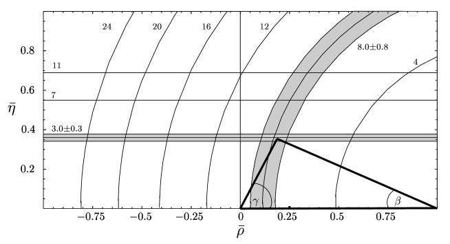
Figure 5: The UT from $K\to\pi\nu\bar{\nu}$ in Scenario I of table 4. Also lines corresponding to several values of $Br(K^{+}\rightarrow\pi^{+}\nu\bar{\nu})$ and $Br(K_{\rm L}\rightarrow\pi^{0}\nu\bar{\nu})$ (in units of $10^{-11}$) are shown.

IV.4 Impact of $Br(K_{\rm L}\rightarrow\pi^{0}\nu\bar{\nu})$ on the UT

IV.4.1 $\bar{\eta}$ and ${\rm Im}\lambda_{t}$

We consider next the impact of a future measurement of $Br(K_{\rm L}\rightarrow\pi^{0}\nu\bar{\nu})$ on the UT. As already discussed in the previous section, this measurement will offer a theoretically clean determinations of $\bar{\eta}$ and in particular of ${\rm Im}\lambda_{t}$. The relevant formulae are given in (III.17) and (III.18), respectively. Using Scenarios I and II of table 4 we find

$$\bar{\eta}=0.367\pm 0.019,\qquad{\rm Im}\lambda_{t}=(1.47\pm 0.07)\cdot 10^{-4}\qquad{\rm(Scenario~{}I)}.$$ (IV.9)

$$\bar{\eta}=0.367\pm 0.013,\qquad{\rm Im}\lambda_{t}=(1.47\pm 0.05)\cdot 10^{-4}.\qquad{\rm(Scenario~{}II)}$$ (IV.10)

The obtained precision in the case of Scenario II is truely impressive. We stress the very clean character of these determinations.

IV.4.2 Completing the Determination of the UT

In order to construct the UT we need still another input. It could be $\beta$, $\gamma$, $R_{b}$ or $R_{t}$. It turns out that the most effective in this determination is $\gamma$, as in the classification of Buras et al. (2003a) the $(\bar{\eta},\gamma)$ strategy belongs to the top class together with the $(\beta,\gamma)$ pair. The angle $\gamma$ should be known with high precision in five years. Still it is of interest to see what one finds when $\beta$ instead of $\gamma$ is used. $R_{b}$ is not useful here as it generally gives two solutions for the UT.

In analogy to table 7 we show in table 8 the values of $\bar{\varrho}$ and $|V_{td}|$ resulting from Scenarios I and II without using $Br(K^{+}\rightarrow\pi^{+}\nu\bar{\nu})$. As an additional variable we use $\beta$ or $\gamma$. We observe that, with the assumed errors on $\beta$ and $\gamma$, the use of $\gamma$ is more effective than the use of $\beta$. Moreover, while going from Scenario I to Scenario II for $Br(K_{\rm L}\rightarrow\pi^{0}\nu\bar{\nu})$ has a significant impact when $\beta$ is used, the impact is rather small when $\gamma$ is used instead. Both features are consistent with the observations made in Buras et al. (2003a) in the context of $(\beta,\bar{\eta})$ and $(\gamma,\bar{\eta})$ strategies. In particular, the last feature is directly related to the fact that $\gamma$ is by a factor of three larger than $\beta$.

The main message from table 8 is that, using a rather precise value of $\gamma$, a very precise determination of $|V_{td}|$ becomes possible, where the branching fraction of $K_{\rm L}\rightarrow\pi^{0}\nu\bar{\nu}$ needs to be known only to about $10\%$ accuracy.

Table 8: The values for $\bar{\varrho}$ and $|V_{td}|/10^{-3}$ (in parentheses) from $K_{\rm L}\rightarrow\pi^{0}\nu\bar{\nu}$ for various cases considered in the text.

	Scenario I	Scenario II
Scenario B ($\beta$)	$0.101\pm 0.052~{}(9.12\pm 0.51)$	$0.101\pm 0.040~{}(9.12\pm 0.37)$
Scenario B ($\gamma$)	$0.174\pm 0.018~{}(8.49\pm 0.16)$	$0.174\pm 0.017~{}(8.49\pm 0.16)$

IV.4.3 A Clean and Accurate Determination of $|V_{cb}|$ and $|V_{td}|$

Next, combining $\beta$ and $\gamma$ with the values of $Br(K_{\rm L}\rightarrow\pi^{0}\nu\bar{\nu})$ and $m_{t}$, a clean determination of $|V_{cb}|$ by means of (III.22) is possible. In turn also $|V_{td}|$ can be determined. In table 9 we show the values of $|V_{cb}|$ and $|V_{td}|$ obtained using Scenarios I and II for $Br(K_{\rm L}\rightarrow\pi^{0}\nu\bar{\nu})$ in table 4 with $\beta$ and $\gamma$ in Scenario B of table 3.

We observe that the errors on $|V_{cb}|$ are larger than presently obtained from semi-leptonic $B$ decays. But one should emphasize that this determination is essentially without any theoretical uncertainties. The high precision on $|V_{td}|$ is a result of a very precise measurement of $R_{t}$ by means of the $(\beta,\gamma)$ strategy and a rather accurate value of $|V_{cb}|$ obtained with the help of $Br(K_{\rm L}\rightarrow\pi^{0}\nu\bar{\nu})$. Again also in this case the determination is theoretically very clean.

Table 9: The values for $|V_{cb}|$ and $|V_{td}|$ (in parentheses) in units of $10^{-3}$ from $K_{\rm L}\rightarrow\pi^{0}\nu\bar{\nu}$, $\beta$ and $\gamma$ for various cases considered in the text.

	Scenario I	Scenario II
Scenario B	$43.1\pm 1.2~{}(8.23\pm 0.76)$	$43.1\pm 0.9~{}(8.23\pm 0.48)$

IV.5 Impact of $Br(K^{+}\rightarrow\pi^{+}\nu\bar{\nu})$ and $Br(K_{\rm L}\rightarrow\pi^{0}\nu\bar{\nu})$ on UT

In Buchalla and Buras (1996) the determination of the UT from both decays has been discussed in explicit terms. The relevant formulae have been given in Section III. Here we confine our discussion to the determination of ${\rm Im}\lambda_{t}$, $\sin 2\beta$ and $\gamma$. We consider again two scenarios for which the input parameters are collected in table 4. This time no other parameters beside those given in this table are required for the construction of the UT and the determination of these three quantities in question.

IV.6 ${\rm Im}\lambda_{t}$ from $K_{\rm L}\rightarrow\pi^{0}\nu\bar{\nu}$

As oposed to $\sin 2\beta$ and $\gamma$ only $K_{\rm L}\rightarrow\pi^{0}\nu\bar{\nu}$ is relevant here. Using (III.18) we find that the error from $m_{t}$ is roughly $1\%$ and will soon be decreased even below that. Neglecting it, we find

$$\frac{\sigma({\rm Im}\lambda_{t})}{{\rm Im}\lambda_{t}}=\pm 0.5\frac{\sigma(Br(K_{L}))}{Br(K_{L})}=\left\{\begin{array}[]{ll}5.0\%&{\rm Scenario\,I}\\ 3.3\%&{\rm Scenario\,II}\end{array}\right.$$ (IV.11)

which already in the case of Scenario II is an impressive accuracy.

IV.7 The Angle $\beta$ from $K\to\pi\nu\bar{\nu}$

Let us next investigate the separate uncertainties in the determination of $\sin 2\beta$ coming from $P_{c}$, $Br(K^{+}\rightarrow\pi^{+}\nu\bar{\nu})\equiv Br(K^{+})$ and $Br(K_{\rm L}\rightarrow\pi^{0}\nu\bar{\nu})\equiv Br(K_{L})$. We find first

$$\frac{\sigma(\sin 2\beta)}{\sin 2\beta}=\pm 0.31\frac{\sigma(P_{c})}{P_{c}}\pm 0.55\frac{\sigma(Br(K^{+}))}{Br(K^{+})}\pm 0.39\frac{\sigma(Br(K_{L}))}{Br(K_{L})}~{}.$$ (IV.12)

This leads to

$$\sigma(\sin 2\beta)=0.030_{P_{c}}+0.041_{Br(K^{+})}+0.029_{Br(K_{L})}=0.080\qquad({\rm Scenario~{}I})$$ (IV.13)

and

$$\sigma(\sin 2\beta)=0.011_{P_{c}}+0.020_{Br(K^{+})}+0.018_{Br(K_{L})}=0.038,\qquad({\rm Scenario~{}II})$$ (IV.14)

where the errors have been added in quadrature apart from the one in $P_{c}$ which has been added linearly. The uncertainties due to $|V_{cb}|$ and $m_{t}$ are fully negligible.

We observe that

• The uncertainty in $\sin 2\beta$ due to $P_{c}$ alone amounted to $0.04$ at NLO, implying that a NNLO calculation of $P_{c}$ was very desirable. On the other hand, now, at NNLO, the pure perturbative uncertainty in $\sin 2\beta$ amounts to $\pm 0.006\%$ Buras et al. (2006a), to be compared with $\pm 0.025\%$ at NLO.

• The accuracy of the determination of $\sin 2\beta$, after the NNLO result became available, depends dominantly on the accuracy with which both branching ratios will be measured. In order to decrease $\sigma(\sin 2\beta)$ down to $0.02$ they have to be measured with an accuracy better than $5\%$. Also, the reduction of the error in $m_{c}$ relevant for $P_{c}$ would be desirable.

IV.8 The Angle $\gamma$ from $K\to\pi\nu\bar{\nu}$

Let us next investigate, in analogy to (IV.12), the separate uncertainties in the determination of $\gamma$ coming from $P_{c}$, $Br(K^{+}\rightarrow\pi^{+}\nu\bar{\nu})$, $Br(K_{\rm L}\rightarrow\pi^{0}\nu\bar{\nu})$ and $|V_{cb}|$. The relevant expression for $\gamma$ in terms of these quantities is given in (III.29). We find then

$$\frac{\sigma(\gamma)}{\gamma}=\pm 0.75\frac{\sigma(P_{c})}{P_{c}}\pm 1.32\frac{\sigma(Br(K^{+}))}{Br(K^{+})}\pm 0.07\frac{\sigma(Br(K_{L}))}{Br(K_{L})}\pm 4.11\frac{\sigma(|V_{cb}|)}{|V_{cb}|}\pm 2.34\frac{\sigma(m_{t})}{m_{t}}.$$ (IV.15)

This gives

$$\sigma(\gamma)=5.7^{\circ}_{P_{c}}+8.2^{\circ}_{Br(K^{+})}+0.4^{\circ}_{Br(K_{L})}+3.7_{|V_{cb}|}^{\circ}+1.5_{m_{t}}^{\circ}=19.6^{\circ}$$ (IV.16)

and

$$\sigma(\gamma)=2.3^{\circ}_{P_{c}}+4.1^{\circ}_{Br(K^{+})}+0.3^{\circ}_{Br(K_{L})}+1.9_{|V_{cb}|}^{\circ}+0.9_{m_{t}}^{\circ}=9.4^{\circ}$$ (IV.17)

for Scenario I and II, respectively, where the errors have been added in quadrature.

We observe that

• The uncertainty in $\gamma$ due to $P_{c}$ alone amounted to $8.6^{\circ}$ at the NLO level, implying that a NNLO calculation of $P_{c}$ was very desirable. The pure perturbative uncertainty in $\gamma$ amounts to $\pm 1.2\%$ at NNLO, compared to $\pm 4.9\%$ at NLO. Again, the reduction of the error in $m_{c}$ relevant for $P_{c}$ would be desirable.

• The dominant uncertainty in the determination of $\gamma$ in Scenarios I and II besides the one of $P_{c}$ resides in $Br(K^{+}\rightarrow\pi^{+}\nu\bar{\nu})$. In order to lower $\sigma(\gamma)$ below $5^{\circ}$, a measurement of this branching ratio with an accuracy of better than $5\%$ is required. The measurement of $Br(K_{\rm L}\rightarrow\pi^{0}\nu\bar{\nu})$ has only a small impact on this determination.

IV.9 Summary

In this section we have presented a very detailed numerical analysis of the formulae of Section III. First working in two scenarios, A and B, for the input parameters that should be measured precisely through $B$ physics observables in this decade, we have shown how the accuracy on the predictions of the branching ratios will improve with time.

In the case of $Br(K_{\rm L}\rightarrow\pi^{0}\nu\bar{\nu})$ there are essentially no theoretical uncertainties and the future of the accuracy of the prediction on this branching ratio within the SM depends fully on the accuracy with which ${\rm Im}\lambda_{t}$ and $m_{t}$ can be determined from other processes. We learn from table 5 that the present error of roughly $12\%$ will be decreased to $6\%$ when the Scenario B will be realized. As seen in table 6, the progress on the error on $Br(K_{\rm L}\rightarrow\pi^{0}\nu\bar{\nu})$ will depend importantly on the progress on $|V_{cb}|$.

The case of $K^{+}\rightarrow\pi^{+}\nu\bar{\nu}$ is a bit different as now also the uncertainty in $P_{c}$ enters. As discussed in Section II, this uncertainty comes on the one hand from the scale uncertainty and on the other hand from the error in $m_{c}$. The scale uncertainty dominated at NLO while the error on $m_{c}$ is mainly responsible for the present error in $P_{c}$ after NNLO has been completed. Formula (II.18) quantifies this explicitely. The anatomy of parametric uncertainties in $Br(K^{+}\rightarrow\pi^{+}\nu\bar{\nu})$ is presented in table 6. As in the case of $Br(K_{\rm L}\rightarrow\pi^{0}\nu\bar{\nu})$ also here the reduction of the error in $|V_{cb}|$ will be important.

As seen in table 5 the present error in $Br(K^{+}\rightarrow\pi^{+}\nu\bar{\nu})$ due to $P_{c}$ amounts roughly to $\pm 8\%$, which is roughly by a factor of 1.5 smaller than before the NNLO results for $P_{c}$ where available. It is also clearly seen in this table that in order to benefit from the improved values of the CKM parameters and of $m_{\rm t}$, also the uncertainty in $P_{c}$ has to be reduced through the improvement of $m_{c}$. It appears to us that the present error of $8\%$ due to $P_{c}$ could be decreased to $3\%$ one day with the present total error of $14\%$ reduced to $7\%$.

In the main part of this section we have investigated the impact of the future measurements of $Br(K^{+}\rightarrow\pi^{+}\nu\bar{\nu})$ and $Br(K_{\rm L}\rightarrow\pi^{0}\nu\bar{\nu})$ on the determination of the CKM matrix. The results are self-explanatory and demonstrate very clearly that the $K\to\pi\nu\bar{\nu}$ decays offer powerful means in the determination of the UT and of the CKM matrix.

Clearly, the future determination of various observables by means of $K\to\pi\nu\bar{\nu}$ will crucially depend on the accuracy with which $Br(K^{+}\rightarrow\pi^{+}\nu\bar{\nu})$ and $Br(K_{\rm L}\rightarrow\pi^{0}\nu\bar{\nu})$ can be measured. Our discussion shows that it is certainly desirable to measure both branching ratios with an accuracy of at least $5\%$.

On the other hand the uncertainties due to $P_{c}$, $|V_{cb}|$ and to a lesser extent $m_{t}$ are also important ingredients of these investigations.

V A Guide to Sections VI-VIII

Until now our discussion was confined to the SM. In the next three sections we will discuss the decays $K\to\pi\nu\bar{\nu}$ in various extensions of the SM.

In the case of most $K$ and $B$ meson decays the effective Hamiltonian in the extensions of the SM becomes generally much more complicated than in the SM in that new operators, new complex phases, and new one-loop short distance functions and generally new flavour violating couplings can be present. A classification of various possible extensions of the SM from the point of view of an effective Hamiltonian and valid for all decays can be found in Buras (2005a).

As we already emphasized at the beginning of this review in the case of $K\to\pi\nu\bar{\nu}$, the effective Hamiltonian in essentially all extensions of the SM is found simply from ${\cal H}^{\rm SM}_{\rm eff}$ in (II.1) by replacing $X(x_{t})$ as follows Buras et al. (1998)

$$X(x_{t})\rightarrow X=\left|X\right|e^{i\theta_{X}}.$$ (V.18)

Thus, the only effect of new physics is to modify the magnitude of the SM function $X(x_{t})$ and/or introduce a new complex phase $\theta_{X}$ that vanishes in the SM.

Clearly, the simplest class of extensions are models with minimal flavour violatio in which $\theta_{X}=0,\pi$ and $\left|X\right|$ is only modified by loop diagrams with new particles exchanges but the driving mechanism of flavour and CP violation remains to be the CKM matrix. As in this class of models the basic structure of effective Hamiltonians in other decays is unchanged relative to the SM and only the modifications in the one-loop functions, analogous to $X$, are allowed, the correlations between $K\to\pi\nu\bar{\nu}$ and other $K-$ and, in particular, $B-$decays, valid in the SM remain true. A detailed review of these correlations has been given in Buras (2003).

In the following section, we will summarize the present status of $K\to\pi\nu\bar{\nu}$ in the models with MFV. As we will see, the recently improved bounds on rare $B$ decays, combined with the correlations in question, do not allow for a large departure of $K\to\pi\nu\bar{\nu}$ from the SM within this simplest class of new physics.

Much more spectacular effects in $K\to\pi\nu\bar{\nu}$ are still possible in models in which the phase $\theta_{X}$ is large. We discuss this in Section VII in a model independent manner. We also discuss there situations in which simultaneously to $\theta_{X}\not=0$, also new complex phases in $B_{d}^{0}-\bar{B}_{d}^{0}$ mixing are present, and illustrate how these new phases, including $\theta_{X}$, could be extracted from future data.

While Section VI and VII have a more model independent character and basically analyze the implications of the replacement (V.18) with arbitrary $\left|X\right|$ and $\theta_{X}$, Section VIII can be considered as a guide to the rich literature on the new physics effects in $K\to\pi\nu\bar{\nu}$. In particular, we discuss the Littlest Higgs Model with T-parity, $Z^{\prime}$ models, the MSSM with MFV, general supersymmetric models, models with universal extra dimensions and models with lepton flavor mixing. Finally, we briefly comment on essentially all new physics analyses done until the summer of 2007.

VI $K\to\pi\nu\bar{\nu}$ and MFV

VI.1 Preliminaries

A general discussion of the decays $K^{+}\rightarrow\pi^{+}\nu\bar{\nu}$ and $K_{\rm L}\rightarrow\pi^{0}\nu\bar{\nu}$ in the framework of minimal flavour violation (MFV) has been presented in Buras and Fleischer (2001). Earlier papers in specific MFV scenarios like two Higgs doublet can be found in Belanger et al. (1992); Cho (1998), where additional references are given. We would like to recall that in almost all extensions of the SM the effective Hamiltonian for $K\to\pi\nu\bar{\nu}$ decays involves only the $(V-A)\otimes(V-A)$ operator of (II.1) and consequently for these decays there is no distinction between the constrained MFV (CMFV) Buras et al. (2001b); Blanke et al. (2006) and more general formulation of MFV D’Ambrosio et al. (2002) in which additional non-SM operators are present in certain decays. Consequently in MFV or CMFV, all formulae of Section II and III for $K\to\pi\nu\bar{\nu}$ remain valid except that

• the function $X(x_{t})$ is replaced by the real valued master function Buras (2005a, 2003, b) $X(v)$ with $v$ denoting collectively the parameters of a given MFV model,

• if the function $X(v)$ is allowed to take also negative values, the following replacements should effectively be made in all formulae of Sections II and III Buras and Fleischer (2001)

  $$X\to|X|,\qquad P_{c}(X)\to{\rm sgn}(X)P_{c}(X).$$ (VI.1)

Here we will also assume that the $B^{0}-\bar{B}^{0}$ function $S(v)>0$, as in the SM. In fact as found recently in Blanke and Buras (2007); Altmannshofer et al. (2007) in all models with CMFV $S(v)>S(v)_{\rm SM}$. On the other hand, we will allow first for negative values of the function $X(v)$. The values of $X(v)$ and $S(v)$ can be calculated in any MFV model.

VI.2 $K^{+}\rightarrow\pi^{+}\nu\bar{\nu}$ versus $K_{\rm L}\rightarrow\pi^{0}\nu\bar{\nu}$

An important consequence of (III.26) and (I.1) is the following MFV relation Buras and Fleischer (2001)

$$B_{1}=B_{2}+\left[\frac{\cot\beta\sqrt{B_{2}}+{\rm sgn}(X)\sqrt{\sigma}P_{c}(X)}{\sigma}\right]^{2},$$ (VI.2)

that, for a given $\sin 2\beta$ extracted from $a_{\psi K_{S}}$ and $Br(K^{+}\rightarrow\pi^{+}\nu\bar{\nu})$, allows to predict $Br(K_{\rm L}\rightarrow\pi^{0}\nu\bar{\nu})$. We observe that in the full class of MFV models, independent of any new parameters present in these models, only two values for $Br(K_{\rm L}\rightarrow\pi^{0}\nu\bar{\nu})$, corresponding to two signs of $X$, are possible. Consequently, measuring $Br(K_{\rm L}\rightarrow\pi^{0}\nu\bar{\nu})$ will either select one of these two possible values or rule out all MFV models. In fact the recent analysis Haisch and Weiler (2007) shows that $X<0$ is basically ruled out and these are good news as $X>0$ gives larger branching ratios for the same $|X|$. We will therefore not consider $X<0$ any further.

In Buras and Fleischer (2001) a detailed numerical analysis of the relation (VI.2) has been presented. In view of the improved data on $\sin 2\beta$ and $Br(K^{+}\rightarrow\pi^{+}\nu\bar{\nu})$ we update and extend this analysis. This is shown in Fig. 6, where we show $Br(K^{+}\rightarrow\pi^{+}\nu\bar{\nu})$ as a function of $Br(K_{\rm L}\rightarrow\pi^{0}\nu\bar{\nu})$ for several values of $a_{\psi K_{S}}$. These plots are universal for all MFV models.

Figure 6: $Br(K^{+}\rightarrow\pi^{+}\nu\bar{\nu})$ as a function of $Br(K_{\rm L}\rightarrow\pi^{0}\nu\bar{\nu})$ for several values of $a_{\psi K_{S}}$ in the case of ${\rm sgn}(X)=1$.

We also observe, as in Buras and Fleischer (2001), that the upper bound on $Br(K_{\rm L}\rightarrow\pi^{0}\nu\bar{\nu})$ following from the data on $Br(K^{+}\rightarrow\pi^{+}\nu\bar{\nu})$ and $\sin 2\beta\leq 0.719$ is substantially stronger than the model independent bound following from isospin symmetry Grossman and Nir (1997)

$$Br(K_{\rm L}\rightarrow\pi^{0}\nu\bar{\nu})<4.4\cdot Br(K^{+}\rightarrow\pi^{+}\nu\bar{\nu}).$$ (VI.3)

With the data in (I.5), that imply

$$Br(K^{+}\rightarrow\pi^{+}\nu\bar{\nu})<3.8\cdot 10^{-10}~{}(90\%~{}\mbox{C.L.}),$$ (VI.4)

one finds from (VI.3)

$$Br(K_{\rm L}\rightarrow\pi^{0}\nu\bar{\nu})<1.7\cdot 10^{-9}~{}(90\%~{}\mbox{C.L.}),$$ (VI.5)

that is still two orders of magnitude lower than the upper bound from the KTeV experiment at Fermilab Blucher (2005), yielding $Br(K_{\rm L}\rightarrow\pi^{0}\nu\bar{\nu})<2.9\cdot 10^{-7}$ and the bound from KEK, $Br(K_{\rm L}\rightarrow\pi^{0}\nu\bar{\nu})<2.1\cdot 10^{-7}$ Ahn et al. (2006).

On the other hand, taking the experimental bound $Br(K^{+}\rightarrow\pi^{+}\nu\bar{\nu})$ in (I.5) and $a_{\psi K_{S}}\leq 0.719$, we find from (VI.2)

$$Br(K_{\rm L}\rightarrow\pi^{0}\nu\bar{\nu})_{\rm MFV}\leq 2.0\cdot 10^{-10},\qquad{\rm sgn}(X)=+1.$$ (VI.6)

In Bobeth et al. (2005) a detailed analysis of several branching ratios for rare $K$ and $B$ decays in MFV models has been performed. Using the presently available information on the UUT, summarized in Bona et al. (2006b), and from the measurements of $Br(B\to X_{s}\gamma)$, $Br(B\to X_{s}l^{+}l^{-})$ and $Br(K^{+}\rightarrow\pi^{+}\nu\bar{\nu})$ the upper bounds on various branching ratios within the CMFV scenario have been found. Very recently this analysis has been updated and generalized to include the constraints from the observables in $Z\to b\bar{b}$ decay Haisch and Weiler (2007). The results of this analysis are collected in Table 10 together with the results within the SM.

Finally, anticipating that the leading role in constraining this kind of physics will eventually be taken over by $K^{+}\rightarrow\pi^{+}\nu\bar{\nu}$, $K_{\rm L}\rightarrow\pi^{0}\nu\bar{\nu}$ and $B_{s,d}\to\mu^{+}\mu^{-}$, that are dominated by the function $C(v)$, references Bobeth et al. (2005); Haisch and Weiler (2007) provide plots for several branching ratios as functions of $C(v)$.

Observable	CMFV ($95\%\,{\rm CL}$)	SM ($68\%\,{\rm CL}$)	SM ($95\%\,{\rm CL}$)	Experiment
${Br}(K^{+}\rightarrow\pi^{+}\nu\bar{\nu})\times 10^{11}$	$[4.29,10.72]$	$7.15\pm 1.28$	$[5.40,9.11]$	$\left(14.7^{+13.0}_{-8.9}\right)$ Anisimovsky et al. (2004)
${Br}(K_{\rm L}\rightarrow\pi^{0}\nu\bar{\nu})\times 10^{11}$	$[1.55,4.38]$	$2.79\pm 0.31$	$[2.21,3.45]$	$<2.1\times 10^{4}\;\;(90\%\,\text{CL})$ Ahn et al. (2006)
${Br}(K_{L}\to\mu^{+}\mu^{-})_{\rm SD}\times 10^{9}$	$[0.30,1.22]$	$0.70\pm 0.11$	$[0.54,0.88]$	–
${Br}(\bar{B}\to X_{d}\nu\bar{\nu})\times 10^{6}$	$[0.77,2.00]$	$1.34\pm 0.05$	$[1.24,1.45]$	–
${Br}(\bar{B}\to X_{s}\nu\bar{\nu})\times 10^{5}$	$[1.88,4.86]$	$3.27\pm 0.11$	$[3.06,3.48]$	$<64\;\;(90\%\,\text{CL})$ Barate et al. (2001)
$Br(B_{d}\to\mu^{+}\mu^{-})\times 10^{10}$	$[0.36,2.03]$	$1.06\pm 0.16$	$[0.87,1.27]$	$<3.0\times 10^{2}\;\;(95\%\,\text{CL})$ Bernhard (2006)
${Br}(B_{s}\to\mu^{+}\mu^{-})\times 10^{9}$	$[1.17,6.67]$	$3.51\pm 0.50$	$[2.92,4.13]$	$<5.8\times 10^{1}\;\;(95\%\,\text{CL})$ Maciel (2007)

Table 10: Bounds for various rare decays in CMFV models at $95\%$ probability, the corresponding values in the SM at $68\%$ and $95\%\,{\rm CL}$, and the available experimental information Haisch and Weiler (2007). See text for details.

The main messages from Bobeth et al. (2005); Haisch and Weiler (2007) are the following ones:

The existing constraints coming from $K^{+}\to\pi^{+}\nu\bar{\nu}$, $B\to X_{s}\gamma$, $B\to X_{s}l^{+}l^{-}$ and $Z\to b\bar{b}$ do not allow within the CMFV scenario of Buras et al. (2001b) for substantial departures of the branching ratios for all rare $K$ and $B$ decays from the SM estimates. This is evident from Table 10.

This could be at first sight a rather pessimistic message. On the other hand it implies that finding practically any branching ratio enhanced by more than a factor of two with respect to the SM will automatically signal either the presence of new CP-violating phases or new operators, strongly suppressed within the SM, at work. In particular, recalling that in most extensions of the SM the decays $K\to\pi\nu\bar{\nu}$ are governed by the single $(V-A)\otimes(V-A)$ operator, the violation of the upper bounds on at least one of the $K\to\pi\nu\bar{\nu}$ branching ratios, will either signal the presence of new complex weak phases at work or new contributions that violate the correlations between the $B$ decays and $K$ decays.

As $a_{\psi K_{S}}$ in MFV models determines the true value of $\beta$ and the true value of $\gamma$ can be determined in tree level strategies in $B$ decays one day, the true value of $\bar{\eta}$ can also be determined in a clean manner. Consequently, using (III.21) offers probably the cleanest measurement of $|X|$ in the field of weak decays.

VII Scenarios with New Complex Phases in $\Delta F=1$ and $\Delta F=2$ Transitions

VII.1 Preliminaries

In this section we will consider three simple scenarios beyond the framework of MFV, in which $X$ becomes a complex quantity as given in (I.7), and the universal box function $S(v)$ entering $\varepsilon_{K}$ and $\Delta M_{d,s}$ not only becomes complex but generally becomes non-universal with

$$S_{K}(v)=|S_{K}(v)|e^{i2\varphi_{K}},\quad S_{d}(v)=|S_{d}(v)|e^{i2\varphi_{d}},\quad S_{s}(v)=|S_{s}(v)|e^{i2\varphi_{s}},$$ (VII.1)

for $K^{0}-\bar{K}^{0}$, $B_{d}^{0}-\bar{B}_{d}^{0}$ and $B_{s}^{0}-\bar{B}_{s}^{0}$ mixing, respectively. If these three functions are different from each other, some universal properties found in the SM and MFV models, that have been reviewed in Buras (2005a, 2003, b), are lost. In addition, the mixing induced CP asymmetries in $B$ decays do not measure the angles of the UT but only sums of these angles and of $\varphi_{i}$. In particular

$$S_{\psi K_{S}}=\sin(2\beta+2\varphi_{B_{d}}).$$ (VII.2)

Equally importantly the rare $K$ and $B$ decays, governed in models with MFV by the real universal functions $X$, $Y$ and $Z$, are described now by nine complex functions ($i=K,d,s$) Blanke et al. (2007b)

$$X_{i}=|X_{i}|e^{i\theta_{K}^{i}},\quad Y_{i}=|Y_{i}|e^{i\theta_{Y}^{i}},\quad Z_{i}=|Z_{i}|e^{i\theta_{Z}^{i}}$$ (VII.3)

that result from th SM box and penguin diagrams and analogous diagrams with new particle exchanges. In the SM and in CMFV models the independence of the functions in (VII.3) of $i$ implies very strong correleations between various branching ratios in $K$, $B_{d}$ and $B_{s}$ system and consequently strong upper bounds as shown in table 10. In models with new complex phases this universality is generally broken and consequently as we will see in the next section the bounds in Table 10 can be strongly violated.

As in the $K\to\pi\nu\bar{\nu}$ system only one function is present, we will drop the index $i$ and denote it by

$$X=|X|e^{i\theta_{X}}.$$ (VII.4)

In order to simplify the presentation we will assume here that $S_{s}=S_{0}(x_{t})$ as in the SM but we will take $S_{d}(v)$ to be complex with $S_{d}(v)\not=S_{0}(x_{t})$. This will allow to change the relation between $R_{t}$ and $\Delta M_{d}/\Delta M_{s}$ in (II.45). We will leave open whether $S_{K}(v)$ receives new physics contributions. We will relax these assumptions in concrete models in the next chapter.

An example of general scenarios with new complex phases is the scenario in which new physics enters dominantly through enhanced $Z^{0}$ penguins involving a new CP-violating weak phase. It was first considered in Buras et al. (1998); Colangelo and Isidori (1998); Buras and Silvestrini (1999); Buras et al. (2000) in the context of rare $K$ decays and the ratio $\varepsilon^{\prime}/\varepsilon$ measuring direct CP violation in the neutral kaon system, and was generalized to rare $B$ decays in Buchalla et al. (2001); Atwood and Hiller (2003). Subsequently this particular extension of the SM has been revived in Buras et al. (2004b, a), where it has been pointed out that the anomalous behaviour in $B\to\pi K$ decays observed by CLEO, BABAR and Belle Bornheim et al. (2003); Aubert et al. (2002b, 2004, 2003); Chao et al. (2004) could be due to the presence of enhanced $Z^{0}$ penguins carrying a large new CP-violating phase around $-90^{\circ}$.

The possibility of important electroweak penguin contributions behind the anomalous behaviour of the $B\to\pi K$ data has been pointed out already in Buras and Fleischer (2000), but only in 2005 has this behaviour been independently observed by the three collaborations in question. Recent discussions related to electroweak penguins can be also found in Yoshikawa (2003); Beneke and Neubert (2003). Other conjectures in connection with these data can be found in Gronau and Rosner (2003b, a); Chiang et al. (2004).

The implications of the large CP-violating phase in electroweak penguins for rare $K$ and $B$ decays and $B\to X_{s}l^{+}l^{-}$ have been analyzed in detail in Buras et al. (2004b, a) and subsequently the analyses of $B\to X_{s}l^{+}l^{-}$ and $K_{L}\to\pi^{0}l^{+}l^{-}$ have been extended in Rai Choudhury et al. (2004) and Isidori et al. (2004), respectively. It turns out that in this scenario several predictions differ significantly from the SM expectations with most spectacular effects found precisely in the $K\to\pi\nu\bar{\nu}$ system.

Meanwhile the data on $B\to\pi K$ decays have changed considerably and the case for large electroweak penguin contributions in these decays is much less convincing Fleischer et al. (2007); Fleischer (2007); Baek and London (0100); Silvestrini (2007); Gronau and Rosner (2006); Jain et al. (0600). Still the general formalism developed for the $K\to\pi\nu\bar{\nu}$ system in the presence of new complex phases Buras (1998) and Buras et al. (2004b, a) remains valid and we will present it below. Moreover, in the next section we will discuss three explicit models, Littlest Higgs model with T-Parity (LHT), a $Z^{\prime}$ model and the MSSM in which the functions $X$ becomes a complex quantity and the departures of the $K\to\pi\nu\bar{\nu}$ rates from the SM ones can be spectacular.

The scenarios with complex phases in $B^{0}_{d}-\bar{B}^{0}_{d}$ mixing have been considered in many papers with the subset of references given in D’Ambrosio and Isidori (2002); Bergmann and Perez (2001, 2000); Bertolini et al. (1987); Nir and Silverman (1990a, b); Laplace et al. (2002); Laplace (2002), Fleischer et al. (2003); Bona et al. (2006b).

Very recently this scenario has been revived through the possible inconsistencies between UUT and the RUT signalled by the discrepancy between the value of $\sin 2\beta$ from $S_{\psi K_{S}}$ and its value obtained from tree-level measurements. We will return to this issue below.

In what follows, we will first briefly review the formulae for $K^{+}\rightarrow\pi^{+}\nu\bar{\nu}$ and $K_{\rm L}\rightarrow\pi^{0}\nu\bar{\nu}$ decays obtained in Buras et al. (2004b, a), for the case of a complex $X$. Subsequently, we will discuss the implications of this general scenario for the relevant branching ratios.

Next we will consider scenarios with new physics present only in $B^{0}_{d}-\bar{B}^{0}_{d}$ mixing and the function $X$ as in the SM. Here the impact on $Br(K^{+}\rightarrow\pi^{+}\nu\bar{\nu})$ and $Br(K_{\rm L}\rightarrow\pi^{0}\nu\bar{\nu})$ comes only through modified values of the CKM parameters but, as we will see below, this impact is rather interesting.

Finally we will consider a hybrid scenario with new physics entering both $K\to\pi\nu\bar{\nu}$ decays and $B^{0}_{d}-\bar{B}^{0}_{d}$ mixing. In this discussion the $(R_{b},\gamma)$ strategy (RUT) for the determination of the UT will play a very important role.

VII.2 A Large New CP-Violating Phase $\theta_{X}$

In this general scenario the function $X$ becomes a complex quantity Buras et al. (1998), as given in (I.7), with $\theta_{X}$ being a new complex phase that originates from new physics contributions to the relevant Feynman diagrams. Explicit realizations of such extension of the SM will be discussed in Section VIII. In what follows it will be useful to define the following combination of weak phases,

$$\beta_{X}\equiv\beta-\beta_{s}-\theta_{X}=\beta_{\rm eff}-\theta_{X}.$$ (VII.5)

Following Buras et al. (2004a), the branching ratios for $K^{+}\rightarrow\pi^{+}\nu\bar{\nu}$ and $K_{\rm L}\rightarrow\pi^{0}\nu\bar{\nu}$ are now given as follows:

$${Br}(K^{+}\rightarrow\pi^{+}\nu\bar{\nu})=\kappa_{+}\left[\tilde{r}^{2}A^{4}R_{t}^{2}|X|^{2}+2\tilde{r}\bar{P}_{c}(X)A^{2}R_{t}|X|\cos\beta_{X}+\bar{P}_{c}(X)^{2}\right]$$ (VII.6)

$$Br(K_{\rm L}\rightarrow\pi^{0}\nu\bar{\nu})=\kappa_{L}\tilde{r}^{2}A^{4}R_{t}^{2}|X|^{2}\sin^{2}\beta_{X},$$ (VII.7)

with $\kappa_{+}$ given in (II.3), $\kappa_{L}$ given in (II.20), $\bar{P}_{c}(X)$ defined in (III.2), $\beta_{X}$ in (VII.5) and $\tilde{r}$ in (II.27).

Once $Br(K^{+}\rightarrow\pi^{+}\nu\bar{\nu})$ and $Br(K_{\rm L}\rightarrow\pi^{0}\nu\bar{\nu})$ have been measured, the parameters $|X|$ and $\beta_{X}$ can be determined, subject to ambiguities that can be resolved by considering other processes, such as the non-leptonic $B$ decays and the rare decays discussed in Buras et al. (2004a). Combining (VII.6) and (VII.7), the generalization of (III.27) to the scenario considered can be found Buras et al. (2004a); Buras et al. (1998)

$$\sin 2\beta_{X}=\frac{2\bar{r}_{s}}{1+\bar{r}_{s}^{2}},\qquad\bar{r}_{s}=\frac{\varepsilon_{1}\sqrt{B_{1}-B_{2}}-\bar{P}_{c}(X)}{\varepsilon_{2}\sqrt{B_{2}}}=\cot\beta_{X},$$ (VII.8)

where $\varepsilon_{i}=\pm 1$. Moreover,

$$|X|=\frac{\varepsilon_{2}\sqrt{B_{2}}}{\tilde{r}A^{2}R_{t}\sin\beta_{X}},\quad\varepsilon_{2}\sin\beta_{X}>0.$$ (VII.9)

The “reduced” branching ratios $B_{i}$ are given in (III.24).

These formulae are valid for arbitrary $\beta_{X}\not=0^{\circ}$. For $\theta_{X}=0^{\circ}$ and $\varepsilon_{1}=\varepsilon_{2}=1$, one obtains from (III.27) the SM result in (III.27). On the other hand for $99^{\circ}\leq\beta_{X}\leq 125^{\circ}$ one has $\varepsilon_{1}=-1$ and $\varepsilon_{2}=1$.

As in this scenario it is assumed that there are no significant contributions to $B_{s,d}^{0}-\bar{B}_{s,d}^{0}$ mixings and $\varepsilon_{K}$, in particular no complex phases, the determination of the CKM parameters through the standard analysis of the unitarity triangle proceeds as in the SM with the input parameters given in Section II.5. Consequently, $\beta$ and $\beta_{s}$ are already known from the usual analysis of the UT and the measurement of $\bar{r}_{s}$ in $K\to\pi\nu\bar{\nu}$ decays will provide a theoretically clean determination of $\theta_{X}$ and $\beta_{X}$. Similarly, a clean determination of $|X|$ can be obtained from (VII.9), with $R_{t}$ determined by means of (II.35).

It has been pointed out in Buras et al. (2004b) that in the case of $\beta_{X}\approx 90^{\circ}$, in spite of the enhanced value of $|X|$, $Br(K^{+}\rightarrow\pi^{+}\nu\bar{\nu})$ does not significantly differ from the SM estimate because the enhancement of the first term in (VII.6) can be to a large extent compensated by the suppression of the second term ($\cos\beta_{X}\ll\cos(\beta-\beta_{s})$). Consequently, $Br(K^{+}\rightarrow\pi^{+}\nu\bar{\nu})$ in this case is very strongly dominated by the “top” contribution given by the function $X$ and charm-top interference is either small or even destructive.

On the other hand, $\beta_{X}\approx 90^{\circ}$ implies a spectacular enhancement of $Br(K_{\rm L}\rightarrow\pi^{0}\nu\bar{\nu})$ by one order of magnitude. Consequently, while $Br(K_{\rm L}\rightarrow\pi^{0}\nu\bar{\nu})\approx(1/3)Br(K^{+}\rightarrow\pi^{+}\nu\bar{\nu})$ in the SM, it is substantially larger than $Br(K^{+}\rightarrow\pi^{+}\nu\bar{\nu})$ in such a scenario. The huge enhancement of $Br(K_{\rm L}\rightarrow\pi^{0}\nu\bar{\nu})$ seen here is mainly due to the large weak phase $\beta_{X}$, as

$$\frac{Br(K_{\rm L}\rightarrow\pi^{0}\nu\bar{\nu})}{Br(K_{\rm L}\rightarrow\pi^{0}\nu\bar{\nu})_{\rm SM}}=\left|\frac{X}{X_{\rm SM}}\right|^{2}\left[\frac{\sin\beta_{X}}{\sin(\beta-\beta_{s})}\right]^{2}$$ (VII.10)

and to a lesser extent due to the enhanced value of $|X|$, which generally could be bounded by other processes.

Inspecting (VII.6) and (VII.7), one observes Buras et al. (2004a) that the very strong dominance of the “top” contribution in these expressions implies a simple approximate expression:

$$\frac{Br(K_{\rm L}\rightarrow\pi^{0}\nu\bar{\nu})}{Br(K^{+}\rightarrow\pi^{+}\nu\bar{\nu})}\approx 4.4\times(\sin\beta_{X})^{2}\approx 4.2\pm 0.2.$$ (VII.11)

We note that $Br(K_{\rm L}\rightarrow\pi^{0}\nu\bar{\nu})$ is then rather close to its model-independent upper bound Grossman and Nir (1997) given in (VI.3). It is evident from (VII.8) that this bound is reached when the reduced branching ratios $B_{1}$ and $B_{2}$ in (III.24) are equal to each other.

A spectacular implication of such a scenario is a strong violation of the MFV relation Buchalla and Buras (1994b) in (I.1). Indeed, with $\beta_{X}\approx\pm 90^{\circ}$

$$(\sin 2\beta)_{\pi\nu\bar{\nu}}=\sin 2\beta_{X}\neq(\sin 2\beta)_{\psi K_{\rm S}}=0.675\pm 0.026.$$ (VII.12)

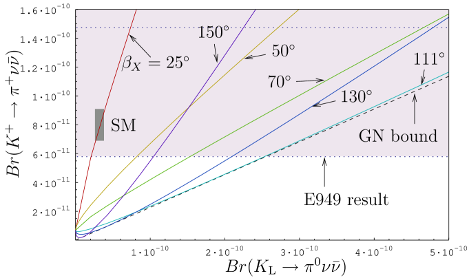
Figure 7: $Br(K^{+}\rightarrow\pi^{+}\nu\bar{\nu})$ as a function of $Br(K_{\rm L}\rightarrow\pi^{0}\nu\bar{\nu})$ for various values of $\beta_{X}$ Buras et al. (2004a). The dotted horizontal lines indicate the lower part of the experimental range (I.4) and the grey area the SM prediction. We also show the bound in (VI.3).

In the next section, we will investigate this violation in two specific models. In Fig. 7, we show – in the spirit of the plot in Fig. 6 – $Br(K^{+}\rightarrow\pi^{+}\nu\bar{\nu})$ as a function of $Br(K_{\rm L}\rightarrow\pi^{0}\nu\bar{\nu})$ for fixed values of $\beta_{X}$ that has been presented in Buras et al. (2004a). As this plot is independent of $|X|$, it offers a direct measurement of the phase $\beta_{X}$. The first line on the left represents the MFV models with $\beta_{X}=\beta_{\rm eff}=\beta-\beta_{s}$, already discussed in Section VI, whereas the first line on the right corresponds to the model-independent Grossman–Nir bound Grossman and Nir (1997) given in (VI.3). Note that the value of $\beta_{X}$ corresponding to this bound depends on the actual value of $Br(K^{+}\rightarrow\pi^{+}\nu\bar{\nu})$ and $Br(K_{\rm L}\rightarrow\pi^{0}\nu\bar{\nu})$ as at this bound ($B_{1}=B_{2}$) we have Buras et al. (2004a)

$$(\cot\beta_{X})_{\rm Bound}=-\frac{\bar{P}_{c}(X)}{\varepsilon_{2}\sqrt{B_{2}}}.$$ (VII.13)

For the central values of $\bar{P}_{c}(X)$ and $B_{2}$ found in the latter paper the bound corresponds to $\beta_{X}=107.3^{\circ}$. As only $\cot\beta_{X}$ and not $\beta_{X}$ is directly determined by the values of the branching ratios in question, the angle $\beta_{X}$ is determined only up to discrete ambiguities, seen already in Fig. 7. These ambiguities can be resolved by considering simultaneously other quantities discussed in Buras et al. (2004a).

VII.3 General Discussion of $\theta_{X}$ and $|X|$

In Fig. 8, we show the ratio of the two branching ratios in question as a function of $\beta_{X}$ for three values of $|X|=1.25,~{}1.5,~{}2.0$. We observe that for $\beta_{X}$ in the ballpark of $110^{\circ}$ this ratio is very close to the bound in (VI.3). However, even for $\beta_{X}=50^{\circ}$ the ratio is close to unity and by a factor of 3 higher than in the SM.

Figure 8: The ratio of the $K\to\pi\nu\bar{\nu}$ branching ratios as a function of $\beta_{X}$ for $|X|=1.25,~{}1.5,~{}2.0$. The horizontal line is the bound in (VI.3).

Finally, in table 11, we give the values of $Br(K^{+}\rightarrow\pi^{+}\nu\bar{\nu})$ and $Br(K_{\rm L}\rightarrow\pi^{0}\nu\bar{\nu})$ for different values of $|X|$ and $\theta_{X}$, $\beta=22.2^{\circ}$ and $|V_{cb}|=41.6\cdot 10^{-3}$. In this context we would like to refer to scaling laws for FCNC processes pointed out in Buras and Harlander (1992), from which it follows that the dependence of $K\to\pi\nu\bar{\nu}$ branching ratios on $|V_{cb}|$ and $|X|$ is encoded in a single variable

$$Z=A^{2}|X|.$$ (VII.14)

This observation allows to make the following replacement in table 11

$$|X|\to|X|_{\rm eff}=\left[\frac{|V_{cb}|}{41.5\cdot 10^{-3}}\right]^{2}|X|,$$ (VII.15)

so that for $|V_{cb}|\not=41.6\cdot 10^{-3}$ the results in this table correspond to different values of $|X|$ obtained by rescaling the values for $|X|$ there by means of (VII.15).

As beyond the SM the uncertainties in the value of $|X|$ are substantially larger than the ones in $|V_{cb}|$, the error in $|V_{cb}|$ can be absorbed into the one of $|X|_{\rm eff}$.

Table 11: Values of $Br(K^{+}\rightarrow\pi^{+}\nu\bar{\nu})$ and of $Br(K_{\rm L}\rightarrow\pi^{0}\nu\bar{\nu})$ (in parentheses) in units of $10^{-11}$ for different values of $\theta_{X}$ and $|X|$ with $\beta=22.2^{\circ}$ and $|V_{cb}|=41.6\cdot 10^{-3}$.

$\theta_{X}/|X|$	$1.25$	$1.50$	$1.75$	$2.00$	$2.25$
$-90^{\circ}$	$2.3$	$3.3$	$4.5$	$6.0$	$7.6$
	$(10.1)$	$(14.5)$	$(19.8)$	$(25.8)$	$(32.7)$
$-60^{\circ}$	$3.8$	$5.0$	$6.5$	$8.3$	$10.2$
	$(12.1)$	$(17.4)$	$(23.6)$	$(30.9)$	$(39.1)$
$-30^{\circ}$	$5.1$	$6.7$	$8.4$	$10.4$	$12.6$
	$(8.1)$	$(11.6)$	$(15.8)$	$(20.7)$	$(26.1)$
$0^{\circ}$	$6.0$	$7.8$	$9.7$	$11.9$	$14.3$
	$(2.1)$	$(3.0)$	$(4.1)$	$(5.4)$	$(6.8)$
$30^{\circ}$	$6.3$	$8.0$	$10.0$	$12.3$	$14.7$
	$(0.11)$	$(0.16)$	$(0.22)$	$(0.29)$	$(0.36)$
$60^{\circ}$	$5.8$	$7.4$	$9.3$	$11.5$	$13.8$
	$(4.1)$	$(5.9)$	$(8.0)$	$(10.5)$	$(13.3)$
$90^{\circ}$	$4.6$	$6.1$	$7.8$	$9.7$	$11.8$
	$(10.1)$	$(14.5)$	$(19.8)$	$(25.8)$	$(32.7)$

VII.4 New Complex Phases in the $B^{0}_{d}-\bar{B}^{0}_{d}$ Mixing

We next move to the scenario in which $X=X_{\rm SM}$ but there are new contributions to $B^{0}_{d}-\bar{B}^{0}_{d}$ mixing. This scenario has been considered in detail in many papers D’Ambrosio and Isidori (2002); Bergmann and Perez (2001, 2000); Bertolini et al. (1987); Nir and Silverman (1990a, b); Laplace et al. (2002); Laplace (2002); Fleischer et al. (2003). As summarized in the latter paper, this scenario can be realized in supersymmetric models with a) a heavy scale for the soft-breaking terms, b) new sources of flavour symmetry breaking only in the soft-breaking terms which do not involve the Higgs fields and c) Yukawa interactions very similar to the SM case. However, as emphasized in Fleischer et al. (2003) and discussed briefly in Section VIII, this scenario is not representative for all supersymmetric scenarios, in particular those with important mass insertions of the left-right type and Higgs mediated FCNC amplitudes with large $\tan\beta$. Non-supersymmetric examples like Littlest Higgs with T-Parity and $Z^{\prime}$-models can also provide new phase effects in $B^{0}_{d}-\bar{B}^{0}_{d}$ mixing but generally such effects are simultaneously present in $B^{0}_{s}-\bar{B}^{0}_{s}$ mixing and $K\to\pi\nu\bar{\nu}$.

Let us recall that, in the presence of a complex function $S_{d}$, the off-diagonal term $M^{d}_{12}$ in the neutral $B^{0}_{d}$ meson mass matrix has the phase structure

$$M^{d}_{12}=\frac{\langle B^{0}_{d}|H_{eff}^{\Delta B=2}|\bar{B}^{0}_{d}\rangle}{2m_{B_{d}}}\propto e^{i2\beta}e^{i2\varphi_{d}}|S_{d}|$$ (VII.16)

with $|S_{d}|$ generally differing from $S_{0}(x_{t})$. If $S_{s}$ remains unchanged, then

• The asymmetry $a_{\psi K_{S}}$ does not measure $\beta$ but $\beta+\varphi_{d}$

• The expression for $R_{t}$ in (II.45) becomes

  $$r_{d}R_{t}=0.920~{}\tilde{r}\left[\frac{\xi}{1.24}\right]\left[\frac{0.2248}{\lambda}\right]\sqrt{\frac{18.4/ps}{\Delta M_{s}}}\sqrt{\frac{\Delta M_{d}}{0.50/ps}},\qquad r^{2}_{d}\equiv\left|\frac{S_{d}}{S_{0}(x_{t})}\right|.$$ (VII.17)

As a consequence of these changes, the true angle $\beta$ differs from the one extracted from $a_{\psi K_{S}}$ and also $R_{t}$ and $|V_{td}|$ will be modified if $r_{d}\not=1$.

As $X$ is not modified with respect to the SM, the impact on $K\to\pi\nu\bar{\nu}$ amounts exclusively to the change of the true $\beta_{\rm eff}$ and $R_{t}$ in the formulae (III.1) and (III.15). A particular pattern of a possible impact on $K\to\pi\nu\bar{\nu}$ in the scenario in question has been presented in Fleischer et al. (2003).

In the meantime the data on the CP asymmetry $S_{\psi K_{S}}$ and the observables in $B_{s,d}^{0}-\bar{B}_{s,d}^{0}$ systems have so much improved that the allowed values for $r_{d}$ and $\varphi_{B_{d}}$ are strongly constrained. Also, there is now a slight tension between the values of $|V_{ub}|$ and $\sin 2\beta$ as inputed into the fits, potentially hinting towards some non-vanishing (negative) phase $\varphi_{B_{d}}$ Bona et al. (2006c); Blanke et al. (2006). However, since there are some open questions concerning the value of $|V_{ub}|$, it remains to be seen how this situation develops further. The implication of this for the $K\to\pi\nu\bar{\nu}$ decays is that, due to the higher value of $\bar{\eta}$ obtained from the RUT fit, the values for both branching ratios are larger than found using CKM values from an overall fit of the unitarity triangle.

VII.5 A Hybrid Scenario

The situation is more involved if new physics effects enter both $X$ and $S$. Similarly to previous two scenarios, the golden relation in (I.1) is violated, but now the structure of a possible violation is more involved

$$\left[\sin 2(\beta-\theta_{X})\right]_{\pi\nu\bar{\nu}}\not=\left[\sin 2(\beta+\varphi_{d})\right]_{\psi K_{S}}.$$ (VII.18)

Since $\theta_{X}$ originates in new contributions to the decay amplitude $K\to\pi\nu\bar{\nu}$ and $\theta_{d}$ in new contributions to the $B^{0}_{d}-\bar{B}^{0}_{d}$ mixing, it is very likely that $\theta_{X}\not=\varphi_{d}$.

The most straightforward strategy to disentangle new physics contributions in $K\to\pi\nu\bar{\nu}$ and the $B^{0}_{d}-\bar{B}^{0}_{d}$ mixing in this scenario is to use the reference unitarity triangle that results from the $(R_{b},\gamma)$ strategy. Having the true CKM parameters at hand, one can determine $\theta_{X}$ and $|X|$ from $K\to\pi\nu\bar{\nu}$ and $\varphi_{d}$ and $|S_{d}|$ from the $B^{0}_{d}-\bar{B}^{0}_{d}$ mixing and $a_{\psi K_{S}}$.

In order to illustrate these ideas in explicit terms let us investigate, in the rest of this section, how the presence of new contributions in $K\to\pi\nu\bar{\nu}$ and the $B^{0}_{d}-\bar{B}^{0}_{d}$ mixing could be signaled in the $(\bar{\varrho},\bar{\eta})$ plane.

Beginning with $K\to\pi\nu\bar{\nu}$, let us write

$$X=r_{X}X_{\rm SM}e^{i\theta_{X}}.$$ (VII.19)

Then formulae (VII.6) and (VII.7) apply with

$$|X|\to X_{\rm SM},\qquad R_{t}\to r_{X}R_{t}.$$ (VII.20)

We proceed then as follows:

• ¿From the measured $Br(K^{+}\rightarrow\pi^{+}\nu\bar{\nu})$ and $Br(K_{\rm L}\rightarrow\pi^{0}\nu\bar{\nu})$ we determine the “fake” angle $\beta$ in the unitarity triangle with the help of (VII.8). We denote this angle by $\beta_{X}$, that we defined in (VII.5). In what follows we neglect $\beta_{s}$ but it can be taken straightforwardly into account if necessary.

• The height of the fake UT from $K\to\pi\nu\bar{\nu}$ is then given by

  $$\bar{\eta}_{\pi\nu\bar{\nu}}=r_{X}R_{t}\sin\beta_{X}=\frac{\sqrt{B_{2}}}{\tilde{r}A^{2}X_{\rm SM}},$$ (VII.21)

  where we set $\varepsilon_{2}=+1$ in order to be concrete. As seen this height can be found from $Br(K_{\rm L}\rightarrow\pi^{0}\nu\bar{\nu})$ and $X_{\rm SM}$.

Now let us go to the $B^{0}_{d}-\bar{B}^{0}_{d}$ mixing where we introduced the parameter $r_{d}$ defined in (VII.17). We proceed then as follows:

• The asymmetry $a_{\psi K_{S}}$ determines the fake angle $\beta$, that we denote by $\beta_{d}=\beta+\theta_{d}$.

• The fake side $R_{t}$, to be denoted by $(R_{t})_{d}$, is now given as follows

  $$(R_{t})_{d}=r_{d}R_{t}.$$ (VII.22)

  It can be calculated from (VII.17) subject to uncertainties in $\xi$.

Clearly, generally the fake UT’s resulting from $K\to\pi\nu\bar{\nu}$ and the $(\Delta M_{d}/\Delta M_{s},\beta)$ strategy, discussed above, will differ from each other, from the true reference triangle and also from the UT obtained from the $(\gamma,\beta)$ and $(\bar{\eta},\gamma)$ strategies, if the determinations of $\bar{\eta}$ and $\beta$ are polluted by new physics.

We show these five different triangles in Fig. 9. Comparing the fake triangles with the reference triangle, all new physics parameters in $K\to\pi\nu\bar{\nu}$ and $B^{0}_{d}-\bar{B}^{0}_{d}$ mixing can be easily extracted. Fig. 9 has only illustrative character. We know already from the recent analyses og the UT Blanke et al. (2006); Bona et al. (2006c) that the phase $\varphi_{B_{d}}$ is constrained to be much smaller than depicted in this figure. Moreover, a negative value seems to be favoured.

Figure 9: Fake unitarity triangles as discussed in the text compared to the reference triangle. $\Delta\beta_{X}=-\theta_{X}$.

VII.6 Correlation between $Br(K_{\rm L}\rightarrow\pi^{0}\nu\bar{\nu})$ and $Br(B\to X_{s,d}\nu\overline{\nu})$

The branching ratios for the inclusive rare decays $B\to X_{s,d}\nu\overline{\nu}$ can be written in the models with a new complex phase in $X$ as follows Buras et al. (2004a) $(q=d,s)$

$$Br(B\to X_{q}\nu\overline{\nu})=1.58\cdot 10^{-5}\left[\frac{Br(B\to X_{c}e\overline{\nu})}{0.104}\right]\left|\frac{V_{tq}}{V_{cb}}\right|^{2}\left[\frac{0.54}{f(z)}\right]~{}|X|^{2},$$ (VII.23)

where $f(z)=0.54\pm 0.04$ is the phase-space factor for $B\to X_{c}e\overline{\nu}$ with $z=m_{c}^{2}/m_{b}^{2}$, and $Br(B\to X_{c}e\overline{\nu})=0.104\pm 0.004$.

Formulae (VII.7) and (VII.23) imply interesting relations between the decays $K_{\rm L}\rightarrow\pi^{0}\nu\bar{\nu}$ and $B\to X_{s,d}\nu\overline{\nu}$ that are generalizations of similar relations within the MFV models Buras and Fleischer (2001); Bergmann and Perez (2001, 2000) to the scenario considered here

$$\frac{Br(K_{\rm L}\rightarrow\pi^{0}\nu\bar{\nu})}{Br(B\to X_{s}\nu\bar{\nu})}=\frac{\kappa_{L}}{1.58\cdot 10^{-5}}\left[\frac{0.104}{Br(B\to X_{c}e\bar{\nu})}\right]\left[\frac{f(z)}{0.54}\right]A^{4}R_{t}^{2}\sin^{2}\beta_{X},$$ (VII.24)

$$\frac{Br(K_{\rm L}\rightarrow\pi^{0}\nu\bar{\nu})}{Br(B\to X_{d}\nu\bar{\nu})}=\frac{\kappa_{L}}{1.58\cdot 10^{-5}}\left[\frac{0.104}{Br(B\to X_{c}e\bar{\nu})}\right]\left[\frac{f(z)}{0.54}\right]\frac{A^{4}\tilde{r}^{2}}{\lambda^{2}}\sin^{2}\beta_{X}.$$ (VII.25)

The experimental upper bound on $Br(B\to X_{s}\nu\overline{\nu})$ reads Barate et al. (2001)

$$Br(B\to X_{s}\nu\overline{\nu})<6.4\cdot 10^{-4}\quad(90\%~{}\mbox{C.L.}).$$ (VII.26)

Using this bound and setting $R_{t}=0.95$, $f(z)=0.58$ and $Br(B\to X_{c}e\overline{\nu})=0.10$, we find from (VII.24) the upper bound

$$Br(K_{\rm L}\rightarrow\pi^{0}\nu\bar{\nu})\leq 4.4\cdot 10^{-9}(\sin\beta_{X})^{2}=\left\{\begin{array}[]{ll}6.3\cdot 10^{-10}&\beta_{X}=22.2^{\circ}\\ 3.9\cdot 10^{-9}&\beta_{X}=111^{\circ}\end{array}\right.$$ (VII.27)

at $90\%~{}\mbox{C.L.}$ for the MFV models and a scenario with a large new phase, respectively. In the case of the MFV models this bound is weaker than the bound in (VI.6) but, as the bound in (VII.26) should be improved in the $B$-factory era, the situation could change in the next years. Concerning the scenario with a complex phase $\theta_{X}$ of Section VII.2, no useful bound on $Br(K_{\rm L}\rightarrow\pi^{0}\nu\bar{\nu})$ from (VII.26) results at present as the bound in (VII.27) is weaker than the model independent bound in (VI.5).

VIII $K\to\pi\nu\bar{\nu}$ in Selected New Physics Scenarios

VIII.1 Preliminaries

In this section we will briefly review the results for decays $K^{+}\rightarrow\pi^{+}\nu\bar{\nu}$ and $K_{\rm L}\rightarrow\pi^{0}\nu\bar{\nu}$ in selected new physics scenarios. Our goal is mainly to indicate the size of new physics contributions in the branching ratios in question. Due to several free parameters present in some of these extensions the actual predictions for the branching ratios are not very precise and often depend sensitively on some of the parameters involved. The latter could then be determined or bounded efficiently once precise data on $K\to\pi\nu\bar{\nu}$ and other rare decays will be available. While we will only present the results for $Br(K^{+}\rightarrow\pi^{+}\nu\bar{\nu})$ and $Br(K_{\rm L}\rightarrow\pi^{0}\nu\bar{\nu})$, most of the analyses discussed below used all available constraints from other observables known at the time of a given analysis. A detailed analysis of these constraints is clearly beyond the scope of this review. A general discussion of $K\to\pi\nu\bar{\nu}$ beyond the SM can be found in Grossman and Nir (1997). In writing this section we also benefited from Isidori (2003); D’Ambrosio and Isidori (2002); Bryman et al. (2006).

VIII.2 Littlest Higgs Models

One of the most attractive solutions to the so-called little hierarchy problem that affects the Standard Model (SM) is provided by Little Higgs models. They are perturbatively computable up to $\sim 10$ TeV and have a rather small number of parameters, although their predictivity can be weakened by a certain sensitivity to the unknown ultraviolet (UV) completion of the theory. In these models, in contrast to supersymmetry, the problematic quadratic divergences to the Higgs mass are cancelled by loop contributions of new particles with the same spin-statistics of the SM ones and with masses around 1 TeV.
The basic idea of Little Higgs models Arkani-Hamed et al. (2001) is that the Higgs is naturally light as it is identified with a Nambu-Goldstone boson of a spontaneously broken global symmetry.

The most economical, in matter content, Little Higgs model is the Littlest Higgs (LH) model Arkani-Hamed et al. (2002), where the global group $SU(5)$ is spontaneously broken into $SO(5)$ at the scale $f\approx\mathcal{O}(1{\rm TeV})$ and the electroweak sector of the SM is embedded in an $SU(5)/SO(5)$ non-linear sigma model. Gauge and Yukawa Higgs interactions are introduced by gauging the subgroup of $SU(5)$: $[SU(2)\times U(1)]_{1}\times[SU(2)\times U(1)]_{2}$. In the LH model, the new particles appearing at the TeV scales are the heavy gauge bosons ($W^{\pm}_{H},Z_{H},A_{H}$), the heavy top ($T$) and the scalar triplet $\Phi$.

In the original Littlest Higgs model (LH) Arkani-Hamed et al. (2002), the custodial $SU(2)$ symmetry, of fundamental importance for electroweak precision studies, is unfortunately broken already at tree level, implying that the relevant scale of new physics, $f$, must be at least 2-3 TeV in order to be consistent with electroweak precision data Han et al. (2003b); Csaki et al. (2003); Hewett et al. (2003); Chen and Dawson (2004b, a); Yue and Wang (2004); Kilian and Reuter (2004); Han et al. (2003a). As a consequence, the contributions of the new particles to FCNC processes turn out to be at most $10-20\%$ Buras et al. (2005d); Choudhury et al. (2004); Buras et al. (2005c); Huo and Zhu (2003); Buras et al. (2006b), which will not be easy to distinguish from the SM due to experimental and theoretical uncertainties. In particular, a detailed analysis of particle-antiparticle mixing in the LH model has been published in Buras et al. (2005d) and the corresponding analysis of rare $K$ and $B$ decays has recently been presented in Buras et al. (2006b).

More promising and more interesting from the point of view of FCNC processes is the Littlest Higgs model with a discrete symmetry (T-parity) Cheng and Low (2003, 2004) under which all new particles listed above, except $T_{+}$, are odd and do not contribute to processes with external SM quarks (T-even) at tree level. As a consequence, the new physics scale $f$ can be lowered down to 1 TeV and even below it, without violating electroweak precision constraints Hubisz et al. (2006b).

A consistent and phenomenologically viable Littlest Higgs model with T-parity (LHT) requires the introduction of three doublets of “mirror quarks” and three doublets of “mirror leptons” which are odd under T-parity, transform vectorially under $SU(2)_{L}$ and can be given a large mass. Moreover, there is an additional heavy $T_{-}$ quark that is odd under T-parity Low (2004).

Mirror fermions are characterized by new flavour interactions with SM fermions and heavy gauge bosons, which involve in the quark sector two new unitary mixing matrices analogous to the CKM matrix Chau and Keung (1984); Hagiwara et al. (2002). They are $V_{Hd}$ and $V_{Hu}$, respectively involved when the SM quark is of down- or up-type, and satisfying $V_{Hu}^{\dagger}V_{Hd}=V_{\rm CKM}$ Kobayashi and Maskawa (1973). $V_{Hd}$ contains $3$ angles, like $V_{\rm CKM}$, but $3$ (non-Majorana) phases Blanke et al. (2007a), i.e. two additional phases relative to the SM matrices, that cannot be rotated away in this case.

Because of these new mixing matrices, the LHT model does not belong to the Minimal Flavour Violation (MFV) class of models Buras et al. (2001b); Buras (2003); D’Ambrosio et al. (2002) and significant effects in flavour observables are possible, without adding new operators to the SM ones. Finally, it is important to recall that Little Higgs models are low energy non-linear sigma models, whose unknown UV-completion introduces a theoretical uncertainty, as discussed in detail in Buras et al. (2006b); Blanke et al. (2007b).

The flavour physics analysis in the LHT model can be found in the case of quark sector in Hubisz et al. (2006a); Blanke et al. (2007b, 2006) and in the lepton sector in Choudhury et al. (2007); Blanke et al. (2007a). Here we summarize the results obtained for $K\to\pi\nu\bar{\nu}$ decays obtained in Blanke et al. (2007b).

The presence of new flavour violating interactions between ordinary quarks and mirror quarks described by the matrix

$$V_{Hd}=\left(\begin{array}[]{ccc}c_{12}^{d}c_{13}^{d}&s_{12}^{d}c_{13}^{d}e^{-i\delta^{d}_{12}}&s_{13}^{d}e^{-i\delta^{d}_{13}}\\ -s_{12}^{d}c_{23}^{d}e^{i\delta^{d}_{12}}-c_{12}^{d}s_{23}^{d}s_{13}^{d}e^{i(\delta^{d}_{13}-\delta^{d}_{23})}&c_{12}^{d}c_{23}^{d}-s_{12}^{d}s_{23}^{d}s_{13}^{d}e^{i(\delta^{d}_{13}-\delta^{d}_{12}-\delta^{d}_{23})}&s_{23}^{d}c_{13}^{d}e^{-i\delta^{d}_{23}}\\ s_{12}^{d}s_{23}^{d}e^{i(\delta^{d}_{12}+\delta^{d}_{23})}-c_{12}^{d}c_{23}^{d}s_{13}^{d}e^{i\delta^{d}_{13}}&-c_{12}^{d}s_{23}^{d}e^{i\delta^{d}_{23}}-s_{12}^{d}c_{23}^{d}s_{13}^{d}e^{i(\delta^{d}_{13}-\delta^{d}_{12})}&c_{23}^{d}c_{13}^{d}\\ \end{array}\right)$$

introduces complex phases in the short distance functions $X_{i}$, $Y_{i}$ and $Z_{i}$ and breaks the universality and correlations between $K$, $B_{d}$ and $B_{s}$ systems characteristic for the MFV models. Spectacular results are found in particular for $K^{+}\rightarrow\pi^{+}\nu\bar{\nu}$ and $K_{\rm L}\rightarrow\pi^{0}\nu\bar{\nu}$ decays. First one finds

$$0.7\leq|X|\leq 4.7,\qquad-130^{\circ}\leq\theta_{X}\leq 55^{\circ}$$ (VIII.28)

to be compared with $|X|=1.44$ and $\theta_{X}=0$ in the SM. As already advertised in Section VII.2, a large phase $\theta_{X}$ can change totaly the pattern of branching ratios in the $K\to\pi\nu\bar{\nu}$ system. This is clearly seen in Fig. 10, where we show the correlation between $Br(K^{+}\rightarrow\pi^{+}\nu\bar{\nu})$ and $Br(K_{\rm L}\rightarrow\pi^{0}\nu\bar{\nu})$ in the LHT model. The experimental $1\sigma$-range for $Br(K^{+}\rightarrow\pi^{+}\nu\bar{\nu})$ Adler et al. (2002); Anisimovsky et al. (2004) and the model-independent Grossman-Nir (GN) bound Grossman and Nir (1997) are also shown. The different colours in the figure correspond to different scenarios for the $V_{Hd}$ matrix whose detailed discussion is beyond the scope of this review.

We observe that there are two branches of possible points. The first one is parallel to the GN-bound and leads to possible huge enhancements in $Br(K_{\rm L}\rightarrow\pi^{0}\nu\bar{\nu})$ so that values as high as $5\cdot 10^{-10}$ are possible, being at the same time consistent with the measured value for $Br(K^{+}\rightarrow\pi^{+}\nu\bar{\nu})$. The second branch corresponds to values for $Br(K_{\rm L}\rightarrow\pi^{0}\nu\bar{\nu})$ being rather close to its SM prediction, while $Br(K^{+}\rightarrow\pi^{+}\nu\bar{\nu})$ is allowed to vary in the range $[1\cdot 10^{-11},5\cdot 10^{-10}]$, however, values above $4\cdot 10^{-10}$ are experimentally not favored. We note also that for certain values of the parameters of the model $Br(K^{+}\rightarrow\pi^{+}\nu\bar{\nu})$ can be significantly suppressed.

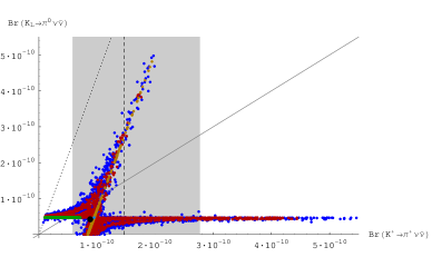
Figure 10: $Br(K_{\rm L}\rightarrow\pi^{0}\nu\bar{\nu})$ as a function of $Br(K^{+}\rightarrow\pi^{+}\nu\bar{\nu})$ in the LHT model. The shaded area represents the experimental $1\sigma$-range for $Br(K^{+}\rightarrow\pi^{+}\nu\bar{\nu})$. The GN-bound is displayed by the dotted line, while the solid line separates the two areas where $Br(K_{\rm L}\rightarrow\pi^{0}\nu\bar{\nu})$ is larger or smaller than $Br(K^{+}\rightarrow\pi^{+}\nu\bar{\nu})$.

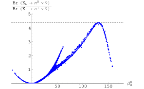
Figure 11: $Br(K_{\rm L}\rightarrow\pi^{0}\nu\bar{\nu})/Br(K^{+}\rightarrow\pi^{+}\nu\bar{\nu})$ in the LHT model as a function of $\beta_{X}^{K}$. The dashed line represents the GN-bound.

In Fig. 11 we show the ratio $Br(K_{\rm L}\rightarrow\pi^{0}\nu\bar{\nu})/Br(K^{+}\rightarrow\pi^{+}\nu\bar{\nu})$ as a function of the phase $\beta_{X}^{K}$, displaying again the GN-bound. We observe that the ratio can be significantly different from the SM prediction, with a possible enhancement of an order of magnitude.

The most interesting implications of this analysis are:

• If $Br(K^{+}\rightarrow\pi^{+}\nu\bar{\nu})$ is found sufficiently above the SM prediction but below $2.3\cdot 10^{-10}$, basically only two values for $Br(K_{\rm L}\rightarrow\pi^{0}\nu\bar{\nu})$ are possible within the LHT model. One of these values is very close to the SM value in (I.2) and the second much larger.

• If $Br(K^{+}\rightarrow\pi^{+}\nu\bar{\nu})$ is found above $2.3\cdot 10^{-10}$, then only $Br(K_{\rm L}\rightarrow\pi^{0}\nu\bar{\nu})$ with a value close to the SM one in (I.3) is possible.

• The violation of the MFV relation (I.1). We show this in Fig. 12, where the ratio of $\sin 2\beta_{X}^{K}$ over $\sin(2\beta+2\varphi_{B_{d}})$ is plotted versus $\delta^{d}_{13}$. As $\varphi_{B_{d}}$ is constrained by the measured $S_{\psi K_{S}}$ asymmetry to be at most a few degrees Blanke et al. (2006); Bona et al. (2006c), large violations of the relation in question can only follow from the $K\to\pi\nu\bar{\nu}$ decays. As seen in Fig. 12, they can be spectacular.

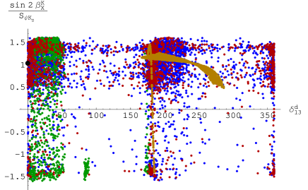
Figure 12: $\sin 2\beta_{X}^{K}/\sin(2\beta+2\varphi_{B_{d}})$ as a function of $\delta^{d}_{13}$ in the LHT model.

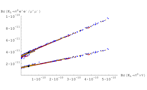
Figure 13: $Br(K_{L}\to\pi^{0}e^{+}e^{-})$ (upper curve) and $Br(K_{L}\to\pi^{0}\mu^{+}\mu^{-})$ (lower curve) as functions of $Br(K_{\rm L}\rightarrow\pi^{0}\nu\bar{\nu})$ in the LHT model. The corresponding SM predictions are represented by dark points.

Finally in Fig. 13 we show $Br(K_{L}\to\pi^{0}e^{+}e^{-})$ and $Br(K_{L}\to\pi^{0}\mu^{+}\mu^{-})$ versus $Br(K_{\rm L}\rightarrow\pi^{0}\nu\bar{\nu})$. We observe a strong correlation between $K_{L}\to\pi^{0}\ell^{+}\ell^{-}$ and $K_{\rm L}\rightarrow\pi^{0}\nu\bar{\nu}$ decays that we expect to be valid beyond the LHT model, at least in models with the same operators present as in the SM. We note that a large enhancement of $Br(K_{\rm L}\rightarrow\pi^{0}\nu\bar{\nu})$ automatically implies significant enhancements of $Br(K_{L}\to\pi^{0}\ell^{+}\ell^{-})$ and that different models and their parameter sets can than be distinguished by the position on the correlation curve. Moreover, measuring $Br(K_{L}\to\pi^{0}\ell^{+}\ell^{-})$ should allow a rather precise prediction of $Br(K_{\rm L}\rightarrow\pi^{0}\nu\bar{\nu})$ at least in models with the same operators as the SM. This should distinguish the LHT model from models with more complicated operator structure in $K_{L}\to\pi^{0}l^{+}l^{-}$ Mescia et al. (2006), and consequently different correlations between $K_{\rm L}\rightarrow\pi^{0}\nu\bar{\nu}$ and $K_{L}\to\pi^{0}l^{+}l^{-}$.

As emphasized in Buras and Silvestrini (1999); Buras et al. (2000), there exist correlations between $K\to\pi\nu\bar{\nu}$ decays, $K_{L}\to\mu^{+}\mu^{-}$ and $\varepsilon^{\prime}/\varepsilon$, that could bound the size of the enhancement of $Br(K^{+}\rightarrow\pi^{+}\nu\bar{\nu})$ and $Br(K_{\rm L}\rightarrow\pi^{0}\nu\bar{\nu})$. Unfortunately, the hadronic uncertainties in $K_{L}\to\mu^{+}\mu^{-}$ and in particular in $\varepsilon^{\prime}/\varepsilon$ lower the usefulness of these correlations at present. More promising, in the context of supersymmetric models and also generally, appear the correlations between $K\to\pi\nu\bar{\nu}$ and rare FCNC semileptonic decays like $B\to X_{s,d}l^{+}l^{-}$, $B_{s,d}\to l^{+}l^{-}$ and in particular $B\to X_{s,d}\nu\bar{\nu}$, because also in these decays the main deviations from the SM can be encoded in an effective $Z\bar{b}q$ ($q=s,d$) vertex Buchalla et al. (2001); Atwood and Hiller (2003). We have discussed the correlation with $B\to X_{s,d}\nu\bar{\nu}$ in the previous section.

Recently the correlation between $\epsilon^{\prime}/\epsilon$ and the decays $K\to\pi\nu\bar{\nu}$ has been investigated in the context of the LHT model for specific values of the relevant hadronic matrix elements entering $\epsilon^{\prime}/\epsilon$ Blanke et al. (2007b). The resulting correlation between $K_{\rm L}\rightarrow\pi^{0}\nu\bar{\nu}$ and $\epsilon^{\prime}/\epsilon$ is very strong but less pronounced in the case of $K^{+}\rightarrow\pi^{+}\nu\bar{\nu}$. With the hadronic matrix elements evaluated in the large-N limit, $(\epsilon^{\prime}/\epsilon)_{\rm SM}$ turns out to be close to the experimental data and significant departures of $Br(K_{\rm L}\rightarrow\pi^{0}\nu\bar{\nu})$ and $Br(K_{L}\to\pi^{0}l^{+}l^{-})$ from the SM expectations are unlikely, while $Br(K^{+}\rightarrow\pi^{+}\nu\bar{\nu})$ can be enhanced by a factor of 5. On the other hand, modest departures of the relevant hadronic matrix elements from their large-N values allow for a consistent description of $\epsilon^{\prime}/\epsilon$ within the LHT model accompanied by large enhancements of $Br(K_{\rm L}\rightarrow\pi^{0}\nu\bar{\nu})$ and $Br(K_{L}\to\pi^{0}l^{+}l^{-})$, but only modest enhancements of $Br(K^{+}\rightarrow\pi^{+}\nu\bar{\nu})$. This analysis demonstrates very clearly that without a significant progress in the evaluation of the hadronic parameters in $\epsilon^{\prime}/\epsilon$, the role of this ratio in constraining physics beyond the SM will remain limited.

VIII.3 $Z^{\prime}$ Models

An additional neutral gauge boson can appear in several extensions of the standard model, such as Left-Right Symmetric Models, SUSY models with an additional $U(1)$ Factor, often arising in the breaking process of several GUT models, such as the breaking chain $SO(10)\to SU(5)\times U(1)$ or $E_{6}\to SO(10)\times U(1)$, or in 331 models, where the $SU(2)_{L}$ of the SM is extended to an $SU(3)_{L}$. In general, direct collider searches have already placed some lower bounds on a general $Z^{\prime}$ mass, but FCNC processes can also provide valuable information on these particles, since additional contributions appear at tree level, if the $Z^{\prime}$ transmits flavour changes. General, model independent, analyses of $B$ decays as well as the mass differences $\Delta M_{s}$ can be found in Langacker and Plumacher (2000); Grossman et al. (1999); Barger et al. (2004b, a). Additional interest in these contributions with respect to the $B$ meson system has arisen in the context of the CP asymmetries in $B^{0}_{d}\to\phi K_{S}$. In general, one finds that sizeable contributions are still well possible but are rather unpredictive in this model independent context. On the other hand, predictive power increases if the analysis is performed in a specific model.

As an example for this situation, we discuss the recent analysis Promberger et al. (2007) performed in the minimal 331 model Frampton (1992); Pisano and Pleitez (1992). Here, one has an $SU(3)_{c}\times SU(3)_{L}\times U(1)$ which is broken down to the electromagnetic $U(1)$ in two steps. In this process, the additional $Z^{\prime}$ boson appears, along with several charged gauge bosons, that play no role in low energy processes involving quarks, since they always couple to the additional heavy quarks that fill the left-handed triplet. Finally, the third generation of quarks is treated differently from the first two, transforming as an anti-triplet. In this setup, taking into account also the asymptotic freedom of QCD, one finds that anomalies are canceled precisely in the case of the three generations, thereby explaining this feature of the SM, where the numbers of generations is fixed from observation. Apart from FCNC processes, constraints on the $Z^{\prime}$ mass come also from electroweak precision observables, but the new contributions here appear at the one loop level, so that the constraints from FCNCs are actually more interesting. Also, the model develops a Landau pole at a scale of several $\mathrm{TeV}$, which constrains the new energy scale from above, thereby complementing the bounds from direct searches and FCNC observables.

The flavour non-universality reflected in the different transformation property of the third generation leads to the flavour changing $Z^{\prime}$ vertices. The FCNC processes under investigation then depend on the $Z^{\prime}$ mass as well as the weak mixing matrix required to diagonalize the Yukawa coupling of the down quark sector (as long as one is studying $B$ or $K$ meson processes). Also, one finds that the different processes decouple from each other, i.e. that $sd$, $bd$ and $bs$ transitions are constrained independently, so that only the constraints from $\Delta M_{K}$ and $\varepsilon_{K}$ are used to constrain the branching fractions of $K_{\rm L}\rightarrow\pi^{0}\nu\bar{\nu}$ and $K^{+}\rightarrow\pi^{+}\nu\bar{\nu}$. This leads to an allowed region in the $K_{\rm L}\rightarrow\pi^{0}\nu\bar{\nu}-K^{+}\rightarrow\pi^{+}\nu\bar{\nu}$ plane shown in Fig. 14. We show the corresponding areas for $M_{Z^{\prime}}=1~{}\mathrm{TeV}$ as well as $M_{Z^{\prime}}=5~{}\mathrm{TeV}$, where one observes that the allowed region shrinks with increasing $M_{Z^{\prime}}$. The pattern is similar to the one shown in the LHT model, in that there exist two possible branches, where $Br(K_{\rm L}\rightarrow\pi^{0}\nu\bar{\nu})$ is close to the SM on one of them, while $Br(K^{+}\rightarrow\pi^{+}\nu\bar{\nu})$ is on the other. This is due to the different strength of the $\varepsilon_{K}$ and $\Delta M_{K}$ bounds, respectively, and the large modifications arise in those areas, where the phase of the new contribution is such, that it does not modify $\varepsilon_{K}$ strongly. Therefore a similar structure should appear whenever the $K\to\pi^{0}\nu\bar{\nu}$ decays are constrained mainly by these two quantities. On the other hand, the minimal 331 model has a somewhat leptophobic nature, so that the effects are not expected to be as large as, for example, in the LHT model, but the current experimental central value can be reached, in particular for $M_{Z^{\prime}}<2\mathrm{TeV}$.

Additionally, a measurement of both branching fractions fixes both the absolute value and phase of the new contributions (this is true in all $Z^{\prime}$ models) and allows predictions for the observables $\Delta M_{K}$ and $\varepsilon_{K}$ (this is of course only true if the model is explicitely fixed). Another interesting feature of this model is that there are significant differences between the vector and axial vector coupling, which cancel each other out in the $V-A$ difference, to which $Br(K_{\rm L}\rightarrow\pi^{0}\nu\bar{\nu})$ is sensitive, so that, in comparison, one finds stronger modifications in the $K_{L}\to\pi^{0}l^{+}l^{-}$ branching fraction than in $K_{\rm L}\rightarrow\pi^{0}\nu\bar{\nu}$ Promberger et al. (2007). Finally, significant modifications can also be found in the angle $\beta|_{K\pi\nu\nu}$, which may be as large as $45^{\circ}$ for small values of $M_{Z^{\prime}}$.

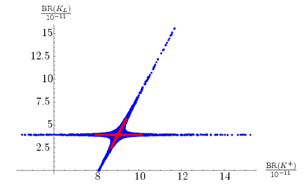
Figure 14: A projection onto the $K_{\rm L}\rightarrow\pi^{0}\nu\bar{\nu}$-$K^{+}\rightarrow\pi^{+}\nu\bar{\nu}$ plane including the upper bounds from $\Delta M_{K}$ and $\epsilon_{K}$ for $M_{Z^{\prime}}=5~{}\mathrm{TeV}$ (red) and $M_{Z^{\prime}}=1~{}\mathrm{TeV}$ (blue).

On the other hand, recently He and Valencia (2004, 2006) the decays $K\to\pi\nu\bar{\nu}$ have been analyzed in models that are variations of left-right symmetric models in which right-handed interactions, involving in particular a heavy $Z^{\prime}$ boson, single out the third generation He and Valencia (2002, 2003). The contributions of these new non-universal FCNC interactions appear both at the tree and one-loop level. The tree level contributions involving $Z^{\prime}$ of the type $(\bar{s}d)_{V+A}(\bar{\nu}_{\tau}\nu_{\tau})_{V+A}$ can be severely constrained by other rare decays, $\varepsilon_{K}$ and in particular $B^{0}_{s}-\bar{B}^{0}_{s}$ mixing. Before the measurement of $\Delta M_{s}$, these could enhance $Br(K^{+}\rightarrow\pi^{+}\nu\bar{\nu})$ to the central experimental value in (I.5) and $Br(K_{\rm L}\rightarrow\pi^{0}\nu\bar{\nu})$ could be as high as $1.4\cdot 10^{-10}$. These enhancements where accompanied by an enhancement of $\Delta M_{s}$ and finding $\Delta M_{s}$ in the ball park of the SM expectations has significantly limited these possibilities He and Valencia (2006). On the other hand new one loop contributions involving $Z^{\prime}$ boson may be important, because of the particularly large $\tau$ neutrino coupling. They are not constrained by $B^{0}_{s}-\bar{B}^{0}_{s}$ mixing and can give significant enhancements of both branching ratios even if $\Delta M_{s}\approx(\Delta M_{s})_{SM}$. Unfortunately the presence of many free parameters in these new one-loop contributions does not allow to make definite predictions, but an enhancement by a factor of two still seems possible He and Valencia (2006).

Finally, FCNC processes at tree level arise also if there is an additional vector-like quark generation, or, if there is only one additional isosinglet down-type or up-type quark, as one can encounter in certain $E_{6}$ GUT theories, or some models with extra dimensions. In this case, the SM $Z$ itself boson can transmit flavor changes, since the mixing matrix of the respective quark sector is no longer unitary and therefore does not cancel out in the neutral $Z$-current, causing FCNCs in the respective sector where the additional quark appears. The most recent analysis of the $K\to\pi\nu\bar{\nu}$ decays in this model has been presented in Deshpande et al. (2004), while a very complete analysis of FCNC processes in this type of scenario can be found in Barenboim et al. (2001). Here, the authors obtain constraints on the matrix element $U_{sd}$ (here $U=V^{\dagger}V$, with $V$ being the mixing matrix that diagonalizes the down quark sector) from $K^{+}\rightarrow\pi^{+}\nu\bar{\nu}$, $\varepsilon_{K}$, $\varepsilon^{\prime}/\varepsilon_{K}$. Additionally, they emphasize that the $K\to\pi\nu\bar{\nu}$ decays can be very valuable for constraining this element further, if the decays are precisely measured. In fact, one finds there a figure somewhat similar in spirit to the one shown in Fig. 14, which shows an analogous interplay of constraints in the $K$ physics sector. We have included this figure as Fig. 15.

Figure 15: Effect of the constraints from $\varepsilon_{K}$, $K^{+}\rightarrow\pi^{+}\nu\bar{\nu}$, $K_{L}\rightarrow\mu^{+}\mu^{-}$ and $\varepsilon^{\prime}/\varepsilon$ on the $U_{sd}$ FCNC coupling in case of an extra isosinglet down quark Barenboim et al. (2001).

VIII.4 MSSM with MFV

There are many new contributions in MSSM such as charged Higgs, chargino, neutralino and gluino contributions. However, in the case of $K\to\pi\nu\bar{\nu}$ and MFV it is a good approximation to keep only charged Higgs and chargino contributions.

To our knowledge the first analyses of $K\to\pi\nu\bar{\nu}$ in this scenario can be found in Bertolini and Masiero (1986); Giudice (1987); Mukhopadhyaya and Raychaudhuri (1987); Bigi and Gabbiani (1991), subsequently in Couture and Konig (1995); Goto et al. (1998) and in Buras et al. (2001a). In the latter analysis constraints on the supersymmetric parameters from $\varepsilon_{K}$, $\Delta M_{d,s}$, $B\to X_{s}\gamma$, $\Delta\varrho$ in the electroweak precision studies and from the lower bound on the neutral Higgs mass have been imposed. Supersymmetric contributions affect both the loop functions like $X(v)$ present in the SM and the values of the extracted CKM parameters like $|V_{td}|$ and ${\rm Im}\lambda_{t}$. As the supersymmetric contributions to the function $S(v)$ relevant for the analysis of the UT are always positive (see also Altmannshofer et al. (2007)), the extracted values of $|V_{td}|$ and ${\rm Im}\lambda_{t}$ are always smaller than in the SM. Consequently, $Br(K^{+}\rightarrow\pi^{+}\nu\bar{\nu})$ and $Br(K_{\rm L}\rightarrow\pi^{0}\nu\bar{\nu})$, that are sensitive to $|V_{td}|$ and ${\rm Im}\lambda_{t}$, respectively, are generally suppressed relative to the SM expectations. The supersymmetric contributions to the loop function $X(v)$ can compensate the suppression of $|V_{td}|$ and ${\rm Im}\lambda_{t}$ only for special values of supersymmetric parameters, so that in these cases the results are very close to the SM expectations.

Setting $\lambda$, $|V_{ub}|$ and $|V_{cb}|$, all unaffected by SUSY contributions, at their central values one finds Buras et al. (2001a)

$$0.65\leq\frac{Br(K^{+}\rightarrow\pi^{+}\nu\bar{\nu})}{Br(K^{+}\rightarrow\pi^{+}\nu\bar{\nu})_{\rm SM}}\leq 1.02,\qquad 0.41\leq\frac{Br(K_{\rm L}\rightarrow\pi^{0}\nu\bar{\nu})}{Br(K_{\rm L}\rightarrow\pi^{0}\nu\bar{\nu})_{\rm SM}}\leq 1.03.$$ (VIII.29)

We observe that significant suppressions of the branching ratios relative to the SM expectations are still possible. More importantly, finding experimentally at least one of these branching ratios above the SM value would exclude this scenario, indicating new flavour violating sources beyond the CKM matrix. Similarly, in the MSSM based on supergravity a reduction of both $K\to\pi\nu\bar{\nu}$ rates up to $10\%$ is possible Goto et al. (1998).

Reference Buras et al. (2001a) provides a compendium of phenomenologically relevant formulae in the MSSM, that should turn out to be useful once the relevant branching ratios have been accurately measured and the supersymmetric particles have been discovered at Tevatron, LHC and the $e^{+}e^{-}$ linear collider. The study of the unitarity triangle can be found in Ali and London (1999c, b, a, 2001). The inclusion of NLO QCD corrections to the processes discussed in Buras et al. (2001a) has been performed in Bobeth et al. (2002). These corrections reduce mainly the renormalization scale uncertainties present in the analysis of Buras et al. (2001a), without modifying the results in (VIII.29) significantly.

VIII.5 General Supersymmetric Models

In general supersymmetric models the effects of supersymmetric contributions to rare branching ratios can be larger than discussed above. In these models new CP-violating phases and new operators are present. Moreover the structure of flavour violating interactions is much richer than in the MFV models.

The new flavour violating interactions are present because generally the sfermion mass matrices $\tilde{M}_{q}^{2}$ can be non-diagonal in the basis in which all neutral quark-squark-gaugino vertices and quark and lepton mass matrices are flavour diagonal. Instead of diagonalizing sfermion mass matrices it is convenient to consider their off-diagonal terms as new flavour violating interactions. This so–called mass–insertion approximation Hall et al. (1986) has been reviewed in the classic papers Gabbiani et al. (1996); Misiak et al. (1998), where further references can be found.

Within the MSSM with $R$-parity conservation, sizable non-standard contributions to $K\to\pi\nu\overline{\nu}$ decays can be generated if the soft-breaking terms have a non-MFV structure. The leading amplitudes giving rise to large effects are induced by: i) chargino/up-squark loops Nir and Worah (1998); Buras et al. (1998); Colangelo and Isidori (1998); Buras et al. (2000) ii) charged Higgs/top quark loops Isidori and Paradisi (2006). In the first case, large effects are generated if the left-right mixing ($A$ term) of the up-squarks has a non-MFV structure D’Ambrosio et al. (2002). In the second case, deviations from the SM are induced by non-MFV terms in the right-right down sector, provided the ratio of the two Higgs vacuum expectation values ($\tan\beta=v_{u}/v_{d}$) is large ($\tan\beta\sim 30-50$).

The effective Hamiltonian encoding SD contributions in the general MSSM has the following structure:

$${\mathcal{H}}_{\rm eff}^{(\rm SD)}\propto\sum_{l=e,\mu,\tau}V^{\ast}_{ts}V_{td}\left[X_{L}(\bar{s}_{L}\gamma^{\mu}d_{L})(\bar{\nu}_{lL}\gamma_{\mu}\nu_{lL})+X_{R}(\bar{s}_{R}\gamma^{\mu}d_{R})(\bar{\nu}_{lL}\gamma_{\mu}\nu_{lL})\right]~{},$$ (VIII.30)

where the SM case is recovered for ${X_{R}=0}$ and $X_{L}=X_{\rm SM}$. In general, both $X_{R}$ and $X_{L}$ are non-vanishing, and the misalignment between quark and squark flavour structures implies that they are both complex quantities. Since the $K\to\pi$ matrix elements of $(\bar{s}_{L}\gamma^{\mu}d_{L})$ and $(\bar{s}_{R}\gamma^{\mu}d_{R})$ are equal, the combination $X_{L}+X_{R}$ allows us to describe all the SD contributions to $K\to\pi\nu\overline{\nu}$ decays. More precisely, we can simply use the SM expressions for the branching ratios with the following replacement

$$X_{\rm SM}\to X_{\rm SM}+X^{\rm SUSY}_{L}+X^{\rm SUSY}_{R}~{},$$ (VIII.31)

with $X_{L,R}^{\rm SUSY}$ being complex quantities. In the limit of almost degenerate superpartners, the leading chargino/up-squarks contribution is Colangelo and Isidori (1998):

$$X^{\chi^{\pm}}_{L}\approx\frac{1}{96}\left[\frac{(\delta^{u}_{LR})_{23}(\delta^{u}_{RL})_{31}}{\lambda_{t}}\right]~{}=~{}\frac{1}{96\lambda_{t}}\left[\frac{(\tilde{M}^{2}_{u})_{2_{L}3_{R}}}{(\tilde{M}^{2}_{u})_{LL}(\tilde{M}^{2}_{u})_{RR}}\right]\left[\frac{(\tilde{M}^{2}_{u})_{3_{R}1_{L}}}{(\tilde{M}^{2}_{u})_{LL}(\tilde{M}^{2}_{u})_{RR}}\right]\,.$$ (VIII.32)

Here $(\delta_{AB}^{q})_{ij}$ result from a convenient parametrization Gabbiani et al. (1996); Misiak et al. (1998) of the non-diagonal terms $(\tilde{M}_{u}^{2})_{iAjB}$ in squark mass matrices with $A,B=L,R$ and $i,j=1,2,3$ standing for quark generation indices. As pointed out in Colangelo and Isidori (1998), a remarkable feature of the above result is that no extra $\mathcal{O}(M_{W}/M_{\rm SUSY})$ suppression and no explicit CKM suppression is present (as it happens in the chargino/up-squark contributions to other processes). Furthermore, the $(\delta^{u}_{LR})$-type mass insertions are not strongly constrained by other $B$- and $K$-observables. This implies that large departures from the SM expectations in $K\to\pi\nu\overline{\nu}$ decays are allowed, as confirmed by the complete analyses in Buras et al. (2005a); Isidori et al. (2006b). In particular in Buras et al. (2005a) one finds that both branching ratios can be as large as few times $10^{-10}$ with $Br(K_{\rm L}\rightarrow\pi^{0}\nu\bar{\nu})$ often larger than $Br(K^{+}\rightarrow\pi^{+}\nu\bar{\nu})$ and close to the GN bound. One also finds Isidori et al. (2006b) that $K\to\pi\nu\overline{\nu}$ are the best observables to determine/constrain from experimental data the size of the off-diagonal $(\delta^{u}_{LR})$ mass insertions or, equivalently, the up-type trilinear terms $A_{i3}$ [$(\tilde{M}^{2}_{u})_{i_{L}3_{R}}\approx m_{t}A_{i3}$]. Their measurement is therefore extremely interesting also in the LHC era.

In the large $\tan\beta$ limit, the charged Higgs/ top quark exchange leads to Isidori and Paradisi (2006):

$$X^{H^{\pm}}_{R}\approx\left[\left(\frac{m_{s}m_{d}\,t^{2}_{\beta}}{2M_{W}^{2}}\right)+\frac{(\delta^{d}_{RR})_{31}(\delta^{d}_{RR})_{32}}{\lambda_{t}}\left(\frac{m^{2}_{b}\,t^{2}_{\beta}}{2M_{W}^{2}}\right)\frac{\epsilon^{2}_{RR}t^{2}_{\beta}}{(1+\epsilon_{i}t_{\beta})^{4}}\right]f_{H}(y_{tH})\,,$$ (VIII.33)

where $y_{tH}=m_{t}^{2}/M_{H}^{2}$, $f_{H}(x)=x/4(1-x)+x\log x/4(x-1)^{2}$ and $\epsilon_{i,RR}t_{\beta}=\mathcal{O}(1)$ for $t_{\beta}=\tan\beta\sim 50$. The first term of Eq. (VIII.33) arises from MFV effects and its potential $\tan\beta$ enhancement is more than compensated by the smallness of $m_{d,s}$. The second term on the r.h.s. of Eq. (VIII.33), which would appear only at the three-loop level in a standard loop expansion can be largely enhanced by the $\tan^{4}\beta$ factor and does not contain any suppression due to light quark masses. Similarly to the double mass-insertion mechanism of Eq. (VIII.32), also in this case the potentially leading effect is the one generated when two off-diagonal squark mixing terms replace the two CKM factors $V_{ts}$ and $V_{td}$.

The coupling of the $(\bar{s}_{R}\gamma^{\mu}d_{R})(\bar{\nu}_{L}\gamma_{\mu}\nu_{L})$ effective FCNC operator, generated by charged-Higgs/top quark loops is phenomenologically relevant only at large $\tan\beta$ and with non-MFV right-right soft-breaking terms: a specific but well-motivated scenario within grand-unified theories (see e.g. Moroi (2000); Chang et al. (2003)). These non-standard effects do not vanish in the limit of heavy squarks and gauginos, and have a slow decoupling with respect to the charged-Higgs boson mass. As shown in Isidori and Paradisi (2006) the $B$-physics constraints still allow a large room of non-standard effects in $K\to\pi\nu\overline{\nu}$ even for flavour-mixing terms of CKM size (see Fig. 16).

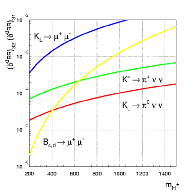
Figure 16: Supersymmetric contributions to $K\to\pi\nu\bar{\nu}$. Sensitivity to $(\delta^{d}_{RR})_{23}(\delta^{d}_{RR})_{31}$ of various rare $K$- and $B$-decays as a function of $M_{H^{+}}$, setting $\tan\beta\!=\!50$, $\mu\!<\!0$ and assuming almost degenerate superparteners (the bounds from the two $K\rightarrow\pi\nu\bar{\nu}$ modes are obtained assuming a $10\%$ measurement of their branching ratios while the $B_{s,d}\rightarrow\mu^{+}\mu^{-}$ bounds refer to the present experimental limits Isidori and Paradisi (2006)).

A systematic study of $K\to\pi\nu\bar{\nu}$ decays in flavour supersymmetric models has been performed in Nir and Worah (1998); Nir and Raz (2002). These particular models are designed to solve naturally the CP and flavour problems characteristic for supersymmetric theories. They are more constrained than the general supersymmetric models just discussed, in which parameters are tuned to satisfy the experimental constraints.

Models with exact universality of squark masses at a high energy scale with the $A$ terms proportional to the corresponding Yukawa couplings, models with approximate CP, quark and squark alignment, approximate universality and heavy squarks have been analyzed in Nir and Worah (1998); Nir and Raz (2002) in general terms. It has been concluded that in most of these models the impact of new physics on $K\to\pi\nu\bar{\nu}$ is sufficiently small so that in these scenarios one can get information on the CKM matrix from these decays even in the presence of supersymmetry. On the other hand, supersymmetric contributions to $B^{0}_{d}-\bar{B}^{0}_{d}$ mixing in models with alignment, with approximate universality and heavy squarks can significantly affect the asymmetry $a_{\psi K_{S}}$, so that in these models the golden relation (I.1) can be violated. However such scenarios have been put under large pressure in view of the recent data on $D^{0}-\bar{D}^{0}$ mixing Nir (2007); Ciuchini et al. (0300).

Finally, in supersymmetric models with non-universal $A$ terms, enhancements of $Br(K^{+}\rightarrow\pi^{+}\nu\bar{\nu})$ and $Br(K_{\rm L}\rightarrow\pi^{0}\nu\bar{\nu})$ up to $1.5\cdot 10^{-10}$ and $2.5\cdot 10^{-10}$ are possible, respectively Chen (2002). Significant departures from the SM expectations have also been found in supersymmetric models with R-parity breaking Deandrea et al. (2004), but all these analyses should be reconsidered in view of experimental constraints.

VIII.6 Models with Universal Extra Dimensions

The decays $K^{+}\rightarrow\pi^{+}\nu\bar{\nu}$ and $K_{\rm L}\rightarrow\pi^{0}\nu\bar{\nu}$ have been studied in the SM model with one extra universal dimension in Buras et al. (2003b). In this model (ACD) Appelquist et al. (2001) all the SM fields are allowed to propagate in all available dimensions and the relevant penguin and box diagrams receive additional contributions from Kaluza-Klein (KK) modes. This model belongs to the class of CMFV models and the only additional free parameter relative to the SM is the compactification scale $1/R$. Extensive analyses of the precision electroweak data, the analyses of the anomalous magnetic moment of the muon and of the $Z\to b\bar{b}$ vertex have shown the consistency of the ACD model with the data for $1/R\geq 300\,{\rm GeV}$. We refer to Buras et al. (2003b, 2004c) for the list of relevant papers.

For $1/R=300\,{\rm GeV}$ and $1/R=400\,{\rm GeV}$ the function $X$ is found with $m_{t}=167\,{\rm GeV}$ to be $X=1.67$ and $X=1.61$, respectively. This should be compared with $X=1.53$ in the SM. In contrast to the analysis in the MSSM discussed in Buras et al. (2001a) and above, this $5-10\%$ enhancement of the function $X$ is only insignificantly compensated by the change in the values of the CKM parameters. Consequently, the clear prediction of the model are the enhanced branching ratios $Br(K^{+}\rightarrow\pi^{+}\nu\bar{\nu})$ and $Br(K_{\rm L}\rightarrow\pi^{0}\nu\bar{\nu})$, albeit by at most $15\%$ relative to the SM expectation. These enhancements allow to distinguish this scenario from the MSSM with MFV.

The enhancement of $Br(K^{+}\rightarrow\pi^{+}\nu\bar{\nu})$ in the ACD model is interesting in view of the experimental results in (I.5) with the central value by a factor of $1.8$ higher than the central value in the SM. Even if the errors are substantial and this result is compatible with the SM, the ACD model with a low compactification scale is closer to the data. In table 12 we show the upper bound on $Br(K^{+}\rightarrow\pi^{+}\nu\bar{\nu})$ in the ACD model obtained in Buras et al. (2003b) by means of the formula (III.10), with $X$ replaced by its enhanced value in the model in question. To this end $|V_{cb}|\leq 0.0422$, $P_{c}(X)<0.47$, $m_{\rm t}(m_{t})<172~{}\,{\rm GeV}$ and $\sin 2\beta=0.734$ have been used. Table 12 illustrates the dependence of the bound on the nonperturbative parameter $\xi$, $1/R$ and $\Delta M_{s}$. We observe that for $1/R=300~{}\,{\rm GeV}$ and $\xi=1.30$ the maximal value for $Br(K^{+}\rightarrow\pi^{+}\nu\bar{\nu})$ in the ACD model is rather close to the central value in (I.5).

Table 12: Upper bound on $Br(K^{+}\rightarrow\pi^{+}\nu\bar{\nu})$ in units of $10^{-11}$ for different values of $\xi$, $1/R$ and $\Delta M_{s}=18/{\rm ps}~{}(21/{\rm ps})$ from Buras et al. (2003b).

$\xi$	$1/R=300~{}\,{\rm GeV}$	$1/R=400~{}\,{\rm GeV}$	SM
$1.30$	$12.0~{}(10.7)$	$11.3~{}(10.1)$	$10.8~{}(9.3)$
$1.25$	$11.4~{}(10.2)$	$10.7~{}(9.6)$	$10.3~{}(8.8)$
$1.20$	$10.7~{}(9.6)$	$10.1~{}(9.1)$	$9.7~{}(8.4)$
$1.15$	$10.1~{}(9.0)$	$9.5~{}(8.5)$	$9.1~{}(7.9)$

Clearly, in order to distinguish these results and the ACD model from the SM, other quantities, that are more sensitive to $1/R$, should be simultaneously considered. In this respect, the sizable downward shift of the zero ($\hat{s}_{0}$) in the forward-backward asymmetry $A_{\rm FB}$ in $B\to X_{s}\mu^{+}\mu^{-}$ and the suppression of $Br(B\to X_{s}\gamma)$ by roughly $20\%$ at $1/R=300\,{\rm GeV}$ appear to be most interesting Buras et al. (2004c).

As the most recent analysis of the $B\to X_{s}\gamma$ decay at the NNLO level results in its SM branching ratio being by more than one $\sigma$ below the experimental values, the model in question is put therefore under considerable pressure and the values of $1/R$ as low as 300 GeV appear rather improbable from the present perspective Haisch and Weiler (0300). A decrease of the experimental error without a significant change of its central value and a better understanding of non-perturbative effects in the $B\to X_{s}\gamma$ decay could result in $1/R\approx{\cal O}(1{\rm TeV})$ and consequently very small new physics effects in $K\to\pi\nu\bar{\nu}$ decays in this model.

VIII.7 Models with Lepton-Flavour Mixing

In the presence of flavour mixing in the leptonic sector, the transition $K_{L}\to\pi^{0}\nu_{i}\bar{\nu}_{j}$, with $i\not=j$ could receive significant CP-conserving contributions Grossman and Nir (1997). Subsequently this issue has been analyzed in Perez (1999, 2000) and in Grossman et al. (2004). Here we summarize briefly the main findings of these papers.

In Perez (1999, 2000) the effect of light sterile right-handed neutrinos leading to scalar and tensor dimension-six operators has been analyzed. As shown there, the effect of these operators is negligible, if the right-handed neutrinos interact with the SM fields only through their Dirac mass terms.

Larger effects are expected from the operators

$$O^{ij}_{sd}=(\bar{s}\gamma_{\mu}d)(\bar{\nu}^{i}_{L}\gamma^{\mu}\nu^{j}_{L}),$$ (VIII.34)

that for $(i\not=j)$ create a neutrino pair which is not a CP eigenstate. As shown in Grossman et al. (2004) the condition for a non-vanishing $K_{\rm L}\rightarrow\pi^{0}\nu\bar{\nu}$ rate in this case is rather strong. One needs either CP violation in the quark sector or a new effective interaction that violates both quark and lepton universality. One finds then the following pattern of effects:

• If the source of universality breaking is confined to mass matrices, the effects of lepton-flavour mixing get washed out in the $K\to\pi\nu\bar{\nu}$ rates after the sum over the neutrino flavours has been done. There are in principle detectable effects of lepton mixing only in cases where there are two different lepton-flavour mixing matrices, although they cannot be large.

• In models in which simultaneous violation of quark and lepton universality proceeds entirely through Yukawa couplings, the CP conserving effects in $K\to\pi\nu\bar{\nu}$ are suppressed by Yukawa couplings. As explicitly shown in Grossman et al. (2004) even in the MSSM with flavour violation and large $\tan\beta$ these types of effects are negligible.

• In exotic scenarios, such as R-parity violating supersymmetric models, lepton flavour mixing could generate sizable CP-conserving contributions to $K_{\rm L}\rightarrow\pi^{0}\nu\bar{\nu}$ and generally in $K\to\pi\nu\bar{\nu}$ rates.

VIII.8 Other Models

There exist other numerous analyses of $K\to\pi\nu\bar{\nu}$ decays within various extensions of the SM. For completeness we briefly describe them here.

In Carlson et al. (1996) the rate for $K_{\rm L}\rightarrow\pi^{0}\nu\bar{\nu}$ has been calculated in several extensions of the SM Higgs sector, including the Liu-Wolfenstein two-doublet model of spontaneous CP- violation and the Weinberg three doublet model. It has been concluded that although in the usual two Higgs doublet model, with CP-violation governed by the CKM matrix, some measurable effects could be seen, in models in which CP-violation arises either entirely or predominantly from the Higgs sector the decay rate is much smaller than in the SM.

The study of $K\to\pi\nu\bar{\nu}$ in models with four generations, extra vector-like quarks and isosinglet down quarks can be found in Huang et al. (2001); Hung and Soddu (2002); Hawkins and Silverman (2002); Yanir (2002); Aguilar-Saavedra (2003); Hattori et al. (1998). In particular in four generation models Huang et al. (2001); Yanir (2002); Hattori et al. (1998) due to three additional mixing angles and two additional complex phases, $Br(K_{\rm L}\rightarrow\pi^{0}\nu\bar{\nu})$ can be enhanced by 1-2 orders of magnitude with respect to the SM expectations and also $Br(K^{+}\rightarrow\pi^{+}\nu\bar{\nu})$ can be significantly enhanced. Unfortunately, due to many free parameters, the four generation models are not very predictive. A new analysis of $K\to\pi\nu\bar{\nu}$ in a model with an extra isosinglet down quark appeared in Deshpande et al. (2004). Putting all the available constraints on the parameters of this model, the authors conclude that $Br(K^{+}\rightarrow\pi^{+}\nu\bar{\nu})$ can still be enhanced up to the present experimental central value, while $Br(K_{\rm L}\rightarrow\pi^{0}\nu\bar{\nu})$ can reach $1\cdot 10^{-10}$.

The decays $K\to\pi\nu\bar{\nu}$ have also been investigated in a seesaw model for quark masses Kiyo et al. (1999). In this model there are scalar operators $(\bar{s}d)(\bar{\nu}_{\tau}\nu_{\tau})$, resulting from LR box diagrams, that make the rate for $K_{\rm L}\rightarrow\pi^{0}\nu\bar{\nu}$ non-vanishing even in the CP conserving limit and in the absence of lepton-flavour mixing. But the enhancement of $Br(K_{\rm L}\rightarrow\pi^{0}\nu\bar{\nu})$ due to these operators is at most of order $30\%$ even for $M_{W_{R}}=500\,{\rm GeV}$ with a smaller effect in $Br(K^{+}\rightarrow\pi^{+}\nu\bar{\nu})$.

The effects of the electroweak symmetry breaking on rare $K$ and $B$ decays, including $K\to\pi\nu\bar{\nu}$, in the presence of new strong dynamics, have been worked out in Buchalla et al. (1996b); Burdman (1997). Deviations from the SM in $K\to\pi\nu\bar{\nu}$ have been shown to be correlated with the ones in $B$ decays Burdman (1997).

The implications of a modified effective $Zb\bar{b}$ vertex on $K\to\pi\nu\bar{\nu}$, in connection with the small disagreement between the SM and the measured asymmetry $A^{b}_{FB}$ at LEP, have been discussed in Chanowitz (2001, 1999). While the predictions are rather uncertain, an enhancement of $Br(K^{+}\rightarrow\pi^{+}\nu\bar{\nu})$ by a factor of two, towards the central experimental value, is possible.

Enhancement of both $K\to\pi\nu\bar{\nu}$ branching ratios up to $50\%$ has been found in a five dimensional split fermions scenario Chang and Ng (2002) and the decay $K^{+}\rightarrow\pi^{+}\nu\bar{\nu}$ turns out to be the best for providing the constraints on the bulk SM in the Randall-Sundrum scenario Burdman (2002).

VIII.9 Summary

We have seen in this and the previous section that many scenarios of new physics allow still for significant enhancements of both $Br(K^{+}\rightarrow\pi^{+}\nu\bar{\nu})$ and $Br(K_{\rm L}\rightarrow\pi^{0}\nu\bar{\nu})$: $Br(K^{+}\rightarrow\pi^{+}\nu\bar{\nu})$ can still be enhanced by factors of 2-3 and $Br(K_{\rm L}\rightarrow\pi^{0}\nu\bar{\nu})$ could be by an order of magnitude larger than expected within the SM. While for obvious reasons most of the papers concentrate on possible enhancements of both branching ratios, their suppressions in several scenarios are still possible. This is in particular the case of the MSSM with MFV and in several models in which CP violation arises from the Higgs sector.

Because most models contain several free parameters, definite predictions for $K\to\pi\nu\bar{\nu}$ can only be achieved by considering simultaneously as many processes as possible so that these parameters are sufficiently constrained.

IX Comparison with Other Decays

After this exposition of $K^{+}\rightarrow\pi^{+}\nu\bar{\nu}$ and $K_{\rm L}\rightarrow\pi^{0}\nu\bar{\nu}$ decays in the SM and its most studied extensions we would like to briefly compare the potential of these two clean rare decays in extracting the CKM parameters and in testing the SM and its extensions with other prominent $K$ and $B$ decays for which a rich literature exists. A subset of relevant references will be given below.

In the $K$ system, the most investigated in the past are the parameters $\varepsilon_{K}$ and the ratio $\varepsilon^{\prime}/\varepsilon$ that describe respectively the indirect and direct CP violation in $K_{L}\to\pi\pi$ decays and the rare decays $K_{L}\to\mu^{+}\mu^{-}$ and $K_{L}\to\pi^{0}e^{+}e^{-}$. None of them can compete in the theoretical cleanness with the decays considered here but some of them are still useful.

While $K_{L}\to\mu^{+}\mu^{-}$ and $\varepsilon^{\prime}/\varepsilon$ suffer from large hadronic uncertainties, the case of the decays $K_{L}\to\pi^{0}\mu^{+}\mu^{-}$ and $K_{L}\to\pi^{0}e^{+}e^{-}$ is much more promising. They provide an interesting and complementary window to $|\Delta S|=1$ SD transitions. While the latter is theoretically not as clean as the $K\to\pi\nu\bar{\nu}$ system, it is sensitive to different types of SD operators. The $K_{L}\to\pi^{0}\ell^{+}\ell^{-}$ decay amplitudes have three main ingredients: i) a clean direct-CP-Violating (CPV) component determined by SD dynamics; ii) an indirect-CPV term due to $K^{0}$–$\overline{K^{0}}$ mixing; iii) a LD CP-Conserving (CPC) component due to two-photon intermediate states. Although generated by very different dynamics, these three components are of comparable size and can be computed (or indirectly determined) to good accuracy within the SM Buchalla et al. (2003); Isidori et al. (2004). In the presence of non-vanishing NP contributions, the combined measurements of $K\to\pi\nu\bar{\nu}$ and $K_{L}\to\pi^{0}\ell^{+}\ell^{-}$ decays provide a unique tool to distinguish among different NP models.

Most advanced analyses of these decays within the SM can be found in Buchalla et al. (2003); Isidori et al. (2004); Friot et al. (2004), where further references to earlier literature can be found. We would like also to mention the recent analyses of these decays in the context of the MSSM Isidori et al. (2006b) and other NP scenarios Mescia et al. (2006), in particular in the LHT model Blanke et al. (2007b).

The situation with $B$ decays is very different. First of all there are many more channels than in $K$ decays, which allows to eliminate or reduce many hadronic uncertainties by simultaneously considering several decays and using flavour symmetries. Also the fact that now the $b$ quark mass is involved in the effective theory allows to calculate hadronic amplitudes in an expansion in the inverse power of the $b$ quark mass and invoke related heavy quark effective theory, heavy quark expansions, QCD factorization for non-leptonic decays, perturbative QCD approach and others. During the last years considerable advances in this field have been made Battaglia et al. (2003). While in semi-leptonic tree level decays this progress allowed to decrease the errors on the elements $|V_{ub}|$ and $|V_{cb}|$ Battaglia et al. (2003), in the case of prominent radiative decays like $B\to X_{s}\gamma$ and $B\to X_{s}l^{+}l^{-}$, these methods allowed for a better estimate of hadronic uncertainties. In addition during last decade and in this decade theoretical uncertainties in these decays have been considerably reduced through the computations of NLO and in certain cases NNLO QCD corrections Misiak et al. (2007); Buchalla et al. (1996a); Buras (1998); Fleischer (2002, 2004); Ali (2003); Hurth (2003); Nir (2001); Buchalla (2003).

In the case of non-leptonic decays, various strategies for the determination of the angles of the unitarity triangle have been proposed. Excellent reviews of these strategies are Cavoto et al. (2007); Fleischer (2002, 2004). See also Buras (2005a, 2003, b) and Ali (2003); Hurth (2003); Nir (2001); Buchalla (2003). These strategies generally use simultaneously several decays and are based on plausible dynamical assumptions that can be furthermore tested by invoking still other decays.

There is no doubt that these methods will give us considerable insight into flavour and QCD dynamics but it is fair to say that most of them cannot match the $K\to\pi\nu\bar{\nu}$ decays with respect to the theoretical cleanness. On the other hand there exist a number of strategies for the determination of the angles and also sides of the unitarity triangle that certainly can compete with the $K\to\pi\nu\bar{\nu}$ complex and in certain cases are even slightly superior to it, provided corresponding measurements can be made precisely.

Yet, the present status of FCNC processes in the $B_{d}$-system indicates that the new physics in this system enters only at a subleading level. While certain departures from the SM are still to be clarified, this will not be easy in particular in the case of non-leptonic decays.

More promising from the point of view of the search of new physics is the $B_{s}$-system. While the measurement of $\Delta M_{s}$ did not reveal large contributions from NP, the case of the CP asymmetry $S_{\psi\phi}$ and of the branching ratios $Br(B_{d,s}\to\mu^{+}\mu^{-})$ could be very different as they all are very strongly suppressed within the SM. The experiments at LHC will undoubtly answer the important question, whether these observables signal NP beyond the SM. Even more detailed investigations will be available at a Super-B machine.

X Subleading Contributions to $K\to\pi\nu\bar{\nu}$

In this section we discuss briefly the subleading contributions to the decays $K^{+}\rightarrow\pi^{+}\nu\bar{\nu}$ and $K_{\rm L}\rightarrow\pi^{0}\nu\bar{\nu}$ that we have neglected so far. More detailed discussions and explicit calculations have been presented in Rein and Sehgal (1989); Hagelin and Littenberg (1989); Lu and Wise (1994); Fajfer (1997); Geng et al. (1996); Ecker et al. (1988); Buchalla and Isidori (1998); Isidori et al. (2005). These effects can be potentially interesting especially when the NNLO calculation anticipated in Section IV is actually performed and $Br(K^{+}\rightarrow\pi^{+}\nu\bar{\nu})$ and $Br(K_{\rm L}\rightarrow\pi^{0}\nu\bar{\nu})$ are measured with an accuracy of 5$\%$.

Accordingly, we begin with the discussion of $K^{+}\rightarrow\pi^{+}\nu\bar{\nu}$, where there can be, in principle, two additional contributions to the branching ratio:

• Effects through soft $u$ quarks in the penguin loop that induce an on shell $K^{+}\to\pi^{+}Z^{0}\to\pi^{+}\nu\bar{\nu}$ transition as well as similar processes induced by $W-W$ exchange. These are long distance effects and addressed Rein and Sehgal (1989); Hagelin and Littenberg (1989); Lu and Wise (1994); Fajfer (1997); Geng et al. (1996); Ecker et al. (1988) in chiral perturbation theory.

• Higher dimensional operators contributing to the OPE in the charm sector Falk et al. (2001).

Most recently, both effects have been investigated in detail in Isidori et al. (2005), paying in particular attention to the cancellation of the renormalization scale dependence between both contributions.

Therefore, we follow here Isidori et al. (2005) in a more elaborate discussion of both effects in detail: In particular, concerning the effects of higher dimensional operators, the results of Falk et al. (2001) have been fully confirmed. These contributions have to be considered only in the charm sector, if one assumes a natural scaling of $~{}M_{K}^{2}/m_{q}^{2}$ in the Wilson coefficients. The scaling of the Inami-Lim functions then leads to an overall scaling of $M_{K}^{2}/M_{W}^{4}$, which is independent of the quark masses. The top contribution is then simply suppressed by CKM factors.

Going to dimension eight, one finds two operators that appear when expanding the penguin and box diagrams:

$$O^{l}_{1} = \bar{s}\gamma^{\nu}(1-\gamma^{5})d(i\partial)^{2}\left(\bar{\nu}_{l}\gamma_{\nu}(1-\gamma^{5})\nu_{l}\right)$$

$$O^{l}_{2} = \bar{s}\gamma^{\nu}(1-\gamma^{5})(iD)^{2}d~{}\bar{\nu}_{l}\gamma_{\nu}(1-\gamma^{5})\nu_{l}+$$ (X.35)

$$2\bar{s}\gamma^{\nu}(1-\gamma^{5})(iD^{\mu})d~{}\bar{\nu}_{l}\gamma_{\nu}(1-\gamma^{5})(\partial_{\mu})\nu_{l}+$$

$$\bar{s}\gamma^{\nu}(1-\gamma^{5})d~{}\bar{\nu}_{l}\gamma_{\nu}(1-\gamma^{5})(i\partial)^{2}\nu_{l}\,,$$

where $D^{\mu}$ is the covariant derivative involving the gluon field. The coefficients of these operators are determined by matching of the diagrams in Fig 17, where one finds that the neutral coupling in the left diagram generates $O^{l}_{1}$ while the charged coupling in the right diagram are responsible for $O^{l}_{2}$. These coefficients are given in Falk et al. (2001); Isidori et al. (2005).

Figure 17: One loop diagrams with light quarks that generate higher dimensional operators. (from Isidori et al. (2005))

While the matrix element of $O^{l}_{1}$ can be rather reliably estimated and gives a negligible contribution compared to the leading dimension six terms, the matrix element of $O^{l}_{2}$ is harder to estimate, due to the gluon appearing in the covariant derivative. A numerical estimate is performed using the Lorentz structure and parametrizing the remaining ignorance of hadronic effects by a bag factor, which is determined by matching onto the genuine long distance contributions and demanding that the renormalization scale dependence should cancel. Further progress can be achieved through lattice calculations Isidori et al. (2006a)

While the discussion so far is rather straightforward, the genuine long distance effects from $u$ quark loops have received much more attention Rein and Sehgal (1989); Hagelin and Littenberg (1989); Lu and Wise (1994); Fajfer (1997); Geng et al. (1996); Isidori et al. (2005). Again, we follow Isidori et al. (2005), where the most recent and complete discussion is given. In particular, it is shown that previous calculations missed several terms that are necessary to obtain the correct matching between short and long distance components in the amplitude.

In order to address these effects, on begins with the chiral effective $\Delta S=1$ Hamiltionan (see for example D’Ambrosio and Isidori (1998) for a review). From the chiral transformation properties, one finds that this Hamiltonian consists of pieces that transform as ($8_{L},1_{R}$) and ($27_{L},1_{R}$) under the chiral symmetry group $SU(3)_{L}\times SU(3)_{R}$. Experimentally, one finds that the octet piece is enhanced (this corresponds to the usual $\Delta I=1/2$ rule) so that the ($27_{L},1_{R}$) can be neglected. To lowest order in the chiral expansion and using only the octet contribution there is then one operator that contributes:

$${\cal L}^{(2)}_{\left|\Delta S\right|=1}=G_{8}F^{4}\left\langle\lambda_{6}D^{\mu}U^{\dagger}D_{\mu}U\right\rangle,$$ (X.36)

where $G_{8}\approx 9\times 10^{-6}\,{\rm GeV}^{-2}$, $U$ is the conventional representation of the pseudoscalar meson fields and $\langle\rangle$ implies a trace. Using the Hamiltonian thus obtained, one finds that the leading order diagrams in CHPT (Fig 18) cancel Ecker et al. (1988); Lu and Wise (1994). However, to be consistent, there are additional operators to be included since the $SU(2)_{L}$ generators are broken and, for an effective chiral Lagrangian, also non gauge invariant operators with the correct representation must be added (this is not necessary for the $K\to\pi\gamma$ vertex Ecker et al. (1988)). Including these operators also leads to the same parametric renormalization scale dependence as in the short distance part of the amplitude. Then, the complete chiral Lagrangian is given by Isidori et al. (2005)

$${\cal L}^{(2)}_{\left|\Delta S\right|=1}=G_{8}F^{4}\langle\lambda_{6}\left[D^{\mu}U^{\dagger}D_{\mu}U-2ig_{Z}Z_{\mu}U^{\dagger}D^{\mu}U\left(Q-\frac{a_{1}}{6}\right)\right]\rangle,$$ (X.37)

where $a_{1}$ is related to the coupling of the $Z$ to the $U(1)_{L}$ charge Lu and Wise (1994). One finds then that the $O(p^{2})$ terms do not cancel for the charged ($K^{+}\rightarrow\pi^{+}Z$) amplitude:

$${\cal A}(K^{+}\to\pi^{+}\nu\bar{\nu})_{Z}=\frac{G_{F}}{\sqrt{2}}G_{8}F^{2}\left[4p^{\mu}\right]\sum_{l}\bar{\nu}_{l}\gamma_{\mu}(1-\gamma_{5})\nu_{l}$$ (X.38)

In Isidori et al. (2005) this calculation is extended to $O(p^{4})$ which involves several one loop diagrams. The final contributions come from $W-W$ exchange diagrams Hagelin and Littenberg (1989); Isidori et al. (2005) which correspond, on the short distance side, to the contributions from $O^{l}_{2}$ and accordingly should cancel the respective renormalization scale dependence. We give here just the tree level result Isidori et al. (2005):

$${\cal A}(K^{+}\to\pi^{+}\nu\bar{\nu})_{WW}=G^{2}_{F}F^{2}\lambda\sum_{l=e,\mu}2~{}p^{\mu}\bar{\nu}_{l}\gamma_{\mu}(1-\gamma_{5})\nu_{l}$$ (X.39)

Summing up all contributions, one can include all subleading effects discussed in this section by shifting the value of $P_{c}(X)$:

$$P^{(6)}_{c}\to P^{(6)}_{c}+\delta P_{c,u}\qquad\qquad\delta P_{c,u}=0.04\pm 0.02,$$ (X.40)

which implies a shift of roughly $6\%$ in the branching ratio.

Figure 18: Leading order chiral perturbation theory diagrams contributing to a $K^{+}\to\pi^{+}Z^{0}$ vertex (from Lu and Wise (1994)). The dashed lines denote the pion and kaon, while the wavy line denotes the $Z^{0}$, and the dot indicates the insertion of a flavor changing effective vertex.

Let us now turn to $K_{\rm L}\rightarrow\pi^{0}\nu\bar{\nu}$. Long distance contributions here are mostly equivalent to CP conserving effects and have been comprehensively studied in Buchalla and Isidori (1998). As for $K^{+}\rightarrow\pi^{+}\nu\bar{\nu}$, there are effects from soft up quarks, that are treated in chiral perturbation theory, and higher dimensional operators in the charm sector, which are actually short distance effects. It is found that they are suppressed by several effects, reinforcing the theoretically clean character of this decay. Let us briefly describe these effects.

The contributions from soft up quarks in the penguin loops have been studied in Buchalla and Isidori (1998) and in Geng et al. (1996). As is the case for $K^{+}\rightarrow\pi^{+}\nu\bar{\nu}$, the leading diagrams appear at one loop order. They are calculated explicitely by Buchalla and Isidori Buchalla and Isidori (1998), who find, taking into account also phase space suppression, that the CP conserving long distance contributions are suppressed by approximately a factor of $10^{-5}$ compared to the dominant top contribution.

The next contribution that can be important are then higher dimensional operators in the OPE. As Buchalla and Isidori (1998) studies only CP conserving contributions only one operator that is antisymmetric in neutrino momenta, survives from the expansion of the box diagrams (contributions from $Z^{0}$-penguins also drop out for the same reason):

$$H_{CPC}=-\frac{G_{F}}{\sqrt{2}}\frac{\alpha}{2\pi\sin^{2}\Theta_{W}}\lambda_{c}\,\ln\frac{m_{c}}{\mu}\,\frac{1}{M^{2}_{W}}T_{\alpha\mu}\bar{\nu}({\overleftarrow{\partial^{\alpha}}}-\partial^{\alpha})\gamma^{\mu}(1-\gamma_{5})\nu~{},$$ (X.41)

$$T_{\alpha\mu}=\bar{s}{\overleftarrow{D}}_{\alpha}\gamma_{\mu}(1-\gamma_{5})d-\bar{d}\gamma_{\mu}(1-\gamma_{5})D_{\alpha}s~{}.$$ (X.42)

There arise now several suppression factors: First, there is the naive suppression of the operator scaling, which is estimated to be $\mathcal{O}(\lambda_{c}M_{K}^{2}/{\rm Im}\lambda_{t}M_{W}^{2})\approx 10\%$ compared to the leading top contribution. Here, the smallness of $M_{K}/M_{W}$ is compensated by the ratio of CKM factors $\lambda_{c}/{\rm Im}\lambda_{t}$.

The suppression is more severe when the matrix elements are calculated, since the leading order $K_{L}-\pi^{0}$ matrix element in chiral perturbation theory is found to be:

$$\langle\pi^{0}(p)|T_{\alpha\mu}|K_{L}(k)\rangle=-\frac{i}{2}[(k-p)_{\alpha}(k+p)_{\mu}+\frac{1}{4}m^{2}_{K}g_{\alpha\mu}]~{},$$ (X.43)

which vanishes when multiplied with the leptonic current in the operator due to the equations of motion and the negligible neutrino masses. The chiral suppression of the NLO ($p^{4}$) terms leads to an additional reduction of higher dimensional operator contributions by about $m_{K}^{2}/(8\pi^{2}f_{\pi}^{2})\approx 20\%$. Finally, one has to take into account also phase space effects, which further suppress these terms.

Estimating the $\mathcal{O}(p^{4})$ matrix elements and performing the phase space calculations, the authors of Buchalla and Isidori (1998) find that short distance CP conserving effects are suppressed by a factor of $10^{-5}$ compared to the dominant top contribution and conclude that they are ”safely negligible, by a comfortably large margin”.

It is then fair to say, from the present perspective, that long distance effects are rather well under control especially in $K_{\rm L}\rightarrow\pi^{0}\nu\bar{\nu}$, but also in $K^{+}\rightarrow\pi^{+}\nu\bar{\nu}$, where the contributions and its uncertainty can now be rather reliably quantified and included in numerical analyses. This is gratifying, since the NNLO calculation is available and are of the same order of magnitude.

XI Conclusions and Outlook

In the present review we have summarized the present status of the rare decays $K^{+}\rightarrow\pi^{+}\nu\bar{\nu}$ and $K_{\rm L}\rightarrow\pi^{0}\nu\bar{\nu}$, paying in particular attention to theoretical and parametric uncertainties. Our analysis reinforced the importance of these decays in testing the SM and its extensions. We have pointed out that the clean theoretical character of these decays remains valid in essentially all extensions of the SM, whereas this is often not the case for non-leptonic two-body $B$ decays used to determine the CKM parameters through CP asymmetries and/or other strategies. Here, in extensions of the SM in which new operators and new weak phases are present, the mixing induced asymmetry $a_{\phi K_{S}}$ and other similar asymmetries can suffer from potential hadronic uncertainties that make the determination of the relevant parameters problematic unless the hadronic matrix element can be calculated with sufficient precision. In spite of advances in non-perturbative calculations of non-leptonic amplitudes for $B$ decays Beneke and Neubert (2003); Beneke et al. (1999); Keum et al. (2001a, b); Bauer et al. (2002c, b, a); Stewart (2003); Beneke et al. (2002); Beneke and Feldmann (2003), we are still far away from precise calculations of non-leptonic amplitudes from first principles. On the other hand the branching ratios for $K^{+}\rightarrow\pi^{+}\nu\bar{\nu}$ and $K_{\rm L}\rightarrow\pi^{0}\nu\bar{\nu}$ can be parametrized in essentially all extensions of the SM by a single complex function $X$ (real in the case of MFV models) that can be calculated in perturbation theory in any given extension of the SM.

There exists, however, a handful of strategies in the $B$ system that similarly to $K\to\pi\nu\bar{\nu}$, are very clean. Moreover, in contrast to $K\to\pi\nu\bar{\nu}$, there exist strategies involving $B$ decays that allow not only a theoretically clean determination of the UT but also one free from new physics pollution.

Our main findings are as follows:

• Our present predictions for the branching ratios read

  $$Br(K^{+}\rightarrow\pi^{+}\nu\bar{\nu})_{\rm SM}=(8.1\pm 1.1)\cdot 10^{-11},$$ (XI.44)

  $$Br(K_{\rm L}\rightarrow\pi^{0}\nu\bar{\nu})_{\rm SM}=(2.6\pm 0.3)\cdot 10^{-11}.$$ (XI.45)

  This is an accuracy of $\pm 14\%$ and $\pm 12\%$, respectively.

• Our analysis of theoretical uncertainties in $K\to\pi\nu\bar{\nu}$, that come almost exclusively from the charm contribution to $K^{+}\to\pi^{+}\nu\bar{\nu}$, reinforced the importance of the recent NNLO calculation of this contribution Buras et al. (2005b, 2006a). Indeed the $\pm 18\%$ uncertainty in $P_{c}(X)$ coming dominantly from the scale uncertainties and the value of $m_{c}(m_{c})$, translates into an uncertainty of $\pm 7.0\%$ in the determination of $|V_{td}|$, $\pm 0.04$ in the determination of $\sin 2\beta$ and $\pm 10\%$ in the prediction for $Br(K^{+}\rightarrow\pi^{+}\nu\bar{\nu})$. The NNLO analysis reduced the uncertainty in $P_{c}$ to $12\%$ and further progress on the determination of $m_{c}(m_{c})$ could reduce the error in $P_{c}(X)$ down to $\pm 5\%$, implying the reduced error in $|V_{td}|$ of $\pm 2\%$, in $\sin 2\beta$ of $\pm 0.011$ and $\pm 3\%$ in $Br(K^{+}\rightarrow\pi^{+}\nu\bar{\nu})$.

• Further progress on the determination of the CKM parameters, that in the next few years will dominantly come from BaBar, Belle and Tevatron and later from LHC and BTeV, should allow eventually the predictions for $Br(K^{+}\rightarrow\pi^{+}\nu\bar{\nu})$ and $Br(K_{\rm L}\rightarrow\pi^{0}\nu\bar{\nu})$ with the uncertainties of roughly $\pm 5\%$ or better. It should be emphasized that this accuracy cannot be matched by any other rare decay branching ratio in the field of meson decays.

• We have analyzed the impact of precise measurements of $Br(K^{+}\rightarrow\pi^{+}\nu\bar{\nu})$ and $Br(K_{\rm L}\rightarrow\pi^{0}\nu\bar{\nu})$ on the unitarity triangle and other observables of interest, within the SM. In particular we have analyzed the accuracy with which $\sin 2\beta$ and the angle $\gamma$ could be extracted from these decays. Provided both branching ratios can be measured with the accuracy of $\pm 5\%$, an error on $\sin 2\beta$ of $\pm 0.038$ could be achieved. The determination of $\gamma$ requires an accurate measurement of $Br(K^{+}\rightarrow\pi^{+}\nu\bar{\nu})$ and the reduction of the errors in $P_{c}(X)$ and $|V_{cb}|$. With a measurement better than $\pm 5\%$ of $Br(K^{+}\rightarrow\pi^{+}\nu\bar{\nu})$ and the reduction of the errors in $P_{c}(X)$ and $|V_{cb}|$ anticipated, $\gamma$ could be measured with an error of $\pm 5^{\circ}$.

• We have emphasized that the simultaneous investigation of the $K\to\pi\nu\bar{\nu}$ complex, the mass differences $\Delta M_{d,s}$ and the angles $\beta$ and $\gamma$ from clean strategies in two body $B$ decays, should allow to disentangle different new physics contributions to various observables and determine new parameters of the extensions of the SM. The $(R_{t},\beta)$, $(R_{b},\gamma)$, $(\beta,\gamma)$ and $(\bar{\eta},\gamma)$ strategies for UT when combined with $K\to\pi\nu\bar{\nu}$ decays are very useful in this goal. This is in particular the case for the $(R_{b},\gamma)$ strategy that is related to the reference unitarity triangle Goto et al. (1996); Cohen et al. (1997); Barenboim et al. (1999); Grossman et al. (1997). A graphical representation of these investigations is given in Fig. 9.

• We have presented a new ”golden relation” between $\beta$, $\gamma$ and $Br(K_{\rm L}\rightarrow\pi^{0}\nu\bar{\nu})$, given in (III.20), that with improved values of $m_{t}$ and $Br(K_{\rm L}\rightarrow\pi^{0}\nu\bar{\nu})$ should allow very clean test of the SM one day. Another new relation is the one between $\beta$, $\gamma$ and $Br(K^{+}\rightarrow\pi^{+}\nu\bar{\nu})$, that is given in (III.11). Although not as clean as the golden relation in (III.20) because of the presence of $P_{c}$, it should play a useful role in future investigations.

• We have presented the results for both decays in models with minimal flavour violation and in several scenarios with new complex phases in $Z^{0}$ penguins and/or $B^{0}_{d}-\bar{B}^{0}_{d}$ mixing. We have reviewed the results for $Br(K^{+}\rightarrow\pi^{+}\nu\bar{\nu})$ and $Br(K_{\rm L}\rightarrow\pi^{0}\nu\bar{\nu})$ in a number of specific extensions of the SM. In particular we have discussed LHT, $Z^{\prime}$ and supersymmetry with MFV, more general supersymmetric models with new complex phases, models with universal extra dimensions and models with lepton-flavour mixing. Each of these models has some characteristic predictions for the branching ratios in question, so that it should be possible to distinguish between various alternatives. Simultaneous investigations of other observables should be very helpful in this respect. In some of these scenarios the departures from the SM expectations are still allowed to be spectacular.

• Finally we have compared the usefulness of $K\to\pi\nu\bar{\nu}$ decays in testing various models with the one of other decays. While in the $K$ system $K\to\pi\nu\bar{\nu}$ decays have no competition, there is a handful of $B$ decays and related strategies that are also theoretically very clean. It is precisely the comparison between the results of these clean strategies in the $B$ system with the ones obtained one day from $K\to\pi\nu\bar{\nu}$ decays that will be most interesting.

• In spite of an impressive agreement of the SM with the available data, large departures from the SM expectations in $B_{s}$ decays are still possible. However, even if future Tevatron and LHC data would not see any significant new physics effect in these decays, this will not imply necessarily that new physics is not visible in $K_{\rm L}\rightarrow\pi^{0}\nu\bar{\nu}$, $K^{+}\rightarrow\pi^{+}\nu\bar{\nu}$ and $K_{L}\to\pi^{0}\ell^{+}\ell^{-}$. On the contrary, as seen in particular in the case of the LHT model Blanke et al. (2007b), there are scenarios in which the effects in $B$-physics are tiny, while large departures in these three decays will still be possible. It may then be that in the end, it will be $K$ physics and not $B$ physics that will offer the best information about the new phenomena at very short distance scales, in accordance with the arguments in Bryman et al. (2006); Grinstein et al. (2007)

We hope we have convinced the reader that the very clean rare decays $K^{+}\rightarrow\pi^{+}\nu\bar{\nu}$ and $K_{\rm L}\rightarrow\pi^{0}\nu\bar{\nu}$ deserve a prominent status in the field of flavour and CP violation and that precise measurements of their branching ratios are of utmost importance. Let us hope that our waiting for these measurements will not be too long.

XII Acknowledgments

We would like to thank Steve Kettell, Laur Littenberg and Jürgen Engelfried for information about the future prospects for $K\to\pi\nu\bar{\nu}$ experiments and Steve Kettell and Gino Isidori for comments on the manuscript. Further we would like to thank Frederico Mescia and Christopher Smith for providing information on details of $\kappa_{+}$ and $\kappa_{L}$. F.S. would like to thank the IFAE, Barcelona, where final revisions and updates have been performed. The work presented here was supported in part by the German Bundesministerium für Bildung und Forschung under the contract 05HT4WOA/3, 05HT6WOA and the DFG Project Bu. 706/1-2.

References

- Abe et al. (2002) Abe, K., et al. (Belle), 2002, Phys. Rev. D66, 071102.
- Abulencia et al. (2006) Abulencia, A., et al. (CDF), 2006, Phys. Rev. Lett. 97, 242003.
- Adler et al. (2002) Adler, S., et al. (E787), 2002, Phys. Rev. Lett. 88, 041803.
- Adler et al. (1997) Adler, S. C., et al. (E787), 1997, Phys. Rev. Lett. 79, 2204.
- Adler et al. (2000) Adler, S. C., et al. (E787), 2000, Phys. Rev. Lett. 84, 3768.
- Adler et al. (2004) Adler, S. S., et al. (E787), 2004, Phys. Rev. D70, 037102.
- Aguilar-Saavedra (2003) Aguilar-Saavedra, J. A., 2003, Phys. Rev. D67, 035003.
- Ahn et al. (2006) Ahn, J. K., et al. (E391a), 2006, Phys. Rev. D74, 051105.
- Ali (2003) Ali, A., 2003, hep-ph/0312303.
- Ali and London (1999a) Ali, A., and D. London, 1999a, hep-ph/0002167.
- Ali and London (1999b) Ali, A., and D. London, 1999b, Phys. Rept. 320, 79.
- Ali and London (1999c) Ali, A., and D. London, 1999c, Eur. Phys. J. C9, 687.
- Ali and London (2001) Ali, A., and D. London, 2001, Eur. Phys. J. C18, 665.
- Altmannshofer et al. (2007) Altmannshofer, W., A. J. Buras, and D. Guadagnoli, 2007, eprint hep-ph/0703200.
- Andriyash et al. (2004) Andriyash, E. A., G. G. Ovanesyan, and M. I. Vysotsky, 2004, Phys. Lett. B599, 253.
- Anikeev et al. (2001) Anikeev, K., et al., 2001, hep-ph/0201071.
- Anisimovsky et al. (2004) Anisimovsky, V. V., et al. (E949), 2004, Phys. Rev. Lett 93, 31801.
- Appelquist et al. (2001) Appelquist, T., H.-C. Cheng, and B. A. Dobrescu, 2001, Phys. Rev. D64, 035002.
- Arkani-Hamed et al. (2001) Arkani-Hamed, N., A. G. Cohen, and H. Georgi, 2001, Phys. Lett. B513, 232.
- Arkani-Hamed et al. (2002) Arkani-Hamed, N., A. G. Cohen, E. Katz, and A. E. Nelson, 2002, JHEP 07, 034.
- Atwood and Hiller (2003) Atwood, D., and G. Hiller, 2003, hep-ph/0307251.
- Aubert et al. (2002a) Aubert, B., et al. (BABAR), 2002a, Phys. Rev. Lett. 89, 201802.
- Aubert et al. (2002b) Aubert, B., et al. (BABAR), 2002b, Phys. Rev. Lett. 89, 281802.
- Aubert et al. (2003) Aubert, B., et al. (BABAR), 2003, Phys. Rev. Lett. 91, 021801.
- Aubert et al. (2004) Aubert, B., et al. (BABAR), 2004, Phys. Rev. Lett. 92, 201802.
- Baek and London (0100) Baek, S., and D. London, 0100, eprint hep-ph/0701181.
- Ball et al. (2000) Ball, P., et al., 2000, hep-ph/0003238.
- Barate et al. (2001) Barate, R., et al. (ALEPH), 2001, Eur. Phys. J. C19, 213.
- Barberio et al. (0400) Barberio, E., et al. (Heavy Flavor Averaging Group (HFAG)), 0400, eprint arXiv:0704.3575 [hep-ex].
- Barenboim et al. (2001) Barenboim, G., F. J. Botella, and O. Vives, 2001, Nucl. Phys. B613, 285.
- Barenboim et al. (1999) Barenboim, G., G. Eyal, and Y. Nir, 1999, Phys. Rev. Lett. 83, 4486.
- Barger et al. (2004a) Barger, V., C.-W. Chiang, P. Langacker, and H.-S. Lee, 2004a, Phys. Lett. B598, 218.
- Barger et al. (2004b) Barger, V., C.-W. Chiang, P. Langacker, and H.-S. Lee, 2004b, Phys. Lett. B580, 186.
- Barker and Kettell (2000) Barker, A. R., and S. H. Kettell, 2000, Ann. Rev. Nucl. Part. Sci. 50, 249.
- Battaglia et al. (2003) Battaglia, M., et al., 2003, hep-ph/0304132.
- Bauer et al. (2002a) Bauer, C. W., S. Fleming, D. Pirjol, I. Z. Rothstein, and I. W. Stewart, 2002a, Phys. Rev. D66, 014017.
- Bauer et al. (2002b) Bauer, C. W., D. Pirjol, and I. W. Stewart, 2002b, Phys. Rev. D66, 054005.
- Bauer et al. (2002c) Bauer, C. W., D. Pirjol, and I. W. Stewart, 2002c, Phys. Rev. D65, 054022.
- Becher and Neubert (2007) Becher, T., and M. Neubert, 2007, Phys. Rev. Lett. 98, 022003.
- Belanger et al. (1992) Belanger, G., C. Q. Geng, and P. Turcotte, 1992, Phys. Rev. D46, 2950.
- Belyaev et al. (2001) Belyaev, A., et al. (Kaon Physics Working Group), 2001, hep-ph/0107046.
- Beneke et al. (1999) Beneke, M., G. Buchalla, M. Neubert, and C. T. Sachrajda, 1999, Phys. Rev. Lett. 83, 1914.
- Beneke et al. (2002) Beneke, M., A. P. Chapovsky, M. Diehl, and T. Feldmann, 2002, Nucl. Phys. B643, 431.
- Beneke and Feldmann (2003) Beneke, M., and T. Feldmann, 2003, Phys. Lett. B553, 267.
- Beneke and Neubert (2003) Beneke, M., and M. Neubert, 2003, Nucl. Phys. B675, 333.
- Bergmann and Perez (2000) Bergmann, S., and G. Perez, 2000, JHEP 08, 034.
- Bergmann and Perez (2001) Bergmann, S., and G. Perez, 2001, Phys. Rev. D64, 115009.
- Bernhard (2006) Bernhard, R. P., 2006, eprint hep-ex/0605065.
- Bertolini et al. (1987) Bertolini, S., F. Borzumati, and A. Masiero, 1987, Phys. Lett. B194, 545.
- Bertolini and Masiero (1986) Bertolini, S., and A. Masiero, 1986, Phys. Lett. B174, 343.
- Bigi and Gabbiani (1991) Bigi, I. I. Y., and F. Gabbiani, 1991, Nucl. Phys. B367, 3.
- Blanke and Buras (2007) Blanke, M., and A. J. Buras, 2007, JHEP 05, 061.
- Blanke et al. (2007a) Blanke, M., A. J. Buras, B. Duling, A. Poschenrieder, and C. Tarantino, 2007a, JHEP 05, 013.
- Blanke et al. (2006) Blanke, M., A. J. Buras, D. Guadagnoli, and C. Tarantino, 2006, JHEP 10, 003.
- Blanke et al. (2007b) Blanke, M., A. J. Buras, S. Recksiegel, C. Tarantino, and S. Uhlig, 2007b, JHEP 06, 082.
- Blanke et al. (2006) Blanke, M., et al., 2006, JHEP 12, 003.
- Blanke et al. (2007a) Blanke, M., et al., 2007a, Phys. Lett. B646, 253.
- Blanke et al. (2007b) Blanke, M., et al., 2007b, JHEP 01, 066.
- Blucher (2005) Blucher, E., 2005, talk at Lepton-Photon 2005, Uppsala University, Uppsala, Sweden, June 30-July 5, http://lp2005.tsl.uu.se/ lp2005/LP2005/programme/index.htm.
- Bobeth et al. (2002) Bobeth, C., A. J. Buras, F. Krüger, and J. Urban, 2002, Nucl. Phys. B630, 87.
- Bobeth et al. (2005) Bobeth, C., et al., 2005, Nucl. Phys. B726, 252.
- Bona et al. (2005) Bona, M., et al. (UTfit), 2005, JHEP 07, 028.
- Bona et al. (2006a) Bona, M., et al. (UTfit), 2006a, JHEP 10, 081.
- Bona et al. (2006b) Bona, M., et al. (UTfit), 2006b, JHEP 03, 080.
- Bona et al. (2006c) Bona, M., et al. (UTfit), 2006c, Phys. Rev. Lett. 97, 151803.
- Boos et al. (2004) Boos, H., T. Mannel, and J. Reuter, 2004, Phys. Rev. D70, 036006.
- Bornheim et al. (2003) Bornheim, A., et al. (CLEO), 2003, Phys. Rev. D68, 052002.
- Bossi et al. (1999) Bossi, F., G. Colangelo, and G. Isidori, 1999, Eur. Phys. J. C6, 109.
- Browder (2004) Browder, T. E., 2004, Int. J. Mod. Phys. A19, 965.
- Brubaker et al. (2006) Brubaker, E., et al. (Tevatron Electroweak Working Group), 2006, eprint hep-ex/0603039.
- Bryman (2002) Bryman, D., 2002, hep-ex/0206072.
- Bryman et al. (2006) Bryman, D., A. J. Buras, G. Isidori, and L. Littenberg, 2006, Int. J. Mod. Phys. A21, 487.
- Buchalla (2003) Buchalla, G., 2003, hep-ph/0302145.
- Buchalla and Buras (1993a) Buchalla, G., and A. J. Buras, 1993a, Nucl. Phys. B400, 225.
- Buchalla and Buras (1993b) Buchalla, G., and A. J. Buras, 1993b, Nucl. Phys. B398, 285.
- Buchalla and Buras (1994a) Buchalla, G., and A. J. Buras, 1994a, Nucl. Phys. B412, 106.
- Buchalla and Buras (1994b) Buchalla, G., and A. J. Buras, 1994b, Phys. Lett. B333, 221.
- Buchalla and Buras (1996) Buchalla, G., and A. J. Buras, 1996, Phys. Rev. D54, 6782.
- Buchalla and Buras (1998) Buchalla, G., and A. J. Buras, 1998, Phys. Rev. D57, 216.
- Buchalla and Buras (1999) Buchalla, G., and A. J. Buras, 1999, Nucl. Phys. B548, 309.
- Buchalla et al. (1991) Buchalla, G., A. J. Buras, and M. K. Harlander, 1991, Nucl. Phys. B349, 1.
- Buchalla et al. (1996a) Buchalla, G., A. J. Buras, and M. E. Lautenbacher, 1996a, Rev. Mod. Phys. 68, 1125.
- Buchalla et al. (1996b) Buchalla, G., G. Burdman, C. T. Hill, and D. Kominis, 1996b, Phys. Rev. D53, 5185.
- Buchalla et al. (2003) Buchalla, G., G. D’Ambrosio, and G. Isidori, 2003, Nucl. Phys. B672, 387.
- Buchalla et al. (2001) Buchalla, G., G. Hiller, and G. Isidori, 2001, Phys. Rev. D63, 014015.
- Buchalla and Isidori (1998) Buchalla, G., and G. Isidori, 1998, Phys. Lett. B440, 170.
- Buras (1994) Buras, A. J., 1994, Phys. Lett. B333, 476.
- Buras (1998) Buras, A. J., 1998, hep-ph/9806471.
- Buras (2003) Buras, A. J., 2003, Acta Phys. Polon. B34, 5615.
- Buras (2005a) Buras, A. J., 2005a, eprint hep-ph/0505175.
- Buras (2005b) Buras, A. J., 2005b, Springer Proc. Phys. 98, 315.
- Buras et al. (2000) Buras, A. J., G. Colangelo, G. Isidori, A. Romanino, and L. Silvestrini, 2000, Nucl. Phys. B566, 3.
- Buras et al. (2005a) Buras, A. J., T. Ewerth, S. Jager, and J. Rosiek, 2005a, Nucl. Phys. B714, 103.
- Buras and Fleischer (2000) Buras, A. J., and R. Fleischer, 2000, Eur. Phys. J. C16, 97.
- Buras and Fleischer (2001) Buras, A. J., and R. Fleischer, 2001, Phys. Rev. D64, 115010.
- Buras et al. (2004a) Buras, A. J., R. Fleischer, S. Recksiegel, and F. Schwab, 2004a, Nucl. Phys. B697, 133.
- Buras et al. (2004b) Buras, A. J., R. Fleischer, S. Recksiegel, and F. Schwab, 2004b, Phys. Rev. Lett. 92, 101804.
- Buras et al. (2001a) Buras, A. J., P. Gambino, M. Gorbahn, S. Jager, and L. Silvestrini, 2001a, Nucl. Phys. B592, 55.
- Buras et al. (2001b) Buras, A. J., P. Gambino, M. Gorbahn, S. Jager, and L. Silvestrini, 2001b, Phys. Lett. B500, 161.
- Buras et al. (2005b) Buras, A. J., M. Gorbahn, U. Haisch, and U. Nierste, 2005b, Phys. Rev. Lett. 95, 261805.
- Buras et al. (2006a) Buras, A. J., M. Gorbahn, U. Haisch, and U. Nierste, 2006a, JHEP 11, 002.
- Buras and Harlander (1992) Buras, A. J., and M. K. Harlander, 1992, Adv. Ser. Direct. High Energy Phys. 10, 58.
- Buras et al. (1990) Buras, A. J., M. Jamin, and P. H. Weisz, 1990, Nucl. Phys. B347, 491.
- Buras et al. (1994) Buras, A. J., M. E. Lautenbacher, and G. Ostermaier, 1994, Phys. Rev. D50, 3433.
- Buras et al. (2003a) Buras, A. J., F. Parodi, and A. Stocchi, 2003a, JHEP 01, 029.
- Buras et al. (2004c) Buras, A. J., A. Poschenrieder, M. Spranger, and A. Weiler, 2004c, Nucl. Phys. B678, 455.
- Buras et al. (2005c) Buras, A. J., A. Poschenrieder, and S. Uhlig, 2005c, eprint hep-ph/0501230.
- Buras et al. (2005d) Buras, A. J., A. Poschenrieder, and S. Uhlig, 2005d, Nucl. Phys. B716, 173.
- Buras et al. (2006b) Buras, A. J., A. Poschenrieder, S. Uhlig, and W. A. Bardeen, 2006b, JHEP 11, 062.
- Buras et al. (1998) Buras, A. J., A. Romanino, and L. Silvestrini, 1998, Nucl. Phys. B520, 3.
- Buras and Silvestrini (1999) Buras, A. J., and L. Silvestrini, 1999, Nucl. Phys. B546, 299.
- Buras et al. (2003b) Buras, A. J., M. Spranger, and A. Weiler, 2003b, Nucl. Phys. B660, 225.
- Burdman (1997) Burdman, G., 1997, Phys. Lett. B409, 443.
- Burdman (2002) Burdman, G., 2002, Phys. Rev. D66, 076003.
- Cabibbo (1963) Cabibbo, N., 1963, Phys. Rev. Lett. 10, 531.
- Carlson et al. (1996) Carlson, C. E., G. D. Dorata, and M. Sher, 1996, Phys. Rev. D54, 4393.
- Cavoto et al. (2007) Cavoto, G., R. Fleischer, K. Trabelsi, and J. Zupan, 2007, eprint arXiv:0706.4227 [hep-ph].
- Chang et al. (2003) Chang, D., A. Masiero, and H. Murayama, 2003, Phys. Rev. D67, 075013.
- Chang and Ng (2002) Chang, W.-F., and J. N. Ng, 2002, JHEP 12, 077.
- Chanowitz (1999) Chanowitz, M. S., 1999, hep-ph/9905478.
- Chanowitz (2001) Chanowitz, M. S., 2001, Phys. Rev. Lett. 87, 231802.
- Chao et al. (2004) Chao, Y., et al. (Belle), 2004, Phys. Rev. D69, 111102.
- Charles et al. (2005) Charles, J., et al. (CKMfitter Group), 2005, Eur. Phys. J. C41, 1.
- Chau and Keung (1984) Chau, L.-L., and W.-Y. Keung, 1984, Phys. Rev. Lett. 53, 1802.
- Chen (2002) Chen, C.-H., 2002, J. Phys. G28, L33.
- Chen and Dawson (2004a) Chen, M.-C., and S. Dawson, 2004a, eprint hep-ph/0409163.
- Chen and Dawson (2004b) Chen, M.-C., and S. Dawson, 2004b, Phys. Rev. D70, 015003.
- Cheng and Low (2003) Cheng, H.-C., and I. Low, 2003, JHEP 09, 051.
- Cheng and Low (2004) Cheng, H.-C., and I. Low, 2004, JHEP 08, 061.
- Chiang et al. (2004) Chiang, C.-W., M. Gronau, J. L. Rosner, and D. A. Suprun, 2004, Phys. Rev. D70, 034020.
- Cho (1998) Cho, G.-C., 1998, Eur. Phys. J. C5, 525.
- Choudhury et al. (2007) Choudhury, S. R., A. S. Cornell, A. Deandrea, N. Gaur, and A. Goyal, 2007, Phys. Rev. D75, 055011.
- Choudhury et al. (2004) Choudhury, S. R., N. Gaur, A. Goyal, and N. Mahajan, 2004, Phys. Lett. B601, 164.
- Ciuchini and Silvestrini (2002) Ciuchini, M., and L. Silvestrini, 2002, Phys. Rev. Lett. 89, 231802.
- Ciuchini et al. (0300) Ciuchini, M., et al., 0300, eprint hep-ph/0703204.
-
(136)
CKM Experiment, 2004,
http://www.fnal.gov./projects/ckm/
documentation/public/ proposal/proposal.html. - Cohen et al. (1997) Cohen, A. G., D. B. Kaplan, F. Lepeintre, and A. E. Nelson, 1997, Phys. Rev. Lett. 78, 2300.
- Colangelo and Isidori (1998) Colangelo, G., and G. Isidori, 1998, JHEP 09, 009.
- Couture and Konig (1995) Couture, G., and H. Konig, 1995, Z. Phys. C69, 167.
- Csaki et al. (2003) Csaki, C., J. Hubisz, G. D. Kribs, P. Meade, and J. Terning, 2003, Phys. Rev. D67, 115002.
- D’Ambrosio et al. (2002) D’Ambrosio, G., G. F. Giudice, G. Isidori, and A. Strumia, 2002, Nucl. Phys. B645, 155.
- D’Ambrosio and Isidori (1998) D’Ambrosio, G., and G. Isidori, 1998, Int. J. Mod. Phys. A13, 1.
- D’Ambrosio and Isidori (2002) D’Ambrosio, G., and G. Isidori, 2002, Phys. Lett. B530, 108.
- D’Ambrosio et al. (1994) D’Ambrosio, G., G. Isidori, and A. Pugliese, 1994, hep-ph/9411389.
- Datta (2002) Datta, A., 2002, Phys. Rev. D66, 071702.
- Dawson et al. (2006) Dawson, C., T. Izubuchi, T. Kaneko, S. Sasaki, and A. Soni, 2006, PoS LAT2005, 337.
- Deandrea et al. (2004) Deandrea, A., J. Welzel, and M. Oertel, 2004, JHEP 10, 038.
- Deshpande et al. (2004) Deshpande, N. G., D. K. Ghosh, and X.-G. He, 2004, Phys. Rev. D70, 093003.
- Dib et al. (1991) Dib, C., I. Dunietz, and F. J. Gilman, 1991, Mod. Phys. Lett. A6, 3573.
- Diwan (2002) Diwan, M. V., 2002, hep-ex/0205089.
- Dougall et al. (2006) Dougall, A., C. M. Maynard, and C. McNeile, 2006, JHEP 01, 171.
- (152) E391 Experiment, 2004, http://www-ps.kek.jp/e391.
- Ecker et al. (1988) Ecker, G., A. Pich, and E. de Rafael, 1988, Nucl. Phys. B303, 665.
- Ellis and Hagelin (1983) Ellis, J. R., and J. S. Hagelin, 1983, Nucl. Phys. B217, 189.
- Fajfer (1997) Fajfer, S., 1997, Nuovo Cim. A110, 397.
- Falk et al. (2001) Falk, A. F., A. Lewandowski, and A. A. Petrov, 2001, Phys. Lett. B505, 107.
- Fleischer (2002) Fleischer, R., 2002, Phys. Rept. 370, 537.
- Fleischer (2004) Fleischer, R., 2004, hep-ph/0405091.
- Fleischer (2007) Fleischer, R., 2007, eprint arXiv:0705.1121 [hep-ph].
- Fleischer et al. (2003) Fleischer, R., G. Isidori, and J. Matias, 2003, JHEP 05, 053.
- Fleischer and Mannel (2001) Fleischer, R., and T. Mannel, 2001, Phys. Lett. B511, 240.
- Fleischer et al. (2007) Fleischer, R., S. Recksiegel, and F. Schwab, 2007, Eur. Phys. J. C51, 55.
- Frampton (1992) Frampton, P. H., 1992, Phys. Rev. Lett. 69, 2889.
- Friot et al. (2004) Friot, S., D. Greynat, and E. De Rafael, 2004, Phys. Lett. B595, 301.
- Gabbiani et al. (1996) Gabbiani, F., E. Gabrielli, A. Masiero, and L. Silvestrini, 1996, Nucl. Phys. B477, 321.
- Gambino et al. (1999) Gambino, P., A. Kwiatkowski, and N. Pott, 1999, Nucl. Phys. B544, 532.
- Geng et al. (1996) Geng, C. Q., I. J. Hsu, and Y. C. Lin, 1996, Phys. Rev. D54, 877.
- Giudice (1987) Giudice, G. F., 1987, Z. Phys. C34, 57.
- Goto et al. (1996) Goto, T., N. Kitazawa, Y. Okada, and M. Tanaka, 1996, Phys. Rev. D53, 6662.
- Goto et al. (1998) Goto, T., Y. Okada, and Y. Shimizu, 1998, Phys. Rev. D58, 094006.
- Grinstein et al. (2007) Grinstein, B., V. Cirigliano, G. Isidori, and M. B. Wise, 2007, Nucl. Phys. B763, 35.
- Gronau and Rosner (2003a) Gronau, M., and J. L. Rosner, 2003a, hep-ph/0311280.
- Gronau and Rosner (2003b) Gronau, M., and J. L. Rosner, 2003b, Phys. Lett. B572, 43.
- Gronau and Rosner (2006) Gronau, M., and J. L. Rosner, 2006, Phys. Rev. D74, 057503.
- Grossman et al. (2004) Grossman, Y., G. Isidori, and H. Murayama, 2004, Phys. Lett. B588, 74.
- Grossman et al. (2003) Grossman, Y., Z. Ligeti, Y. Nir, and H. Quinn, 2003, Phys. Rev. D68, 015004.
- Grossman et al. (1999) Grossman, Y., M. Neubert, and A. L. Kagan, 1999, JHEP 10, 029.
- Grossman and Nir (1997) Grossman, Y., and Y. Nir, 1997, Phys. Lett. B398, 163.
- Grossman et al. (1998) Grossman, Y., Y. Nir, and R. Rattazzi, 1998, Adv. Ser. Direct. High Energy Phys. 15, 755, hep-ph/9701231.
- Grossman et al. (1997) Grossman, Y., Y. Nir, and M. P. Worah, 1997, Phys. Lett. B407, 307.
- Hagelin and Littenberg (1989) Hagelin, J. S., and L. S. Littenberg, 1989, Prog. Part. Nucl. Phys. 23, 1.
- Hagiwara et al. (2002) Hagiwara, K., et al. (Particle Data Group), 2002, Phys. Rev. D66, 010001.
- Haisch (2005) Haisch, U., 2005, eprint hep-ph/0512007.
- Haisch and Weiler (0300) Haisch, U., and A. Weiler, 0300, eprint hep-ph/0703064.
- Haisch and Weiler (2007) Haisch, U., and A. Weiler, 2007, eprint arXiv:0706.2054 [hep-ph].
- Hall et al. (1986) Hall, L. J., V. A. Kostelecky, and S. Raby, 1986, Nucl. Phys. B267, 415.
- Han et al. (2003a) Han, T., H. E. Logan, B. McElrath, and L.-T. Wang, 2003a, Phys. Lett. B563, 191.
- Han et al. (2003b) Han, T., H. E. Logan, B. McElrath, and L.-T. Wang, 2003b, Phys. Rev. D67, 095004.
- Harrison and Quinn (1998) Harrison, e., P. F., and e. Quinn, Helen R. (BABAR), 1998, papers from Workshop on Physics at an Asymmetric B Factory (BaBar Collaboration Meeting), Rome, Italy, 11-14 Nov 1996, Princeton, NJ, 17-20 Mar 1997, Orsay, France, 16-19 Jun 1997 and Pasadena, CA, 22-24 Sep 1997.
- Hashimoto (2005) Hashimoto, S., 2005, Int. J. Mod. Phys. A20, 5133.
- Hattori et al. (1998) Hattori, T., T. Hasuike, and S. Wakaizumi, 1998, hep-ph/9804412.
- Hawkins and Silverman (2002) Hawkins, D., and D. Silverman, 2002, Phys. Rev. D66, 016008.
- He and Valencia (2002) He, X.-G., and G. Valencia, 2002, Phys. Rev. D66, 013004, [Erratum-ibid. D66, (2002) 079901].
- He and Valencia (2003) He, X.-G., and G. Valencia, 2003, Phys. Rev. D68, 033011.
- He and Valencia (2004) He, X.-G., and G. Valencia, 2004, Phys. Rev. D70, 053003.
- He and Valencia (2006) He, X.-G., and G. Valencia, 2006, Phys. Rev. D74, 013011.
- Herrlich and Nierste (1994) Herrlich, S., and U. Nierste, 1994, Nucl. Phys. B419, 292.
- Herrlich and Nierste (1995) Herrlich, S., and U. Nierste, 1995, Phys. Rev. D52, 6505.
- Herrlich and Nierste (1996) Herrlich, S., and U. Nierste, 1996, Nucl. Phys. B476, 27.
- Hewett et al. (2003) Hewett, J. L., F. J. Petriello, and T. G. Rizzo, 2003, JHEP 10, 062.
- Hiller (2002) Hiller, G., 2002, Phys. Rev. D66, 071502.
- Hoang and Jamin (2004) Hoang, A. H., and M. Jamin, 2004, Phys. Lett. B594, 127.
- Huang et al. (2001) Huang, C.-S., W.-J. Huo, and Y.-L. Wu, 2001, Phys. Rev. D64, 016009.
- Hubisz et al. (2006a) Hubisz, J., S. J. Lee, and G. Paz, 2006a, JHEP 06, 041.
- Hubisz et al. (2006b) Hubisz, J., P. Meade, A. Noble, and M. Perelstein, 2006b, JHEP 01, 135.
- Hung and Soddu (2002) Hung, P. Q., and A. Soddu, 2002, Phys. Rev. D65, 054035.
- Huo and Zhu (2003) Huo, W.-j., and S.-h. Zhu, 2003, Phys. Rev. D68, 097301.
- Hurth (2003) Hurth, T., 2003, Rev. Mod. Phys. 75, 1159.
- Inami and Lim (1981) Inami, T., and C. S. Lim, 1981, Prog. Theor. Phys. 65, 297, [Erratum-ibid. 65 (1981) 1772].
- Isidori (2003) Isidori, G., 2003, ECONF C0304052, WG304, hep-ph/0307014.
- Isidori et al. (2006a) Isidori, G., G. Martinelli, and P. Turchetti, 2006a, Phys. Lett. B633, 75.
- Isidori et al. (2006b) Isidori, G., F. Mescia, P. Paradisi, C. Smith, and S. Trine, 2006b, JHEP 08, 064.
- Isidori et al. (2005) Isidori, G., F. Mescia, and C. Smith, 2005, Nucl. Phys. B718, 319.
- Isidori and Paradisi (2006) Isidori, G., and P. Paradisi, 2006, Phys. Rev. D73, 055017.
- Isidori et al. (2004) Isidori, G., C. Smith, and R. Unterdorfer, 2004, Eur. Phys. J. C36, 57.
- (216) J-PARC, 2004, http://www-ps.kek.jp/jhf-np/LOIlist/LOIlist.html.
- Jain et al. (0600) Jain, A., I. Z. Rothstein, and I. W. Stewart, 0600, eprint arXiv:0706.3399 [hep-ph].
- Jamin and Nierste (2004) Jamin, M., and U. Nierste, 2004, recent update.
- Jarlskog (1985a) Jarlskog, C., 1985a, Z. Phys. C29, 491.
- Jarlskog (1985b) Jarlskog, C., 1985b, Phys. Rev. Lett. 55, 1039.
- Kettell et al. (2004) Kettell, S. H., L. G. Landsberg, and H. H. Nguyen, 2004, Phys. Atom. Nucl. 67, 1398.
- Keum et al. (2001a) Keum, Y.-Y., H.-n. Li, and A. I. Sanda, 2001a, Phys. Lett. B504, 6.
- Keum et al. (2001b) Keum, Y. Y., H.-N. Li, and A. I. Sanda, 2001b, Phys. Rev. D63, 054008.
- Khalil and Kou (2003) Khalil, S., and E. Kou, 2003, ECONF C0304052, WG305.
- Kilian and Reuter (2004) Kilian, W., and J. Reuter, 2004, Phys. Rev. D70, 015004.
- Kiyo et al. (1999) Kiyo, Y., T. Morozumi, P. Parada, M. N. Rebelo, and M. Tanimoto, 1999, Prog. Theor. Phys. 101, 671.
- Kobayashi and Maskawa (1973) Kobayashi, M., and T. Maskawa, 1973, Prog. Theor. Phys. 49, 652.
- Kuhn et al. (2007) Kuhn, J. H., M. Steinhauser, C. Sturm, and C. Sturm, 2007, Nucl. Phys. B778, 192.
- Langacker and Plumacher (2000) Langacker, P., and M. Plumacher, 2000, Phys. Rev. D62, 013006.
- Laplace (2002) Laplace, S., 2002, hep-ph/0209188.
- Laplace et al. (2002) Laplace, S., Z. Ligeti, Y. Nir, and G. Perez, 2002, Phys. Rev. D65, 094040.
- Littenberg (2002) Littenberg, L., 2002, hep-ex/0212005.
- Littenberg (1989) Littenberg, L. S., 1989, Phys. Rev. D39, 3322.
- Low (2004) Low, I., 2004, JHEP 10, 067.
- Lu and Wise (1994) Lu, M., and M. B. Wise, 1994, Phys. Lett. B324, 461.
- Maciel (2007) Maciel, A., 2007, Talk at HEP 2007 .
- Marciano and Parsa (1996) Marciano, W. J., and Z. Parsa, 1996, Phys. Rev. D53, 1.
- Melnikov and Ritbergen (2000) Melnikov, K., and T. v. Ritbergen, 2000, Phys. Lett. B482, 99.
- Mescia and Smith (2007) Mescia, F., and C. Smith, 2007, eprint arXiv:0705.2025 [hep-ph].
- Mescia et al. (2006) Mescia, F., C. Smith, and S. Trine, 2006, JHEP 08, 088.
- Misiak et al. (1998) Misiak, M., S. Pokorski, and J. Rosiek, 1998, Adv. Ser. Direct. High Energy Phys. 15, 795, hep-ph/9703442.
- Misiak and Urban (1999) Misiak, M., and J. Urban, 1999, Phys. Lett. B451, 161.
- Misiak et al. (2007) Misiak, M., et al., 2007, Phys. Rev. Lett. 98, 022002.
- Moroi (2000) Moroi, T., 2000, Phys. Lett. B493, 366.
- Mukhopadhyaya and Raychaudhuri (1987) Mukhopadhyaya, B., and A. Raychaudhuri, 1987, Phys. Lett. B189, 203.
- (246) NA48 Collaboration, 2004, letter to SPSC: spsc/public/spsc-2004-010.
- Nir (2001) Nir, Y., 2001, hep-ph/0109090.
- Nir (2007) Nir, Y., 2007, JHEP 05, 102.
- Nir and Raz (2002) Nir, Y., and G. Raz, 2002, Phys. Rev. D66, 035007.
- Nir and Silverman (1990a) Nir, Y., and D. J. Silverman, 1990a, Nucl. Phys. B345, 301.
- Nir and Silverman (1990b) Nir, Y., and D. J. Silverman, 1990b, Phys. Rev. D42, 1477.
- Nir and Worah (1998) Nir, Y., and M. P. Worah, 1998, Phys. Lett. B423, 319.
- Perez (1999) Perez, G., 1999, JHEP 09, 019.
- Perez (2000) Perez, G., 2000, JHEP 12, 027.
- Pisano and Pleitez (1992) Pisano, F., and V. Pleitez, 1992, Phys. Rev. D46, 410.
- Promberger et al. (2007) Promberger, C., S. Schatt, and F. Schwab, 2007, Phys. Rev. D75, 115007.
- Rai Choudhury et al. (2004) Rai Choudhury, S., N. Gaur, and A. S. Cornell, 2004, Phys. Rev. D70, 057501.
- Raidal (2002) Raidal, M., 2002, Phys. Rev. Lett. 89, 231803.
- Rein and Sehgal (1989) Rein, D., and L. M. Sehgal, 1989, Phys. Rev. D39, 3325.
- Silvestrini (2007) Silvestrini, L., 2007, eprint arXiv:0705.1624 [hep-ph].
- Stewart (2003) Stewart, I. W., 2003, hep-ph/0308185.
- Super-B (2007) Super-B, 2007, eprint INFN/AE-07/2, LAL 07-15, http://www.pi.infn.it/SuperB/?q=CDR.
- Urban et al. (1998) Urban, J., F. Krauss, U. Jentschura, and G. Soff, 1998, Nucl. Phys. B523, 40.
- Vainshtein et al. (1977) Vainshtein, A. I., V. I. Zakharov, V. A. Novikov, and M. A. Shifman, 1977, Phys. Rev. D16, 223.
- Wolfenstein (1983) Wolfenstein, L., 1983, Phys. Rev. Lett. 51, 1945.
- Yanir (2002) Yanir, T., 2002, JHEP 06, 044.
- Yao et al. (2006) Yao, W.-M., C. Amsler, D. Asner, R. Barnett, J. Beringer, P. Burchat, C. Carone, C. Caso, O. Dahl, G. D’Ambrosio, A. DeGouvea, M. Doser, et al., 2006, Journal of Physics G 33, 1+, URL http://pdg.lbl.gov.
- Yoshikawa (2003) Yoshikawa, T., 2003, Phys. Rev. D68, 054023.
- Yue and Wang (2004) Yue, C.-x., and W. Wang, 2004, Nucl. Phys. B683, 48.