EFFECTIVE THEORY APPROACH TO UNSTABLE PARTICLES 

We present a novel treatment of resonant massive particles appearing as intermediate states in high energy collisions. The approach uses effective field theory methods to treat consistently the instability of the intermediate resonant state. As a result gauge invariance is respected in every step and calculations can in principle be extended to all orders in perturbation theory, the only practical limitation in going to higher orders being the standard difficulties related to multi-loop integrals. We believe that the longstanding problem related to the treatment of instability of particles is now solved.

1 The problem with unstable particles

Physical phenomena studied in many ongoing and future collider experiments involve the production of heavy unstable particles, such as the top quark $t$, the vector bosons $Z^{0},W^{\pm}$, the Higgs $H$ and, eventually, a range of particles appearing in extensions of the Standard Model.

One powerful way to determine with high accuracy properties of these particles (i.e. the mass $M$ and the width $\Gamma$) is to consider their resonant production. However, if treated as stable, unstable particles give rise to non-integrable divergences in cross sections due to the internal, divergent propagator $i/[q^{2}-M^{2}+i\epsilon]$ (with $q$ the four-momentum of the unstable particle). A Dyson-summation of the self-energy $\Pi(q,M)$ $\!{}^{{\bf?}}$

$$\frac{i}{(q^{2}-M^{2})+i\epsilon}\Rightarrow\frac{i}{(q^{2}-M^{2})+i\epsilon}\sum_{n}\left(\frac{\Pi(q,M)}{q^{2}-M^{2}}\right)^{n}=\frac{i}{q^{2}-M^{2}-\Pi(q,M)}\>,$$ (1)

ensures that the position of the divergence is away from the real axis, since, due to unitarity, $\mbox{Im}\{\Pi(q,M)\}\neq 0$. In the neighborhood of $q^{2}=M^{2}$, where $|\Pi(q,M)/{(q^{2}-M^{2})}|>1$, the series is strictly not convergent. Eq. (1) assumes the validity of Perturbation Theory (PT) in the whole region and uses analytical continuation in the problematic domain.

However, eq. (1) resums only a specific class of higher order corrections, namely self-energy diagrams, while other loop corrections, such as vertex corrections and box diagrams are neglected completely. As a consequence, the resummation procedure jeopardizes all properties valid order by order in PT, in particular gauge invariance. Many calculational schemes have been proposed in the last years to overcome this longstanding problem (e. g. the fixed width scheme, the running width scheme, the complex mass scheme $\!{}^{{\bf?}}$, the fermion loop scheme $\!{}^{{\bf?}}$ and the pole approximation $\!{}^{{\bf?},{\bf?}}$). The fundamental problem of most of these approaches is that in order to restore gauge invariance physical quantities are modified ad-hoc, introducing a certain degree of arbitrariness. Furthermore it is not understood how to improve the accuracy of predictions within these frameworks. It turns out that in many cases the size of gauge violating terms is numerically small and that various schemes do give quite similar numerical results (though some approaches are known to give unreliable predictions at higher center-of-mass energies $\!{}^{{\bf?}}$). However it is important to bear in mind that gauge dependent theoretical predictions have ambiguities which can be in principle arbitrarily large if enhanced by suitable kinematical factors or if one chooses some pathological gauge. It is therefore mandatory for any precision measurement involving resonant unstable particles to develop a framework, relying on first principles only, which allows calculations to be performed to the required accuracy while preserving gauge invariance. This was the aim of the work presented here.

2 The model

To study the conceptual problem of instability it is convenient to consider a simple model which allows one to avoid all unnecessary technical difficulties, such as a large number of diagrams, integrals containing multiple scales, or the presence of different interactions whose coupling constants are numerically different, this would just involve a subtler power counting.

The toy model that we consider involves therefore only an unstable massive charged scalar field, $\phi$, two massless fermion fields, a charged “electron” $\psi$ and a neutral “neutrino” $\chi$ and finally an abelian gauge field, the photon $A^{\mu}$. The scalar decays via Yukawa interaction into an electron-neutrino pair. The Lagrangian describing this model is

$${\cal L} = (D_{\mu}\phi)^{\dagger}D^{\mu}\phi-\hat{M}^{2}\phi^{\dagger}\phi+\bar{\psi}i\!\not\!\!D\psi+\bar{\chi}i\!\!\not\!\partial\chi-\,\frac{1}{4}F^{\mu\nu}F_{\mu\nu}-\frac{1}{2\xi}\,(\partial_{\mu}A^{\mu})^{2}$$ (2)

$$+\,y\phi\bar{\psi}\chi+y^{*}\phi^{\dagger}\bar{\chi}\psi-\frac{\lambda}{4}(\phi^{\dagger}\phi)^{2}+{\cal L}_{\rm ct}\,,$$

where $\hat{M}$ and ${\cal L}_{\rm ct}$ denote the renormalized mass and the counterterm Lagrangian respectively and $D_{\mu}=\partial_{\mu}-igA_{\mu}$ is the covariant derivative. We define $\alpha_{g}\equiv g^{2}/(4\pi)$, $\alpha_{y}\equiv(yy^{*})/(4\pi)$ (at the renormalization scale $\mu$) and assume $\alpha_{g}\sim\alpha_{y}\sim\alpha$, and $\alpha_{\lambda}\equiv\lambda/(4\pi)\sim\alpha^{2}/(4\pi)$.

In the following we will discuss the elements needed to compute the inclusive cross section for

$$\bar{\nu}(p_{1})+e^{-}(p_{2})\to X\,,$$ (3)

as a function of $q^{2}\equiv(p_{1}+p_{2})^{2}$ in the resonant region, where $\delta\equiv(q^{2}-M^{2})/q^{2}\sim\alpha\sim\Gamma/\hat{M}$. To illustrate the numerics we will use for the $\overline{\mbox{MS}}$-mass $M=100$GeV and for the couplings $\alpha_{y}=\alpha_{g}=0.1$ and $\alpha_{\lambda}=(0.1)^{2}/(4\pi)$, evaluated at the renormalization scale $\mu=M$.

3 The effective theory

It is well known that in scattering processes involving an unstable particle, radiative corrections can be split into factorizable and non-factorizable corrections. $\!{}^{{\bf?}}$ The latter are quantum fluctuations which have a propagation time comparable to the one of the unstable particle $\tau\sim 1/\Gamma$, while the propagation time $t\sim{1}/{M}\ll\tau$ of the factorizable corrections does not allow any quantum interference with the unstable field. Factorizable corrections are therefore hard loop effects, while non-factorizable corrections are described by fluctuations of soft ($p_{s}\sim\delta M$) and collinear ($p_{c}\sim M,p_{c}^{2}\sim M\delta$) massless fields or resonant unstable massive particles ($q^{2}-M^{2}\sim\delta M$). The separation between hard and soft/collinear is manifestly gauge invariant and can be performed to all orders in PT using an effective field theory approach, $\!{}^{{\bf?}}$ rather than a diagrammatic one. This classification of radiative corrections can thus be used to construct an effective theory by integrating out the hard degrees of freedom which end up in the Wilson coefficients of the effective operators, while soft, resonant or collinear fluctuations remain dynamical modes of the effective theory.

Since all fields have a well-defined scaling in $\delta$, the contributions from different regions can be selected with the strategy of regions, $\!{}^{{\bf?}}$ which gives an unique prescription of how to expand any given loop integral in powers of $\delta$. Dimensional regularization ensures than that regions with no singularities do not contribute, avoiding the problem of double-counting. Of course, by splitting an integral into different regions one might generate spurious singularities. However, the infrared singularities of the hard fluctuations cancels against the ultraviolet singularities of the dynamical modes. We choose to subtract them minimally hereby defining a renormalization scheme in the effective theory.

The construction of the effective theory proceeds along the standard way. Let us therefore only review the main steps. All technical details are given elsewhere. $\!{}^{{\bf?}}$ Similarly to Heavy Quark Effective Theory (HQET) $\!{}^{{\bf?}}$ we first redefine the massive field, we extract the big momentum component, so that derivatives acting on the new field $\phi_{v}$ produce only soft fluctuations

$$\phi_{v}\equiv e^{i\hat{M}vx}{\cal P}_{+}\phi\,,\qquad\partial\,\phi_{v}={\cal{O}}\left(\delta\right)\,\phi_{v}\>.$$ (4)

Here ${\cal P}_{+}$ projects out the positive frequency states so that $\phi_{v}$ is a pure annihilation operator. The actual matching procedure is based on requiring that on-shell Greens functions in full theory and in the effective theory coincide up to the required accuracy.

In the resonant region, the effective Lagrangian resulting from eq. (2) after integrating out the hard modes, is given by a sum of three physically distinct contributions. The propagation of the unstable particle gives rise to terms in the effective Lagrangian which closely correspond to the well-known HQET Lagrangian

$${\cal L}_{\rm HSET} = 2\hat{M}\phi_{v}^{\dagger}\,\left(iv\cdot D_{s}-\frac{\Delta^{(1)}}{2}\right)\phi_{v}+2\hat{M}\phi_{v}^{\dagger}\,\left(\frac{(iD_{s,\top})^{2}}{2\hat{M}}+\frac{[\Delta^{(1)}]^{2}}{8\hat{M}}-\frac{\Delta^{(2)}}{2}\right)\phi_{v}$$ (5)

$$- \frac{1}{4}\,F_{s\mu\nu}F_{s}^{\mu\nu}+\bar{\psi}_{s}i\!\not\!\!D_{s}\psi_{s}+\bar{\chi}_{s}i\!\not\!\partial\chi_{s}\,,$$

where the subscript $s$ indicates that only the contribution due to soft fields has been included, the subscript $\top$ indicates the transverse direction with respect to the velocity vector of the unstable field. $\Delta^{(i)}={\cal{O}}\left(\alpha^{i}\right)$ are matching coefficients which are defined by

$$\sum_{i}\Delta^{(i)}\equiv\frac{\bar{s}-\hat{M}^{2}}{\hat{M}^{2}}\,,$$ (6)

with $\bar{s}$ the position of the pole of the propagator, which can be computed from the analytic hard part of the self-energy. ${\cal L}_{\rm HSET}$ describes hence the interaction of the unstable particle with soft gauge fields and soft fermions.

The terms in eq. (2) describing the interaction of energetic fermions in the initial and final state and gauge fields give rise to the well-known soft-collinear effective theory,$\!{}^{{\bf?}}$

$${\cal L}_{\rm SCET}=\bar{\psi}_{c}\left(in_{-}D+i\!\not\!\!D_{\perp c}\frac{1}{in_{+}D_{c}+i\epsilon}\,i\!\not\!\!D_{\perp c}\right)\frac{\not\!n_{+}}{2}\,\psi_{c}\,.$$ (7)

Here the subscript $c$ indicates contributions from collinear fields along the $n_{-}$ direction ($n_{-}^{2}=n_{+}^{2}=0,n_{-}n_{+}=2$). Obviously, the SCET Lagrangian for neutrinos can be obtained from eq. (7) by replacing covariant derivatives with partial ones.

Finally, the Lagrangian contains Yukawa vertexes which allow the production and decay of the unstable field

$${\cal L}_{\rm int}=C\,y\,\phi_{v}\bar{\psi}_{n_{-}}\chi_{n_{+}}+C\,y^{*}\phi_{v}^{\dagger}\bar{\chi}_{n_{+}}\psi_{n_{-}}+F\,yy^{*}\left(\bar{\psi}_{n_{-}}\chi_{n_{+}}\right)\!\left(\bar{\chi}_{n_{+}}\psi_{n_{-}}\right)\,,$$ (8)

where $C=1+{\cal O}(\alpha)$ and $F$ are matching coefficients. ${\cal L}_{\rm int}$ involves new external-collinear fields $\psi_{n_{-}/n_{+}}$ and $\chi_{n_{-}/n_{+}}$, whose momenta are given by $\hat{M}/2n_{-/+}+k$, with $k={\cal{O}}\left(\delta\right)$. For instance $\psi_{n_{-}}$ is defined as

$$\psi_{n_{-}}\equiv e^{i\hat{M}/2(n_{-}x)}{\cal P}_{+}\psi_{c}(x)\>.$$ (9)

The introduction of these fields is useful to distinguish situations were two generic collinear fields produce to a state with invariant mass of order $M$, from situations involving two external collinear fields which give rise to states with invariant mass equal to $M$ up to $\delta M$ corrections.

Once the effective Lagrangian has been established, one can compute physical quantities using the gauge invariant formalism following from it. In particular we will present here results for the inclusive line-shape in our toy model. Since all fields in the effective theory have well-defined scaling properties, a power-counting allows to identify the operators that are needed to a given order and at which order in the coupling they need to be matched.

The effective approach is designed to describe the problem in the resonant region, where $\delta\sim\alpha$, therefore at leading order (LO) we resum all terms ${\cal{O}}\left(\left({\alpha}/{\delta}\right)^{n}\right)$. One order beyond, at NLO, we include all terms ${\cal{O}}\left(\left({\alpha}/{\delta}\right)^{n}\delta\right)$. NLO terms are expected to correct the LO result by $\sim\delta\sim 10\%$. In a similar way NNLO corrections resum ${\cal{O}}\left(\left({\alpha}/{\delta}\right)^{n}\delta^{2}\right)$ and are expected to be of the order $\sim\delta^{2}\sim 1\%$.

At LO the matching amounts simply to resum in the propagator on-shell self-energies. At NLO, one needs to match vertex corrections at subleading order and to include sub-leading corrections to the propagator. Furthermore dynamical corrections must be also included.

One of the main results of this work is the possibility to perform a NNLO calculation of line-shapes. Even if it is not sensible to struggle with a NNLO calculation in a toy model, it is interesting to see what elements are needed to achieve NNLO accuracy. We use the intuitive notation where $\alpha_{h}$ denotes an ${\cal{O}}\left(\alpha\right)$ correction due to a hard loop (and similarly for soft/collinear loops). We can thus classify NNLO corrections according to

• tree amplitude in the effective theory with insertions of LO operators in $\delta$, matched to NNLO ($\alpha_{h}^{2}$);

• tree amplitude in the effective theory with insertions of NLO operators in $\delta$, matched to NLO ($\alpha_{h}\delta$);

• tree amplitude in the effective theory with insertions of NNLO operators in $\delta$, matched to LO ($\delta^{2}$);

• one-loop amplitude in the effective theory with insertions of LO operators in $\delta$, matched to NLO ($\alpha_{s}\alpha_{h},\alpha_{c}\alpha_{h}$);

• one-loop amplitude in the effective theory with insertions of NLO operators in $\delta$, matched to LO ($\alpha_{s}\delta,\alpha_{c}\delta$);

• two-loop amplitude in the effective theory with insertions of LO operators in $\delta$, matched to LO ($\alpha_{s}^{2},\alpha_{s}\alpha_{c},\alpha_{c}^{2}$).

This simple classification shows that NNLO calculations of line-shapes are now technically feasible and that they can be carried out in a systematical and transparent way. We note also that due to different kinematics the various contributions are separately gauge invariant.

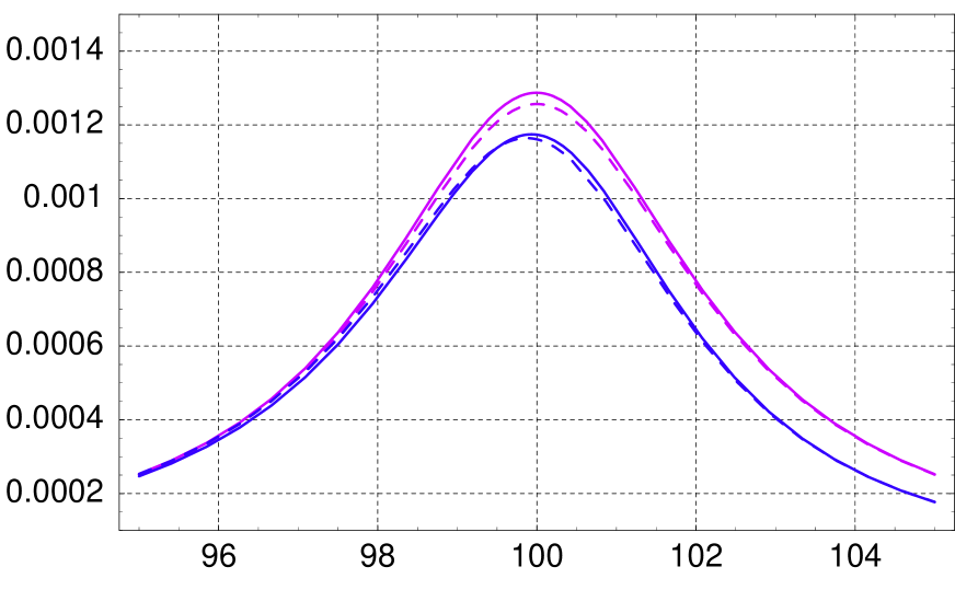
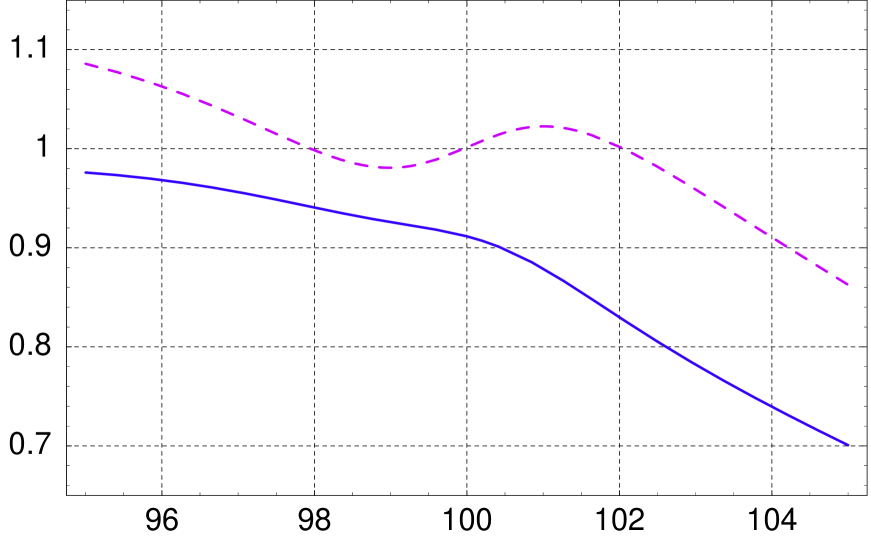
We computed the total cross section from the forward scattering amplitude. Fig. 1 (left side) shows the LO and NLO line-shape in the $\overline{\rm MS}$ scheme and pole scheme. The NLO correction amounts to 10% at the peak and to up to 30% in the resonant region. The right panel shows the ratio of the LO over the NLO line-shape. In the absence of data we performed a fit of the NLO line-shape to a Breit-Wigner and we plot the ratio of the NLO result to the Breit-Wigner fit. As can be nicely seen from Fig. 1 (right side) the deviation between NLO and the Breit-Wigner amounts to up to 15%. Furthermore, the value of the mass fitted from the Breit-Wigner differs from the input mass (the true value) by $160\,\mbox{MeV}$. This shows explicitly that for precision studies a proper theoretical prediction should be used, rather than a Breit-Wigner fit, which produce sizable shifts in the mass prediction.

Figure 1: Left: line shape (in $\mbox{GeV}^{-2}$) in the $\overline{\rm MS}$ scheme (solid) and pole scheme (dashed) at LO (upper magenta/light grey curves) and NLO (lower blue/dark grey curves) as a function of the center-of-mass energy in GeV. Right: The ratio of the NLO to the LO line shape in the $\overline{\rm MS}$ scheme (solid blue/dark grey curve) and the ratio of the NLO $\overline{\rm MS}$ line shape to a Breit-Wigner fit of the NLO result (dashed magenta/light grey curve).

4 Concluding remarks

The perturbative treatment of unstable particles requires a partial summation of the perturbative series, however we believe that the guiding principle was not understood. The breakdown of PT is related to the appearance of a second small parameter $\delta$, besides the coupling $\alpha$. We take the attitude that this is the characteristic feature of the problem, so that in a theory that formulates this double-expansion correctly, other issues like resummation, gauge invariance and unitarity should follow automatically. Since it is a two-scale problem ($\Gamma\ll M$) an effective theory is the natural framework to formulate such an expansion. The advantages of using effective theory methods are

• calculations are split into well-defined pieces (matching, matrix elements, loop calculations in the effective theory …), so that the calculation is efficient and transparent;

• a power counting scheme in the small parameters ($\alpha$, $\delta$) allows one to identify terms required to achieve a certain accuracy prior to performing the actual calculation;

• the effective theory provides a set of simpler Feynman rules which allows one to compute the minimal set of terms required at the given accuracy. Since one never computes “too much”, calculations are as simple as possible;

• calculations can be extended in principle to any order in $\alpha,\delta$, at the price of performing complicated, but standard loop integrals;

• since the expansion has been organized in such a way so as to account for kinematical enhancements the PT series in the effective theory converges rapidly;

• gauge invariance is automatic.

Despite the simplicity of the model considered (abelian theory, scalar particle), all necessary ingredients are provided for the formalism to be applied to any general case. Natural extensions concern non-inclusive kinematics, which requires a formalism to expand the real phase-space and generally implies that more collinear directions are relevant, and to pair-production of unstable particles, in which case the effective Lagrangian will contain two terms similar to eq. (5) describing the propagation of the two particles with different velocity vectors.

References

- [1] F. J. Dyson, Phys. Rev. 75 (1949) 486.
- [2] G. Lopez Castro, J. L. Lucio and J. Pestieau, Mod. Phys. Lett. A 6, 3679 (1991).
-
[3]
U. Baur and D. Zeppenfeld,
Phys. Rev. Lett. 75, 1002 (1995),
E. N. Argyres et al., Phys. Lett. B 358 (1995) 339;
W. Beenakker et al., Nucl. Phys. B 500 (1997) 255;
G. Passarino, Nucl. Phys. B 574 (2000) 451. -
[4]
R. G. Stuart,
Phys. Lett. B 262 (1991) 113;
A. Aeppli, G. J. van Oldenborgh and D. Wyler, Nucl. Phys. B 428 (1994) 126. -
[5]
W. Beenakker, F. A. Berends and A. P. Chapovsky,
Nucl. Phys. B 548 (1999) 3;
A. Denner, S. Dittmaier, M. Roth and D. Wackeroth, Nucl. Phys. B 587 (2000) 67;
Phys. Lett. B 475 (2000) 127;
S. Jadach et al., Phys. Rev. D 61 (2000) 113010. - [6] A. Denner, S. Dittmaier, M. Roth and D. Wackeroth, Nucl. Phys. B 560, 33 (1999).
- [7] V. A. Khoze, W. J. Stirling and L. H. Orr, Nucl. Phys. B 378, 413 (1992).
- [8] A. P. Chapovsky, V. A. Khoze, A. Signer and W. J. Stirling, Nucl. Phys. B 621, 257 (2002).
- [9] M. Beneke and V. A. Smirnov, Nucl. Phys. B 522, 321 (1998).
- [10] M. Beneke, A. P. Chapovsky, A. Signer and G. Zanderighi, hep-ph/0401002 and Nucl. Phys. B 686, 205 (2004).
[11]
E. Eichten and B. Hill,
Phys. Lett. B 234 (1990) 511;
H. Georgi, Phys. Lett. B 240 (1990) 447;
B. Grinstein, Nucl. Phys. B 339 (1990) 253. -
[12]
C. W. Bauer, S. Fleming and M. E. Luke,
Phys. Rev. D 63 (2001) 014006;
C. W. Bauer, S. Fleming, D. Pirjol, and I. W. Stewart, Phys. Rev. D 63 (2001) 114020;
C. W. Bauer, D. Pirjol, and I. W. Stewart, Phys. Rev. D 65 (2002) 054022;
M. Beneke, A. P. Chapovsky, M. Diehl and Th. Feldmann, Nucl. Phys. B 643 (2002) 431;
M. Beneke and Th. Feldmann, Phys. Lett. B 553 (2003) 267.