hep-ph/0405110

CERN–TH/2004-069, UMN–TH–2307/04, FTPI–MINN–04/18

Very Constrained Minimal Supersymmetric Standard Models

John Ellis¹, Keith A. Olive², Yudi Santoso² and Vassilis C. Spanos^{2 1}TH Division, CERN, Geneva, Switzerland
²William I. Fine Theoretical Physics Institute,
University of Minnesota, Minneapolis, MN 55455, USA

Abstract

We consider very constrained versions of the minimal supersymmetric extension of the Standard Model (VCMSSMs) which, in addition to constraining the scalar masses $m_{0}$ and gaugino masses $m_{1/2}$ to be universal at some input scale, impose relations between the trilinear and bilinear soft supersymmetry breaking parameters $A_{0}$ and $B_{0}$. These relations may be linear, as in simple minimal supergravity models, or nonlinear, as in the Giudice-Masiero mechanism for generating the Higgs-mixing $\mu$ term. We discuss the application of the electroweak vacuum conditions in VCMSSMs, which may be used to make a prediction for $\tan\beta$ as a function of $m_{0}$ and $m_{1/2}$ that is usually unique. We baseline the discussion of the parameter spaces allowed in VCMSSMs by updating the parameter space allowed in the CMSSM for fixed values of $\tan\beta$ with no relation between $A_{0}$ and $B_{0}$ assumed a priori, displaying contours of $B_{0}$ for a fixed input value of $A_{0}$, incorporating the latest CDF/D0 measurement of $m_{t}$ and the latest BNL measurement of $g_{\mu}-2$. We emphasize that phenomenological studies of the CMSSM are frequently not applicable to specific VCMSSMs, notably those based on minimal supergravity, which require $m_{0}=m_{3/2}$ as well as $A_{0}=B_{0}+m_{0}$. We then display $(m_{1/2},m_{0})$ planes for selected VCMSSMs, treating in a unified way the parameter regions where either a neutralino or the gravitino is the LSP. In particular, we examine in detail the allowed parameter space for the Giudice-Masiero model.

CERN–TH/2004-069

May 2004

1 Introduction

Supersymmetry is one of the most appealing extensions of the Standard Model (SM), for many reasons including the hierarchy problem, its necessity in string theory, unification of the SM gauge couplings, the suggestion of a light Higgs boson, the possibility that the astrophysical cold dark matter might be provided by the lightest supersymmetric particle (LSP) and (just possibly) the anomalous magnetic moment of the muon, $g_{\mu}-2$. However, supersymmetry is a general framework that accommodates many new degrees of freedom. The simplest possible realization of supersymmetry is the minimal supersymmetric extension of the SM (MSSM). Four types of supersymmetry-breaking parameters appear in the MSSM: scalar masses $m_{0}$, gaugino masses $m_{1/2}$, trilinear couplings $A$ and a bilinear coupling $B$ in the Higgs sector. In the MSSM alone, the number of free parameters associated with soft supersymmetry breaking exceeds 100, unless one assumes some degree of universality for the sparticles with different quantum numbers and flavours. In phenomenological studies of supersymmetry, the values of $m_{0}$ for the different sflavours are often constrained to be universal at some input GUT scale, as are the values of $m_{1/2}$ for the different SM gauge group factors, and the $A$ parameters corresponding to different SM Yukawa couplings, a framework often called the CMSSM.

One may go even further, and assume some relation(s) between the parameters $m_{0},m_{1/2}$, $A$, $B$ and the gravitino mass $m_{3/2}$. In particular, many very constrained versions of the MSSM (VCMSSMs) derive or postulate relations between the $A$ and $B$ parameters, which we parametrize as $A\equiv{\hat{A}}m_{0},B\equiv{\hat{B}}m_{0}$. These relations may be linear: for example, generic minimal supergravity models predict that ${\hat{B}}={\hat{A}}-1$ [1, 2] as well as $m_{0}=m_{3/2}$, and the simplest Polonyi model [3] of supersymmetry breaking further predicts that $|{\hat{A}}|=3-\sqrt{3}$ [4]. On the other hand, a prominent example of a nonlinear relation is

$$\hat{B}=\frac{2\hat{A}-3}{\hat{A}-3},$$ (1)

which appears in the Giudice-Masiero mechanism [5] for generating the $\mu$ term.

In the CMSSM, one may regard $m_{0},m_{1/2}$ and $A$ as independent parameters, and use the two electroweak vacuum conditions resulting from the specification of $m_{Z}$ and the ratio of Higgs vacuum expectation values, $\tan\beta$, to fix $|\mu|$ and the pseudoscalar Higgs mass $m_{A}$, which is equivalent to fixing ${\hat{B}}$. As we show in this paper with some explicit examples, the value of ${\hat{B}}$ that results for any given choice of $m_{0},m_{1/2}$ and ${\hat{A}}$ may not correspond to any plausible theoretical model. Conversely, in a VCMSSM where ${\hat{B}}$ is fixed in terms of ${\hat{A}}$, one can use the electroweak vacuum conditions to predict $\tan\beta$ as a function of $m_{0},m_{1/2}$ and ${\hat{A}}$. In a previous paper [6], we demonstrated this type of prediction for a few specific VCMSSMs with linear relations between ${\hat{A}}$ and ${\hat{B}}$, including minimal supergravity, with the simplest Polonyi model as a special case.

In this paper, we extend the previous discussion to include the Giudice-Masiero model. In this case, in addition to the relation (1) between $\hat{B}$ and $\hat{A}$, the value of $\mu$ is in principle also predicted as

$$\left|\frac{\mu}{m_{0}}\right|=\left|\lambda\frac{\hat{A}-3}{\sqrt{3}}\right|$$ (2)

where $\lambda/M_{Pl}$ is the coupling between a hidden sector superfield and the two Higgs superfields. The value of $\lambda$ is presumably not completely arbitrary: for example, one should probably require $|\lambda|\mathrel{\hbox to0.0pt{\raise 2.15277pt\hbox{$<$}\hss}{\lower 2.15277pt\hbox{$\sim$}}}O(1)$. This bound on $|\lambda|$ in turn imposes a range on the ratio $\mu/m_{0}$ for a given $\hat{A}$. Since the value of $|\mu|$ is an output quantity in our approach to VCMSSMs, one must check that $|\lambda|$ is not very large, which could in principle restrict the ranges of the input parameters.

The first step in this paper is to discuss the application of the electroweak vacuum conditions. In principle, more than one value of $\tan\beta$ might be consistent with a given VCMSSM for some specific choice of $(m_{0},m_{1/2})$ [7]. In practice, over large regions of the $(m_{0},m_{1/2})$ we find only one solution for $\tan\beta$, as we explain in some detail. We also discuss the renormalization of the input relation between $A$ and $B$ in a generic VCMSSM, including the relation between the input and electroweak-scale values of $B$ and the one-loop threshold corrections at the electroweak scale.

The second step is to update previous analyses of the CMSSM, including some updates in calculations of the supersymmetric particle spectrum, as well as the latest information on $m_{t}$, $g_{\mu}-2$, $b\to s\gamma$ and $B_{s}\to\mu^{+}\mu^{-}$. We demonstrate that the values of ${\hat{B}}$ required in the CMSSM for generic values of $\tan\beta$ and ${\hat{A}}$ do not fit within favoured VCMSSM frameworks, such as those based on minimal supergravity or the Giudice-Masiero model.

We then discuss the $(m_{0},m_{1/2})$ planes for some specific VCMSSMs, taking into account the fact that minimal supergravity models predict that $m_{0}=m_{3/2}$ before renormalization, which is not necessarily the case in a generic CMSSM. This relation enables one to delineate the regions where the LSP is the lightest neutralino $\chi$, the lighter ${\tilde{\tau}}$ or the gravitino ${\tilde{G}}$. We present unified descriptions of the $\chi$ and ${\tilde{G}}$ LSP regions for some specific VCMSSMs, incorporating the constraints on decays of the next-to-lightest supersymmetric particle (NSP) into a gravitino LSP that are imposed by concordance between the Big-Bang nucleosynthesis (BBN) and cosmological microwave background (CMB) determinations of the baryon-to-entropy ratio [8, 9, 10, 11]. Finally, we discuss the Giudice-Masiero model in more detail, finding that the implied values of $|\lambda|$ in allowed regions of parameter space are generally $\mathrel{\hbox to0.0pt{\raise 2.15277pt\hbox{$>$}\hss}{\lower 2.15277pt\hbox{$\sim$}}}O(1)$, particularly in the gravitino LSP region.

2 Summary of Models of Supersymmetry Breaking

As discussed in [6], we assume an $N=1$ supergravity framework, interpreted as a low-energy effective field theory. In minimal supergravity models, the Kähler function $K$ that describes the kinetic terms for the chiral supermultiplets $\Phi\equiv(\zeta,\phi)$, where the $\zeta$ represent hidden-sector fields and the $\phi^{i}$ observable-sector fields, has the form $K=\Sigma_{i}|\Phi^{i}|^{2}$. We denote derivatives of $K$ with respect to the chiral superfields by $K_{i}\equiv\partial K/\partial\phi^{i}$, etc. In the minimal supergravity case, we have $K^{i}={\phi^{i}}^{*}+{W^{i}}/W$, $K_{i}=\phi_{i}+W_{i}^{*}/W^{*}$, and $({K^{-1}})^{j}_{i}=\delta^{j}_{i}$, and the resulting scalar potential is (in units where the Planck mass is unity)

$$V(\phi,\phi^{*})\;=\;e^{\phi_{i}{\phi^{i}}^{*}}\left[|W^{i}+{\phi^{i}}^{*}W|^{2}-3|W|^{2}\right].$$ (3)

It is then apparent that the soft supersymmetry-breaking scalar masses $m_{0}$ are universal at the input GUT scale, with [1]

$$m_{0}^{2}\;=\;m_{3/2}^{2},$$ (4)

where $m_{3/2}$ is the gravitino mass and we assume that the tree-level cosmological constant vanishes. If we further assume that the superpotential $W(\Phi)$ may be separated into pieces $f$ and $g$ that are functions only of observable-sector fields $\phi^{i}$ and hidden-sector fields $\zeta$, respectively, then the soft supersymmetry-breaking trilinear terms $A_{0}$ and bilinear terms $B_{0}$ are also universal, and are related by [1]

$$B_{0}\;=\;A_{0}-m_{3/2},$$ (5)

so that

$${\hat{B}}\;=\;{\hat{A}}-1,$$ (6)

which is one of the principal options we studied in [6] and discuss further below.

The simplest model for local supersymmetry breaking in minimal supergravity [3] has just one additional chiral multiplet $\zeta$ in addition to the observable matter fields $\phi_{i}$, with a superpotential that is separable in this so-called Polonyi field and the observable fields $\phi_{i}$: $W=f(\phi)+g(\zeta)$. It takes the simple form

$$g(\zeta)\;=\;\nu(\zeta+\beta),$$ (7)

where we impose $|\beta|=2-\sqrt{3}$ to ensure that the cosmological constant vanishes. Assuming $\beta$ to be positive, and using $\langle\zeta\rangle=\sqrt{3}-1$, we have [4] the universal soft trilinear supersymmetry-breaking terms

$$\hat{A}\;=\;(3-\sqrt{3})m_{3/2},$$ (8)

and universal bilinear soft supersymmetry-breaking terms

$$\hat{B}\;=\;(2-\sqrt{3})m_{3/2},$$ (9)

whose consequences we explored in [6] and discuss further below.

In the simplest version of the Giudice-Masiero (GM) mechanism [5], in addition to minimal supergravity kinetic terms in the observable and hidden sectors, and a separable superpotential $W=f+g$, one postulates a coupling

$$K(\phi,\zeta)\;\ni\;\lambda\zeta^{\dagger}H_{1}H_{2},$$ (10)

where $H_{1,2}$ are the two Higgs supermultiplets in the MSSM. Assuming that the cosmological constant vanishes, the term (10) generates a Higgs mixing term (2). This mechanism also yields the nonlinear relation between $\hat{B}$ and $\hat{A}$ given in (1), whose consequences we explore below.

As already remarked, minimal supergravity models predict a relation (4) between $m_{0}$ and the gravitino mass, which is not necessarily true in the generic CMSSM. This relation enables us to delineate the regions of VCMSSM parameter space where the LSP is a neutralino, the lighter ${\tilde{\tau}}$ or the gravitino. The astrophysical and cosmological constraints on gravitino dark matter have been recently re-examined [8, 9], taking also into account the constraints on decays of the next-to-lightest supersymmetric particle (NSP) arising from comparing the BBN and CMB constraints on the baryon-to-entropy ratio [10, 11]. In our later discussions of VCMSSMs, we give unified treatments of the parts of $(m_{1/2},m_{0})$ planes where the LSP is a neutralino, the lighter ${\tilde{\tau}}$ and the gravitino.

3 The Electroweak Vacuum in VCMSSMs

In the general CMSSM, we start with the following set of input parameters defined at the GUT scale: $m_{1/2}$, $m_{0}$, $A_{0}$, $B_{0}$ and the Higgs mixing parameter $\mu_{0}$. At tree level, the electroweak vacuum is specified by the following two conditions:

$$m_{Z}^{2} = {2(m_{1}^{2}+\mu^{2}-(m_{2}^{2}+\mu^{2})\tan^{2}\beta)\over(\tan^{2}\beta-1)},$$ (11)

$$\sin 2\beta = {-2B\mu}/(m_{1}^{2}+m_{2}^{2}+2\mu^{2}),$$ (12)

and the pseudoscalar neutral Higgs mass $m_{A}$ is determined by

$$m_{A}^{2}\;=\;m_{1}^{2}+m_{2}^{2}+2\mu^{2},$$ (13)

where $m_{1}$ and $m_{2}$ are the soft supersymmetry-breaking masses for the two Higgs doublets at the electroweak scale. These as well as $\mu$ and $B$ are assumed to be evaluated by renormalization-group equation (RGE) running from the input values. One may, alternatively, solve for $\mu$ and $B$ in terms of $m_{Z}$ and $\tan\beta$:

$$\mu^{2} = \frac{m_{1}^{2}-m_{2}^{2}\tan^{2}\beta+\frac{1}{2}m_{\scriptscriptstyle Z}^{2}(1-\tan^{2}\beta)+\Delta_{\mu}^{(1)}}{\tan^{2}\beta-1+\Delta_{\mu}^{(2)}}$$

$$B\mu = -{1\over 2}(m_{1}^{2}+m_{2}^{2}+2\mu^{2})\sin 2\beta+\Delta_{B}$$ (14)

where we have now included the loop corrections $\Delta_{B}$ and $\Delta_{\mu}^{(1,2)}$ required to relate the RGE values to the corresponding quantities evaluated at $m_{Z}$ [12, 13, 14], and here $m_{1,2}\equiv m_{1,2}(m_{Z})$ . In most treatments of the CMSSM, $m_{1/2}$, $m_{0}$, $A_{0}$ and $\tan\beta$ are taken as inputs, and the conditions (14) are used to determine $\mu$, $B$ and the CP-odd Higgs mass $m_{A}$.

As discussed in [6], in a VCMSSM where $B$ is determined in advance in terms of $A$, it is convenient to use the electroweak vacuum conditions (14) to determine $\tan\beta$ as a function of $m_{0}$ and $m_{1/2}$ for some input value of $A$. However, since $\Delta_{\mu}$ depends on $\tan\beta$, and $\Delta_{B}$ depends on both $\mu$ and $\tan\beta$ in a nonlinear way, it is not possible to write down an analytical solution for $\tan\beta$. Moreover, it was shown in [7] using an RGE-improved tree-level calculation for $\tan\beta$ in the minimal supergravity model that there may be up to three possible solutions for $\tan\beta$ for any given choices of $m_{1/2},m_{0}$, and $A_{0}$. We remarked previously [6] that we typically find just one solution with a moderately low value of $\tan\beta$, that multiple solutions exist only for $m_{t}<153$ GeV, and that $B$ always increases monotonically with $\tan\beta$ over the range $5<\tan\beta<55$ in our calculations. Thus, a given value of $m_{1/2}$, $m_{0}$, $A_{0}$ and $sgn(\mu)$ always corresponds, in our analysis, to a definite value for $\tan\beta$. Since this is important for our treatment of VCMSSMs, we now illustrate this point in more detail.

We show in Fig. 1 some examples of the necessary input values of $B_{0}$ as functions of $\tan\beta$, for four representative choices of $(m_{0},m_{1/2})$ and $\mu>0$. We use $m_{t}=178$ GeV as suggested by the latest CDF and D0 results [15]. We see that $B_{0}$ generally increases monotonically for all positive values of $A_{0}$, and also for some negative values of $A_{0}$. This is also true for $\mu<0$, as seen in Fig. 2. These observations immediately imply that, in any VCMSSM that predicts a unique value of $B_{0}$ for a given value of $A_{0}$, there will be (at most) a unique value of $\tan\beta$ where the VCMSSM relation is obeyed.

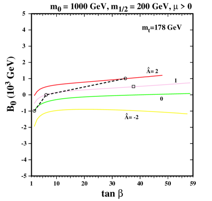
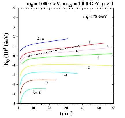
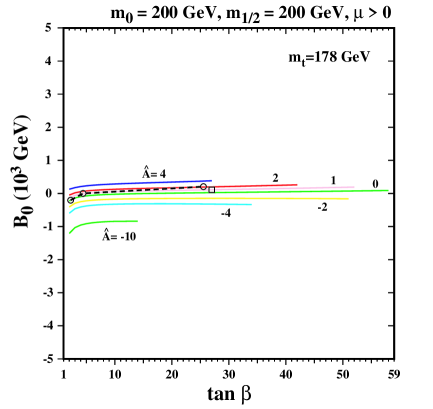
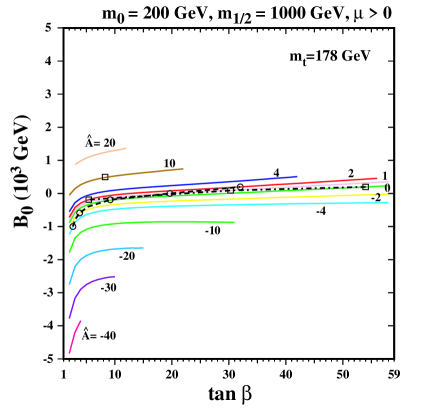
Figure 1: Values of $B_{0}$ as functions of $\tan\beta$ for $\mu>0$ and $(m_{1/2},m_{0})=$ (a) $(200,1000)$ GeV, (b) $(1000,1000)$ GeV, (c) $(200,200)$ GeV and (d) $(1000,200)$ GeV. Solutions for ${\hat{B}}={\hat{A}}-1$ case are denoted by small circles, which are connected by dashed lines. Solutions in the case of the Giudice-Masiero mechanism are denoted by small squares, connected by dot-dashed lines when possible.

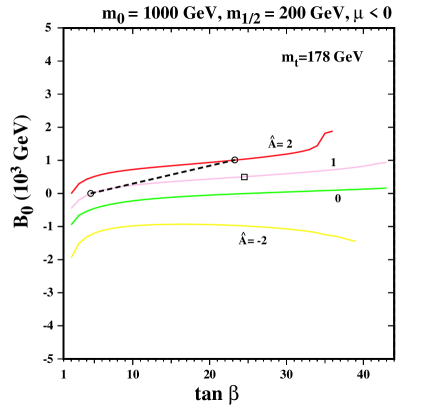
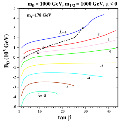
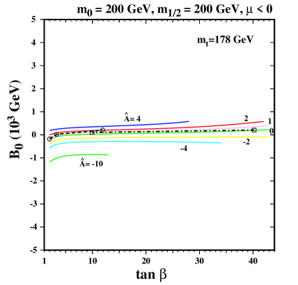
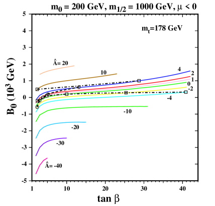
Figure 2: As in Fig. 1, but for $\mu<0$.

We note, however, that there are some particular negative values of $A_{0}$ for which the required value of $B_{0}$, after rising when $\tan\beta$ is small, decreases slightly at large $\tan\beta$. This raises the possibility that there might be two allowed values of $\tan\beta$ in some restricted set of VCMSSMs. One example is when $m_{1/2}=200$ GeV, $m_{0}=1000$ GeV, $\mu>0$, ${\hat{A}}\simeq-2$ and ${\hat{B}}\simeq-1.5$, as seen in panel (a) of Fig. 1, and there are some other examples in other panels of Figs. 1 and 2. However, in practice, such multiple solutions do not exist in the specific VCMSSMs that we study in this paper.

To illustrate this more explicitly, we indicate by small circles in Figs. 1 and 2 the values of $\tan\beta$ where the minimal supergravity condition ${\hat{B}}={\hat{A}}-1$ is satisfied, for a few specific values of ${\hat{A}}$, and we join these points by dashed lines. For each value of ${\hat{A}}$ there is clearly only one consistent choice of $\tan\beta$ for any given choice of $(m_{1/2},m_{0})$. We also show solutions for the Giudice-Masiero mechanism case, indicated by small squares.

Note that we do not obtain solutions for $\hat{B}$ for all choices of $\hat{A}$. For example, in Fig. 1a, we show solutions only for $\hat{A}=0,1$ and 2 for $\hat{B}=\hat{A}-1$ and $\hat{A}=1$ for the Giudice-Masiero model. In the minimal supergravity case, when $\hat{A}$ is reduced, $\hat{B}$ is also reduced driving the solution to smaller values of $\tan\beta$. Very quickly these solutions drop below $\tan\beta=2$ and, below $\tan\beta\sim 1.7$, the RGEs do not provide solutions to the sparticle spectra due to a divergence in the top quark Yukawa coupling at the unification scale. Similarly when $\hat{A}$ is large, the solution is driven to very large values of $\tan\beta$ where again no solutions to the RGEs are found. In the case of the GM model, the slope of $B_{0}$ vs $\tan\beta$ is very small, and small changes in $\hat{A}$ lead to large changes in $\tan\beta$. Note also that in the GM model, there are often two branches of solutions which are disconnected. This is seen for example in Figs. 1d and 2d. This is due to the relation (1) which separates solutions at $\hat{A}=3$.

In order to have an analytical feel for the solutions for $B_{0}$ shown in Fig. 1 and 2, we show in Fig. 3 the values of $B_{0}$ at the input GUT scale, the tree-level values at the electroweak scale and the full values of $B(M_{W})$ as functions of $\tan\beta$, (a) for $\mu>0$ and (b) for $\mu<0$, in both cases for $(m_{1/2},m_{0})=(200,200)$ GeV. The tree-level value of $B$ at the electroweak scale is defined as

$$B_{tree}\;\equiv\;\frac{(m_{1}^{2}+m_{2}^{2}+2\mu^{2})\sin 2\beta}{-2\mu},$$ (15)

and as one can see $B_{tree}$ tends to 0 as $\tan\beta$ is increased. The ‘full’ values are calculated including one-loop electroweak threshold corrections, and $B_{0}$ is then the result of running the RGEs from the weak scale to the unification scale. In the $\mu>0$ case, we see in Fig. 3 that $B_{0}$ is systematically larger than the tree-level value of $B(M_{W})$, which is in turn larger than its full value. However, even in this case $B(M_{W})$ increases monotonically with $\tan\beta$. The situation is rather different for $\mu<0$, where we see that the sign of the loop correction depends on the value of $\tan\beta$, vanishing for $\tan\beta\simeq 21$. As a result, the full value of $B(M_{W})$ and hence $B_{0}$ increase monotonically with $\tan\beta$. Had we neglected the 1-loop corrections to $B$ and ran the RGEs up to the unification scale, we could obtain a non-monotonic solution for $B_{0}$ with respect to $\tan\beta$ (for example, a solution with a minimum value of $B_{0}$) leading to multiple solutions of $\tan\beta$ for a fixed value of $\hat{A}$ [18]. Thus, Fig. 3 indicates the importance of the loop correction in determining the number of solutions.

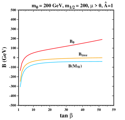
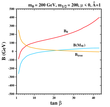
Figure 3: The values of $B_{0}$, the electroweak tree-level and full $B(M_{W})$, as functions of $\tan\beta$ for (a) $\mu>0$ and (b) $\mu<0$, both for $(m_{1/2},m_{0})=(200,200)$ GeV and ${\hat{A}}=1$.

4 Updated Constraints on the CMSSM

The standard LEP constraints and cosmological constraints on the CMSSM have been discussed previously in many places [19, 20], so we do not discuss them further here, except to recall that we use the WMAP range $0.094<\Omega_{\chi}h^{2}<0.129$ [21] for the relic density of the LSP, assumed to be the lightest neutralino $\chi$. However, there are three new experimental developments that we should like to mention. One is the new value $m_{t}=178.0\pm 4.3$ GeV recently reported by the CDF and D0 collaborations [15], another is the evolution in the possible discrepancy between the experimental measurement of $g_{\mu}-2$ and the value calculated in the SM, and the other is a recent improved upper limit on the branching ratio for $B_{s}\to\mu^{+}\mu^{-}$.

The new value of $m_{t}$ affects the CMSSM parameter space in three important ways. One is to alter the calculation of the lightest MSSM Higgs boson mass $m_{h}$, and hence the lower limit on $m_{1/2}$ inferred from the LEP lower limit $m_{h}>114.4$ GeV. For example, in panel (a) of Fig. 4 for $\tan\beta=10$ and $\mu>0$, the lower limit on $m_{1/2}$ is reduced by about 50 GeV when one increases $m_{t}$ from 175 GeV to the value of 178 GeV shown here. A second effect is to alter the calculation of the rapid-annihilation funnels shown in panels (c) and (d) of Fig. 4 for $\tan\beta=35$ and $\mu<0$ and for $\tan\beta=50$ and $\mu>0$, respectively. The sensitivity of these regions to $m_{t}$ and large $\tan\beta$ was discussed earlier [22] in the context of the observability of the Higgs boson at hadron colliders. Finally, the larger value of $m_{t}$ increases significantly the value of $m_{0}$ where the focus-point region may be found [23]. For example, for $\tan\beta=10$ and $\mu>0$, we now find a focus-point region only for $m_{0}\mathrel{\hbox to0.0pt{\raise 2.15277pt\hbox{$>$}\hss}{\lower 2.15277pt\hbox{$\sim$}}}7$ TeV for $m_{1/2}\mathrel{\hbox to0.0pt{\raise 2.15277pt\hbox{$>$}\hss}{\lower 2.15277pt\hbox{$\sim$}}}250$ GeV. We do not discuss focus points further in this paper.

The BNL $g_{\mu}-2$ experiment recently announced a new determination using $\mu^{-}$ and a final combined value using all their $\mu^{\pm}$ data [24]. Comparing with the SM calculations of Davier et al. [25], they quote a discrepancy of $a_{\mu}\equiv(g_{\mu}-2)/2$ with the SM amounting to

$$\delta a_{\mu} = (27\pm 10)\times 10^{-10}\;(e^{+}e^{-}{\rm~{}data})$$ (16)

$$= (12\pm 9)\times 10^{-10}\;(\tau{\rm~{}data}).$$

Another calculation of the SM contribution to $(g_{\mu}-2)$ using just the $e^{+}e^{-}$ data [26] yielded a slightly larger discrepancy:

$$\delta a_{\mu} = (32\pm 10)\times 10^{-10}\;(e^{+}e^{-}{\rm~{}data})$$ (17)

There has subsequently been a new SM calculation of the hadronic vacuum polarization contribution by de Trocóniz and Ynduráin [27], who quote

$$\delta a_{\mu} = (27\pm 8)\times 10^{-10}\;(e^{+}e^{-}{\rm~{}data})$$ (18)

$$= (19\pm 8)\times 10^{-10}\;(\tau{\rm~{}and~{}}e^{+}e^{-}{\rm~{}data}).$$

However, neither of these evaluations include the recent re-evaluation of the light-by-light contribution to $a_{\mu}$ by Melnikov and Vainshtein [28], which decreases the discrepancy with the SM by about $4\times 10^{-10}$ compared with (18). Therefore, for the purposes of the subsequent discussion, we show contours corresponding to

$$\delta a_{\mu}\;=\;(15\pm 8)\times 10^{-10}.$$ (19)

We exhibit this constraint at the 2-$\sigma$ level, in which case its effect is essentially to exclude the option $\mu<0$ but allow most of the $(m_{1/2},m_{0})$ plane for $\mu>0$, apart from a region of small $m_{1/2}$ and $m_{0}$. However, we are well aware that the range (19) is open to question, particularly in view of the discrepancy between the estimates of the SM contribution based on $e^{+}e^{-}$ and $\tau$ data, and, to a lesser extent, the uncertainty in the light-by-light contribution. Therefore, we use (19) only as an indication, and by no means a rigid constraint on the parameter space of the CMSSM or any VCMSSM. In particular, we do not discard the option $\mu<0$.

Finally, we note that the CDF Collaboration have recently published an improved experimental upper limit on the branching ratio for $B_{s}\to\mu^{+}\mu^{-}$ [29], namely $5.8\times 10^{-7}$. Since the branching ratio for this decay $\propto\tan^{6}\beta$ in the CMSSM, this constraint is potentially important at large $\tan\beta$. We find that this constraint is currently still ‘covered’ by the constraints from $b\to s\gamma$, $m_{h}$ and $g_{\mu}-2$, but this situation may change in the near future.

In preparing the $(m_{1/2},m_{0})$ planes in Fig. 4 and the subsequent figures, we have updated our code by making improvements that have impacts principally in the rapid-annihilation funnels and focus-point regions . Their effects are smaller than the other effects mentioned above.

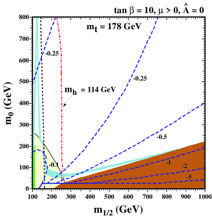
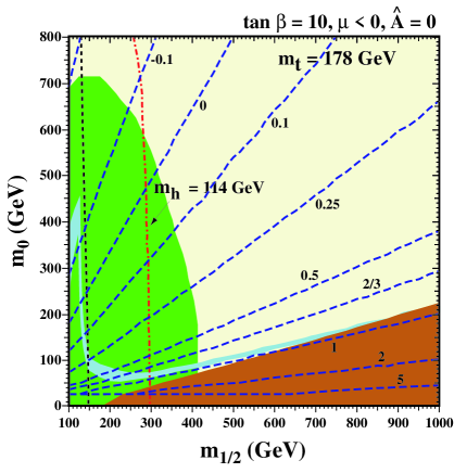
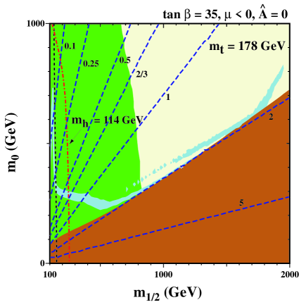
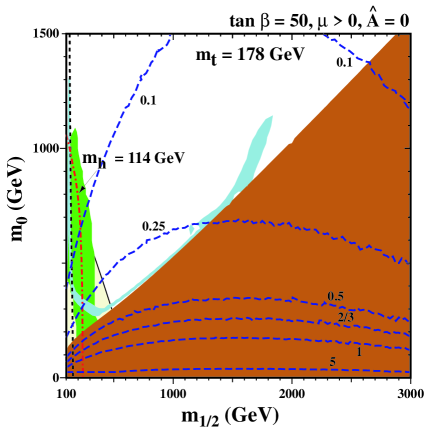
Figure 4: The $(m_{1/2},m_{0})$ planes in the CMSSM for (a) $\tan\beta=10,\mu>0$, (b) $\tan\beta=10,\mu<0$, (c) $\tan\beta=35,\mu<0$, and (d) $\tan\beta=50,\mu>0$, all for $\hat{A}=0$. In each panel, the region allowed by the WMAP cosmological constraint $0.094\leq\Omega_{\chi}h^{2}\leq 0.129$ has pale (turquoise) shading. The disallowed region where $m_{\tilde{\tau}_{1}}<m_{\chi}$ has dark (red) shading. The regions excluded by $b\rightarrow s\gamma$ have medium (green) shading, and those in panels (a,d) that are disfavoured by $g_{\mu}-2$ at the 2-$\sigma$ level have very light (yellow) shading with a thin (black) border. The contours $m_{\chi^{\pm}}=104$ GeV ($m_{h}=114$ GeV) are shown as near-vertical black dashed (red dot-dashed) lines. In addition, we show several contours of $\hat{B}$ as (blue) dashed lines. There is no allowed point compatible with the minimal supergravity condition ${\hat{B}}={\hat{A}}-1$ or the Giudice-Masiero model in these plots.

We show in Fig. 4 the $(m_{1/2},m_{0})$ planes for a popular set of CMSSM cases, namely (a) $\tan\beta=10,\mu>0$, (b) $\tan\beta=10,\mu<0$, (c) $\tan\beta=35,\mu<0$, and (d) $\tan\beta=50,\mu>0$, all for $\hat{A}=0$ . In each panel, as well as the ‘standard’ experimental and cosmological constraints, we have indicated some representative contours of $\hat{B}$ by (blue) dashed lines. We see that ${\hat{B}}\mathrel{\hbox to0.0pt{\raise 2.15277pt\hbox{$>$}\hss}{\lower 2.15277pt\hbox{$\sim$}}}0$ in almost all the $(m_{1/2},m_{0})$ planes exhibited, which is clearly incompatible with the minimal supergravity condition ${\hat{B}}={\hat{A}}-1$. This exemplifies the point that parameter choices allowed in the ‘standard’ CMSSM are often not allowed in favoured VCMSSMs. Specifically, the CMSSM cases shown in Fig. 4 could not be realized in minimal supergravity: one needs to choose smaller values of $\tan\beta$. A similar conclusion applies to the Giudice-Masiero model, which would require ${\hat{B}}=1$ for the case ${\hat{A}}=0$ considered here, although GM solutions are possible for $\mu<0$ if one discards the $g_{\mu}-2$ constraint and chooses $\tan\beta$ somewhat above 10.

Fig. 5 shows the corresponding $(m_{1/2},m_{0})$ planes for the same choices of $\tan\beta$ and the sign of $\mu$, but for $\hat{A}=+0.75$. In this case, the laboratory and cosmological constraints are not greatly different, even in the rapid-annihilation funnel regions . Now, however, there are some points where the minimal supergravity condition ${\hat{B}}={\hat{A}}-1$ is satisfied, as shown by the intersection of the $\hat{B}=-0.25$ line with the WMAP coannihilation region in Fig. 5a. For this choice of ${\hat{A}}$, the Giudice-Masiero model is also satisfied at a limited number of points, exemplified by the intersection of the $\hat{B}=2/3$ line with the WMAP funnel region in Fig. 5d.

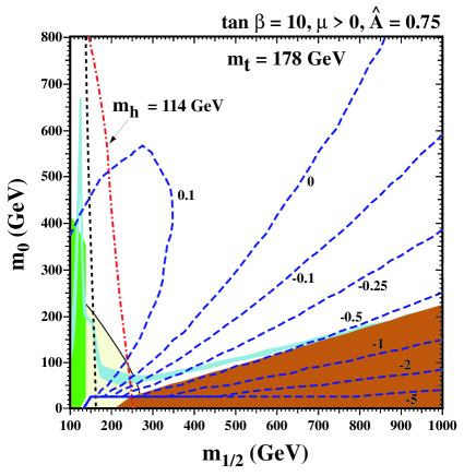
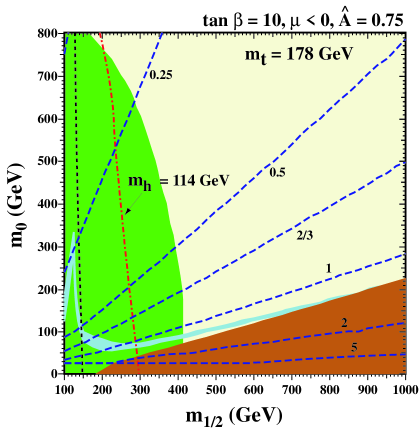
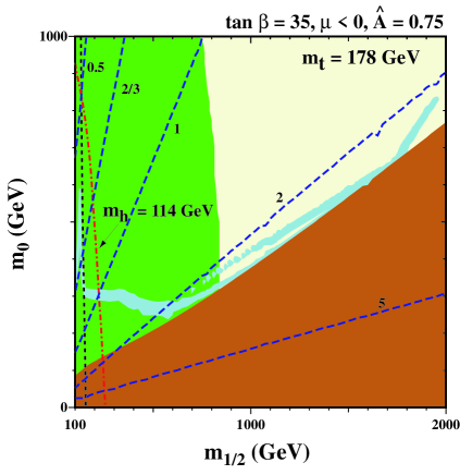
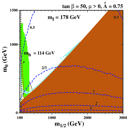
Figure 5: The $(m_{1/2},m_{0})$ planes in the CMSSM for the same values of $\tan\beta$ and the sign of $\mu$ as in Fig. 4, but here for $\hat{A}=+0.75$.

5 Examples of $(m_{1/2},m_{0})$ Planes in VCMSSMs

We now discuss the impacts of the above constraints on some specific VCMSSMs within the general framework of minimal supergravity, in which ${\hat{B}}={\hat{A}}-1$. As usual, we display these constraints in $(m_{1/2},m_{0})$ planes. For the reasons discussed earlier, we regard $\tan\beta$ as a dependent quantity that varies across these planes, rather than being a fixed quantity as in most CMSSM analyses. Another difference from most CMSSM analyses is that the latter generally consider only the possibility that the LSP is the lightest neutralino $\chi$, assuming implicitly that the gravitino mass $m_{3/2}$ is sufficiently large that the gravitino LSP possibility can be neglected. However, in minimal supergravity, one has $m_{3/2}=m_{0}$ (4) if the cosmological constant $\Lambda=0$, and the identity of the LSP varies over the $(m_{1/2},m_{0})$ plane. We have recently published an analysis which includes the possibility that the gravitino is the LSP possibility [8], taking into account the constraints imposed by Big-Bang nucleosynthesis (BBN) and the cosmic microwave background (CMB) data on decays of the next-to-lightest sparticle (NSP) into the gravitino, as well as the relic gravitino dark matter density itself. In this paper, we incorporate this analysis into a unified treatment of the neutralino and gravitino LSP regions of the $(m_{1/2},m_{0})$ planes in VCMSSMs.

We display in Fig. 6 the contours of $\tan\beta$ (solid blue lines) in the $(m_{1/2},m_{0})$ planes for selected values of ${\hat{A}}$, ${\hat{B}}$ and the sign of $\mu$. Also shown are the contours where $m_{\chi^{\pm}}>104$ GeV (near-vertical black dashed lines) and $m_{h}>114$ GeV (diagonal red dash-dotted lines). The regions excluded by $b\to s\gamma$ have medium (green) shading, and those where the relic density of neutralinos lies within the WMAP range $0.094\leq\Omega_{\chi}h^{2}\leq 0.129$ have light (turquoise) shading. The gravitino LSP and the neutralino LSP regions are separated by dark (chocolate) solid lines, and the WMAP relic-density strip for neutralinos is shown only above these lines. The regions disfavoured by $g_{\mu}-2$ at the 2-$\sigma$ level are very light (yellow) shaded.

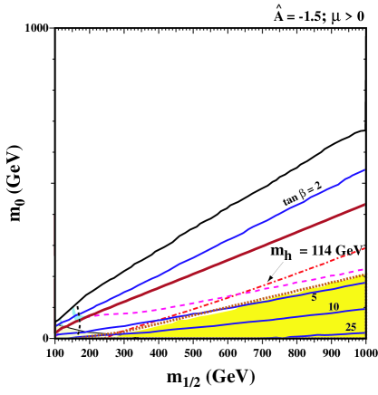
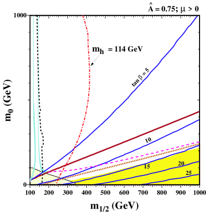
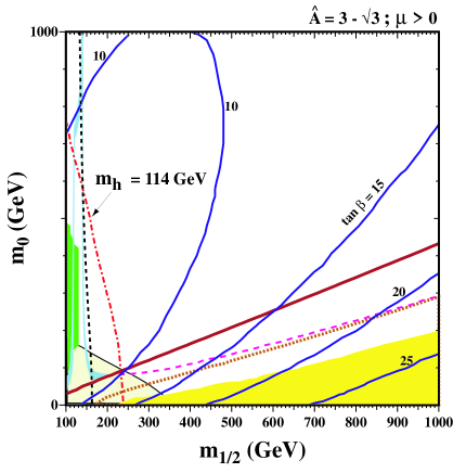
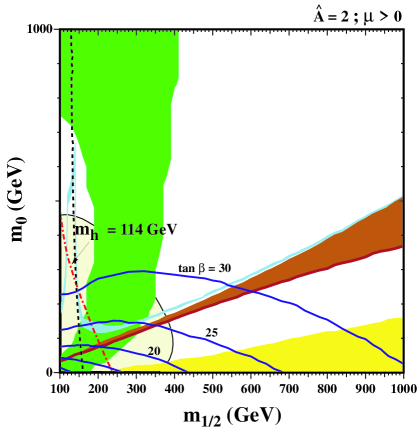
Figure 6: Examples of VCMSSM $(m_{1/2},m_{0})$ planes with contours of $\tan\beta$ superposed, for $\mu>0$ and (a) ${\hat{A}}=-1.5$, (b) ${\hat{A}}=0.75$, (c) the simplest Polonyi model with ${\hat{A}}=3-\sqrt{3}$, and (d) ${\hat{A}}=2.0$, all with ${\hat{B}}={\hat{A}}-1$. In each panel, we show the regions excluded by the LEP lower limits on MSSM particles and those ruled out by $b\to s\gamma$ decay [31] (medium green shading): the regions disfavoured by $g_{\mu}-2$ are very light (yellow) shaded, bordered by a thin (black) line. The dark (chocolate) solid lines in panels (a, b, c) separate the gravitino LSP regions (below). Panel (d) exhibits a dark (red) wedge where the LSP is the rapid ${\tilde{\tau}}_{1}$. The regions favoured by WMAP in the neutralino LSP case have light (turquoise) shading. The dashed (pink) line corresponds to the maximum relic density for the gravitino LSP, and regions allowed by BBN/CMB constraint on NSP decay are light (yellow) shaded.

If ${\hat{A}}$ has a large negative value, we do not find any consistent solutions to the electroweak vacuum conditions. This is reflected in panel (a) of Fig. 6, for $\mu>0$ and ${\hat{A}}=-1.5$, where there are no solutions above the topmost solid (black) line. The solid (blue) contours of $\tan\beta$ rise diagonally from low values of $(m_{1/2},m_{0})$ to higher values, with higher values of $\tan\beta$ having lower values of $m_{0}$ for a given value of $m_{1/2}$. The dash-dotted (red) $m_{h}=114$ GeV contour rises in a similar way, and regions above and to the left of this contour have $m_{h}<114$ GeV and are excluded. In particular, a neutralino LSP is excluded in this case. We exhibit in this and the other panels a gravitino LSP region, which was not studied in our previous exploration of VCMSSMs [6]. The relic density is acceptably low only below the dashed (pink) line. This excludes a supplementary domain of the $(m_{1/2},m_{0})$ plane, but the strongest constraint is provided by the BBN/CMB decay constraint (light, yellow shading), which requires $\tan\beta\mathrel{\hbox to0.0pt{\raise 2.15277pt\hbox{$>$}\hss}{\lower 2.15277pt\hbox{$\sim$}}}4.5$. In panels (b, c, d), the $m_{h}$ contour rises more vertically, but only in panel (d) is there any allowed neutralino LSP region. Panel (d) features an excluded dark (red) shaded wedge where the LSP is the ${\tilde{\tau}}_{1}$.

When ${\hat{A}}$ is increased to 0.75, as seen in panel (b) of Fig. 6, both the $\tan\beta$ and $m_{h}$ contours rise more rapidly with $m_{1/2}$. Again, there is no allowed neutralino LSP region. Within the gravitino LSP region, the $m_{h}$ and relic density constraints would both be compatible with $\tan\beta\mathrel{\hbox to0.0pt{\raise 2.15277pt\hbox{$>$}\hss}{\lower 2.15277pt\hbox{$\sim$}}}7.5$, but the BBN/CMB decay constraint imposes the stronger constraint that $\tan\beta\mathrel{\hbox to0.0pt{\raise 2.15277pt\hbox{$>$}\hss}{\lower 2.15277pt\hbox{$\sim$}}}13$. It is instructive to compare this figure with Fig. 5a, which both assume that $\hat{A}=0.75$. The most notable difference is that, here, fixing the gravitino mass to equal $m_{0}$ excludes the neutralino coannihilation region with $\hat{B}=-0.25$ and allows a region of the $(m_{1/2},m_{0})$ plane that would previously have been excluded because the LSP would have been the ${\tilde{\tau}}_{1}$.

An analogous pattern is seen in the simplest Polonyi model with ${\hat{A}}=3-\sqrt{3}$ shown in panel (c) of Fig. 6, where we note that the $\tan\beta$ contours have noticeable curvature. Once again, the neutralino LSP region is excluded, now by a combination of the Higgs and chargino mass bounds. At low $m_{0}$ in the gravitino LSP region, the $m_{h}$ and relic gravitino density constraints impose $\tan\beta\mathrel{\hbox to0.0pt{\raise 2.15277pt\hbox{$>$}\hss}{\lower 2.15277pt\hbox{$\sim$}}}10$ and the BBN/CMB decay constraint imposes $\tan\beta\mathrel{\hbox to0.0pt{\raise 2.15277pt\hbox{$>$}\hss}{\lower 2.15277pt\hbox{$\sim$}}}14$ .

We consider finally the case ${\hat{A}}=2.0$ shown in panel (d) of Fig. 6. In this case, there is a neutralino LSP region in the $\chi-{\tilde{\tau}}$ coannihilation strip. Without the $g_{\mu}-2$ constraint, the most severe constraint on this region is imposed by $b\to s\gamma$, requiring $\tan\beta\mathrel{\hbox to0.0pt{\raise 2.15277pt\hbox{$>$}\hss}{\lower 2.15277pt\hbox{$\sim$}}}25$, the $m_{h}$ constraint being much weaker. Imposing the $g_{\mu}-2$ constraint requires $\tan\beta\mathrel{\hbox to0.0pt{\raise 2.15277pt\hbox{$>$}\hss}{\lower 2.15277pt\hbox{$\sim$}}}27$. There is an excluded dark (red) shaded wedge where the LSP is the ${\tilde{\tau}}_{1}$. Below this appears a gravitino LSP region with acceptable relic density. Within this region, the $m_{h}$ and BBN/CMB decay constraints impose $\tan\beta\mathrel{\hbox to0.0pt{\raise 2.15277pt\hbox{$>$}\hss}{\lower 2.15277pt\hbox{$\sim$}}}15$, which would be strengthened to $\tan\beta\mathrel{\hbox to0.0pt{\raise 2.15277pt\hbox{$>$}\hss}{\lower 2.15277pt\hbox{$\sim$}}}20$ if one took the $g_{\mu}-2$ constraint at face value. This is the shaded region in the lower right of panel (d).

We find no consistent solutions for values of ${\hat{A}}$ substantially greater than 3 (4) when $\mu>0$ ($\mu<0$), and negative values of ${\hat{A}}$ are not allowed when $\mu<0$. These restrictions arise from the behavior of the relation between $\tan\beta$ and $B_{0}$ discussed earlier. Therefore as $\hat{A}$ increases, so does the solution for $\tan\beta$ when $\hat{B}=\hat{A}-1$. At very large $\tan\beta$, there are no solutions to the RGEs due to a divergence in the bottom-quark Yukawa coupling. For small $\hat{A}$ and $\mu<0$, the solution is driven to excessively small values of $\tan\beta$, where again there are no solutions, now due to the divergence in the top Yukawa coupling mentioned earlier. The same is true when $\hat{A}$ is large and negative and $\mu>0$, i.e. for $\hat{A}<-2.5$, $m_{0}\mathrel{\hbox to0.0pt{\raise 2.15277pt\hbox{$<$}\hss}{\lower 2.15277pt\hbox{$\sim$}}}500$ GeV for $m_{1/2}\leq 1000$ GeV.

As we see in panel (a) of Fig. 7, only a small area of the $(m_{1/2},m_{0})$ plane in the gravitino LSP region is allowed by the $m_{h}$ constraint in the positive Polonyi case ${\hat{A}}=3-\sqrt{3}$ . This area would be further restricted if one took the $g_{\mu}-2$ constraint at face value. At larger values of ${\hat{A}}$, the allowed region is extended, as exemplified in panel (b) of Fig. 7 for the case ${\hat{A}}=2$, where the $m_{h}$ constraint is somewhat weaker. However, in this case the $g_{\mu}-2$ constraint would have a much more drastic effect.

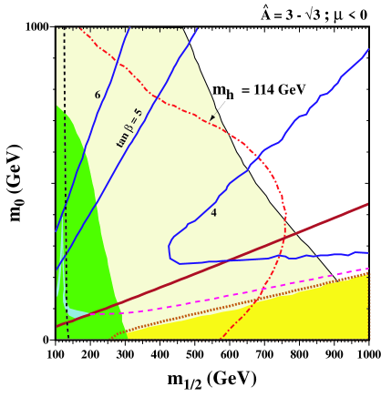
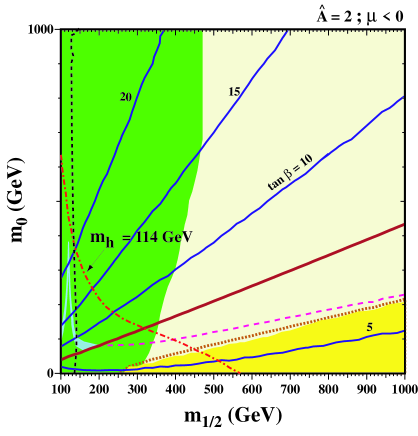
Figure 7: As in Fig. 6, but now for $\mu<0$ and the choices (a) ${\hat{A}}=3-\sqrt{3},{\hat{B}}={\hat{A}}-1$ and (b) ${\hat{A}}=2,{\hat{B}}={\hat{A}}-1$ and $\mu<0$.

6 The $\mu$ Problem and the Giudice-Masiero Mechanism

One of the primary motivations in building supersymmetric model is to avoid the the gauge hierarchy problem, namely that the Higgs mass is of order $m_{Z}$ and much less than the Planck mass, though not protected by any symmetry of the Standard Model between the GUT scale and the weak scale. Supersymmetry alleviates this problem via cancellations between contributions to the Higgs mass from fermions and bosons in the same supermultiplet. However, this scenario begs the question why supersymmetry is broken by soft terms which are assumed to be $~{}O(1~{}{\rm TeV})$. Moreover, there is one other, supersymmetric, parameter which is required to be small, namely the Higgs mixing parameter $\mu$. One of the most interesting attempts to explain the smallness of $\mu$ is the Giudice-Masiero mechanism [5], in which it is related to a coupling between observable and hidden sectors, and is of the same order of magnitude as the soft supersymmetry-breaking parameters. In the simplest realization of the Giudice-Masiero mechanism with only one hidden superfield, one has the following relation between ${\hat{A}}$ and ${\hat{B}}$, as already mentioned:

$$\hat{B}=\frac{2\hat{A}-3}{\hat{A}-3},$$ (20)

and

$$\left|\frac{\mu}{m_{0}}\right|=\left|\lambda\frac{\hat{A}-3}{\sqrt{3}}\right|$$ (21)

where $\lambda$ is the coupling constant between the hidden superfield and the two Higgs supermultiplets. One should require that $\lambda\sim O(1)$ for $\mu$ to be the same order of $m_{0}$.

We display in Fig. 8 some typical $(m_{1/2},m_{0})$ planes in the Giudice-Masiero model for positive $\mu$. As in the previous minimal supergravity VCMSSMs, we find no consistent electroweak solutions for values of ${\hat{A}}$ much outside the range of values exhibited. In the examples shown, there are no solutions above the topmost solid lines in panels (a) for ${\hat{A}}=0.6$ and (d) for ${\hat{A}}=1.8$. For $\hat{A}<-0.6$, $m_{0}\mathrel{\hbox to0.0pt{\raise 2.15277pt\hbox{$<$}\hss}{\lower 2.15277pt\hbox{$\sim$}}}150$ GeV for $m_{1/2}\leq 1000$ GeV. Similarly for $\hat{A}\mathrel{\hbox to0.0pt{\raise 2.15277pt\hbox{$>$}\hss}{\lower 2.15277pt\hbox{$\sim$}}}2.6$ only a small corner of the plane admits solutions.

In panel (a) for ${\hat{A}}=0.6$, corresponding to ${\hat{B}}=0.75$, there is no allowed region above the solid (chocolate) gravitino LSP line. Below this line, we see an allowed region for $\tan\beta\mathrel{\hbox to0.0pt{\raise 2.15277pt\hbox{$>$}\hss}{\lower 2.15277pt\hbox{$\sim$}}}22$. However, we also note that the corresponding values of $\lambda$ are quite large, $\lambda\mathrel{\hbox to0.0pt{\raise 2.15277pt\hbox{$>$}\hss}{\lower 2.15277pt\hbox{$\sim$}}}5$. The situation is somewhat different for the case ${\hat{A}}=0.8$, corresponding to ${\hat{B}}\simeq 0.64$, shown in panel (b) of Fig. 8. In this case, we see that there is a narrow allowed region along the $\chi-{\tilde{\tau}}$ coannihilation strip in the neutralino LSP region for $\tan\beta\mathrel{\hbox to0.0pt{\raise 2.15277pt\hbox{$>$}\hss}{\lower 2.15277pt\hbox{$\sim$}}}33.5$, or $\mathrel{\hbox to0.0pt{\raise 2.15277pt\hbox{$>$}\hss}{\lower 2.15277pt\hbox{$\sim$}}}35$ if the $g_{\mu}-2$ constraint is taken into account. This region requires $\lambda\mathrel{\hbox to0.0pt{\raise 2.15277pt\hbox{$>$}\hss}{\lower 2.15277pt\hbox{$\sim$}}}2$, which is relatively palatable. At lower $m_{0}$, there is a disallowed dark (red) wedge where the ${\tilde{\tau}}_{1}$ is the LSP, and below that a region where the gravitino is the LSP. The latter contains a domain allowed by the BBN/CMB decay constraint, that appears for $\tan\beta\mathrel{\hbox to0.0pt{\raise 2.15277pt\hbox{$>$}\hss}{\lower 2.15277pt\hbox{$\sim$}}}18$, or $\mathrel{\hbox to0.0pt{\raise 2.15277pt\hbox{$>$}\hss}{\lower 2.15277pt\hbox{$\sim$}}}20$ if one includes the $g_{\mu}-2$ constraint. However, this region again has $\lambda\mathrel{\hbox to0.0pt{\raise 2.15277pt\hbox{$>$}\hss}{\lower 2.15277pt\hbox{$\sim$}}}5$. Turning now to the Polonyi case ${\hat{A}}=3-\sqrt{3}$ shown in panel (c) of Fig. 8, corresponding to ${\hat{B}}\simeq 0.27$, we see that there is no allowed area in the neutralino LSP region above the dark solid (chocolate) line, and that the allowed region in the gravitino LSP region requires $\tan\beta\mathrel{\hbox to0.0pt{\raise 2.15277pt\hbox{$>$}\hss}{\lower 2.15277pt\hbox{$\sim$}}}13.5$ and again $\lambda\mathrel{\hbox to0.0pt{\raise 2.15277pt\hbox{$>$}\hss}{\lower 2.15277pt\hbox{$\sim$}}}5$. Similar features are seen in panel (d) for ${\hat{A}}=1.8$, corresponding to ${\hat{B}}=-0.5$, where the only allowed area - in the gravitino LSP region - requires even larger values of $\lambda$ than the previous cases.

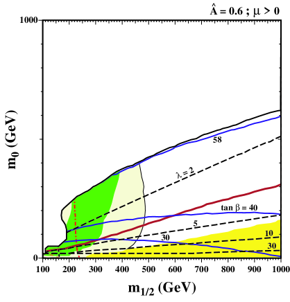
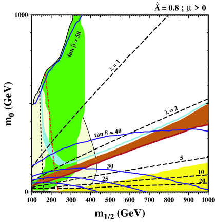
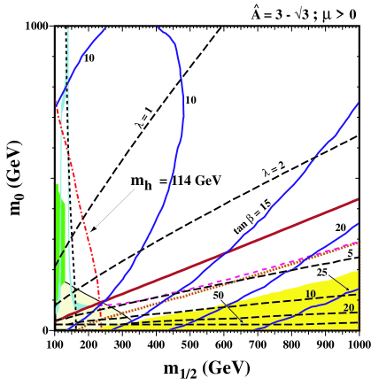
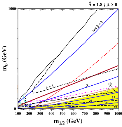
Figure 8: Examples of $(m_{1/2},m_{0})$ planes in the Giudice-Masiero model, with contours of $\tan\beta$ superposed, for $\mu>0$ and (a) ${\hat{A}}=0.6$, (b) ${\hat{A}}=0.8$, (c) ${\hat{A}}=3-\sqrt{3}$ and (d) ${\hat{A}}=1.8$. In each panel, we show the regions excluded by the LEP lower limits on MSSM particles, those ruled out by $b\to s\gamma$ decay [31] (medium, green shading), and those disfavoured by $g_{\mu}-2$ (very light, yellow shading). As before, a dotted (red) line shows where $m_{\chi}=m_{\tilde{\tau}}$ and the gravitino LSP region is bounded by a solid (chocolate) line in panels (a, c, d). The dark (red) wedge in panel (b) has a ${\tilde{\tau}}_{1}$ LSP and hence is disallowed. Within the gravitino LSP region, the relic density constraint is indicated by a dashed (pink) line and the BBN/CMB constraint on NSP decay by light (yellow) shading. The dashed black lines are contours of the Giudice-Masiero parameter $\lambda$.

Fig. 9 shows some analogous cases for $\mu<0$. As before, there are no consistent electroweak vacuum solutions for values of ${\hat{A}}$ substantially outside the range of values shown, and none above the topmost solid lines in panels (a) and (b). Panel (a) is for ${\hat{A}}=-0.2$, corresponding to ${\hat{B}}\simeq 1.06$. It has two narrow strips in the neutralino LSP region that are allowed if one discards the $g_{\mu}-2$ constraint, appearing for $m_{1/2}\mathrel{\hbox to0.0pt{\raise 2.15277pt\hbox{$>$}\hss}{\lower 2.15277pt\hbox{$\sim$}}}800$ GeV and $m_{0}\mathrel{\hbox to0.0pt{\raise 2.15277pt\hbox{$>$}\hss}{\lower 2.15277pt\hbox{$\sim$}}}500$ GeV for $\tan\beta>38$ and $\lambda<1.5$. Down in the gravitino LSP area, there is a second allowed region with $\tan\beta\mathrel{\hbox to0.0pt{\raise 2.15277pt\hbox{$<$}\hss}{\lower 2.15277pt\hbox{$\sim$}}}13$ and $\lambda\mathrel{\hbox to0.0pt{\raise 2.15277pt\hbox{$>$}\hss}{\lower 2.15277pt\hbox{$\sim$}}}3$. For smaller values of $\hat{A}$, the allowed parameter space is further squeezed. For example, for $\hat{A}=-1$ we find $m_{0}\mathrel{\hbox to0.0pt{\raise 2.15277pt\hbox{$<$}\hss}{\lower 2.15277pt\hbox{$\sim$}}}500$ GeV for $m_{1/2}\leq 1000$ GeV. In panel (b) for ${\hat{A}}=0.6$, corresponding to ${\hat{B}}=0.75$, the allowed neutralino LSP region has disappeared, but a gravitino LSP region remains. Similar features are seen in panels (c) and (d) for ${\hat{A}}=1$ (${\hat{B}}=0.5$) and ${\hat{A}}=3-\sqrt{3}$ (${\hat{B}}\simeq 0.27$), respectively. For $\hat{A}\mathrel{\hbox to0.0pt{\raise 2.15277pt\hbox{$>$}\hss}{\lower 2.15277pt\hbox{$\sim$}}}2$, solutions exist only in a small portion of the plane.

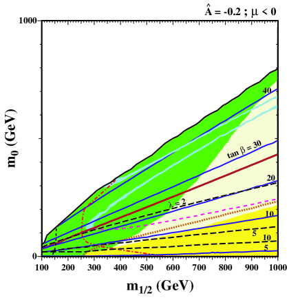
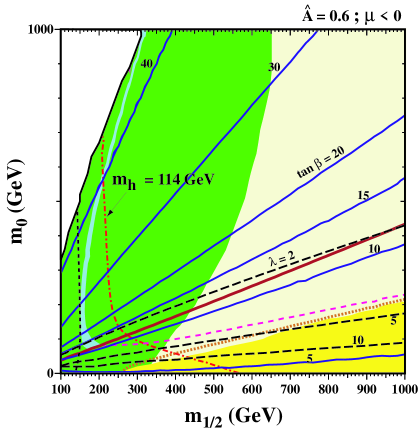
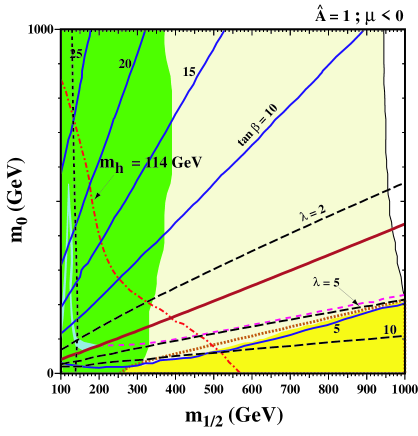
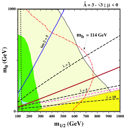
Figure 9: Same as Fig. 8, but for $\mu<0$ and (a) ${\hat{A}}=-0.2$, (b) ${\hat{A}}=0.6$, (c) ${\hat{A}}=1$, and (d) ${\hat{A}}=3-\sqrt{3}$.

7 Conclusions

We have discussed in this paper the impacts of the theoretical, experimental and cosmological constraints on some classes of VCMSSMs, including minimal supergravity models and the Giudice-Masiero model. We have presented unified treatments of the regions of parameter space in these models where the LSP is a neutralino or the gravitino.

We have emphasized that the predictions of these models differ significantly from those of the CMSSM. In particular, the CMSSM is distinct from minimal supergravity: the former does not necessarily require a fixed relation between the trilinear and bilinear soft supersymmetry-breaking parameters $A,B$, nor equality between $m_{0}$ and $m_{3/2}$, as required in minimal supergravity models. The values of $B$ required in generic realizations of the CMSSM generally bear no relation to the values that would be derived in minimal supergravity models.

In addition to minimal supergravity models, we have discussed the simplest variant of the Giudice-Masiero model, which makes a brave attempt to provide a framework for calculating the Higgs-mixing superpotential term $\mu$.

There are a couple of striking features of these specific analyses that we note. One is that the range of $A$ is often very restricted: beyond this range, it is impossible to find consistent solutions to the electroweak vacuum conditions.

A second observation is that, in both minimal supergravity and the Giudice-Masiero model, a neutralino LSP is completely excluded in many instances, and the gravitino LSP regions are generally much more extensive than the neutralino LSP regions. To some extent, this was to be expected, since we impose the cosmological dark matter density and NSP decay constraints on gravitino dark matter as one-sided upper limits, rather than as narrow WMAP ranges as for the dark matter density constraint on neutralino dark matter. This is because, in the case of gravitino dark matter, the narrow range could be reached by postulating thermal gravitino production with a suitable reheating temperature [32]. Of course, in either the neutralino or gravitino case, one could always postulate a supplementary source of cold dark matter. In the case of neutralino dark matter, this possibility would broaden the WMAP density strip down to the $m_{\chi}=m_{\tilde{\tau}}$ boundary. However, the gravitino dark matter region would still, for many choices of the other supersymmetric parameters, occupy a larger area of the $(m_{1/2},m_{0})$ plane.

In any complete supersymmetric theory, one expects some relations between supersymmetry breaking parameters, perhaps of the type discussed here. In this case, some VCMSSM should be responsible for the low-energy sparticle spectrum. However, we do not yet know what specific constraints are handed down from the unification or string scales. As we have emphasized in this paper, the predictions in such models may differ greatly from those of the more relaxed CMSSM and, a priori, those of a more general MSSM. Analogous differences are also to be expected in the predicted cross sections for direct and indirect searches for supersymmetric dark matter, a topic we will consider elsewhere.

Acknowledgments
The work of K.A.O., Y.S., and V.C.S. was supported in part by DOE grant DE–FG02–94ER–40823. Y.S. would like to thank D.A. Demir for asking about the Giudice-Maisero mechanism in this context, and for helpful conversations.

References

- [1] For reviews, see: H. P. Nilles, Phys. Rep. 110 (1984) 1; A. Brignole, L. E. Ibanez and C. Munoz, arXiv:hep-ph/9707209, published in Perspectives on Supersymmetry, ed. G. L. Kane, pp. 125-148.
- [2] H.-P. Nilles, M. Srednicki and D. Wyler, Phys. Lett. 120B (1983) 345.
- [3] J. Polonyi, Budapest preprint KFKI-1977-93 (1977).
- [4] R. Barbieri, S. Ferrara and C.A. Savoy, Phys. Lett. 119B (1982) 343.
- [5] G. F. Giudice and A. Masiero, Phys. Lett. B 206 (1988) 480.
- [6] J. R. Ellis, K. A. Olive, Y. Santoso and V. C. Spanos, Phys. Lett. B 573 (2003) 162 [arXiv:hep-ph/0305212].
- [7] M. Drees and M. M. Nojiri, Nucl. Phys. B 369 (1992) 54.
- [8] J. R. Ellis, K. A. Olive, Y. Santoso and V. C. Spanos, Phys. Lett. B 588 (2004) 7 [arXiv:hep-ph/0312262].
- [9] J. L. Feng, S. Su and F. Takayama, arXiv:hep-ph/0404231; arXiv:hep-ph/0404198; J. L. Feng, A. Rajaraman and F. Takayama, Phys. Rev. Lett. 91 (2003) 011302 [arXiv:hep-ph/0302215].
- [10] R. H. Cyburt, J. R. Ellis, B. D. Fields and K. A. Olive, Phys. Rev. D 67 (2003) 103521 [arXiv:astro-ph/0211258].
- [11] K. Jedamzik, arXiv:astro-ph/0402344; M. Kawasaki, K. Kohri and T. Moroi, arXiv:astro-ph/0402490.
- [12] R. Arnowitt and P. Nath, Phys. Rev. D 46 (1992) 3981; V. D. Barger, M. S. Berger and P. Ohmann, Phys. Rev. D 49 (1994) 4908 [arXiv:hep-ph/9311269].
- [13] W. de Boer, R. Ehret and D. I. Kazakov, Z. Phys. C 67 (1995) 647 [arXiv:hep-ph/9405342]; D. M. Pierce, J. A. Bagger, K. T. Matchev and R. J. Zhang, Nucl. Phys. B 491 (1997) 3 [arXiv:hep-ph/9606211].
- [14] M. Carena, J. R. Ellis, A. Pilaftsis and C. E. Wagner, Nucl. Phys. B 625 (2002) 345 [arXiv:hep-ph/0111245].
- [15] CDF Collaboration, D0 Collaboration and Tevatron Electroweak Working Group arXiv:hep-ex/0404010.
- [16] M. Battaglia et al., Eur. Phys. J. C 22 (2001) 535 [arXiv:hep-ph/0106204].
- [17] H. Baer, F. E. Paige, S. D. Protopopescu and X. Tata, ISAJET 7.48: A Monte Carlo event generator for , , and reactions, hep-ph/0001086. The latest update is available from http://paige.home.cern.ch/paige/.
- [18] J. Tabei and H. Hotta, arXiv:hep-ph/0208039.
- [19] J. R. Ellis, K. A. Olive, Y. Santoso and V. C. Spanos, Phys. Lett. B 565 (2003) 176 [arXiv:hep-ph/0303043].
- [20] U. Chattopadhyay, A. Corsetti and P. Nath, Phys. Rev. D 68 (2003) 035005 [arXiv:hep-ph/0303201]; H. Baer and C. Balazs, JCAP 0305, 006 (2003) [arXiv:hep-ph/0303114]; A. B. Lahanas and D. V. Nanopoulos, Phys. Lett. B 568, 55 (2003) [arXiv:hep-ph/0303130]; R. Arnowitt, B. Dutta and B. Hu, arXiv:hep-ph/0310103.
- [21] C. L. Bennett et al., arXiv:astro-ph/0302207; D. N. Spergel et al., arXiv:astro-ph/0302209.
- [22] J. R. Ellis, S. Heinemeyer, K. A. Olive and G. Weiglein, Phys. Lett. B 515 (2001) 348 [arXiv:hep-ph/0105061].
- [23] J. L. Feng, K. T. Matchev and T. Moroi, Phys. Rev. D 61 (2000) 075005 [arXiv:hep-ph/9909334]; A. Romanino and A. Strumia, Phys. Lett. B 487 (2000) 165 [arXiv:hep-ph/9912301].
- [24] G. W. Bennett et al. [Muon g-2 Collaboration], Phys. Rev. Lett. 92 (2004) 161802 [arXiv:hep-ex/0401008].
- [25] M. Davier, S. Eidelman, A. Hocker and Z. Zhang, Eur. Phys. J. C 31 (2003) 503 [arXiv:hep-ph/0308213].
- [26] K. Hagiwara, A. D. Martin, D. Nomura and T. Teubner, arXiv:hep-ph/0312250.
- [27] J. F. de Trocóniz and F. J. Ynduráin, arXiv:hep-ph/0402285.
- [28] K. Melnikov and A. Vainshtein, arXiv:hep-ph/0312226.
- [29] D. Acosta et al. [CDF Collaboration], arXiv:hep-ex/0403032.
- [30] D. M. Pierce, J. A. Bagger, K. T. Matchev and R. j. Zhang, Nucl. Phys. B 491 (1997) 3 [arXiv:hep-ph/9606211].
- [31] M.S. Alam et al., [CLEO Collaboration], Phys. Rev. Lett. 74 (1995) 2885 as updated in S. Ahmed et al., CLEO CONF 99-10; BELLE Collaboration, BELLE-CONF-0003, contribution to the 30th International conference on High-Energy Physics, Osaka, 2000. See also K. Abe et al., [Belle Collaboration], [arXiv:hep-ex/0107065]; L. Lista [BaBar Collaboration], [arXiv:hep-ex/0110010]; C. Degrassi, P. Gambino and G. F. Giudice, JHEP 0012 (2000) 009 [arXiv:hep-ph/0009337]; M. Carena, D. Garcia, U. Nierste and C. E. Wagner, Phys. Lett. B 499 (2001) 141 [arXiv:hep-ph/0010003]; P. Gambino and M. Misiak, Nucl. Phys. B 611 (2001) 338; D. A. Demir and K. A. Olive, Phys. Rev. D 65 (2002) 034007 [arXiv:hep-ph/0107329]; T. Hurth, arXiv:hep-ph/0212304.
- [32] M. Bolz, A. Brandenburg and W. Buchmuller, Nucl. Phys. B 606 (2001) 518 [arXiv:hep-ph/0012052]; W. Buchmuller, K. Hamaguchi and M. Ratz, Phys. Lett. B 574 (2003) 156 [arXiv:hep-ph/0307181].