Efficient solar anti-neutrino production in random magnetic fields

Abstract:

We have shown that the electron anti-neutrino appearance in the framework of the spin flavor conversion mechanism is much more efficient in the case of neutrino propagation through random than regular magnetic field. This result leads to much stronger limits on the product of the neutrino transition magnetic moment and the solar magnetic field based on the recent KamLAND data. We argue that the existence of the random magnetic fields in the solar convective zone is a natural sequence of the convective zone magnetic field evolution.

1 Introduction

Recently the KamLAND experiment has announced that the electron anti-neutrino component in the solar flux is less than $2.8\times 10^{-2}\%$ of the solar boron flux at the $90\%$ C.L. [1], a bound about 30 times more stringent than the latest Super-Kamiokande limit [2].

The presence of electron anti-neutrinos in the solar flux may indicate the existence of spin-flavor precession (SFP) induced by non-vanishing neutrino transition magnetic moments [3, 4] interacting with solar magnetic fields or, alternatively, neutrino decays in models with spontaneous violation of lepton number [5, 6, 7]. Here we discuss the case of anti-neutrinos produced by SFP conversions.

The first KamLAND evidence of reactor anti-neutrino disappearance [8] had already excluded SFP scenarios as solutions to the solar neutrino problem [9]. Together with the latest KamLAND limit on the solar electron anti-neutrino flux [1] and including the recent SNO salt results [10] the robustness of the LMA MSW solution to the solar neutrino problem (SNP) against the SFP mechanism was confirmed [13]. However, a neutrino magnetic moment could still play a notable role and lead to sub-leading, but potentially observable, effects.

To analyze the SFP conversion several solar magnetic field models were considered previously, characterized by different assumptions pertaining to their magnitude, location and typical scales, regular or random nature [14, 15, 16, 17, 18] coming from our lack of knowledge about solar magnetic fields. Usually the solar magnetic fields are supposed to reside within the solar convective zone [14, 15, 16] in agreement with dynamo mechanism. Sometimes they are considered to be located in the solar core or in the radiative zone [17, 18]. Although allowed, these are not physically as persuasive as the former ones.

In what follows we adopt the conservative point of view, assuming a convective zone magnetic field model and exploiting the fact that in accordance with the present-day understanding of solar magnetic field evolution, the large-scale magnetic field in the solar convective zone is followed by a small-scale random component, the strength of which is comparable to or even larger than that of the regular one.

The main issue we advocate here is that within the SFP scenario, solar random magnetic fields can generally result in a sizable gain in electron anti-neutrino yield, up to one-two orders of magnitude as compared to regular fields of the same (in the average) amplitude. This results in more stringent limits on the product of the neutrino magnetic moment and magnetic field strength, $\mu_{\nu}B$.

2 Neutrinos in random magnetic fields

Let us consider, for simplicity, the spin flavour precession of two Majorana neutrinos in vacuum  [3]. The evolution of the system is governed by the Schrödinger-like equation

$$i\>{\vec{\nu}}={\cal H}\>\vec{\nu},$$ (1)

where $\vec{\nu}^{T}=(\nu_{1},\bar{\nu}_{2})$, $\nu_{i}$ are neutrino mass states,

$${\cal H}=\mu_{\nu}B_{x}\>\sigma_{1}-\mu_{\nu}B_{y}\>\sigma_{2}-\delta\cdot\sigma_{3}$$ (2)

is the $(2\times 2)$ Hamiltonian, $\sigma_{j}$ – Pauli matrices, $\mu_{\nu}$ – the neutrino transition magnetic moment, $B_{x}$ and $B_{y}$ are magnetic field components perpendicular to the neutrino trajectory (along $z$ axis), and $\delta=\Delta m^{2}/4E$; $E$ and $\Delta m^{2}$ are the neutrino energy and the squared mass difference, respectively.

In a uniform magnetic field the conversion probability is

$$P\left(\nu_{1}\to\bar{\nu}_{2};L\right)=\frac{\mu^{2}_{\nu}B^{2}_{\perp}}{\delta^{2}+\mu^{2}_{\nu}B^{2}_{\perp}}\sin^{2}\left(\sqrt{\delta^{2}+\mu^{2}_{\nu}B^{2}_{\perp}}L\right),$$ (3)

where $L$ is the neutrino path in the magnetic field region. Hereafter we will not distinguish $z$ and $t$ assuming $z=t$ for $c=1$.

Let us now assume that a probe neutrino crosses a region with a small-scale random magnetic field with effective scale $L_{0}$. The neutrino trajectory is divided into about $N=L/L_{0}$ correlation cells. For a given realization, the random magnetic field vector is assumed to be uniform within each cell; the fields in adjacent cells are uncorrelated and, moreover, within one cell different magnetic field components, transversal to the neutrino trajectory, are also independent random (Gaussian) variables with zero mean value [14].

In the uniform magnetic field case the evolution matrix $U=\exp\{-i{\cal H}\cdot z\}$ is trivially found. For any piece-constant magnetic field profile (set of field domains) it is then just the product of corresponding unitary matrices,

$$U(L)=\prod^{N}_{j=1}U_{j},$$ (4)

where

$$U_{j}=\exp(-i{\cal H}L_{0})=\cos\omega_{j}-i(\vec{\sigma}\cdot\vec{n_{j}})\sin\omega_{j}$$ (5)

with

$$\begin{array}[]{cc}\omega_{j}={\cal D}_{j}\cdot L_{0},&{\cal D}_{j}=\sqrt{\delta^{2}+\mu^{2}B^{2}_{j\perp}},\\ \vec{n}_{j}=(\mu_{\nu}B_{jx},-\mu_{\nu}B_{jy},-\delta)\cdot{\cal D}_{j}^{-1}&\vec{n}^{2}_{j}=1.\end{array}$$ (6)

The neutrino conversion probability after crossing the random magnetic field region is therefore equal to the corresponding matrix element,

$$P(\nu_{1}\to\bar{\nu}_{2};L)=\langle 0|U_{1}^{*}U_{2}^{*}...U_{N}^{*}\frac{1-\sigma_{3}}{2}U_{N}...U_{2}U_{1}|0\rangle,$$ (7)

where $|0\rangle^{T}=(1,0)$ is the initial neutrino state and $(1-\sigma_{3})/2={\rm diag}(0,1)$ is the projector on to $\bar{\nu}_{2}$ state. Because of the multiplicative nature of the evolution matrix, Eq.(4), we perform the averaging of the conversion probability step by step. After commutation we obtain the following inner matrix structure

$$U_{N}^{*}\frac{1-\sigma_{3}}{2}U_{N}=\frac{1}{2}[1-\cos(2\omega_{N})\cdot\sigma_{3}-\sin(2\omega_{N})\cdot[\vec{n}_{N}\times\vec{\sigma}]_{3}-2\sin^{2}\omega_{N}\cdot n_{N,3}(\vec{\sigma}\vec{n}_{N})].$$ (8)

Taking into account that averaging over random magnetic fields in the $N$-th cell washes out all terms proportional to odd powers of $B_{x}^{(N)}$ and $B_{y}^{(N)}$, we obtain

$$\left\langle U^{*}_{N}\frac{1-\sigma_{3}}{2}U_{N}\right\rangle_{\mbox{av}}=\frac{1}{2}\left[1-\left(1-2\left\langle\left(1-n^{2}_{N,3}\right)\sin^{2}\omega_{N}\right\rangle_{\mbox{av}}\right)\sigma_{3}\right],$$ (9)

that is just the same diagonal matrix as the initial projection operator modified only by a scalar factor in front of $\sigma_{3}$.

Therefore by induction and after some algebra we obtain

$$\left\langle P(\nu_{1}\to\bar{\nu}_{2};L)\right\rangle_{\mbox{av}}=\frac{1}{2}-\frac{1}{2}\prod^{N}_{j=1}\left(1-2P_{j}^{(c)}\right),$$ (10)

where $P_{j}^{(c)}$ is the averaged conversion (flavour-changing) probability in the j-th correlation cell given by

$$P_{j}^{(c)}=\left\langle\frac{\mu^{2}_{\nu}B^{2}_{j\perp}}{\delta^{2}+\mu_{\nu}^{2}B^{2}_{j\perp}}\sin^{2}\left(\sqrt{\delta^{2}+\mu^{2}_{\nu}B^{2}_{j\perp}}L_{0}\right)\right\rangle_{\mbox{av}}.$$ (11)

When all conversion probabilities are small, i.e. when $\mu^{2}_{\nu}\left\langle B^{2}_{\perp}\right\rangle\ll\delta^{2}$ (and this is the case for solar neutrino oscillation parameters and realistic magnetic fields, see below), Eq.(10) is greatly simplified,

$$\left\langle P(\nu_{1}\to\bar{\nu}_{2};L)\right\rangle_{\mbox{av}}\approx\sum^{N}_{j=1}P_{j}^{(c)}=\sum^{N}_{j=1}\frac{\mu^{2}_{\nu}\left\langle B^{2}_{j\perp}\right\rangle}{\delta^{2}}\sin^{2}\left(\delta\cdot L_{0}\right).$$ (12)

The above results mean that because of the randomness of magnetic fields the neutrino spin-flavour evolution looses coherence, that is instead of dealing with wave functions it is necessary to consider probabilities. Therefore for small conversion the resulting effect is of cumulative nature and the probability is proportional to the number of correlation cells of the random magnetic field.

Let’s assume that all root-mean-square random field amplitudes in different cells are equal to the strength of some constant regular magnetic field. In this case we see that the above result is proportional to the number of correlation cells traversed by neutrino, $N=L/L_{0}$, thus leading to a sizable gain in neutrino conversion in random field as compared with the case of a constant magnetic field of the same amplitude. Indeed, in the case of regular field from Eq.(3) we have

$$P(\nu_{1}\to\bar{\nu}_{2};L)\approx\frac{\mu_{\nu}^{2}B_{\perp}^{2}}{\delta^{2}}\sin^{2}\left(\delta L\right)+O\left(\left(\frac{\mu_{\nu}^{2}B_{\perp}^{2}}{\delta^{2}}\right)^{2}\right)\approx\frac{\mu_{\nu}^{2}B_{\perp}^{2}}{2\delta^{2}}~{},$$ (13)

that is similar to the case of neutrino passing only one cell of the size $L$.

3 Neutrinos in solar random magnetic fields

The simplified approach given above can be taken over to the general case of the neutrino spin flavour precession in solar random magnetic fields [13]. Within this generalized picture (LMA-MSW + SFP), after the MSW flavour conversion occurred in the inner region of the Sun, $\bar{\nu}_{e}$’s are produced due to the magnetic moment conversion $\nu_{\mu}\to\bar{\nu}_{e}$ in the convective zone magnetic field. The two-flavour Majorana neutrino evolution Hamiltonian in matter and magnetic field is well–known to be four–dimensional [3, 4]. However for solar convective zone random magnetic fields the full $4\times 4$ evolution equation decouples into two $2\times 2$ equations describing LMA-MSW oscillations deep in the Sun and the following (approximate) vacuum SFP conversions inside the solar convective zone [13]. This is explained by smallness of two main parameters, $V/\delta\simeq 10^{-2}$ , where $V$ is the matter potential within the convective zone, and

$$\kappa=\frac{\mu_{\nu}^{2}b_{\perp}^{2}}{\delta^{2}}=2.5\times 10^{-5}\left(\frac{\mu_{\nu}}{10^{-11}\mu_{B}}\right)^{2}\left(\frac{b_{\perp max}}{100{\rm kG}}\right)^{2}\left(\frac{7\times 10^{-5}{\rm eV^{2}}}{\Delta m^{2}}\right)^{2}\left(\frac{E}{10{\rm MeV}}\right)^{2}~{}.$$ (14)

The first parameter tells us that the matter effects inside the convective zone are negligible and can be safely neglected. The smallness of the parameter $\kappa$ allows to use the perturbative approach described in Section 2.

4 Results and Discussion

From the above discussion one sees that spin flavor conversion is much more efficient in producing solar anti-neutrinos for random magnetic fields than for the case of regular fields. To confirm our conclusions numerically we compute the limits on $\mu_{\nu}B$ both for regular and for random magnetic fields. The results are plotted in Fig. 1.

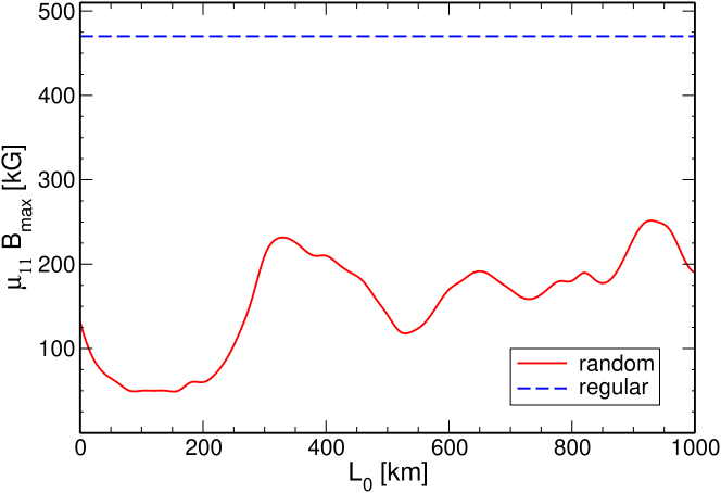
Figure 1: Bounds on $\mu_{11}B_{max}$ for random magnetic field versus correlation scale $L_{0}$ (solid line). The horizontal dashed line indicates the bound on $\mu_{11}B_{max}$ for Kutvitsky-Solov’ev regular magnetic field. $\mu_{11}$ is magnetic moment in units of $10^{-11}$ Bohr magneton. Details are given in text.

The full available set of neutrino data was taken into account along with recent KamLAND bound on the electron anti-neutrino flux [1]. To make connection with previous results the Kutvitsky-Solov’ev magnetic field [9, 15] was taken as a reference regular field as well as the root-mean-square random field shape. Here the correlation scale $L_{0}$ was considered as an additional free parameter. For regular fields we obtain the constraint

$$\mu_{\nu}B_{max}<10^{-11}\mu_{B}\times 470~{}\mbox{kG at 90\% C.L.}$$

On the other hand for the random magnetic field case one finds, in the most conservative case,

$$\mu_{\nu}B_{max}<10^{-11}\mu_{B}\times 250~{}\mbox{kG at $L_{0}\sim 950$~{}km (90\% C.L)}$$

while for the most optimistic case

$$\mu_{\nu}B_{max}<10^{-11}\mu_{B}\times 50~{}\mbox{kG at $L_{0}\sim 100$~{}km (90\% C.L).}$$

If we further specify the random magnetic field model to be of the turbulent type one can eliminate a dependence upon the correlation scale since neutrinos effectively feel only one scale with the space period equal to the neutrino oscillation length [13].

Taking into account that the present-day understanding of the solar magnetic field evolution leads to small-scale convective zone random magnetic fields comparable or even exceeding the large-scale ones, we can conclude that the former indeed can play an important role in the analysis of the solar neutrino data.

- [1] KamLAND, K. Eguchi et al., Phys. Rev. Lett. 92, 071301 (2004), [hep-ex/0310047].
- [2] Super-Kamiokande, Y. Gando et al., Phys. Rev. Lett. 90, 171302 (2003), [hep-ex/0212067].
- [3] J. Schechter and J. W. F. Valle, Phys. Rev. D24, 1883 (1981), Err. Phys. Rev. D25, 283 (1982).
- [4] E. K. Akhmedov, Phys. Lett. B213, 64 (1988). C.-S. Lim and W. J. Marciano, Phys. Rev. D37, 1368 (1988).
- [5] J. Schechter and J. W. F. Valle, Phys. Rev. D25, 774 (1982).
- [6] J. W. F. Valle, Phys. Lett. B 131 (1983) 87. G. B. Gelmini and J. W. F. Valle, Phys. Lett. B142, 181 (1984). M. C. Gonzalez-Garcia and J. W. F. Valle, Phys. Lett. B216, 360 (1989).
- [7] J. F. Beacom and N. F. Bell, Phys. Rev. D65, 113009 (2002), [hep-ph/0204111].
- [8] KamLAND, K. Eguchi et al., Phys. Rev. Lett. 90, 021802 (2003), [hep-ex/0212021].
- [9] J. Barranco, O. G. Miranda, T. I. Rashba, V. B. Semikoz and J. W. F. Valle, Phys. Rev. D66, 093009 (2002), [hep-ph/0207326 v3 KamLAND-updated version].
- [10] SNO, S. N. Ahmed et al., Phys. Rev. Lett. , 041801 (2003), [nucl-ex/0309004].
- [11] M. Maltoni, T. Schwetz, M. A. Tortola and J. W. F. Valle, Phys. Rev. D68, 113010 (2003), [hep-ph/0309130].
- [12] M. Maltoni, T. Schwetz and J. W. F. Valle, Phys. Rev. D67, 093003 (2003), [hep-ph/0212129].
- [13] O. G. Miranda, T. I. Rashba, A. I. Rez and J. W. F. Valle, hep-ph/0311014.
- [14] A. A. Bykov, V. Y. Popov, A. I. Rez, V. B. Semikoz and D. D. Sokoloff, Phys. Rev. D59, 063001 (1999), [hep-ph/9808342].
- [15] V. A. Kutvitskii and L. S. Solov’ev, J. Exp. Theor. Phys. 78, 456 (1994).
- [16] M. M. Guzzo and H. Nunokawa, Astropart. Phys. 12, 87 (1999), [hep-ph/9810408].
- [17] E. K. Akhmedov and J. Pulido, Phys. Lett. B553, 7 (2003), [hep-ph/0209192].
- [18] A. Friedland and A. Gruzinov, Astropart. Phys. 19, 575 (2003), [hep-ph/0202095].