Loop integration results using numerical extrapolation for a non-scalar integral

Abstract

Loop integration results have been obtained using numerical integration and extrapolation. An extrapolation to the limit is performed with respect to a parameter in the integrand which tends to zero. Results are given for a non-scalar four-point diagram. Extensions to accommodate loop integration by existing integration packages are also discussed. These include: using previously generated partitions of the domain and roundoff error guards.

Keywords. One-loop correction, non-scalar four-point function, numerical integration, extrapolation.

1 INTRODUCTION AND BACKGROUND

In a general form, loop integrals used for cross section corrections are given by

$${\mathcal{I}}[\wp]=\int\prod_{\lambda=1}^{L}\frac{\mathrm{d}^{4}l_{\lambda}}{{(2\pi)}^{4}i}\prod_{\ell=1}^{N}\frac{{\wp}(k_{1},\ldots,k_{N})}{k_{\ell}^{2}-m_{\ell}^{2}+i\varepsilon},$$ (1)

where $N$ is the number of propagators, $L$ the number of loops, the momentum on the $\ell$-th internal line is $k_{\ell}$ and the corresponding mass is $m_{\ell},$$1\leq\ell\leq N.$

As a special case, scalar one-loop integrals of the form $(-1)^{n}/(16\pi^{2})I_{n}$ where

I_n = ∫_S_n-1 1(Dn(x)-iε)n-2 dx

(2)

are obtained from (1) by introducing Feynman parameters and integrating over the loop momentum $l$. The integration region $S_{n-1}$ is the $n-1$ dimensional unit simplex.

For the simplest cases, the results can be obtained analytically. Numerical techniques have been successful with considerable analytic manipulation (see, e.g., [1, 2]). In previous work [3], we reported results for integrals of the form (2) treated numerically using extrapolation by the $\varepsilon$-algorithm [4]. We will now consider the case of a one-loop integral where the numerator in the integrand is a polynomial of the Feynman parameters. A sample problem involving the $e^{-}e^{+}\rightarrow W^{-}~{}W^{+}$ interaction is given in the next section of this paper. Results for this problem are given in Section 3. Section 4 discusses enhancements to the ParInt parallel integration package.

2 NON-SCALAR INTEGRAL

The matrix element of one-loop corrections is given by the real part of the product of a one-loop amplitude and the (conjugate of) a tree amplitude. Figure 1 shows an example of a box diagram and a tree diagram of a $Z$-boson exchange for the interaction $e^{-}e^{+}\rightarrow W^{-}~{}W^{+}.$ The Feynman diagram and the corresponding matrix element are generated automatically by GRACE-loop[5] system.

After introducing the Feynman parameters as in Figure 1, and integrating over the loop momentum, the matrix element is of the following form,

$$M_{4}(f,g;\varepsilon)=\int dxdydz\left[\frac{f(x,y,z)}{(D_{4}-i\varepsilon)^{2}}-2\frac{g(x,y,z)}{D_{4}-i\varepsilon}\right]$$

where $D_{4}={~{}}^{\tau}{\bf x}A{\bf x}+2{\bf v}\cdot{\bf x}+C,$ and $A_{\iota j}=q_{\iota}\cdot q_{j},~{}q_{1}=-p_{e^{-}},~{}q_{2}=p_{e^{+}},~{}q_{3}=p_{e^{+}}-p_{W^{+}}$, $C=M_{0}^{2}=M_{Z}^{2}$, $v_{\iota}=\frac{1}{2}(-q_{\iota}^{2}+M_{\iota}^{2}-M_{0}^{2})$ with $M_{1}=m_{e},M_{2}=M_{W},M_{3}=m_{e}$.

Figure 1: Feynman diagram for $e^{-}e^{+}\rightarrow W^{-}~{}W^{+}$

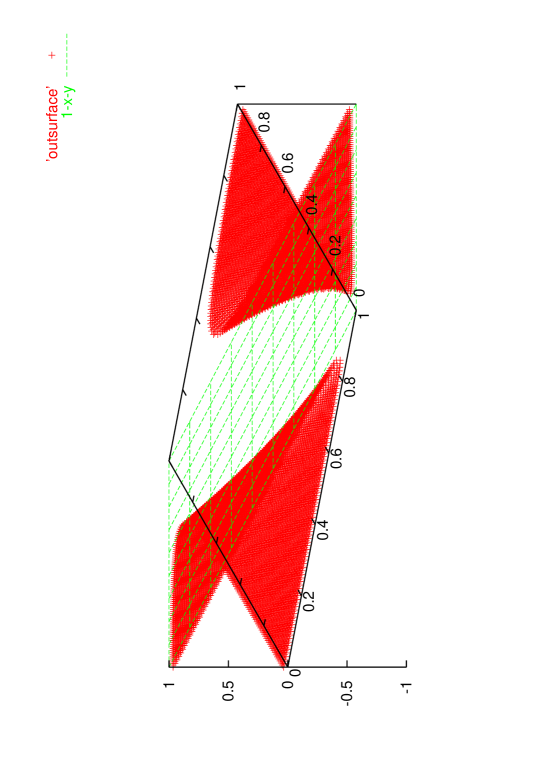
Figure 2 shows the $D_{4}=0$ surface of the singularity over $-1\leq x,y\leq 1,$ and delineates the integration domain ${\mathcal{S}}_{3}.$

$f$ and $g$ are polynomials of Feynman parameters, of which the coefficients are determined by external momenta and masses of internal lines. Here $M_{Z}=91.187{\rm GeV},M_{W}=80.22{\rm GeV},m_{e}=0.511{\rm MeV},~{}\sqrt{s}=500~{}{\rm GeV}$  and  $\theta=\angle({\bf p}_{e^{-}},{\bf p}_{W^{-}})$. The numerical results are evaluated for $\cos\theta=0.956811390.$

The generalized non-linear gauges[5] are implemented for the amplitude. The result depends on the gauge parameters because only one diagram is picked up. For the numerical evaluation, the non-linear gauge parameters are set as $\tilde{\alpha}=2,\tilde{\beta}=3,\tilde{\delta}=4,\tilde{\epsilon}=5$ and $\tilde{\kappa}=6$.

3 GRAPH 216 RESULTS

Table 1 illustrates the use of the $\varepsilon$-algorithm for the integral computation of the term involving $f$ (the symbolic code of which has about 2000 lines as FORTRAN code). We show the results of the extrapolation for the real part of $M_{4}(f,0;\varepsilon).$ The method is based on generating a sequence of integral values corresponding to a geometric sequence of $\varepsilon$ and extrapolating to the limit as $\varepsilon\rightarrow 0.$

Figure 2: $D_{4}=0$ surface

The table shows the sequence of integral approximations for $\varepsilon=1.2^{30-\ell},~{}~{}\ell=0,1,\ldots$ (obtained numerically) in the first (leftmost) column. Using the integral approximations corresponding to $\ell=0,1,2,$ the first extrapolated result is obtained (top element of column 2). Using the $\ell=3$ element of column 1, the second extrapolated result is obtained in column 2; the $\ell=4$ element of column 1 is then used to generate the third element of column 2 and the top element of column 3. In all iterations following, the new element in column 1 is used to generate a new lower diagonal of the triangular table.

The table elements are shown to 8-digit accuracy, which is the final accuracy obtained in this run. Convergence is apparent down the columns and along the lower diagonal. Relying on a heuristic error estimate of the table elements along the lower diagonal, an element is selected as the result (printed boldface). The result calculated analytically is -0.647837287.

Table 1: Extrapolation table for the real part of $M_{4}(f,0;\varepsilon)$

$\ell$
0	-0.65001198
1	-0.65102708	-0.65168630
2	-0.65142675	-0.65143432	-0.64911741
3	-0.65143418	-0.65142699	-0.64873688	-0.64669569
4	-0.65121543	-0.65186148	-0.64837272	-0.64766170	-0.64787059
5	-0.65088469	-0.65400251	-0.64811405	-0.64780004	-0.64784821	-0.64784032
6	-0.65051471	-0.61144371	-0.64796871	-0.64783212	-0.64784301	-0.64784011	-0.64784042
7	-0.65014820	-0.64536958	-0.64789843	-0.64783979	-0.64784142	-0.64783917	-0.64783494	-0.64783735
8	-0.64980779	-0.64694643	-0.64786686	-0.64784110	-0.64784083	-0.64783800	-0.64783707	-0.64783723	-0.647837056
9	-0.64950358	-0.64742949	-0.64785289	-0.64784075	-0.64784147	-0.64783737	-0.64783720	-0.64783719
10	-0.64923827	-0.64763299	-0.64784650	-0.64784000	-0.64782758	-0.64783723	-0.64783718
11	-0.64901060	-0.64773083	-0.64784332	-0.64783920	-0.64783650	-0.64783719
12	-0.64881731	-0.64778110	-0.64784155	-0.64783848	-0.64783702
13	-0.64865441	-0.64780784	-0.64784045	-0.64783791
14	-0.64851780	-0.64782228	-0.64783970
15	-0.64840361	-0.64783009
16	-0.64830839

To generate the integral approximation in the first column, we used an iterated integration where the adaptive Quadpack [6] routine dqage was used in each direction, requesting a relative accuracy of $10^{-10}.$ So far, this technique has outperformed other numerical integration approaches using multivariate (cubature) rules.

4 PARINT ENHANCEMENTS

ParInt is a software package for parallel multivariate integration [7]. It has components for multivariate integration using Monte Carlo (mc), Quasi-Monte Carlo (qmc) and adaptive methods. ParInt is written in C and runs over MPI [8] on a distributed platform.

4.1 Iterated integration

While the adaptive approach could not be applied directly using 3D multivariate rules, results to 6-figure accuracy were obtained by treating the problem as a 2D integration of a 1D integral. The 1D inner integral was calculated with Quadpack routine dqage.

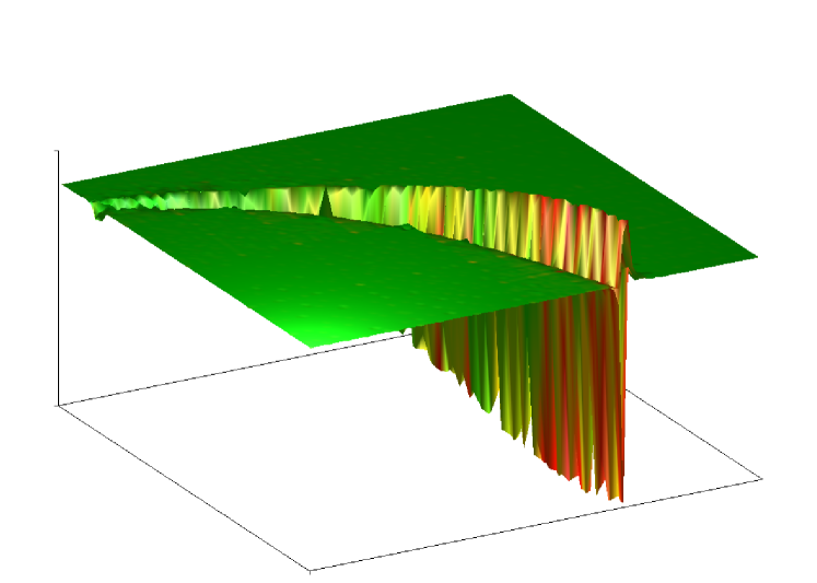
The 2D integration was performed with ParInt and with its Fortran sequential predecessor, dcuhre [9]. The local region error estimate was changed to make it less conservative. Figure 3 illustrates the integrand of the 2D problem for $\varepsilon=1.2^{25},$ which was drawn using evaluation points of the integration. We are currently considering a design of ParInt which will allow incorporating iterated integration in a transparent way.

Figure 3: 2D of 1D integrand for Graph 216 real part

It recently came to our attention that in the work by Binoth, Heinrich and Kauer [10], 3D box integrals are obtained by performing the inner integration analytically, which leaves the resulting 2D integrand with an integrable (though still problematic) singularity. Note further that their 3D box together with 2D vertex diagram evaluations are at the basis of reductions performed to treat scalar hexagon integrals.

4.2 Re-use of subregions between extrapolations

A sequence of extrapolation steps uses a series of similar integrations which share similar subregions when performed adaptively. At each step of the extrapolation, ParInt can avoid a significant number of region evaluations by re-using previously “discovered” subregions as the initial set of regions for the next extrapolation step, potentially avoiding a significant amount of computation.

ParInt has been modified to support this activity by storing the active integration regions at the end of every parallel run and providing the user with the option to load a set of regions to initialize a run. Regions may be saved either locally on each compute node or in a single file managed by the controller. Regions loaded at the start of a subsequent computation may also be read from a single global file or individual files on each compute node. We are currently developing a distributed I/O system which will allow compute nodes to retrieve previously saved regions from files on any other compute node [11].

4.3 Kahan summation

The global adaptive integration algorithm first developed by De Ridder and Van Dooren [12] is also used by ParInt. At each step, one region (per worker) is selected and subdivided into subregions. The selected integration rule is applied over each subregion. Next, the estimated error and result for the selected region and subregions must be subtracted from and added to the total estimated error and result, respectively. For difficult problems, ParInt will select many regions and subdivide them. Numerical summation of millions of terms can introduce round off error and greatly reduce the accuracy of the result and estimated error in a numerical integration routine.

We have looked at several techniques to reduce round off error in sums with a large number of terms. Each of these techniques has its own merits and flaws. A good method would be one whose accuracy does not depend on the number of terms in the sum and would not greatly impact the runtime performance of a numerical integration routine. A compensated summation method developed by W. Kahan [13] and further studied by N. Higham [14] best fits these needs. Several advantages of this method are low computational overhead, low storage requirements, and in error analysis it is shown to have an error constant of order 1.

5 CONCLUSIONS

We presented results for a non-scalar one-loop box diagram, where the integral is obtained using numerical integration and extrapolation with the $\varepsilon$-algorithm. We described enhancements to the ParInt parallel integration package, which are in various stages of development. Furthermore, in future work, we plan to investigate combinations of our numerical methods with symbolic techniques.

References

- [1] Fujimoto, J., Shimizu, Y., Kato, K., and Oyanagi, Y. Progress of Theoretical Physics 87, 5 (1992), 1233–1247
- [2] Ferroglia, A., Passera, A, Passarino, G, and Uccirati, S, Nucl. Phys. B 650 (2003) 162 [arXiv:hep-ph/0209219].
- [3] de Doncker, E., Shimizu, Y., Fujimoto, J., and Yuasa, F. Computer Physics Communications (2004). Accepted.
- [4] Wynn, P. Mathematical Tables and Aids to Computing 10 (1956), 91–96.
- [5] Bélanger, G., Boudjema, F., Fujimoto, J., Ishikawa, T., Kaneko, T., and Shimizu, Y. hep-ph/0308080.
- [6] Piessens, R., de Doncker, E., Überhuber, C. W., and Kahaner, D. K. Springer Series in Computational Mathematics. Springer-Verlag, 1983.
- [7] http://www.cs.wmich.edu/parint, ParInt web site.
- [8] http://www-unix.mcs.anl.gov/mpi/index.html, MPI web site.
- [9] Berntsen, J., Espelid, T. O., and Genz, A. ACM Trans. Math. Softw. 17 (1991), 437–451.
- [10] Binoth, T., Heinrich, G., and Kauer, N. hep-ph/0210023.
- [11] Cucos, L. PhD dissertation, Western Michigan University, Nov. 2003.
- [12] De Ridder, L., and Van Dooren, P. Journal of Computational and Applied Mathematics 2, 3 (1976), 207–210.
- [13] Kahan, W. Comm. ACM 8 (1965), 40.
- [14] Higham, N. J. SIAM J. Sci. Comput. 14, 4 (July 1993), 783–799.