CP violation in the partial width asymmetries for $B^{-}\to\pi^{+}\pi^{-}K^{-}$ and $B^{-}\to K^{+}K^{-}K^{-}$ decays
S. Fajfer^a,b, T.N. Pham^c and A. Prapotnik^a

a) J. Stefan Institute, Jamova 39, P. O. Box 3000, 1001 Ljubljana, Slovenia

b) Department of Physics, University of Ljubljana, Jadranska 19, 1000 Ljubljana, Slovenia

c) Centre de Physique Theorique, Centre National de la Recherche Scientifique, UMR 7644, Ecole Polytechnique, 91128 Palaiseau Cedex, France

ABSTRACT

We investigate a possibility of observing CP asymmetries in the partial widths for the decays $B^{-}\to\pi^{+}\pi^{-}K^{-}$ and $B^{-}\to K^{+}K^{-}K^{-}$ produced by the interference of the non-resonant decay amplitude with the resonant amplitudes. The resonant states which subsequently decay into $\pi^{+}\pi^{-}$ and $K^{+}K^{-}$ or $K^{-}\pi^{+}$ are charmonium $\bar{c}c$ states with $J^{P}=0^{+},1^{-},1^{+}$ or the $\phi(1020)$ meson. We find that the largest partial width asymmetry comes from the $\chi_{c0}$ resonance, while the resonance $\psi(2S)$ gives a partial width asymmetry of the order $10\%$.

1 INTRODUCTION

The experimental data on $B$ mesons decays into three mesons accumulate [1] - [4] and a number of important questions on their decay dynamics and their relevance for the precise determination of the CP violating phase $\gamma$ should be answered [5] - [14]. Motivated by Belle and BaBar results on the $B$ mesons three-body decays [1, 2, 3, 4], we continue with the study of CP violating partial width asymmetry in the $B^{\pm}\to K^{\pm}\pi^{+}\pi^{-}$ and $B^{\pm}\to K^{\pm}K^{+}K^{-}$ decay amplitudes.

Recently, we have studied a case of the partial width asymmetry resulting from the interference of the non-resonant $B^{-}\to M^{+}M^{-}K^{-}$, $M=\pi,K$, and the resonant $B^{-}\to\chi_{c0}K^{-}\to M^{+}M^{-}K^{-}$ decay amplitudes [5]. In both decay modes, the dominant contribution to the non-resonant amplitude comes from the penguin operators. However, there is a small tree level contribution in which enters the weak CP violating phase $\gamma$. The strong phase, which is necessary to obtain the CP violating asymmetry, enters trough the dispersive part of both non-resonant and resonant amplitudes.

It was pointed out by the authors of [9] and [15] that the dispersive part of the non-resonant amplitude exactly cancels the dispersive part of the resonant amplitude coming from the intermediate state which is identical to the final state. Therefore, the partial width asymmetry for $B^{\pm}\to{\cal R}K^{\pm}\to M^{+}M^{-}K^{\pm}$, $M=\pi,K$, will be proportional to the decay width of the resonant state ${\cal R}$ to all channels excluding the $M^{+}M^{-}$ state. It means that one would expect a large CP asymmetry for the two-meson invariant mass in the $\chi_{c0}$ mass region since the decay width of $\chi_{c0}$ is rather large and its branching ratio to $M^{+}M^{-}$, $M=\pi,K$ is negligible. The amplitude for the $\chi_{c0}$ resonant decay mode was determined using the narrow width approximation [5, 7] and the experimental results for the $B^{-}\to\chi_{c0}K^{-}$ and $\chi_{c0}\to M^{+}M^{-}$ decay rates. The asymmetry was found to be about $20\%$. In the case of $B^{-}\to K^{-}M^{+}M^{-}$ there are, however, additional important reasons why the partial width asymmetry can be sizable. In fact, if in the $B^{-}\to K^{-}M^{+}M^{-}$ decays the partial widths coming from the non-resonant ${\cal M}_{\rm nr}$ and the resonant ${\cal M}_{\rm r}$ amplitude are of the same order of magnitude, as in our analysis at the $\chi_{c0}$ resonance region [5], one obtains a significant CP violating asymmetry. In the case of negligible non-resonant amplitude relative to the resonant amplitude (or vice versa) one would get a very small partial width asymmetry.

In this paper, we extend this analysis to the case of the CP violating partial width asymmetry when the interference with the non-resonant amplitude occurs in the neighborhood of the resonance ${\cal R}$ which is a charmonium $\bar{c}c$ state with $J^{P}=0^{+},1^{-},1^{+}$ or a light vector and scalar meson. We will restrict our investigation only to those resonant states ${\cal R}$ for which the decay $B^{-}\to{\cal R}M^{-}$, $M=K,\pi$ amplitude does not have two or more contributions with different weak phase, as from the experimental branching ratio we are able to extract only the absolute value of the amplitude. For example in the case of $B^{-}\to{\cal R}K^{-}$ with ${\cal R}=\rho^{0}$ there is a penguin and a tree amplitude and one needs to know their relative sizes to constrain the partial width asymmetry. In this decay mode it has also been found that the naive factorization fails to describe the decay rate [16, 17]. Therefore, we concentrate on the partial width asymmetry for the cases in which the relevant two-body amplitude can be completely extracted from the measured decay rates.

In the case of the $B^{-}\to K^{-}\pi^{+}\pi^{-}$ partial width asymmetry, the intermediate resonant states of interest would be the light strange mesons $K^{*}(890)$, $K_{1}(1270)$, $K_{1}(1400)$, $K^{*}_{0}(1430)$ etc. in the decay chain $B^{-}\to{\cal R}\pi^{-}\to K^{-}\pi^{+}\pi^{-}$ and the charmonium $\bar{c}c$ states in the decay chain $B^{-}\to{\cal R}K^{-}\to K^{-}\pi^{+}\pi^{-}$. The $B^{-}$ decays to these strange mesons in the final state occur as a pure penguin transition. Among all such decays only the rates for ${\cal R}=K^{*}(890)$ and $K^{*}_{0}(1430)$ were measured [3]. However, the $K^{*}(890)$ and $K^{*}_{0}(1430)$ mesons decay to $K^{-}\pi^{+}$ with the branching ratios close to $100\%$. In the case which we consider it means that the partial decay width to the rest of the states is negligible and the corresponding CP violating asymmetry vanishes. The relevant charmonium $\bar{c}c$ states in the decay chain $B^{-}\to{\cal R}K^{-}\to\pi^{+}\pi^{-}K^{-}$ are produced by the $b\to\bar{c}cs$ transition. The resonant $B^{-}\to M^{+}M^{-}K^{-}$ amplitude is obtained from the tree level contribution which is proportional to the $V_{cb}$ and $V_{cs}$ CKM matrix elements, followed by the strong decay of the $\bar{c}c$ state into $\pi^{+}\pi^{-}$ or $K^{+}K^{-}$ via the OZI (Okubo-Zweig-Iizuka) suppressed strong interaction. Apart from the already mentioned $\chi_{c0}$ state, this category includes also $J/\psi$, $\chi_{c1}$, $\chi_{c2}$, $\psi(2S)$ etc. We will consider contributions from all the above mentioned states, even though the $B^{-}\to\chi_{c2}K^{-}$ and $\chi_{c1}\to M^{-}M^{+}$ branching ratios have not been measured yet. Nevertheless, we expect that the partial width asymmetry in this decay modes can be rather large. Although one would expect that the $b\to\bar{c}cs$ transition will give larger rates for the two-body decays than in the case of the $b\to\bar{u}us$ transition, the fact that the strong transition of the charmonium states is OZI suppressed makes the non-resonant and resonant partial width to be of the same size and this leads to a sizable CP violating asymmetry.

In the case of the $B^{-}\to K^{-}K^{+}K^{-}$ decays with the two-meson invariant mass below the charmonium production threshold, the resonant contribution comes from the intermediate $\bar{s}s$ states. We consider only the CP asymmetry at the $\phi(1020)$ resonance and do not consider contributions from the scalar meson resonances due to the lack of knowledge on their structure.

In the analysis of the partial width CP asymmetry, one needs a knowledge of the non-resonant amplitudes. We compute the non-resonant decay amplitudes by using a model which combines the heavy quark effective theory and chiral Lagrangian, previously developed in [5] - [8]. This model assumes the naive factorization for the weak vertices. The fact that the factorization works reasonably well in the relevant two-body decay modes encourages us to apply it in the three-body decays we consider here. Even more, the experimental investigation of the non-resonant amplitudes done by Belle collaboration [3] indicates that one has to rely on a model when discussing the non-resonant background. In comparison with our previous investigation [5, 6], we include now the contributions of $B^{*}(0^{+})$ resonances.

In Section 2 we present the calculation and the results on the non-resonant $B^{-}\to K^{-}M^{+}M^{-}$, $M=\pi,K$ decay modes, while in Section 3 we analyze the partial width asymmetries. The summary of our results is given in Section 4.

2 NON-RESONANT AMPLITUDES

The effective weak Hamiltonian relevant for the $B^{\pm}\to K^{\pm}M^{+}M^{-}$ decays and their $CP$ conjugates after Fierz reordering of the quark fields and neglecting the contribution of the color octet operators is [16] - [21]:

$${\cal H}_{eff}=\frac{G_{f}}{\sqrt{2}}(V_{us}^{*}V_{ub}(a_{1}O_{1}+a_{2}O_{2})+V_{cs}^{*}V_{cb}(a_{1c}O_{1c}+a_{2c}O_{2c})-V^{*}_{ts}V_{tb}\sum_{i=3}^{10}a_{i}O_{i})\,,$$ (1)

The effective Wilson coefficients are denoted by $a_{i}$ and the operators $O_{i}$ read:

$$O_{1}=(\bar{u}b)_{V-A}(\bar{s}u)_{V-A}\,,\qquad O_{2}=(\bar{u}u)_{V-A}(\bar{s}b)_{V-A}\,,$$ (2)

$$O_{1c}=(\bar{c}b)_{V-A}(\bar{s}c)_{V-A}\,,\qquad O_{2c}=(\bar{c}c)_{V-A}(\bar{s}b)_{V-A}\,,$$ (3)

$$O_{3}=\sum_{q=u,d,s}(\bar{q}q)_{V-A}(\bar{s}b)_{V-A}\,,\qquad O_{4}=\sum_{q=u,d,s}(\bar{q}b)_{V-A}(\bar{s}q)_{V-A}\,,$$ (4)

$$O_{5}=\sum_{q=u,d,s}(\bar{q}q)_{V+A}(\bar{s}b)_{V-A}\,,\qquad O_{6}=-2\sum_{q=u,d,s}(\bar{q}(1-\gamma_{5})b)(\bar{s}(1+\gamma_{5})q)\,,$$ (5)

$$O_{7}=\sum_{q=u,d,s}\frac{3}{2}e_{q}(\bar{q}q)_{V+A}(\bar{s}b)_{V-A}\,,\qquad O_{8}=-2\sum_{q=u,d,s}\frac{3}{2}e_{q}(\bar{q}(1-\gamma_{5})b)(\bar{s}(1+\gamma_{5})q)\,,$$ (6)

$$O_{9}=\sum_{q=u,d,s}\frac{3}{2}e_{q}(\bar{q}q)_{V-A}(\bar{s}b)_{V-A}\,,\qquad O_{10}=\sum_{q=u,d,s}\frac{3}{2}e_{q}(\bar{q}b)_{V-A}(\bar{s}q)_{V-A}\,,$$ (7)

where $(\bar{q}_{1}q_{2})_{V\pm A}$ stands for $\bar{q}_{1}\gamma^{\mu}(1\pm\gamma_{5})q_{2}$. Here $O_{1}$ and $O_{2}$ are the tree level operators, $O_{3}-O_{6}$ are the QCD penguin operators and $O_{7}-O_{10}$ are the electromagnetic penguin operators. From [21] we take $a_{1}=1.05$, $a_{2}=0.07$, $a_{4}=-0.043-0.016i$ and $a_{6}=-0.054-0.016i$. The values of the other Wilson coefficients are at least one order of magnitude smaller and therefore we can safely neglect them.

For the CKM matrix elements the Wolfenstein parametrization is used ($V_{ub}=A\lambda^{3}(\bar{\rho}-i\bar{\eta})$, $V_{us}=\lambda$, $V_{ts}=-A\lambda^{2}$, $V_{tb}=1$), with $A=0.8$, $\lambda=0.228$, $\bar{\rho}=0.118-0.273$ (the average value 0.222) and $\bar{\eta}=0.305-0.393$ (the average value 0.339) [22]. The matrix elements of the four quark operators acting in $O_{i}$ for the $B^{-}\to K^{-}\pi^{+}\pi^{-}$ decay can be written using the factorization assumption as:

$$<\pi^{+}\pi^{-}K^{-}|(\bar{s}b)(\bar{q}q)|B^{-}>=<K^{-}|(\bar{s}b)|B^{-}><\pi^{-}\pi^{+}|(\bar{q}q)|0>\,,$$ (8)

$$<\pi^{+}\pi^{-}K^{-}|(\bar{d}b)(\bar{s}d)|B^{-}>=$$

$$<\pi^{-}|(\bar{d}b)|B^{-}><K^{-}\pi^{+}|(\bar{s}d)|0>\,,$$ (9)

$$<\pi^{+}\pi^{-}K^{-}|(\bar{u}b)(\bar{s}u)|B^{-}>=<\pi^{+}\pi^{-}|(\bar{u}b)|B^{-}><K^{-}|(\bar{s}u)|0>$$ (10)

$$+<0|(\bar{u}b)|B^{-}><K^{-}\pi^{+}\pi^{-}|(\bar{s}u)|0>\,.$$

In the above equations $(\bar{q}_{i}q_{j})$ denotes the vector or axial-vector current or scalar or pseudoscalar density. By analyzing the matrix elements given above, one finds [5] that only the first term in (10) gives important contribution to the non-resonant decay rate. Terms (8) and (2) contribute to the resonant part of the amplitude (through resonances which decay into $\pi^{+}\pi^{-}$ or $K^{-}\pi^{-}$ respectively), while the annihilation term in (10) is found to be negligible as explained in [5]. In the matrix element of the $O_{6}$ operator, additional terms might arise, but they are either small or cancel among themselves [5].

The $B^{-}\to K^{-}K^{+}K^{-}$ amplitude can be factorized in the same way by replacing $\pi^{\pm}$ with $K^{\pm}$ in (8)-(10). However, in this case, the contribution coming from $B^{-}\to\rho^{0}K^{-}\to K^{-}K^{+}K^{-}$ (Eq. (8)) is part of the non-resonant amplitude, since the $\rho^{0}$ mass is below the $K^{-}K^{+}$ threshold. Nevertheless, we find this contribution to be small due to the suppression of the $\rho^{0}$ propagator in the high energy regions and due to the smallness of its Wilson coefficients ($a_{2}$ and $a_{9}$) and will therefore neglect it. The same argument holds if the $\rho$ meson is replaced by similar resonances ($\sigma$ etc.).

Figure 1: Feynman diagrams contributing to the non-resonant part of the amplitude.

Next, we proceed with the determination of ${\cal A}_{\pi}=\langle\pi^{+}(p_{2})\pi^{-}(p_{1})K^{-}(p_{3})|O_{1}|\bar{B}^{-}\rangle$ and ${\cal A}_{K}=$ $\langle K^{+}(p_{2})K^{-}(p_{1})K^{-}(p_{3})|O_{1}|\bar{B}^{-}\rangle$. The approach used in the calculation of these matrix elements was already explained in [5, 23, 24, 25]. Here, we follow the same method, but add the contributions of the $B^{*}_{0}$ scalar meson resonances. We introduce the $b\bar{q}$ states ($q=u,d,s$), with the $J^{P}=1^{+},0^{+}$ assignment incorporated in the field $S$ [26]:

$$S=\frac{1}{2}(1+v_{\alpha}\gamma^{\alpha})[D_{1}^{\mu}\gamma_{\mu}\gamma_{5}-D_{0}],$$ (11)

which then interacts with the $b\bar{q}$ $J^{P}=1^{-},0^{-}$ multiplet ($H$) and the pseudo Goldstone mesons by the means of the Lagrangian:

$${\cal L}_{s}=ihTr(S_{b}\gamma_{\mu}\gamma_{5}{\cal A}^{\mu}_{ba}\bar{H}_{a}),$$ (12)

where ${\cal A}^{\mu}=1/2$ ($\xi^{\dagger}\partial^{\mu}\xi-\xi\partial^{\mu}\xi^{\dagger})$ with the the light pseudoscalars fields in $\xi$. The weak current is given by

$$j_{\mu}^{S}=i\frac{F^{+}}{2}Tr[\gamma^{\mu}(1-\gamma_{5})S_{b}\xi^{\dagger}_{ba}].$$ (13)

The parameter $h=-0.6\pm 0.2$ is taken from the recent study of the $D_{s}(0^{+})$ state [27], while for the scalar meson decay constant we use $F^{+}=0.46$ GeV^3/2 [26].

The matrix element ${\cal A}_{\pi}$ can be written as:

$${\cal A}_{\pi}=-f_{3}[m_{3}^{2}r^{\rm nr}+1/2(m_{B}^{2}-m_{3}^{2}-s)w_{+}^{\rm nr}+1/2(s+2t-m_{B}^{2}-2m_{2}^{2}-m_{3}^{2})w_{-}^{\rm nr})]\,,$$ (14)

where the form factors $w_{+}^{\rm nr}$, $w_{-}^{\rm nr}$ and $r^{\rm nr}$ are determined by calculating contributions coming form the Feynman diagrams in Fig. 1:

$$w_{+}^{\rm nr}=-\frac{g}{f_{1}f_{2}}\frac{f_{B^{*}}m_{B^{*}}^{3/2}m_{B}^{1/2}}{t-m^{2}_{B^{*}}}\left(1-\frac{m_{B}^{2}-m_{1}^{2}-t}{2m^{2}_{B^{*}}}\right)+\frac{f_{B}}{2f_{1}f_{2}}$$ (15)

$$-\frac{\sqrt{m_{B}}\alpha_{2}}{2f_{1}f_{2}m_{B}^{2}}(2t+s-m_{B}^{2}-m_{3}^{2}-2m_{1}^{2})+\frac{F^{+}h\sqrt{m_{B}}}{2f_{1}m^{2}_{B}}\frac{m_{B}^{2}-t}{t-m_{B^{*}_{0}}^{2}}\,,$$

$$w_{-}^{\rm nr}=\frac{g}{f_{1}f_{2}}\frac{f_{B}m_{B^{*}}^{3/2}m_{B}^{1/2}}{t-m^{2}_{B^{*}}}\left(1+\frac{m_{B}^{2}-m_{1}^{2}-t}{2m^{2}_{B^{*}}}\right)+\frac{\sqrt{m_{B}}\alpha_{1}}{f_{1}f_{2}}+\frac{F^{+}h\sqrt{m_{B}}}{2f_{1}m^{2}_{B}}\frac{m_{B}^{2}-t}{t-m_{B^{*}_{0}}^{2}}\,,$$ (16)

$$r^{\rm nr}=-\frac{f_{B}}{2f_{1}f_{2}(m_{3}^{2}-m_{B}^{2})}(2t+s-m_{B}^{2}-m_{3}^{2}-2m_{1}^{2})+\frac{f_{B}}{2f_{1}f_{2}}$$ (17)

$$+\frac{gf_{B}}{f_{1}f_{2}(t-m_{B^{*}}^{2})}(m_{B}^{2}-m_{1}^{2}-t)-\frac{\sqrt{m_{B}}\alpha_{2}}{2f_{1}f_{2}m_{B}^{2}}(2t+s-m_{B}^{2}-m_{3}^{2}-2m_{1}^{2})$$

$$-\frac{4g^{2}f_{B}m_{B}m_{B^{*}}}{f_{1}f_{2}(m_{3}^{2}-m_{B}^{2})(t-m_{B^{*}}^{2})}\left(\frac{s-m_{1}^{2}-m_{2}^{2}}{2}-\frac{(t+m_{2}^{2}-m_{3}^{2})(m_{B}^{2}-m_{1}^{2}-t)}{4m_{B}^{*2}}\right)$$

$$+\frac{F^{+}h\sqrt{m_{B}}}{f_{1}m^{2}_{B}}\frac{m_{B}^{2}-t}{t-m_{B^{*}_{0}}^{2}}+\frac{F^{+}h^{2}\sqrt{m_{B}}}{f_{1}f_{2}m^{3}_{B}}\frac{(m_{B}^{2}-t)(t-m_{3}^{2})}{(t-m_{B^{0}}^{2})(m_{3}^{2}-m_{B^{*}_{0}}^{2})}\,.$$

We used the Mandelstam’s variables $s=(p_{B}-p_{3})^{2}$ and $t=(p_{B}-p_{1})^{2}$. Indies 1, 2 and 3 correspond to $\pi^{-}$, $\pi^{+}$ and $K^{-}$ respectively ($f_{1}=f_{2}=f_{\pi}$, $f_{3}=f_{K}$, $m_{1}=m_{2}=m_{\pi}$, $m_{3}=m_{K}$). The masses $m_{B}$, $m_{B^{*}}$ and $m_{B^{*}_{0}}$ correspond to the $B^{-}$, $B^{0*}(1^{-})$ and $B^{0*}(0^{+})$ mesons, $(1^{-})$ denoting vector and $(0^{+})$ scalar states. The rest of parameters are taken to be $f_{\pi}=0.132\,$GeV, $f_{K}=0.16\,$GeV, $f_{B}=0.175\,$GeV, $f_{Bs}=1.16f_{B}$, $\alpha_{1}=0.16\,$GeV^1/2, $\alpha_{2}=0.15\,$GeV^1/2 as in [5]. For the strong coupling $g$ we use $g=0.56$ according to the measurement of [28]. Note that in [5] there are misprints in Eq.(16): the sign in front of $\alpha_{2}$ is reversed, as well as the overall sign in (22).

The matrix element of $O_{4}$ has the same structure as the matrix element of $O_{1}$ while for determining the matrix element of $O_{6}$ we follow the approach described in [5]. Using the expressions (18)-(20) of [5], we find that its contribution is proportional to the matrix element of $O_{1}$ or $O_{4}$ with the proportionality factor $k_{6}=-2\frac{{\cal B}f_{\pi}^{2}}{m_{b}f_{K}^{2}}$.

The matrix element $\langle K^{+}(p_{2})K^{-}(p_{1})K^{-}(p_{3})|O_{1}|\bar{B}^{-}\rangle$ is calculated in the same way. The expression for ${\cal A}_{K}$ and its form factors can be derived from the Eqs. (14)-(17), adding the additional contribution obtained by interchanging $s$ and $t$ and by taking $f_{1}=f_{2}=f_{3}=f_{K}$, $m_{1}=m_{2}=m_{3}=m_{K}$. In the propagators the $B$ meson masses are replaced by the $B_{s}$ mass.

Now, the non-resonant amplitudes for $B^{-}\to M^{+}M^{-}K^{-}$ can be written as

$${\cal M}_{\rm nr}=\frac{G_{f}}{\sqrt{2}}{\cal A}_{K,\pi}(V_{ub}V^{*}_{us}a_{1}-V_{tb}V^{*}_{ts}(a_{4}+k_{6}a_{6}))\,,$$ (18)

with ${\cal A}_{\pi,K}$ defined in Eq. (14-17), while for $B^{+}\to M^{+}M^{-}K^{+}$ we have:

$$\bar{\cal M}_{\rm nr}=\frac{G_{f}}{\sqrt{2}}{\cal A}_{K,\pi}(V^{*}_{ub}V_{us}a_{1}-V^{*}_{tb}V_{ts}(a_{4}+k_{6}a_{6}))\,.$$ (19)

Using the above expressions, we obtain the following branching rations:

$${\rm BR}(B^{\pm}\to K^{\pm}\pi^{+}\pi^{-})_{\rm nr}=9.0\times 10^{-6}\,,\qquad{\rm BR}(B^{\pm}\to K^{\pm}K^{+}K^{-})_{\rm nr}=14\times 10^{-6}\,,$$ (20)

where ${\rm BR}(B^{\pm}\to K^{\pm}M^{+}M^{-})_{\rm nr}$ stands for the CP-averaged rates for $B^{-}\to M^{-}M^{+}K^{-}$ and $B^{+}\to M^{-}M^{+}K^{+}$ ($({\rm BR}(B^{-}\to K^{-}M^{+}M^{-})+{\rm BR}(B^{+}\to K^{+}M^{+}M^{-}))/2$). In [5] it was found that due to the imaginary part of the $a_{4}$ and $a_{6}$ Wilson coefficients we can have a large CP asymmetry between the non-resonant $B^{+}\to M^{-}M^{+}K^{+}$ and $B^{-}\to M^{-}M^{+}K^{-}$ amplitudes. The size of this asymmetry depends on the $\bar{\rho}$ and $\bar{\eta}$ CKM parameters and is rather large ($60\%$ in the case of $B^{\pm}\to\pi^{-}\pi^{+}K^{\pm}$ and $40\%$ in a case of $B^{\pm}\to K^{-}K^{+}K^{\pm}$ decay mode). The largest error in ${\rm BR}(B^{\pm}\to K^{\pm}M^{+}M^{-})_{\rm nr}$, due to the model parameters, comes from the uncertainty in the CKM weak phase $\gamma$, the decay constants and the coupling $g$. For example, by taking two times smaller $g$, the rate ${\rm BR}(B^{\pm}\to K^{\pm}\pi^{+}\pi^{-})_{\rm nr}$ decreases by $40\%$ and ${\rm BR}(B^{\pm}\to K^{\pm}\pi^{+}\pi^{-})_{\rm nr}$ by $30\%$. Varying $\bar{\rho}$ between 0.118 and 0.273 and $\bar{\eta}$ between 0.305 and 0.393 gives ${\rm BR}(B^{\pm}\to K^{\pm}\pi^{+}\pi^{-})_{\rm nr}=(6.2-12.6)\times 10^{-6}$ and ${\rm BR}(B^{\pm}\to K^{\pm}K^{+}K^{-})_{\rm nr}=(11-17)\times 10^{-6}\,$. The uncertainty in the branching ratios coming from the $B$ decay constants is not larger than $10\%$.

The Dalitz plots for $B^{-}\to K^{-}M^{+}M^{-}$ ($M=\pi,K$) decays, are given in Fig. 2 ($g=0.56$). We can see, that the non-resonant $B^{-}\to K^{-}K^{+}K^{-}$ decay amplitude is rather flat, while in the case of $B^{-}\to\pi^{-}\pi^{+}K^{-}$, an increase at low $K$ and $\pi$ momenta phase space region is evident. The inclusion of the scalar states $B^{*}(0^{+})$ is not giving significant contribution to the decay rate, increasing it by few percent in both decay modes.

Recently B factories [1, 3, 4] got some insight into the nonresonant contribution to the $B^{-}\to K^{-}M^{+}M^{-}$ decay widths. The preliminary results of the Belle collaboration are [1, 3]: ${\rm BR}(B^{\pm}\to K^{\pm}\pi^{+}\pi^{-})_{\rm nr,exp}=$ $14\pm 6\times 10^{-6}$ and ${\rm BR}(B^{\pm}\to K^{\pm}K^{+}K^{-})_{\rm nr,exp}=$ $22.5\pm 4.9\times 10^{-6}$, while the BaBar collaboration still has only the upper limit [1, 4]. The inclusion of the nonresonant contribution in the $B^{\pm}\to K^{\pm}\pi^{+}\pi^{-}$ Dalitz plot analysis [3] was motivated by the obvious deficit of the data in the low $K^{+}\pi^{-}$ invariant mass phase space region (see Fig. 11, first row of [3]). They used rather simple fit (see Eq. (11) [3]) for the nonresonant amplitude. Nevertheless, as pointed out by J. R. Fry [1], this contribution is not yet well understood and more studies of this problem are expected. Calculated ranges for the branching ratios within our model ${\rm BR}(B^{\pm}\to K^{\pm}\pi^{+}\pi^{-})_{\rm nr}=(6.2-12.6)\times 10^{-6}$ and ${\rm BR}(B^{\pm}\to K^{\pm}K^{+}K^{-})_{\rm nr}=(11-17)\times 10^{-6}\,$ agree with the Belle collaboration’s results within one standard deviation. Unfortunately, the experimental statistics is still to low to compare the distributions of the differential decay rate of the model and the experiment. It is interesting that our model predicts rather small differential decay width distribution in the region of the low $\pi^{+}K^{-}$ invariant mass. In order to describe data given in Fig. 11 of [3] it seems that one needs such behavior of the nonresonant amplitude.

In addition the results of [3] indicate existence of the broad structures in the experimental data at $\sqrt{s}\simeq 1.3\,$GeV in the $K^{+}\pi^{+}\pi^{-}$ final state and at $\sqrt{s}\simeq 1.5\,$GeV in the $K^{+}K^{+}K^{-}$ final state. Although one explanation is that light scalar resonances might be responsible for this effect [3], we suggest that these increases might be induced by the nonresonant effects also, what can be seen in the presented Dalitz plots (Fig. 2).

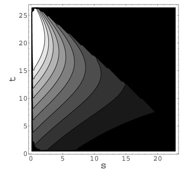
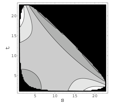
Figure 2: Dalitz plots for the non-resonant $B^{-}\to K^{-}\pi^{-}\pi^{+}$ (left) and $B^{-}\to K^{-}K^{-}K^{+}$ (right) decay modes.

3 PARTIAL WIDTH ASYMMETRY

For the resonances in the s-channel, the partial decay width $\Gamma_{p}$ for $B^{-}\to M{\bar{M}}K^{-}$, $M=\pi^{+}$, $K^{+}$, which contains both the non-resonant and resonant contributions, is obtained by integrating the amplitude from $s_{min}=(m_{R}-2\Gamma_{R})^{2}$ to $s_{max}=(m_{R}+2\Gamma_{R})^{2}$:

$$\Gamma_{p}=\frac{1}{(2\pi)^{3}}\frac{1}{32m_{B}^{3}}\int_{s_{min}}^{s_{max}}ds\int_{t_{min}(s)}^{t_{max}(s)}dt\leavevmode\nobreak\ |{\cal M}_{nr}+{\cal M}_{r}|^{2}.$$ (21)

Similarly, the partial decay width $\Gamma_{\bar{p}}$ for $B^{+}\to M{\bar{M}}K^{+}$, $M=\pi^{+}$, $K^{+}$ is defined in a same way. The CP violating asymmetry is then:

$$A_{p}=\frac{|\Gamma_{p}-\Gamma_{\bar{p}}|}{|\Gamma_{p}+\Gamma_{\bar{p}}|}.$$ (22)

It is important to notice that at the phase space region where the invariant mass of $M^{+}M^{-}$ approaches the mass of the ${\cal R}$ resonant state, $M^{+}M^{-}$ can re-scatter trough that resonance as it is visualized in Fig. 3 (left figure). If $Br({\cal R}\to M^{+}M^{-}$) is large, this can lead to a significant absorptive amplitude and it contributes to the partial decay width asymmetry. As mentioned in Introduction and explained in Appendix, such contribution is exactly canceled by the absorptive part of a resonant decay, where the resonance re-scatters trough the intermediate states equal to final states (Fig. 3 (right figure)). This implies that one has include the factor (1 - Br(${\cal R}\to M^{+}M^{-}$)) in the equation for the partial decay asymmetry.

In the calculation of the $\Gamma_{p}-\Gamma_{\bar{p}}$, by taking $V_{ub}=|V_{ub}|e^{i\gamma}$ $\simeq A\lambda^{3}(\bar{\rho}-i\bar{\eta})$, we derive:

$$\Gamma_{p}-\Gamma_{\bar{p}}=\sin\gamma\frac{4m_{R}\Gamma_{R}(1-Br({\cal R}\to M^{+}M^{-}))}{(2\pi)^{3}32m_{B}^{3}}$$

$$\times\int_{s_{min}}^{s_{max}}ds\int_{t_{min}(s)}^{t_{max}(s)}dt\leavevmode\nobreak\ \frac{G}{{\sqrt{2}}}|V_{ub}||V_{us}^{*}|a_{1}<K\pi\pi|O_{1}|B>_{\rm nr}$$

$$\times|{\cal M}(B^{-}\to RK^{-})|\frac{1}{(s-m_{R}^{2})^{2}+(m_{R}\Gamma_{R})^{2}}|{\cal M}(R\to\pi^{-}\pi^{+})|,$$

(23)

while the $\Gamma_{p}+\Gamma_{\bar{p}}$ is given by:

$$\Gamma_{p}+\Gamma_{\bar{p}}=2\frac{1}{(2\pi)^{3}32m_{B}^{3}}\int_{s_{min}}^{s_{max}}ds\int_{t_{min}(s)}^{t_{max}(s)}dt\leavevmode\nobreak\$$

$$\times\{|{\cal M}_{\rm nr}|^{2}+|{\cal M}(B^{-}\to RK^{-})\frac{1}{s-m_{R}^{2}+im_{R}\Gamma_{R}}{\cal M}(R\to\pi^{-}\pi^{+})|^{2}\}.$$

(24)

The $B^{-}\to{\cal R}K^{-}\to K^{-}M^{+}M^{-}$ amplitudes are obtained from the experimental data [29] and the measured branching ratios for $B^{-}\to{\cal R}K^{-}$ and $R\to M^{+}M^{-}$ are given in Table 1.

R	$B^{-}\to{\cal R}K^{-}$	${\cal R}\to\pi^{+}\pi^{-}$	${\cal R}\to K^{+}K^{-}$
$\phi$	$(7.9\pm 2.0)\times 10^{-6}$		$(49.2\pm 0.7)$%
$J/\psi$	$(1.01\pm 0.05)\times 10^{-3}$	$(1.47\pm 0.23)\times 10^{-4}$	$(2.37\pm 0.0.31)\times 10^{-4}$
$\chi_{c0}$	$(6.5\pm 1.1)\times 10^{-4}$	$(5.0\pm 0.7)\times 10^{-3}$	$(5.9\pm 0.9)\times 10^{-3}$
$\chi_{c1}$	$(6.0\pm 2.4)\times 10^{-4}$	$<2.1\times 10^{-3}$	$<2.1\times 10^{-3}$
$\psi(2S)$	$(6.6\pm 0.6)\times 10^{-4}$	$(8\pm 5)\times 10^{-5}$	$(1.0\pm 0.7)\times 10^{-4}$

Table 1: The decay $B^{-}\to{\cal R}K^{-}$ width and the branching ratios for ${\cal R}\to M^{+}M^{-}$.

For the scalar resonance exchange ($\chi_{0}$ in our case) in the $B^{-}\to SK^{-}\to M^{+}M^{-}K^{-}$ decay, we have:

$${\cal M}(B^{-}\to SP_{1}(q_{1})\to P_{1}(q_{1})P_{2}(q_{2})P_{3}(q_{3}))=$$

$${\cal M}(B^{-}\to SP_{1}(q_{1}))\frac{1}{m_{23}^{2}-m_{S}^{2}+i\Gamma_{S}m_{S}}{\cal M}(S\to P_{2}(q_{2})P_{3}(q_{3}))\,,$$ (25)

where $m^{2}_{23}=(q_{2}+q_{3})^{2}$ while $m_{S}$ and $\Gamma_{S}$ are the mass and the decay width of the scalar resonance respectively. We find ${\cal M}(B^{-}\to\chi_{c0}K^{-})=3.34\times 10^{-7}$ GeV, ${\cal M}(\chi_{co}\to\pi^{+}\pi^{-})=0.118$ GeV and ${\cal M}(\chi_{co}\to K^{+}K^{-})=0.132$ GeV.

The amplitude for the $B^{-}$ decay into light vector and pseudoscalar resonance and the amplitude for the vector meson decay into two pseudoscalar states are given by:

$${\cal M}(B^{-}\to V(\varepsilon)P_{1}(q_{1}))=Kq_{1}\cdot\varepsilon^{*}\,,\qquad{\cal M}(V\to P_{2}(q_{2})P_{3}(q_{3}))=\frac{g_{VP_{2}P_{3}}}{\sqrt{2}}(q_{2}-q_{3})\cdot\varepsilon.$$ (26)

The amplitude for the three-body resonant decay for this case is:

$${\cal M}(B^{-}\to V(\varepsilon)P_{1}(q_{1})\to P_{1}(q_{1})P_{2}(q_{2})P_{3}(q_{3}))=$$

$$\frac{Kg_{VP_{2}P_{3}}}{\sqrt{2}}\frac{-q_{1}\cdot(q_{2}-q_{3})+(q_{1}\cdot(q_{2}+q_{3})(m^{2}_{2}-m^{2}_{3}))/m_{V}^{2}}{m^{2}_{23}-m_{V}^{2}+i\Gamma_{V}m_{V}}\,,$$ (27)

where $m^{2}_{23}=(q_{2}+q_{3})^{2}$, while $m_{1}$, $m_{2}$, $m_{3}$ and $m_{V}$ are the masses of particles $P_{1}$, $P_{2}$, $P_{3}$ and $V$ respectively and $\Gamma_{V}$ is the width of the vector resonance. Using above formulas, we find the expression for the resonance exchange in the $s-$channel:

$${\cal M}(B^{-}\to VK^{-}\to K^{-}M^{+}M^{-})=\frac{K_{V}g_{VMM}}{2\sqrt{2}}\frac{m_{B}^{2}+2m_{M}^{2}+m_{K}^{2}-2t-s}{s-m_{V}^{2}+i\Gamma_{V}m_{V}}\,,$$ (28)

where $M$ stands for $K$ or $\pi$. In the case of the $K^{-}K^{+}K^{\pm}$ mode the contributions coming from the $s$ and $t$ channels are completely symmetric. Values of $K_{V}$ and $g_{VP_{1}P_{2}}$ are given in Table 2.

$V$	$K_{V}$	$g_{V\pi\pi}$	$g_{VKK}(g_{VK\pi})$
$\phi$	$2.26\times 10^{-9}$		6.34
$J/\psi$	$1.41\times 10^{-7}$	$2.76\times 10^{-4}$	$4.37\times 10^{-3}$
$\psi(2S)$	$2.04\times 10^{-7}$	$1.41\times 10^{-3}$	0.166
$\chi_{c1}$	$1.68\times 10^{-7}$	$<0.0126$	$<0.0134$

Table 2: The parameters used in our numerical calculations.

	$\bar{\rho}=0.118$	$\bar{\rho}=0.118$	$\bar{\rho}=0.273$	$\bar{\rho}=0.273$	$\bar{\rho}=0.222$
	$\bar{\eta}=0.305$	$\bar{\eta}=0.393$	$\bar{\eta}=0.305$	$\bar{\eta}=0.393$	$\bar{\eta}=0.339$
$A_{p}$($\psi(2S)$)	10.2%	13.0%	10.3%	13.1%	11.3%
$A_{p}$($J/\psi$)	0.8%	1.1%	0.8%	1.1%	0.9%
$A_{p}$($\chi_{c1}$)	3.5%	4.5%	3.5%	4.5%	3.9%
$A_{p}$($\chi_{c0}$)	17.3%	21.8%	17.6%	22.1%	19.3%

Table 3: The partial width asymmetry for $B^{-}\to K^{-}\pi^{+}\pi^{-}$, calculated with $g=0.56$ and given $\bar{\rho}$ and $\bar{\eta}$. $A_{p}$($\chi_{c1}$) is obtained by taking the upper bound for $g_{VMM}$.

	$\bar{\rho}=0.118$	$\bar{\rho}=0.118$	$\bar{\rho}=0.273$	$\bar{\rho}=0.273$	$\bar{\rho}=0.222$
	$\bar{\eta}=0.305$	$\bar{\eta}=0.393$	$\bar{\eta}=0.305$	$\bar{\eta}=0.393$	$\bar{\eta}=0.339$
$A_{p}$($\psi(2S)$)	13.5%	17.3%	13.7%	17.3%	15.1%
$A_{p}$($J/\psi$)	1.2%	1.6%	1.2%	1.6%	1.4%
$A_{p}$($\chi_{c1}$)	5.0%	6.4%	5.0%	6.5%	5.6%
$A_{p}$($\chi_{c0}$)	12.8%	16.1%	12.9%	16.3%	14.2%

Table 4: The partial width asymmetry for $B^{-}\to K^{-}\pi^{+}\pi^{-}$, calculated with $g=0.27$ and given $\bar{\rho}$ and $\bar{\eta}$. $A_{p}$($\chi_{c1}$) is obtained by taking the upper bound for $g_{VMM}$.

	$\bar{\rho}=0.118$	$\bar{\rho}=0.118$	$\bar{\rho}=0.273$	$\bar{\rho}=0.273$	$\bar{\rho}=0.222$
	$\bar{\eta}=0.305$	$\bar{\eta}=0.393$	$\bar{\eta}=0.305$	$\bar{\eta}=0.393$	$\bar{\eta}=0.339$
$A_{p}$($\phi$)	0.3%	0.3%	0.3%	0.3%	0.3%
$A_{p}$($\psi(2S)$)	3.1%	3.8%	3.0%	3.7%	3.3%
$A_{p}$($J/\psi$)	0.03%	0.04%	0.03%	0.04%	0.03%
$A_{p}$($\chi_{c1}$)	0.5%	0.7%	0.5%	0.3%	0.6%
$A_{p}$($\chi_{c0}$)	28.8%	35%	27.6%	33.8%	30.6%

Table 5: The partial width asymmetry for $B^{-}\to K^{-}K^{+}K^{-}$, calculated with $g=0.56$ and given $\bar{\rho}$ and $\bar{\eta}$. $A_{p}$($\chi_{c1}$) is obtained by taking the upper bound for $g_{VMM}$.

	$\bar{\rho}=0.118$	$\bar{\rho}=0.118$	$\bar{\rho}=0.273$	$\bar{\rho}=0.273$	$\bar{\rho}=0.222$
	$\bar{\eta}=0.305$	$\bar{\eta}=0.393$	$\bar{\eta}=0.305$	$\bar{\eta}=0.393$	$\bar{\rho}=0.339$
$A_{p}$($\phi$)	0.3%	0.3%	0.3%	0.3%	0.3%
$A_{p}$($\psi(2S)$)	8.1%	10.1%	7.9%	9.8%	8.8%
$A_{p}$($J/\psi$)	0.55%	0.71%	0.55%	0.71%	0.61%
$A_{p}$($\chi_{c1}$)	3.0%	3.8%	3.0%	3.8%	3.3%
$A_{p}$($\chi_{c0}$)	23.1%	28.7%	22.5%	28.0%	25%

Table 6: The partial width asymmetry for $B^{-}\to K^{-}K^{+}K^{-}$, calculated with $g=0.27$ and given $\bar{\rho}$ and $\bar{\eta}$. $A_{p}$($\chi_{c1}$) is obtained by taking the upper bound for $g_{VMM}$.

The results for the asymmetries are presented in Tables 3-6. Tables 3 and 5 contain the asymmetries for $g=0.56$. The off-shell mass effects might reduce this coupling as mentioned in [5], and therefore we present the partial width asymmetries for $g=0.27$ (Tables 4 and 6). We calculate asymmetries for the ranges $\bar{\rho}=0.118-0.273$ (the average value 0.222) and $\bar{\eta}=0.305-0.393$ (the average value 0.339) as in [22]. The subtraction of $Br({\cal R}\to M^{+}M^{-})$ in Eq. (23) makes a sizable effect in the case of the $B^{-}\to K^{-}\phi\to M^{+}M^{-}K^{-}$ asymmetry, but it is negligible in the case of partial width asymmetry in the neighborhood of charmonium resonances. Then we can draw the following conclusions: In the case of $B^{-}\to K^{-}\pi^{+}\pi^{-}$, all partial width asymmetries are not very large. The largest asymmetry was found in the case of $\chi_{c0}$ resonance and then in the case of $\psi(2S)$. The partial width asymmetry $A_{p}(\chi_{c1})$ is calculated by taking the upper bounds for $\chi_{c1}M^{+}M^{-}$ coupling. All these asymmetries are rather stable on the variations of $g$. In the case of $B^{-}\to K^{-}K^{+}K^{-}$ the situation is different. Calculated partial width asymmetries except the $A_{p}(\chi_{c0})$ are smaller than in the case of $B^{-}\to K^{-}\pi^{+}\pi^{-}$. They depend more on the variations of the $g$ coupling. The only relatively sizable partial width asymmetry in addition to $A_{p}(\chi_{c0})$ is $A_{p}(\psi(2s))$.

We have also estimated the partial width asymmetry for the $B^{-}\to\chi_{c2}K^{-}$ channel, by assuming the $B_{\chi_{c2}K}$ coupling to be of the same size as for the vector (scalar) mesons and we found it negligible.

4 SUMMARY

In this paper we have investigated the partial width asymmetry for the $B^{-}\to M^{+}M^{-}K^{-}$, $M=\pi,K$ decays which results from the interference of non-resonant and resonant amplitudes.

First, we have calculated the non-resonant branching ratios and found that the model we use gives the decay rates in the reasonable agreement with the Belle collaboration results [3]. Comparing the Dalitz plots for the non-resonant decay modes obtained from our model with the experimental data [3], we find that our model reproduces the data quite well. The inclusion of the $B^{*}_{0}$ scalar meson is rather insignificant, contributing only by few percents to the rate.

We then consider the partial width asymmetries for a few resonant decay modes for which the amplitude does not contain the weak phase $\gamma$. In the case of $B^{-}\to\pi^{+}\pi^{-}K^{-}$ the largest partial width asymmetry arises from the interference of the non-resonant amplitude with the resonant amplitude coming from the $\chi_{c0}$ and $\psi(2S)$ states. In the case of $B^{-}\to K^{-}K^{+}K^{-}$ the largest partial width asymmetry comes from the $\chi_{c0}$ scalar resonance, while and is about $\leavevmode\nobreak\ 10\%$ in the case of $\psi(2S)$ state.

ACKNOWLEDGMENTS

We thank our colleagues B. Golob and P. Križan for stimulating discussions on experimental aspects of this investigation and D. Bećirević for very useful comments. The research of S. F. and A. P. was supported in part by the Ministry of Education, Science and Sport of the Republic of Slovenia.

APPENDIX

Figure 3: Diagrams presenting the non-resonant (left) and the resonant (right) contributions to dispersive part of the amplitude in the phase space region of the $P_{2}$ and $P_{3}$ invariant mass close to the ${\cal R}$ mass. Blob in the left diagram presents the non-resonant weak decay mode (see Fig. 1).

Following the approach of [15], the total amplitude contributing to the partial decay width $\Gamma_{p}$ can be written as a sum of the resonant and nonresonant contributions as defined in Eq. (21) in the following form:

$${\cal M}={\cal M}_{nr}+{\cal M}_{r}=Te^{-i\gamma}+P+R\,,$$ (29)

where $T$ is the nonresonant tree contribution, $P$ the nonresonant penguin contribution and $R$ the resonant contribution to the amplitude. The partial width asymmetry defined in Eq. (22) is proportional to:

$$A_{p}\propto\sin\gamma\;\Im(T(P^{*}+R^{*}))\,,$$ (30)

where $\Im(A)$ stands for the imaginary part of $A$ (similarly $\Re(A)$ stands for the real part of $A$). If we neglect the small imaginary part of the penguin Wilson coefficients, $T$ and $P$ will have the same strong phase. This implies that the only contribution to the partial decay asymmetry will come from the interference of the tree nonresonant and the resonant amplitude. One can write:

$$A_{p}\propto\Im(T)\Re(R)-\Im(R)\Re(T)\,.$$ (31)

The imaginary part of $T$ is given by the absorptive part of the left diagram on the Fig. 3. Using Cutkosky’s rules, its contribution can be written as:

$$\Im(T)\Re(R)=\frac{(2\pi)^{4}}{2}\int\Re(T)\Re(R)\Re(S)d\Phi\,,$$ (32)

where the integration is taken over the $P_{2}P_{3}$ phase space. Here $S$ denotes the strong re-scattering amplitude of $P_{2}P_{3}$ trough the resonance ${\cal R}$ visualized in Fig. 4. Similarly, the imaginary part of $R$ is given by the absorptive part of the right diagram on the Fig. 3, where now the sum of all possible intermediate states into which ${\cal R}$ decays should be taken into account. One can separate this contribution into the part with $P_{2}$ and $P_{3}$ as an intermediate state ($\Im(R)_{P_{2,3}}$) and the part with all other intermediate states ($\Im(R)^{\prime}$). Again with the use of Cutkosky’s rules, one obtains:

$$\Im(R_{P_{2,3}})\Re({T}=\frac{(2\pi)^{4}}{2}\int\Re(T)\Re(R)\Re(S)d\Phi\,.$$ (33)

The right hand sides of (33) and (32) are equal and therefore this two contributions to (31) cancel among themselves and we have:

$$A_{p}\sim\Im(R)^{\prime}\Re(T)\sim\Gamma_{R}(1-Br({\cal R}\to P_{2}P_{3})\Re(T)\,.$$ (34)

This cancellation is obviously a result of the unitarity and it maintains the equality of the total decay widths for the meson and the anti-meson as required by CPT theorem [30]. That was already noticed by [9] and [15], where the more general proof is presented.

Figure 4: Re-scattering of the $P_{2}$ and $P_{3}$ states trough the resonance ${\cal R}$.

References

[1] J. R. Fry, talk given at Lepton Photon Conference,
Fermilab, 2003.
[2] BELLE Collaboration, K. Abe et al., Phys. Rev. Lett. 88, 031802 (2002).
[3] BELLE Collaboration, K. Abe et al., BELLE-CONF-0338.
[4] B. Aubert et al., Phys. Rev. Lett. 91, 051801 (2003).
[5] S. Fajfer, R. J. Oakes and T. N. Pham,
Phys. Lett B 539, 67 (2002).
[6] B. Bajc, S. Fajfer, R. J. Oakes, T. N. Pham
and S. Prelovšek, Phys. Lett. B 447, 313 (1999).
[7] N. G. Deshpande, G. Eilam, X. G. He, and J.
Trampetić,
Phys. Rev. D 52, 5354 (1995).
[8] H. Y. Cheng and K. C. Yang, Phys. Rev. D 66, 054015
(2002).
[9] G. Eilam, M. Gronau and R. R. Mendel, Phys. Rev. Lett.
74, 4984 (1995).
[10] S. Fajfer, R. J. Oakes, T. N. Pham, Phys. Rev.
D 60, 054029 (1999).
[11] I. Bediaga, R. E. Blanco, C. Göbel, and R. Mendez-Galain,
Phys. Rev. Lett. 81, 4067 (1998).
[12] R. E. Blanco, C. Göbel, and R. Mendez-Galain,
Phys. Rev. Lett. 86, 2720 (2001).
[13] R. Enomoto, Y. Okada, and Y. Shimizu,
Phys. Lett. B 433, 109 (1998).
[14] M. Hazumi, Phys. Lett. B 583, 285 (2004).
[15] H. Simma, G. Eliam, D. Wyler, Nucl. Phys. B 352,
367 (1991).
[16] A. Ali, G. Kramer, C. D. Lü, Phys. Rev. D 59,
014005 (1999).
[17] A. Ali, G. Kramer, C. D. Lü, Phys. Rev. D 58,
094009 (1999).
[18] A. Ali, C. Greub, Phys. Rev. D 57,
2996 (1998).
[19] N. G. Deshpande, X. G. He, Phys. Lett. B 336,
471 (1994); N. G. Deshpande, X. G. He, W. S. Hou, S. Pakvasa,
Phys. Rev. Lett. 82, 2240 (1999).
[20] C. Isola, T. N. Pham, Phys. Rev. D 62, 094002
(2000).
[21] T. E. Browder, A. Datta, X. G. He, S. Pakvasa,
Phys. Rev. D 57, 6829 (1998).
[22] data taken from www.ckmfitter.in2p3.fr; A. Hocker et al.,
Eur. Phys. J. C 21, 225 (2001).
[23] B. Bajc, S. Fajfer, R. J. Oakes, T. N. Pham,
Phys. Rev. D 58, 054009 (1998).
[24] B. Bajc, S. Fajfer, R. J. Oakes, S. Prelovsek,
Phys. Rev. D 56, 7207, (1997).
[25] S. Fajfer, R. J. Oakes, T. N. Pham, Phys. Rev. D
60, 054029 (1999).
[26] R. Casalbuoni et al., Phys. Rep. 281, 145 (1997).
[27] P. Colangelo, F. De Fazio, Phys. Lett. B 570, 180
(2003).
[28] CLEO collaboratio, T. E. Coan et al., hep-ex/0102007.
[29] Particle Data Group, K. Hagiwara at al.,
Phys. Rev D 66, 010001 (2002).
[30] J-M. Gerard, W-s. Hou, Phys. Rev. Lett. B 62, 855
(1989); L. Wolfenstein, Phys. Rev. D 43, 151 (1991); D. Atwood,
A. Soni, Phys. Rev. D 58, 036005 (1998).