Pion form factor in QCD: From nonlocal condensates to NLO analytic perturbation theory

Abstract

We present an investigation of the pion’s electromagnetic form factor $F_{\pi}(Q^{2})$ in the spacelike region utilizing two new ingredients: (i) a double-humped, endpoint-suppressed pion distribution amplitude derived before via QCD sum rules with nonlocal condensates—found to comply at the $1\sigma$ level with the CLEO data on the $\pi\gamma$ transition—and (ii) analytic perturbation theory at the level of parton amplitudes for hadronic reactions. The computation of $F_{\pi}(Q^{2})$ within this approach is performed at NLO of QCD perturbation theory (standard and analytic), including the evolution of the pion distribution amplitude at the same order. We consider the NLO corrections to the form factor in the $\overline{\text{MS}\vphantom{{}^{1}}}$ scheme with various renormalization scale settings and also in the $\alpha_{V}$-scheme. We find that using standard perturbation theory, the size of the NLO corrections is quite sensitive to the adopted renormalization scheme and scale setting. The main results of our analysis are the following: (i) Replacing the QCD coupling and its powers by their analytic images, both dependencies are diminished and the predictions for the pion form factor are quasi scheme and scale-setting independent. (ii) The magnitude of the factorized pion form factor, calculated with the aforementioned pion distribution amplitude, is only slightly larger than the result obtained with the asymptotic one in all considered schemes. (iii) Including the soft pion form factor via local duality and ensuring the Ward identity at $Q^{2}=0$, we present predictions that are in remarkably good agreement with the existing experimental data both in trend and magnitude.

I Introduction

It is the purpose of this paper to review and discuss questions relating to the calculation of the electromagnetic pion form factor with an improved pion distribution amplitude (DA), derived from QCD sum rules with nonlocal condensates Bakulev et al. (2001), and to use QCD Analytic Perturbation Theory (APT) Solovtsov and Shirkov (1999); Shirkov (2001a, 2000, b, c) beyond the leading order (LO). Before going into the details of this framework, let us expose, in general terms, what these two ingredients mean for the analysis and also make some introductory remarks.

Hadronic form factors are typical examples of hard-scattering processes within QCD Chernyak and Zhitnitsky (1977); Chernyak et al. (1977); Efremov and Radyushkin (1980a, b); Lepage and Brodsky (1979, 1980) and clearly the first level of knowledge necessary to understand the structure of intact hadrons in terms of quarks and gluons. Such processes have been much explored both because of their physical relevance, as being accessible to experiments, and because they allow to assess nonperturbative features of QCD (for reviews, see, for instance, Chernyak and Zhitnitsky (1984); Brodsky and Lepage (1989); Mueller (1997); Stefanis (1999); Goeke et al. (2001)). In the following, the discussion is centered around the pion’s electromagnetic form factor. At a more theoretical level, “hard” means that at least some part of the process amplitude, recast in terms of quarks collinear to hadrons (in an appropriate Lorentz frame), should become amenable to perturbation theory via factorization theorems on account of the hard-momentum scale of the process, say, $Q^{2}$, that should suppress factorized infrared (IR) subprocesses, thus ensuring short-distance dominance. Under these circumstances one can safely evaluate logarithmic scaling violations by means of perturbative QCD (pQCD) and the renormalization-group equation. When no hard momenta flow on the side of the initial (incoming) or the final (outgoing) hadron, factorization fails and a renormalization-group analysis cannot be made, so that in order to calculate the non-factorizable part of the pion form factor, one has to resort to phenomenological models (prime examples of which are Isgur and Llewellyn Smith (1984); Jacob and Kisslinger (1986); Isgur and Llewellyn Smith (1989); Jakob and Kroll (1993)), or employ theoretical concepts like the (local) quark-hadron duality Shifman et al. (1979) and their descendants Nesterenko and Radyushkin (1982); Radyushkin (1995); Bakulev et al. (2000).

Despite dedicated efforts in the last two decades, exclusive processes have failed to deliver a complete quantitative understanding within QCD for a variety of reasons, among others:

• Limited knowledge of higher-order perturbative and power-law behaved (e.g., higher-twist) corrections to the amplitudes.

• Presence of singularities (of endpoint, mass, soft, collinear, or pinch origin) that may spoil factorization in some kinematic regions.

• Insignificant knowledge of hadron distribution amplitudes owing to the lack of a reliable non-perturbative approach.

• Non-factorizing contributions that are not calculable within pQCD and hence introduce a strong model dependence.

While it may still be not possible to clarify all these theoretical issues conclusively, we believe that significant progress has quite recently been achieved in understanding the pion structure both from the theoretical side—perturbatively Melić et al. (1999, 2002); Stefanis et al. (1999, 2000); Melić et al. (2003) and nonperturbatively Bakulev et al. (2001); Khodjamirian (1999); Braun et al. (2000); Bijnens and Khodjamirian (2002); Bakulev et al. (2003a)—as well as from the experimental side Gronberg et al. (1998); Volmer et al. (2001); Blok et al. (2002) and associated data-processing techniques Schmedding and Yakovlev (2000); Bakulev et al. (2003b, 2004), a progress that could bring to a cleaner comparison between data and various theoretical QCD predictions Radyushkin and Ruskov (1996); Jakob et al. (1996); Kroll and Raulfs (1996); Musatov and Radyushkin (1997); Brodsky et al. (1998); Khodjamirian (1999); Diehl et al. (2001); Bakulev et al. (2003b, 2004); Bakulev et al. (2003c); Agaev (2004); Huang et al. (2004). Moreover, a program to compute the electromagnetic and transition form factors of mesons on the lattice has been launched by two collaborations, Bonnet et al. (2003a, b) and Nemoto (2003), that may provide valuable insights when it is completed. This situation prompts an in-depth review and update of these issues, in an effort to consolidate previous calculations of the pion’s electromagnetic form factor and narrow down theoretical uncertainties.

We will focus our present discussion on two main issues:

1. How QCD perturbation theory can be safely used to make predictions in the low-momentum regime where conventional power series expansions in the QCD coupling break down and nonperturbative effects dominate. Such an extension is based on recent works on “analytization” of the running strong coupling $\alpha_{\rm s}(Q^{2})$ Dokshitzer et al. (1996); Grunberg (1997); Shirkov and Solovtsov (1997); Shirkov (1999); Gardi et al. (1998); Solovtsov and Shirkov (1999); Shirkov (2001a, c) (see also Nesterenko (2003) for a slightly different approach) and their generalization to the partonic level of hadron amplitudes, like the electromagnetic and the pion-photon transition form factor, or the Drell–Yan process, beyond the level of a single scheme scale Stefanis et al. (1999, 2000); Karanikas and Stefanis (2001); Stefanis (2003). In contradiction to the usual assumption of singular growth of $\alpha_{\rm s}(Q^{2})$ in the IR domain, the QCD coupling in this scheme has an IR-fixed point, with the unphysical Landau pole being completely absent. In conventional perturbative approaches, a choice of the renormalization scale in the region of a few $\Lambda_{\rm QCD}$, as required, for instance, by the Brodsky–Lepage–Mackenzie (BLM) scale-fixing procedure Brodsky et al. (1983a), would induce singularities thus prohibiting the perturbative calculation of hadronic observables. Using APT, these singularities are avoided by construction, i.e., without introducing ad hoc IR regulators, e.g., an effective gluon mass Brodsky and Lepage (1989); Ji and Amiri (1990), and therefore the validity of the perturbative expansion (in mass-independent renormalization schemes) is not jeopardized by IR-renormalon power-law ambiguities. In addition, APT provides a better stability against higher-loop corrections and a weaker renormalization-scheme dependence than standard QCD perturbative expansion—see Stefanis et al. (2000) and Sec. VIId.

2. How to improve the nonperturbative input by employing a pion DA which incorporates the nonperturbative features of the QCD vacuum in terms of a nonlocal quark condensate Mikhailov and Radyushkin (1986a, 1989, 1992); Bakulev and Radyushkin (1991); Bakulev and Mikhailov (1995). This accounts for the possibility that vacuum quarks can flow with a nonzero average virtuality $\lambda_{q}^{2}$, in an attempt to connect dynamic properties of the pion, like its electromagnetic form factor, directly with the QCD vacuum structure (we refer to Bakulev et al. (2003a) for further details). Within this scheme, the pion DA (termed BMS Bakulev et al. (2001) in the following) turns out to be double-humped with strongly suppressed endpoints ($x=0,1$), the latter feature being related to the nonlocality parameter $\lambda_{q}^{2}$. It has been advocated, for example, in Stefanis et al. (1999, 2000) (see also Stefanis (1995, 1999)), that a suppression of the endpoint region (which is essentially nonperturbative) as strong as possible is a prerequisite for the self-consistent application of QCD perturbation theory within a factorization scheme.

In a recent series of papers Bakulev et al. (2001, 2003b, 2004), two of us together with S. V. Mikhailov have conducted an analysis of the CLEO data Gronberg et al. (1998) on the pion-photon transition using attributes from QCD light-cone sum rules Khodjamirian (1999); Schmedding and Yakovlev (2000), NLO Efremov–Radyushkin–Brodsky–Lepage (ERBL) Efremov and Radyushkin (1980a, b); Lepage and Brodsky (1979, 1980) evolution Müller (1994, 1995), and detailed estimates of uncertainties owing to higher-twist contributions and NNLO perturbative corrections Melić et al. (2003). These works confirmed the gross features of the previous Schmedding–Yakovlev (SY) analysis Schmedding and Yakovlev (2000); notably, both the Chernyak–Zhitnitsky (CZ) Chernyak and Zhitnitsky (1984) pion DA as well as the asymptotic one are incompatible with the CLEO data Gronberg et al. (1998) at the $4\sigma$- and $3\sigma$-level, respectively, whereas the aforementioned BMS pion DA, which incorporates the vacuum nonlocality, is within the $1\sigma$ error ellipse. Moreover, this approach revealed the possibility of using the CLEO experimental data to estimate the value of the QCD vacuum correlation length $\lambda_{q}^{-1}$. Indeed, it turns out that the extracted value $\lambda_{q}^{2}\simeq 0.4$ GeV² is consistent with those obtained before using QCD sum rules Belyaev and Ioffe (1983); Ovchinnikov and Pivovarov (1988); Kataev et al. (2003) and also with numerical simulations on the lattice D’Elia et al. (1999); Bakulev and Mikhailov (2002). In addition, it was shown Bakulev et al. (2004) that the value of the inverse moment $\langle x^{-1}\rangle_{\pi}(\mu^{2})=\int^{1}_{0}\varphi_{\pi}(x;\mu^{2}){x}^{-1}dx$ of the pion DA, calculated by means of an independent QCD sum rule, is compatible with that extracted from the CLEO data. These findings give us confidence to use the BMS pion DA (including also the range of its intrinsic theoretical uncertainties) in order to derive predictions for the electromagnetic pion form factor within the factorization scheme of QCD at NLO, presenting also results which include the non-factorizing soft contribution Nesterenko and Radyushkin (1982); Bakulev et al. (2000) to compare with available experimental data.

The structure of the paper is as follows. In Sec. II we shall recall the QCD factorization of the pion’s electromagnetic form factor. Sec. III deals with the basics of the pion distribution amplitude and its derivation from QCD sum rules with nonlocal condensates. The perturbative results for the pion form factor at NLO order, on the basis of the results given in Melić et al. (1999), are summarized in Sec. IV, whereas issues related to the setting of the renormalization scheme and scale are discussed in Sec. V. The important topic of the non-power series expansion of the pion form factor in the context of Analytic Perturbation Theory is considered in Sec. VI. Our numerical analysis and the comparison of our results with available experimental data is presented in Sec. VII. Finally, in Sec. VIII we give a summary of the results and draw our conclusions. Important technical details of the analysis are supplied in five appendixes.

II QCD factorization applied to the pion form factor

The outstanding virtue of factorization is that a hadronic process can be dissected in such a way as to isolate a partonic part accessible to pQCD. Provided that the partonic subprocesses are free of IR-singularities, then at large momentum transfer $F_{\pi}(Q^{2})/f_{\pi}^{2}\sim 1/Q^{2}$, modulo logarithmic corrections due to renormalization. Hence, the amplitude for the electromagnetic pion form factor is short-distance dominated and can be expressed in terms of its constituent quarks collinear to the pion with the errors of this replacement being suppressed by powers of $1/Q$. Even more, one can rigorously dissect the QCD amplitude into a coefficient function, that contains the hard quark-gluon interactions, and two matrix elements corresponding to the initial and final pion states of the leading twist operator with the quantum numbers of the pion according to the Operator Product Expansion (OPE). In this way, one establishes that the coefficient function will scale asymptotically according to its dimensionality modulo anomalous dimensions controlled by the renormalization group equation.

The pion’s electromagnetic form factor is defined by the matrix element

$$\langle{\pi^{+}(P^{\prime})|J_{\mu}(0)|\pi^{+}(P)}\rangle={\left(P+P^{\prime}\right)}_{\mu}F_{\pi}(Q^{2})\,,$$ (1)

where $J_{\mu}$ is the electromagnetic current expressed in terms of quark fields, $(P^{\prime}-P)^{2}=q^{2}\equiv-Q^{2}$ is the photon virtuality, i.e., the large momentum transfer injected into the pion, and $F_{\pi}$ is normalized to $F_{\pi}(0)=1$. Based on the above considerations, the pion form factor can be generically written in the form Efremov and Radyushkin (1980a, b); Lepage and Brodsky (1979, 1980)

$$F_{\pi}(Q^{2})=F_{\pi}^{\text{Fact}}(Q^{2})+F_{\pi}^{\text{non-Fact}}(Q^{2})\,,$$ (2)

where $F_{\pi}^{\text{Fact}}(Q^{2})$ is the factorized part within pQCD and $F_{\pi}^{\text{non-Fact}}(Q^{2})$ is the non-factorizable part—usually being referred to as the “soft contribution” Nesterenko and Radyushkin (1982)—that contains subleading power-behaved (e.g., twist-4 and higher-twist) contributions originating from nonperturbative effects. It is important to understand that Eq. (2) becomes increasingly unreliable as $Q^{2}\to 0$, owing to the breakdown of perturbation theory at such low momentum scales. Hence, we expect the real form factor to be different from the RHS of this equation at low $Q^{2}$. We shall show in Sec. VII.4 how to remedy this problem. The leading-twist factorizable contribution can be expressed as a convolution in the form

$$F_{\pi}^{\text{Fact}}(Q^{2};\mu_{\text{R}}^{2})=\Phi_{\pi}^{*}(x,\mu_{\text{F}}^{2})\mathop{\otimes}\limits_{x}T_{\text{H}}(x,y,Q^{2};\mu_{\text{F}}^{2},\mu_{\text{R}}^{2})\mathop{\otimes}\limits_{y}\Phi_{\pi}(y,\mu_{\text{F}}^{2})\,,$$ (3)

where $\otimes$ denotes the usual convolution symbol ($A(z)\mathop{\otimes}\limits_{z}B(z)\equiv\int_{0}^{1}dzA(z)B(z)$) over the longitudinal momentum fraction variable $x$ ($y$) and $\mu_{\text{F}}$ represents the factorization scale at which the separation between the long- (small transverse momentum) and short-distance (large transverse momentum) dynamics takes place, with $\mu_{\text{R}}$ standing for the renormalization (coupling constant) scale. A graphic illustration of the factorized pion form factor in terms of Feynman diagrams is given in Fig. 1.

Figure 1: Illustration of the structure of the factorized pion form factor within pQCD at NLO of the hard scattering amplitude and the evolution effect of the pion DA. Hard gluons are indicated by broken lines, whereas the external off-shell photon is denoted by a cross.

Here, $T_{\text{H}}(x,y,Q^{2};\mu_{\text{F}}^{2},\mu_{\text{R}}^{2})$ is the hard-scattering amplitude, describing short-distance interactions at the parton level, i.e., it is the amplitude for a collinear valence quark-antiquark pair with total momentum $P$ struck by a virtual photon with momentum $q$ to end up again in a configuration of a parallel valence quark-antiquark pair with momentum $P^{\prime}=P+q$ and can be calculated perturbatively in the form of an expansion in the QCD coupling, the latter to be evaluated at the reference scale of renormalization $\mu_{\text{R}}^{2}$:

$$T_{\text{H}}(x,y,Q^{2};\mu_{\text{F}}^{2},\mu_{\text{R}}^{2})=\alpha_{s}(\mu_{\text{R}}^{2})\,T_{\text{H}}^{(0)}(x,y,Q^{2})+\frac{\alpha_{s}^{2}(\mu_{\text{R}}^{2})}{4\pi}\,T_{\text{H}}^{(1)}(x,y,Q^{2};\mu_{\text{F}}^{2},\mu_{\text{R}}^{2})+\ldots$$ (4)

The explicit results for the hard-scattering amplitude in LO and NLO accuracy are supplied in Appendix A. All transverse momenta below the factorization scale that would cause divergences associated with the propagation of partons over long distances have been absorbed into the pion DAs, which have the correct long-distance behavior, as dictated by nonperturbative QCD.

Because the QCD perturbation series expansion in the strong coupling is only asymptotic, this calculation bears an intrinsic error owing to its truncation that is of the order of the first neglected term $\sim C/Q^{p}$, with $C$ and $p$ being, in general, dependent on the particular observable in question—here the pion form factor. Lacking all-order results for the perturbative coefficients, one has to resort to fixed-order, renormalization and factorization scheme-dependent contributions to $F_{\pi}^{\text{Fact}}(Q^{2},\mu_{\text{R}}^{2})$ that do not exceed beyond the NLO Melić et al. (1999). The truncation of this series expansion at any finite order introduces a residual dependence of the corresponding fixed-order or partly resummed hard-scattering amplitude and, consequently, also of the finite-order prediction for $F_{\pi}^{\text{Fact}}$, on the renormalization scheme adopted and on the renormalization scale $\mu_{\text{R}}$ chosen. In order that the perturbative prediction comes as close as possible to the physical form factor, measured in experiments—which is exactly independent of the renormalization (or any other unphysical scheme) scale—the best perturbative expansion would be the one which minimizes the error owing to the disregarded higher-order corrections. This can be accomplished, for instance, by trading the conventional power-series perturbative expansion in favor of a non-power series expansion in terms of an analytic strong running coupling, performing the calculations in the framework of Analytic Perturbation Theory to be discussed in Sec. VI. Here it suffices to state that in this framework the QCD running coupling has an IR-fixed point and hence avoids eo ipso IR-renormalon ambiguities allowing to adopt a BLM scale setting procedure.

By convoluting the finite-order result for the hard-scattering amplitude, expressed in the form of Eq. (4), with the distribution amplitude (9) truncated at the same order in $\alpha_{s}$, an additional residual dependence on the factorization scheme and the factorization scale $\mu_{\text{F}}$ appears. We show in Appendix B how to get rid of the factorization scale dependence at fixed order of perturbation theory (NLO) by proving that non-cancelling terms in $F_{\pi}^{\text{Fact}}(Q^{2};\mu_{\text{R}}^{2})$ are of order $\alpha_{s}^{3}$. For an alternative way of handling the $\mu_{\text{F}}^{2}$ dependence, we refer the reader to Melić et al. (2002, 2001). For practical purposes, the preferable form of the convolution equation for $F_{\pi}^{\text{Fact}}(Q^{2})$ is given by adopting the so-called “default” choice, i.e., setting in Eqs. (3), (4) $\mu_{\text{F}}^{2}=Q^{2}$. Note, however, that the same choice of scale in different schemes yields also to different results for finite-order approximants for the pion form factor Celmaster and Stevenson (1983). Problems connected with heavy-quark mass thresholds in the $\beta$ function are given below particular attention both in the hard-scattering part and in the evolution part.

Another crucial question is whether the factorizable pQCD contribution to the pion form factor is actually sufficient to describe the available experimental data, or if one has to take into account the soft part as well. It has been advocated in Isgur and Llewellyn Smith (1984, 1989); Nesterenko and Radyushkin (1982); Bakulev and Radyushkin (1991); Jakob and Kroll (1993); Anisovich et al. (1995); Jakob et al. (1996); Bakulev et al. (2000) that at momentum-transfer values probed experimentally so far, this latter contribution, though power suppressed because it behaves like $1/Q^{4}$ for large $Q^{2}$, dominates and mimics rather well the observed $1/Q^{2}$ behavior. To account for this effect, we will include the soft contribution Bakulev et al. (2000) (discussed in Sec. VII.3) into our form-factor prediction when comparing with the data, albeit the poor quality of the latter at higher $Q^{2}$ makes it impossible to draw any definite conclusions about the transition from one regime to the other. Therefore, our main purpose in this paper is to calculate the factorizable contribution as accurately as possible. The calculational ingredients will be to

• use as a nonperturbative input a set of pion DAs $\varphi_{\pi}(x,\mu_{0}^{2})$, derived in Bakulev et al. (2001) from QCD sum rules with nonlocal condensates, with the optimum one, termed BMS model, standing out;

• evolve $\varphi_{\pi}(x,\mu_{0}^{2})$ by employing a kernel and corresponding anomalous dimensions up to NLO Kadantseva et al. (1986); Müller (1994, 1995) both within the standard and the analytic perturbation theory;

• employ a hard-scattering amplitude $T_{\text{H}}(x,y,Q^{2};\mu_{\text{F}}^{2},\mu_{\text{R}}^{2})$ up to NLO order Field et al. (1981); Dittes and Radyushkin (1981); Sarmadi (1983); Radyushkin and Khalmuradov (1985); Kadantseva et al. (1986); Braaten and Tse (1987); Melić et al. (1999), using both standard power and also non-power series expansions;

• take into account the soft (non-factorizable) contribution, $F_{\pi}^{\text{non-Fact}}(Q^{2})$, on the basis of the Local Duality (LD) approach when comparing the theoretical predictions with the experimental data.

III Pion Distribution Amplitude

III.1 Nonperturbative input

Turning our attention now to the pion distribution amplitude, we note that $\Phi_{\pi}(x,\mu_{\text{F}}^{2})$ specifies in a process- and frame-independent way the longitudinal-momentum $xP$ distribution of the valence quark (and antiquark which carries a fraction $\bar{x}=1-x$) in the pion with momentum $P$. At the twist-2 level it is defined by the following universal operator matrix element (see, e.g., Chernyak and Zhitnitsky (1984) for a review)

$$\langle{0\mid\bar{d}(z)\gamma^{\mu}\gamma_{5}\,{\cal C}(z,0)u(0)\mid\pi(P)}\rangle\Big{|}_{z^{2}=0} = iP^{\mu}\int^{1}_{0}dxe^{ix(zP)}\ \Phi_{\pi}\left(x,{\mu_{0}^{2}}\sim z^{-2}\right)\ ;$$ (5)

$$\int_{0}^{1}\Phi_{\pi}(x,{\mu_{0}^{2}})\,dx = f_{\pi}\,,$$ (6)

with $f_{\pi}=130.7\pm 0.4$ MeV Hagiwara et al. (2002) being the pion decay constant defined by

$$\langle 0|\bar{d}(0)\gamma_{\mu}\gamma_{5}u(0)|\pi^{+}(P)\rangle=ip_{\mu}f_{\pi}$$ (7)

and where

$${\cal C}(0,z)={\cal P}\exp\!\left[-ig_{s}\!\!\int_{0}^{z}t^{a}A_{\mu}^{a}(y)dy^{\mu}\right]$$ (8)

is the Fock–Schwinger phase factor (coined the color “connector” in Stefanis (1984)), path-ordered along the straight line connecting the points $0$ and $z$, to preserve gauge invariance. The scale ${\mu_{0}^{2}}$, called the normalization scale of the pion DA, is related to the ultraviolet (UV) regularization of the quark-field operators on the light cone whose product becomes singular for $z^{2}=0$.

Although the distribution amplitude is intrinsically a nonperturbative quantity, its evolution is governed by pQCD (a detailed discussion is relegated to Appendix C) and can be expressed in the form

$$\Phi_{\pi}(x,\mu_{\text{F}}^{2})=U(x,s;\mu_{\text{F}}^{2},{\mu_{0}^{2}})\mathop{\otimes}\limits_{s}\Phi_{\pi}(s,{\mu_{0}^{2}})\,,$$ (9)

where $\Phi_{\pi}(s,{\mu_{0}^{2}})$ is a nonperturbative input determined at some low-energy normalization point ${\mu_{0}^{2}}$ (where the local operators in Eq. (5) are renormalized)—which is of the order of 1 GeV²—while $U(x,s;\mu_{\text{F}}^{2},{\mu_{0}^{2}})$ is the operator to evolve that DA from the scale ${\mu_{0}^{2}}$ to the scale $\mu_{\text{F}}^{2}$ and is calculable in QCD perturbation theory. In the asymptotic limit, the shape of the pion DA is completely fixed by pQCD with the nonperturbative input being solely contained in $f_{\pi}$.

Neglecting the ${\mathbf{k}}_{\perp}$ dependence of the hard-scattering amplitude at large $Q^{2}$, it is convenient to introduce a dimensionless pion DA, $\varphi_{\pi}(x)$, normalized to 1,

$$\Phi_{\pi}(x,{\mu_{0}^{2}})=f_{\pi}\,\varphi_{\pi}(x,{\mu_{0}^{2}})$$ (10)

that can be defined as the probability amplitude for finding two partons with longitudinal momentum fractions $x$ and $\bar{x}$ “smeared” over transverse momenta ${\mathbf{k}}_{\perp}^{2}\leq{\mu^{2}}$, i.e.,

$$\varphi_{\pi}(x,\mu^{2})=\int_{0}^{{\mathbf{k}}_{\perp}^{2}\leq{\mu^{2}}}\left[d{}^{2}{\mathbf{k}}_{\perp}\right]\psi\left(x,{\mathbf{k}}_{\perp}\right)\,,$$ (11)

where $\left[d^{2}{\mathbf{k}}_{\perp}\right]$ is an appropriate integration measure over transverse momenta Lepage and Brodsky (1980), helicity labels have been suppressed, and a logarithmic pre-factor due to quark self-energy and photon-vertex corrections has been absorbed for the sake of simplicity into the definition of the pion wave function.

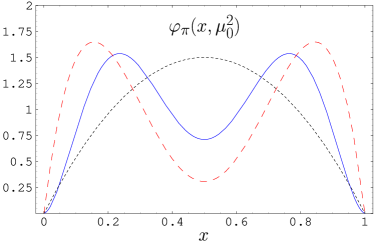
Figure 2: Comparison of selected pion DAs denoted by obvious acronyms: $\varphi_{\text{as}}$ (dotted line), $\varphi_{\text{CZ}}$ (dashed line) Chernyak and Zhitnitsky (1984), and $\varphi_{\text{BMS}}$ (solid line) Bakulev et al. (2001), defined by Eq. (12) in conjunction with (19). All DAs are normalized at the same scale ${\mu_{0}^{2}}\approx 1$ GeV².

The nonperturbative input, alias the pion DA at the initial normalization scale ${\mu_{0}^{2}}$, $\varphi_{\pi}(x,\mu_{0}^{2})$, will be expressed as an expansion over Gegenbauer polynomials which form an eigenfunctions decomposition, having recourse to a convenient representation which separates the $x$ and $\mu^{2}$ dependence (a detailed exposition can be found in Stefanis (1999)). Then, the pion DA at the initial scale ${\mu_{0}^{2}}$ reads

$$\varphi_{\pi}(x,\mu_{0}^{2})=6x(1-x)\left[1+a_{2}({\mu_{0}^{2}})\,C_{2}^{3/2}(2x-1)+a_{4}({\mu_{0}^{2}})\,C_{4}^{3/2}(2x-1)+\ldots\right]\,,$$ (12)

with all nonperturbative information being encapsulated in the coefficients $a_{n}$. These coefficients will be taken from a QCD sum-rules calculation employing nonlocal condensates Bakulev et al. (2001); Bakulev et al. (2003a), and we refer the reader to these works for more details. Here we only use the results obtained there. We found at ${\mu_{0}^{2}}=1.35$ GeV² and for a quark virtuality of $\lambda_{q}^{2}=0.4$ GeV²:

$$\begin{array}[]{lll}a_{0}=1&\quad\quad\quad a_{2}=0.19&\quad\quad\quad a_{4}=-0.13\\ a_{6}=5\times 10^{-3}&\quad\quad\quad a_{8}=4\times 10^{-3}&\quad\quad\quad a_{10}=4\times 10^{-3}\,.\end{array}$$ (15)

One appreciates that all Gegenbauer coefficients with $n>4$ are close to zero and can therefore be neglected. Hence, to model the pion DA, it is sufficient to keep only the first two coefficients, which we display below in comparison with those for the asymptotic DA and the CZ Chernyak and Zhitnitsky (1984) model after 2-loop evolution to the reference scale ${\mu_{0}^{2}}=1$ GeV², i.e.,

$$\begin{array}[]{rllll}\varphi_{\text{as}}:&a_{n}=0\>,n\geq 2&&&\quad{\mu_{0}^{2}}=\mu_{\text{F}}^{2},\\ \varphi_{\text{BMS}}:&a_{n}=0\>,n>4&\quad a_{2}=0.20&\quad a_{4}=-0.14&\quad{\mu_{0}^{2}}=1~{}\text{GeV}^{2}\\ \varphi_{\text{CZ}}:&a_{n}=0\>,n>2&\quad a_{2}=0.56&&\quad{\mu_{0}^{2}}=1~{}\text{GeV}^{2}\quad\,.\end{array}$$ (19)

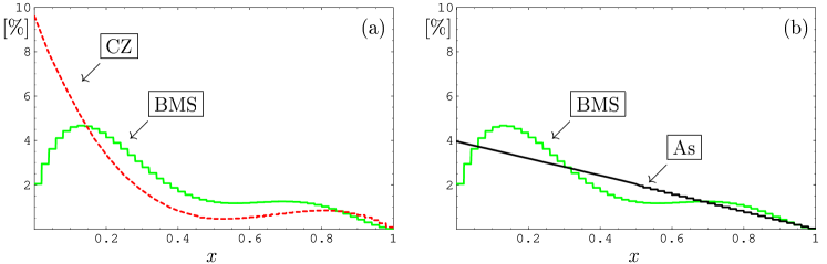
Figure 3: Percentage distribution (see text) of the first inverse moment in $x$ of the BMS model DA Bakulev et al. (2001) in comparison with the CZ one Chernyak and Zhitnitsky (1984) (a) and the asymptotic DA (b).

The shapes of these DAs are displayed in Fig. 2.

At this point some important remarks and observations are in order.

• The BMS pion DA, though doubly-peaked, has its endpoints $x\to 0$ and $x\to 1$ strongly suppressed due to the nonlocality parameter $\lambda_{q}^{2}$. Hence, fears frequently expressed in the literature that double-humped pion DAs should be avoided because they may emphasize the endpoint region, where the use of perturbation theory is unjustified, are unfounded.

• The BMS pion DA approaches asymptotically $\varphi_{\text{as}}$ in the endpoints from below, whereas $\varphi_{\text{CZ}}$ approaches the asymptotic limit from above, which means that the endpoint behavior of the latter is dangerous until very large values of $Q^{2}$. It is well-known Mueller (1997); Stefanis et al. (1999); Stefanis (1999) that in the endpoint region $x\to 1$ the spectator quark in the hard process, carrying the small longitudinal momentum fraction $\bar{x}$, can “wait” for a long time until it exchanges a soft gluon with the struck quark to fit again into the final pion wave function. As a result, a strong Sudakov suppression Li and Sterman (1992) is needed in that case in order to justify the use of perturbation theory. In contrast, the endpoint behavior of the BMS DA is not controversial because, though doubly peaked, it does not emphasize the endpoint regions. Even more, as Fig. 3 shows by plotting the first inverse moment $\langle x^{-1}\rangle_{\pi}$, calculated as $\int_{x}^{x+0.02}\varphi_{\pi}(x)x^{-1}dx$ and normalized to $100\%$ ($y$-axis), the BMS DA receives in this region even less contributions than the asymptotic DA, as we explained above.

• By the same token, the Sudakov suppression of the endpoint region of the BMS DA is less crucial compared to endpoint-concentrated DAs. The implementation of Sudakov corrections using the analytic factorization scheme was considered in technical detail in Stefanis et al. (1999) for the case of the asymptotic pion DA. Such an analysis for the BMS DA is more involved and will be conducted in a future publication.

• The deep reason for the failure of the CZ DA was provided in Mikhailov and Radyushkin (1989, 1992); Radyushkin (1997). The condensate terms in the CZ sum rules are strongly peaked at the endpoints $x\to 0$ and $x\to 1$, the reason being that the vacuum quark distribution in the longitudinal momentum fractions is approximated by a $\delta$-function $\delta(x)$ and its derivatives. For that reason, the condensate terms, i.e., the nonperturbative contributions to the sum rule, force the pion DA to be endpoint-concentrated, with the perturbative loop contribution proportional to $x(1-x)$ being insufficient to compensate these two sharp peaks at $x=0$ and $x=1$. Allowing for a smooth distribution in the longitudinal momentum for the vacuum quarks, i.e., using nonlocal condensates in the QCD sum rules (as done in the derivation of the BMS pion DA), the endpoint regions of the extracted DA are suppressed, despite the fact that its shape is doubly peaked.

  

  Figure 4: Light-cone sum-rule predictions for $Q^{2}F_{\gamma^{*}\gamma\to\pi}(Q^{2})$ in comparison with the CELLO (diamonds, Behrend et al. (1991)) and the CLEO (triangles, Gronberg et al. (1998)) experimental data evaluated with the twist-4 parameter value $\delta_{\text{Tw-4}}^{2}=0.19$ GeV² Bakulev et al. (2003b, 2004). The predictions shown correspond to the following pion DA models: $\varphi_{\text{CZ}}$ (upper dashed line) Chernyak and Zhitnitsky (1984), BMS-“bunch” (shaded strip) Bakulev et al. (2001), two instanton-based models, viz., Petrov et al. (1999) (dotted line) and Praszalowicz and Rostworowski (2001a) (dashed-dotted line), and the asymptotic pion DA $\varphi_{\text{as}}$ (lower dashed line) Efremov and Radyushkin (1980a); Lepage and Brodsky (1979). A recent transverse lattice result Dalley and van de Sande (2002) is very close to the dash-dotted line, but starts to be closer to the center of the BMS strip for $Q^{2}\geq 6$ GeV² .

• The endpoint behavior of the pion DA is the route cause why the pion-photon transition form factor—which in LO is purely electromagnetic—calculated with the CZ pion DA was found Kroll and Raulfs (1996) to overshoot the CLEO data. More recently, the analysis of the CLEO data using light-cone sum rules Khodjamirian (1999); Schmedding and Yakovlev (2000); Bakulev et al. (2003b, 2004) has excluded the CZ pion DA at the 4$\sigma$ confidence level, while the BMS DA was found to be inside the 1$\sigma$ error ellipse (for $\lambda_{q}^{2}=4$ GeV²), whereas even the asymptotic DA was also excluded by the CLEO data at the 3$\sigma$ level. These quoted findings are reflected in the behavior of the predictions for the pion-photon transition form factor displayed in Fig. 4, which is based on the corrected version of Bakulev et al. (2001) (the displayed strip is therefore slightly different from that in Bakulev et al. (2003c)).

To make these statements more transparent, let us define the DA profile deviation factor

$$\Delta_{\varphi}\equiv\frac{\langle x^{-1}\rangle^{\rm\varphi}_{\pi}}{\langle x^{-1}\rangle^{\rm As}_{\pi}}=1+a_{2}+a_{4}+\ldots$$ (20)

which quantifies the deviation of a model DA from the asymptotic one and supply its value in Table 5 for several pion DAs suggested in the literature in comparison with the constraints from the experimental data and theoretical calculations. Reading this Table in conjunction with Fig. 4, one comes to the conclusion that the BMS “bunch” provides the best agreement with the CLEO and CELLO experimental constraints, being also in compliance with various theoretical constraints and lattice calculations.

Table 1: Estimates for the Gegenbauer coefficients and the DA profile deviation factor $\Delta_{\varphi}$ up to polynomial order 4 for the asymptotic, the BMS, and the CZ DAs compared with constraints derived from light-cone sum rules (LCSR), QCD sum rules with nonlocal condensates (NL QCD SR) for the DA and the inverse moment $\langle{x^{-1}}\rangle$, and by analyzing the CLEO data. Also shown are the corresponding entries for instanton-based models (ADT, PPRWG, PR) and those associated with a transverse-lattice calculation—labelled Lattice. All values displayed are normalized at the scale $\mu^{2}=1.35$ GeV², corresponding to the scale of NL QCD SRs.

DA models/methods	$a_{2}$	$a_{4}$	$a_{2}+a_{4}$	$a_{2}-a_{4}$	$\Delta_{\varphi}$
As	0	0	$0$	$0$	$1$
BMS	$0.19$	$-0.13$	$0.06$	$0.32$	$1.06$
CZ	$0.52$	$0$	$0.52$	$0.52$	$1.52$
PPRWG Petrov et al. (1999)	$0.042$	$0.006$	$0.05$	$0.04$	$1.05$
PR Praszalowicz and Rostworowski (2001b)	$0.09$	$-0.02$	$0.07$	$0.10$	$1.07$
ADT Anikin et al. (2000)	$0.05$	$-0.04$	$0.01$	$0.09$	$1.01$
Lattice Dalley and van de Sande (2002)	$0.08$	$0.02$	$0.10$	$0.06$	$1.10$
LCSRs Bijnens and Khodjamirian (2002)	$[0.07,0.37]$	—	—	—	$1.22\pm 0.15$
NL QCD SRs for DA Bakulev et al. (2001)	$[0.13,0.25]^{a}$	$[-0.04,-0.21]^{a}$	$[+0.02,+0.09]$	$[+0.18,+0.46]$	$1.06\pm 0.04$
NL QCD SR for $\langle{x^{-1}}\rangle$ Bakulev et al. (2001)	—	—	$[+0.00,+0.20]$	—	$1.10\pm 0.10$
CLEO $1\sigma$-limits Bakulev et al. (2004)	$[0.15,0.43]^{a}$	$[-0.60,-0.04]^{a}$	$[-0.21,+0.15]$	$[+0.21,+1.00]$	$0.97\pm 0.18$
CLEO $2\sigma$-limits Bakulev et al. (2004)	$[0.11,0.47]^{a}$	$[-0.71,+0.07]^{a}$	$[-0.31,+0.25]$	$[+0.07,+1.14]$	$0.97\pm 0.28$
CLEO $3\sigma$-limits Bakulev et al. (2004)	$[0.07,0.51]^{a}$	$[-0.82,+0.19]^{a}$	$[-0.41,+0.35]$	$[-0.07,+1.28]$	$0.97\pm 0.38$

III.2 Perturbative NLO evolution

Let us now discuss how the pion DA evolves at NLO using first standard perturbation theory to be followed by analogous considerations within APT. The evolution of the distribution amplitude (12) proceeds along the lines outlined in Appendix C. Taking into account only the first two Gegenbauer coefficients and LO evolution, one obtains

$$\varphi_{\pi}^{\text{LO}}(x,\mu_{\text{F}}^{2})=6x(1-x)\left[1+a_{2}^{\text{D,LO}}(\mu_{\text{F}}^{2})\,C_{2}^{3/2}(2x-1)+a_{4}^{\text{D,LO}}(\mu_{\text{F}}^{2})\,C_{4}^{3/2}(2x-1)\right]\,,$$ (21)

where $a_{2}^{\text{D,LO}}(\mu_{\text{F}}^{2})$ and $a_{4}^{\text{D,LO}}(\mu_{\text{F}}^{2})$ are given by (135) taking recourse to (131), and D denotes “diagonal”, while ND below stands for “nondiagonal”.

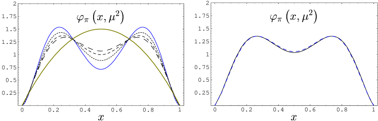
Figure 5: The left panel shows the effect of the LO diagonal part of the evolution equation, Eq. (21), on the BMS DA. The convex solid line denotes the asymptotic profile of the pion DA, the other solid one stands for $\varphi_{\text{BMS}}^{\text{LO}}(x)$ at 1 GeV², while the broken lines represent $\varphi_{\text{BMS}}^{\text{LO}}(x)$ at 4, 20, and 100 GeV² (with the larger scale corresponding also to the larger value of the DA at the middle point). Right panel: Comparison of $\varphi_{\text{BMS}}^{\text{LO}}$ (Eq. (21)—solid line) and $\varphi_{\text{BMS}}^{\text{NLO}}$ (Eq. (22)—dashed line) at 20 GeV² to illustrate the effect of NLO evolution.

On the other hand, the solution of the NLO evolution equation takes the form

$$\varphi_{\pi}^{\text{NLO}}(x,\mu_{\text{F}}^{2})=\varphi_{\pi}^{\text{D,NLO}}(x,\mu_{\text{F}}^{2})+\frac{\alpha_{s}(\mu_{\text{F}}^{2})}{4\pi}\,\varphi_{\pi}^{\text{ND,NLO}}(x,\mu_{\text{F}}^{2})\,,$$ (22a)

where

$$\varphi_{\pi}^{\text{D,NLO}}(x,\mu_{\text{F}}^{2})=6x(1-x)\left[1+\sum_{n=2,4}a_{n}^{\text{D,NLO}}(\mu_{\text{F}}^{2})\,C_{n}^{3/2}(2x-1)\right]$$ (22b)

and

$$\varphi_{\pi}^{\text{ND,NLO}}(x,\mu_{\text{F}}^{2}) = 6x(1-x){\sum_{n\geq 2}}^{\prime}a_{n}^{\text{ND,NLO}}(\mu_{\text{F}}^{2})\,C_{n}^{3/2}(2x-1)\,.$$ (22c)

The coefficients $a_{n}^{\text{D,NLO}}(\mu_{\text{F}}^{2})$ and $a_{n}^{\text{ND,NLO}}(\mu_{\text{F}}^{2})$ are given in (136b) and (136c), respectively, by employing (132), while ${\sum}^{\prime}$ denotes the sum over even indices only. Note that, although the input DA, $\varphi_{\pi}(x,{\mu_{0}^{2}})$, was parameterized by only two Gegenbauer coefficients $a_{2}$ and $a_{4}$, higher harmonics also appear due to the nondiagonal nature of the NLO evolution. The effect of the inclusion of the LO diagonal part of the evolution kernel is important, as one sees from the left part of Fig. 5, which shows this effect for the BMS pion DA.

On the other hand, from the right part of Fig. 5, we deduce that the NLO nondiagonal evolution is rather small. We note that in the above computation the exact two-loop expression for $\alpha_{s}$ Magradze (1999) in the $\overline{\text{MS}\vphantom{{}^{1}}}$ -scheme ($\Lambda_{\text{QCD}}=410$ MeV, $N_{f}=3$) was employed, cf. (68), in which matching at the heavy-flavor thresholds $M_{4}=1.3$ GeV and $M_{5}=4.3$ GeV (with $M_{1}=M_{2}=M_{3}=0$) has been employed Shirkov and Mikhailov (1994). A discussion of the relation of this exact solution to the usual approximation, promoted by the Particle Data Group Hagiwara et al. (2002), has recently been given in Bakulev et al. (2004) (see also Appendix C).

IV Pion form factor at NLO: Analytic results

The NLO results for the hard-scattering amplitude $T_{\text{H}}$ are summarized in Appendix A. Setting in (4) $\mu_{\text{F}}^{2}=Q^{2}$ and taking into account the NLO evolution of the pion DA $\varphi$ via (22), we obtain from (3)

$$F_{\pi}^{\text{Fact}}(Q^{2};\mu_{\text{R}}^{2})=F_{\pi}^{\text{LO}}(Q^{2};\mu_{\text{R}}^{2})+F_{\pi}^{\text{NLO}}(Q^{2};\mu_{\text{R}}^{2})\,,$$ (23)

where the LO term is given by

$$F_{\pi}^{\text{LO}}(Q^{2};\mu_{\text{R}}^{2}) = \alpha_{s}(\mu_{\text{R}}^{2})\,{\cal F}_{\pi}^{\text{LO}}(Q^{2})$$ (24)

$$Q^{2}{\cal F}_{\pi}^{\text{LO}}(Q^{2}) \equiv 8\,\pi\,f_{\pi}^{2}\,\left[1+a_{2}^{\text{D,NLO}}(Q^{2})+a_{4}^{\text{D,NLO}}(Q^{2})\right]^{2}$$ (25)

and the calligraphic designations denote quantities with their $\alpha_{s}$-dependence pulled out. In order to make a distinction between the contributions stemming from the diagonal and the nondiagonal parts of the NLO evolution equation of the pion DA, we express the NLO correction to the form factor in the form

$$F_{\pi}^{\text{NLO}}(Q^{2};\mu_{\text{R}}^{2})=\frac{\alpha_{s}^{2}(\mu_{\text{R}}^{2})}{\pi}\,\left[{\cal F}_{\pi}^{\text{D,NLO}}(Q^{2};\mu_{\text{R}}^{2})+{\cal F}_{\pi}^{\text{ND,NLO}}(Q^{2};N_{\text{Max}}=\infty)\right]$$ (26)

and write the diagonal contribution

$${\cal F}_{\pi}^{\text{D,NLO}}(Q^{2};\mu_{\text{R}}^{2}) \equiv b_{0}\,{\cal F}_{\pi}^{(1,\beta)}(Q^{2};\mu_{\text{R}}^{2})+C_{\text{F}}{\cal F}_{\pi}^{(1,\text{F})}(Q^{2})+C_{\text{G}}{\cal F}_{\pi}^{(1,\text{G})}(Q^{2})$$ (27)

as a color decomposition (in correspondence with (104)) in terms of

$$Q^{2}{\cal F}_{\pi}^{(1,\beta)}(Q^{2};\mu_{\text{R}}^{2}) = 2\,\pi\,f_{\pi}^{2}\,\left[\displaystyle\frac{5}{3}+\frac{3+\displaystyle(43/6)a_{2}^{\text{D,NLO}}(Q^{2})+(136/15)a_{4}^{\text{D,NLO}}(Q^{2})}{1+a_{2}^{\text{D,NLO}}(Q^{2})+a_{4}^{\text{D,NLO}}(Q^{2})}-\ln\frac{Q^{2}}{\mu_{\text{R}}^{2}}\right]$$ (28a)

$$\times\left[1+a_{2}^{\text{D,NLO}}(Q^{2})+a_{4}^{\text{D,NLO}}(Q^{2})\right]^{2}\,,$$

$$Q^{2}{\cal F}_{\pi}^{(1,\text{F})}(Q^{2}) = 2\,\pi\,f_{\pi}^{2}\,\left\{-\frac{71}{6}-a_{2}^{\text{D,NLO}}(Q^{2})\left[\frac{497}{36}-\frac{161}{24}\,a_{2}^{\text{D,NLO}}(Q^{2})\right]\right.$$

$$\left.\qquad\quad-\ a_{4}^{\text{D,NLO}}(Q^{2})\left[\frac{1123}{450}-\frac{9793}{300}\,a_{2}^{\text{D,NLO}}(Q^{2})-\frac{1387}{50}\,a_{4}^{\text{D,NLO}}(Q^{2})\right]\right\}\,,$$

and

$$Q^{2}{\cal F}_{\pi}^{(1,\text{G})}(Q^{2}) = 2\,\pi\,f_{\pi}^{2}\,\left\{-0.67+a_{2}^{\text{D,NLO}}(Q^{2})\left[18.70+16.35\,a_{2}^{\text{D,NLO}}(Q^{2})\right]\right.$$

$$\left.\qquad\quad+\ a_{4}^{\text{D,NLO}}(Q^{2})\left[24.23+36.76\,a_{2}^{\text{D,NLO}}(Q^{2})+20.26\,a_{4}^{\text{D,NLO}}(Q^{2})\right]\right\}\,,$$

where the superscripts F and G refer to the color factors $C_{\text{F}}$ and $C_{\text{G}}=C_{\text{F}}-C_{\text{A}}/2$, respectively. Note that for the matter of calculational convenience, we also display the sum of these two terms (cf. Eq. (108)):

$$Q^{2}{\cal F}_{\pi}^{(1,\text{FG})}(Q^{2}) = 2\,\pi\,f_{\pi}^{2}\,\left\{-15.67-a_{2}^{\text{D,NLO}}(Q^{2})\left[21.52-6.22\,a_{2}^{\text{D,NLO}}(Q^{2})\right]\right.$$

$$\left.-\ a_{4}^{\text{D,NLO}}(Q^{2})\left[7.37-37.40\,a_{2}^{\text{D,NLO}}(Q^{2})-33.61\,a_{4}^{\text{D,NLO}}(Q^{2})\right]\right\}\,.$$

On the other hand, the nondiagonal term reads

$$Q^{2}{\cal F}_{\pi}^{\text{ND,NLO}}(Q^{2};N_{\text{Max}})=4\pi\,f_{\pi}^{2}\left[1+a_{2}^{\text{D,NLO}}(Q^{2})+a_{4}^{\text{D,NLO}}(Q^{2})\right]\sum_{k=2}^{N_{\text{Max}}}{}^{\prime}a_{k}^{\text{ND,NLO}}(Q^{2})\,,$$ (30)

where $N_{\text{Max}}$ denotes the maximal number of Gegenbauer harmonics taken into account in order to achieve the desired accuracy.

As it was shown in Ref. Melić et al. (1999), the effects of the LO DA evolution are crucial. In order to investigate the importance of the NLO DA evolution, we compare the predictions obtained using the complete NLO results, given above, with those derived by employing only the LO DA evolution via (21). The corresponding expressions in this latter case follow from those above by performing the replacements

$$a_{n}^{\text{D,NLO}}\to a_{n}^{\text{D,LO}}\qquad\text{and}\qquad a_{n}^{\text{ND,NLO}}\to 0\,,$$ (31)

so that the contribution ${\cal F}_{\pi}^{\text{ND,NLO}}(Q^{2};\mu_{\text{R}}^{2})$ is absent. Introducing the notation

$$\widetilde{\cal F}_{\pi}^{i}\equiv{\cal F}_{\pi}^{i}|_{\text{LO DA evolution}}\,,$$ (32)

we analyze the relative importance of the various contributions (LO, NLO, and Local Duality (LD) part—see Sec. VII.3) by defining the following ratios

$$R\left(Q^{2},N_{\text{Max}}\right) = \frac{{\cal F}_{\pi}^{\text{LO}}\left(Q^{2}\right)+(\alpha_{s}/\pi){\cal F}_{\pi}^{\text{ND,NLO}}\left(Q^{2};N_{\text{Max}}\right)}{{\cal F}_{\pi}^{\text{LO}}\left(Q^{2}\right)+(\alpha_{s}/\pi){\cal F}_{\pi}^{\text{ND,NLO}}\left(Q^{2};N_{\text{Max}}\approx\infty\right)}\,;$$ (33)

$$\hat{R}\left(Q^{2},N_{\text{Max}}\right) = \frac{F_{\pi}^{\text{LD}}\left(Q^{2}\right)+\alpha_{s}{\cal F}_{\pi}^{\text{LO}}\left(Q^{2}\right)+(\alpha_{s}^{2}/\pi){\cal F}_{\pi}^{\text{ND,NLO}}\left(Q^{2};N_{\text{Max}}\right)}{F_{\pi}^{\text{LD}}\left(Q^{2}\right)+\alpha_{s}{\cal F}_{\pi}^{\text{LO}}\left(Q^{2}\right)+(\alpha_{s}^{2}/\pi){\cal F}_{\pi}^{\text{ND,NLO}}\left(Q^{2};N_{\text{Max}}\approx\infty\right)}\,;$$ (34)

$$R_{\text{mod}}\left(Q^{2}\right) = \frac{\widetilde{\cal F}_{\pi}^{\text{LO}}\left(Q^{2}\right)}{{\cal F}_{\pi}^{\text{LO}}\left(Q^{2}\right)+(\alpha_{s}/\pi){\cal F}_{\pi}^{\text{ND,NLO}}\left(Q^{2};N_{\text{Max}}\approx\infty\right)}\,;$$ (35)

$$\hat{R}_{\text{mod}}\left(Q^{2}\right) = \frac{F_{\pi}^{\text{LD}}\left(Q^{2}\right)+\alpha_{s}\widetilde{\cal F}_{\pi}^{\text{LO}}\left(Q^{2}\right)}{F_{\pi}^{\text{LD}}\left(Q^{2}\right)+\alpha_{s}{\cal F}_{\pi}^{\text{LO}}\left(Q^{2}\right)+(\alpha_{s}^{2}/\pi){\cal F}_{\pi}^{\text{ND,NLO}}\left(Q^{2};N_{\text{Max}}\approx\infty\right)}\,.$$ (36)

   

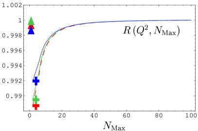
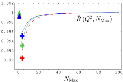
Figure 6: Left: The ratio $R\left(Q^{2},N_{\text{Max}}\right)$, defined in Eq. (33), for three different values of $Q^{2}$ as a function of $N_{\text{Max}}$. The blue dotted curve corresponds to $Q^{2}=2$ GeV², the green solid curve to $Q^{2}=10$ GeV², and the red dashed one to $Q^{2}=50$ GeV². Crosses of the same color represent the values of $R\left(Q^{2},N_{\text{Max}}=4\right)$, whereas triangles refer to $R_{\text{mod}}\left(Q^{2}\right)$, Eq. (35). Right: The same designations hold as for the left side, but now for the ratio $\hat{R}\left(Q^{2},N_{\text{Max}}\right)$ given by Eq. (34) and correspondingly for $\hat{R}_{\text{mod}}$—Eq. (36).

These ratios are displayed graphically in Fig. 6 for the BMS DA ($a_{2}({\mu_{0}^{2}})=0.2$, $a_{4}({\mu_{0}^{2}})=-0.14$) in the region $N_{\text{Max}}=4-100$. We infer from this figure that, adopting in our calculations an accuracy on the order of 99.5%, we can safely neglect the non-diagonal part of the NLO evolution equation and use for the pion form-factor computations to follow the approximate expression (omitting the superscript Approx)

$$F_{\pi}^{\text{Fact-Approx}}(Q^{2};\mu_{\text{R}}^{2})\equiv\alpha_{s}(\mu_{\text{R}}^{2})\,\tilde{\cal F}_{\pi}^{\text{LO}}(Q^{2};\mu_{\text{R}}^{2})+\frac{\alpha_{s}^{2}(\mu_{\text{R}}^{2})}{\pi}\,{\cal F}_{\pi}^{\text{D,NLO}}(Q^{2};\mu_{\text{R}}^{2})\,.$$ (37)

Actually, the difference between ${\cal F}_{\pi}^{\text{D,NLO}}(Q^{2};\mu_{\text{R}}^{2})$ and $\tilde{\cal F}_{\pi}^{\text{D,NLO}}(Q^{2};\mu_{\text{R}}^{2})$ is of the order of $\alpha_{s}(Q^{2})$, so that it is safe to use everywhere only the LO evolution. We have verified in our numerical calculations that the difference is indeed less than 1%.

V Setting the Renormalization Scheme and Scale

The choice of the expansion parameter represents the major ambiguity in the interpretation of the pQCD predictions because finite-order perturbative predictions depend unavoidably on the renormalization scale and scheme choice. If one could optimize the choice of the renormalization scale and scheme according to some sensible criteria, the size of the higher-order corrections, as well as the size of the expansion parameter, i.e., the QCD running coupling, could serve as sensible indicators for the convergence of the perturbative expansion. In what follows, we shall consider several scheme and scale-setting options.

V.1 $\overline{\text{MS}}$ scheme

The results we have presented in the previous subsection were obtained in the $\overline{\text{MS}\vphantom{{}^{1}}}$ renormalization (and factorization) scheme. Let us discuss the choice of the renormalization scale $\mu_{\text{R}}$ in some more detail. We see that in our NLO results, Eq. (26), this dependence is contained in the coupling constant $\alpha_{s}(\mu_{\text{R}}^{2})$ as well as in the NLO correction ${\cal F}_{\pi}^{(1,\beta)}$. The latter correction is proportional to the $b_{0}$ coefficient of the $\beta$ function and is $N_{f}$-dependent. Hence, a natural question arises: How can we determine the right value of $N_{f}$ in the form-factor expression?

We propose here to apply the following procedures.
(i) The first one concerns the standard choice $\mu_{\text{R}}^{2}=Q^{2}$ and suggests to shift $\mu_{\text{R}}^{2}$ at the heavy-quark threshold in order to ensure the continuity of the form factor according to

$$F_{\pi}^{\text{Fact}}(Q^{2})=\left\{\begin{array}[]{ll}F_{\pi}^{\text{Fact}}(Q^{2};\mu_{\text{R}}^{2}=Q^{2})\big{|}_{N_{f}=3}&\text{for}~{}Q^{2}\leq M_{4}^{2};\\ F_{\pi}^{\text{Fact}}(Q^{2};\mu_{\text{R}}^{2}=Q^{2}+\delta\mu^{2}_{4})\big{|}_{N_{f}=4}\vphantom{{}^{\Big{|}}}&\text{for}~{}\left\{\begin{array}[]{l}M_{4}^{2}\leq Q^{2}\\ Q^{2}+\delta\mu^{2}_{4}\leq M_{5}^{2}\end{array}\right.;\\ F_{\pi}^{\text{Fact}}(Q^{2};\mu_{\text{R}}^{2}=Q^{2}+\delta\mu^{2}_{4}+\delta\mu^{2}_{5})\big{|}_{N_{f}=5}\vphantom{{}^{\Big{|}}}&\text{for}~{}M_{5}^{2}\leq Q^{2}+\delta\mu^{2}_{4}\,.\end{array}\right.$$ (38f)

As a result, we have to fulfill the following matching conditions

$$F_{\pi}^{\text{Fact}}(M_{4}^{2};M_{4}^{2})\big{|}_{N_{f}=3} = F_{\pi}^{\text{Fact}}(M_{4}^{2};M_{4}^{2}+\delta\mu^{2}_{4})\big{|}_{N_{f}=4}\,;$$ (38g)

$$F_{\pi}^{\text{Fact}}(M_{5}^{2}-\delta\mu^{2}_{4};M_{5}^{2})\big{|}_{N_{f}=4} = F_{\pi}^{\text{Fact}}(M_{5}^{2}-\delta\mu^{2}_{4};M_{5}^{2}+\delta\mu^{2}_{5})\big{|}_{N_{f}=5}.\quad$$ (38h)

(ii) The second procedure addresses specifically the BLM scale setting $\mu_{\text{R}}^{2}=\mu_{\text{BLM}}^{2}$. In this case, the only problem is the small value of the BLM scale (see Table 2) due to the fact that the $b_{0}$-term is completely absent and $N_{f}$-dependent terms do not arise. Therefore, we propose to implement the BLM scale setting only above some minimal scale: $\mu_{\text{min}}$. Below this scale, which is in the range of the typical meson scales and hence only the light-quark sector ($N_{f}=3$) contributes, we fix $\mu_{\text{R}}^{2}=\mu_{\text{min}}^{2}$ and set $N_{f}=3$ using the ${\cal F}_{\pi}^{(1,\beta)}(Q^{2};\mu_{\text{min}}^{2})$-term in the form provided by (50)—more explanations will be given shortly.

The truncation of the perturbative series to a finite order introduces a residual dependence of the results on the scale $\mu_{\text{R}}$, while the inclusion of higher-order corrections decreases this dependence. Nonetheless, we are still left with an intrinsic theoretical ambiguity of the perturbative results. One can try to estimate the uncertainty entailed by this ambiguity (see, for example, Melić et al. (1999)) or choose the renormalization scale $\mu_{\text{R}}$ on the basis of some physical arguments.

The simplest and widely used choice for $\mu_{\text{R}}$ is to identify it with the large external scale, i.e., to set

$$\mu_{\text{R}}^{2}=Q^{2}\,,$$ (39)

the justification for adopting this choice being mainly a pragmatic one. However, physical arguments suggest that a more appropriate scale should be lower. Namely, since each external momentum entering an exclusive reaction is partitioned among many propagators of the underlying hard-scattering amplitude in the associated Feynman diagrams, the physical scales that control these processes are related to the average momentum flowing through the internal quark and gluon lines and are therefore inevitably softer than the overall momentum transfer. To treat this problem, several suggestions have been made in the literature. According to the so-called Fastest Apparent Convergence (FAC) procedure Grunberg (1980, 1984), the scale $\mu_{\text{R}}$ is determined by the requirement that the NLO coefficient in the perturbative expansion of the physical quantity in question vanishes which here means

$$F_{\pi}^{\text{NLO}}(Q^{2};\mu_{\text{R}}^{2}=\mu_{\text{FAC}}^{2})=0\,.$$ (40)

On the other hand, following the Principle of Minimum Sensitivity (PMS) Stevenson (1981a, b, 1982, 1984), one mimics locally the global independence of the all-order expansion by choosing the renormalization scale $\mu_{\text{R}}$ to coincide with the stationary point of the truncated perturbative series. In our case, this reads

$$\frac{d}{d\mu_{\text{R}}^{2}}\left[F_{\pi}^{\text{LO}}(Q^{2};\mu_{\text{R}}^{2})+F_{\pi}^{\text{NLO}}(Q^{2};\mu_{\text{R}}^{2})\right]\left|{}_{\displaystyle\mu_{\text{R}}^{2}=\displaystyle\mu_{\text{PMS}}^{2}}\right.=0\,.$$ (41)

In the Brodsky–Lepage–Mackenzie (BLM) procedure Brodsky et al. (1983a), all vacuum-polarization effects from the QCD $\beta$-function (i.e., the effects of quark loops) are absorbed into the renormalized running coupling by resumming the large ($b_{0}\alpha_{S}$)ⁿ terms giving rise to infrared renormalons. According to the BLM procedure, the renormalization scale best suited to a particular process at a given order of expansion can be, in practice, determined by demanding that the terms proportional to the $\beta$-function should vanish. This naturally connects to conformal field theory and we refer the interested reader to Braun et al. (2003) for a recent review. The optimization of the renormalization scale and scheme setting in exclusive processes by employing the BLM scale fixing was elaborated in Brodsky et al. (1998) and in references cited therein. The renormalization scales in the BLM method are “physical” in the sense that they reflect the mean virtuality of the gluon propagators involved in the Feynman diagrams. According to the BLM procedure, the renormalization scale is determined by the condition

$${\cal F}_{\pi}^{(1,\beta)}(Q^{2};\mu_{\text{R}}^{2}=\mu_{\text{BLM}}^{2})=0\,.$$ (42)

For calculational convenience, we express $\mu_{\text{R}}^{2}$ in terms of $Q^{2}$:

$$\mu_{\text{R}}^{2}=a(Q^{2})\;Q^{2}$$ (43)

and proceed to calculate this quantity in the above-mentioned scale-setting schemes. Then, the FAC procedure leads to

$$a_{\text{FAC}}(Q^{2}) = \exp\left[-\frac{5}{3}-\frac{3+\displaystyle(43/6)a_{2}^{\text{D,NLO}}(Q^{2})+(136/15)a_{4}^{\text{D,NLO}}(Q^{2})}{1+a_{2}^{\text{D,NLO}}(Q^{2})+a_{4}^{\text{D,NLO}}(Q^{2})}\right.$$ (44)

$$\left.\qquad-\frac{4}{b_{0}}\,\frac{{\cal F}_{\pi}^{(1,\text{FG})}(Q^{2})+{\cal F}_{\pi}^{\text{ND,NLO}}(Q^{2})}{{\cal F}_{\pi}^{\text{LO}}(Q^{2})}\right]\,,$$

which can be related to the PMS procedure via

$$a_{\text{PMS}}(Q^{2}) = e^{-c_{1}/2}a_{\text{FAC}}(Q^{2})$$ (45)

with $c_{1}\equiv b_{1}/b_{0}^{2}$. This value corresponds to the stationary point (the maximum) of the NLO prediction for $F_{\pi}^{\text{Fact}}$.

On the other hand, for the BLM scale one obtains

$$\mu_{\text{BLM}}^{2}=a_{\text{BLM}}(Q^{2})\,Q^{2}\,,$$ (46a)

where

$$a_{\text{BLM}}(Q^{2})=\exp\left[\displaystyle-\frac{5}{3}-\frac{3+\displaystyle(43/6)a_{2}^{\text{D,NLO}}(Q^{2})+(136/15)a_{4}^{\text{D,NLO}}(Q^{2})}{1+a_{2}^{\text{D,NLO}}(Q^{2})+a_{4}^{\text{D,NLO}}(Q^{2})}\right]\,.$$ (46b)

Table 2: Scales $\mu_{\text{PMS}}$, $\mu_{\text{FAC}}$, $\mu_{\text{BLM}}$, and $\mu_{V}$ for the asymptotic, the BMS, and the CZ DAs.

DA	$Q^{2}/\mu_{\text{FAC}}^{2}$	$Q^{2}/\mu_{\text{PMS}}^{2}$	$Q^{2}/\mu_{\text{BLM}}^{2}$	$Q^{2}/\mu_{V\vphantom{{}_{|}}}^{2}$	$Q^{2}$
As	$\displaystyle 18$	$\displaystyle 27$	$\displaystyle 106$	$\displaystyle 20$	any
BMS	$\displaystyle 16-20$	$\displaystyle 24-29$	$\displaystyle 105-117$	$\displaystyle 20-22$	$1-50$ GeV2
CZ	$\displaystyle 146-62$	$\displaystyle 217-92$	$\displaystyle 475-278$	$\displaystyle 90-52$	$1-50$ GeV2

The values of the scales $\mu_{\text{PMS}}$, $\mu_{\text{FAC}}$, and $\mu_{\text{BLM}}$ for the asymptotic, the CZ, and the BMS DAs, defined in (19), are listed in Table 2. One notices that the BLM scale is rather low for all considered DAs. This makes its applicability at experimentally accessible $Q^{2}$ values rather questionable. But it is possible to improve this scale-setting procedure in the following way.

First of all, let us rewrite the BLM prescription in the more suggestive form

$$\Bigg{\{}F_{\pi}(Q^{2};\mu_{\text{R}}^{2}),{\cal F}_{\pi}^{(1,\beta)}(Q^{2};\mu_{\text{R}}^{2})=\frac{1}{4}{\cal F}_{\pi}^{\text{LO}}(Q^{2})\ln\left[\frac{\mu_{\text{R}}^{2}}{\mu_{\text{BLM}}^{2}(Q^{2})}\right]\Bigg{\}}\stackrel{{\scriptstyle\text{BLM}}}{{\Rightarrow}}$$

(47)

$$\qquad\Big{\{}F_{\pi}(Q^{2};\mu_{\text{BLM}}^{2}(Q^{2})),{\cal F}_{\pi}^{(1,\beta)}(Q^{2};\mu_{\text{BLM}}^{2}(Q^{2}))=0\Big{\}}\,.$$

It becomes evident that when the BLM scale yields $\alpha_{s}$ values close to unity, perturbation theory breaks down. To avoid this happening, one can, of course, introduce ad hoc a cutoff for $\alpha_{s}$, operative, say, above $0.5-0.6$, or one can “freeze” $\alpha_{s}$ at low $Q^{2}$ scales to some finite value by introducing an effective gluon mass Ji and Amiri (1990); Brodsky et al. (1998). Still another possibility is to use the analytic coupling Shirkov and Solovtsov (1997), as done in Stefanis et al. (1999, 2000) (see next section).

In order to protect the BLM scale from intruding into the forbidden nonperturbative soft region, where perturbation theory becomes invalid, one can make use of a minimum scale, $\mu_{\text{min}}$, based on the grounds of QCD factorization theorems and the OPE, as applied for instance in Korchemsky (1989a, b); Gellas et al. (1997); Stefanis (1998) and also in Braun et al. (2000):

$$\mu^{2}_{\text{min}} \geq {\mu_{0}^{2}}\,.$$ (48)

Here ${\mu_{0}^{2}}$ stands for a typical nonperturbative (hadronic) scale in the range $[0.4-1.5]$ GeV² and corresponds roughly to the inverse distance at which the parton and hadron representations have to match each other. Note that the smaller $\mu_{\text{min}}^{2}$ is chosen, the deeper the endpoint region $x\to 1$ can be explored for smaller values of $Q^{2}$. It is intuitively clear that the typical parton virtuality in the (hard) Feynman diagrams—let us call it $\mu_{q}^{2}$—should not become less than its counterpart in the pion bound state: $\mu_{\pi}^{2}$. Because the latter is linked to the scale ${\mu_{0}^{2}}$, the scale $\mu_{\text{min}}^{2}$ should be limited from below by this scale. Consequently, we assume that the following hierarchy of scales—partonic (i.e., perturbative) and hadronic (i.e., nonperturbative)—holds:

$$\lambda_{q}^{2}<{\mu_{0}^{2}}\leq\mu_{q}^{2}\leq\mu_{\text{R-scheme}}^{2}\,.$$ (49)

Then, if $\mu^{2}_{\text{BLM}}<{\mu_{0}^{2}}$, one obtains instead of Eq. (47), the IR protected version (termed in our analysis $\overline{\text{BLM}\vphantom{{}^{1}}}$ prescription)

$$\Big{\{}F_{\pi}\left[Q^{2},\mu_{\text{BLM}}^{2}(Q^{2})\right],{\cal F}_{\pi}^{(1,\beta)}\left[Q^{2},\mu_{\text{BLM}}^{2}(Q^{2})\right]=0\Big{\}}\stackrel{{\scriptstyle\text{$\overline{\text{BLM}\vphantom{{}^{1}}}${ }}}}{{\Rightarrow}}$$

(50)

$$\left\{F_{\pi}(Q^{2};\mu_{\text{min}}^{2}),{\cal F}_{\pi}^{(1,\beta)}(Q^{2};\mu_{\text{min}}^{2})=\frac{1}{4}{\cal F}_{\pi}^{\text{LO}}(Q^{2})\ln\left(\frac{\mu_{\text{min}}^{2}}{\mu_{\text{BLM}}^{2}(Q^{2})}\right)\right\}\,.$$

This modification of the BLM scale setting enables us to treat the problem of the $N_{f}$-dependence of the $\beta$ function in the term ${\cal F}_{\pi}^{(1,\beta)}(Q^{2};\mu_{\text{R}}^{2})$ without any further assumptions or modifications. Because of the fact that the scale $\mu_{\text{R}}^{2}$ is now bounded from below by (48), one is not faced with ambiguities related to the variation of the number of active flavors $N_{f}$ due to heavy-quark thresholds in the $b_{0}$ coefficient entering ${\cal F}_{\pi}^{(1,\beta)}(Q^{2};\mu_{\text{R}}^{2})$. According to this, we set $N_{f}=3$ for $\mu_{\text{R}}^{2}=\mu_{\text{min}}^{2}$, whereas for $\mu_{\text{R}}^{2}=\mu_{\text{BLM}}^{2}>\mu_{\text{min}}^{2}$ there is no ambiguity by virtue of ${\cal F}_{\pi}^{(1,\beta)}(Q^{2};\mu_{\text{BLM}}^{2})=0$. Therefore, the bona fide BLM scale setting reads

$$\mu_{\text{$\overline{\text{BLM}\vphantom{{}^{1}}}${ }}}=\mbox{max}\left\{\mu_{\text{BLM}},\mu_{\text{min}}\right\}\,,$$ (51)

where $\mu_{\text{min}}$ will be specified later on in connection with the soft part of the form factor.

V.2 $\alpha_{V}$ scheme

The self-consistency of perturbation theory implies that the difference in the calculation to order $n$ of the same physical quantity in two different schemes must be of order $n+1$. This means that relations among different physical observables must be independent of the renormalization scale and scheme conventions to any fixed order of perturbation theory. In Ref. Brodsky and Lu (1995) it was argued that by applying the BLM scale-fixing procedure to perturbative predictions of two observables in, for example, the $\overline{\text{MS}\vphantom{{}^{1}}}$ -scheme, and then algebraically eliminating $\alpha_{\overline{\text{MS}}}$, one can link to each other any perturbatively calculable observables without scale and scheme ambiguity. Within this approach, the choice of the BLM scale ensures that the resulting “commensurate scale relation” is independent of the choice of the intermediate renormalization scheme employed. On these grounds, Brodsky et al. in Brodsky et al. (1998) have analyzed several exclusive hadronic amplitudes in the $\alpha_{V}$ scheme, in which the effective coupling $\alpha_{V}(\mu^{2})$ is defined by utilizing the heavy-quark potential $V(\mu^{2})$. The $\alpha_{V}$ scheme is a “natural”, physically motivated scheme, which by definition, automatically incorporates vacuum polarization effects due to the fermion-antifermion pairs into the coupling. The $\mu_{V}^{2}$ scale which then appears in the argument of the $\alpha_{V}$ coupling reflects the mean virtuality of the exchanged gluons. Furthermore, since $\alpha_{V}$ is an effective running coupling defined by virtue of a physical quantity, it must be finite at low momenta, and, therefore, an appropriate parameterization of the low-energy region should, in principle, be included.

The scale-fixed relation between the couplings $\alpha_{\overline{\text{MS}}}$ and $\alpha_{V}$ is given by Brodsky et al. (1998)

$$\alpha_{s}(\mu_{\text{BLM}}^{2})=\alpha_{V}(\mu_{V}^{2})\left[1+\frac{\alpha_{V}(\mu_{V}^{2})}{4\pi}\,\frac{8C_{\text{A}}}{3}+\cdots\right]\,,$$ (52a)

where

$$\mu_{V}^{2}=e^{5/3}\,\mu_{\text{BLM}}^{2}\,.$$ (52b)

The scales $\mu_{V}$ associated with selected pion DAs are included in Table 2.

Taking into account Eqs. (52), the NLO prediction for the pion form factor, given by Eqs. (23)–(30), gets modified as follows

$$\alpha_{s}(\mu_{\text{R}}^{2}) \rightarrow \alpha_{V}(\mu_{V}^{2})$$

$${\cal F}_{\pi}^{\text{D,NLO}}(Q^{2}) \rightarrow {\cal F}_{\pi}^{\text{D,NLO}}(Q^{2})={\cal F}_{\pi}^{(1,\text{FG})}(Q^{2})+2{\cal F}_{\pi}^{\text{LO}}(Q^{2})\,.$$

We are not going to present predictions in this scheme using the standard QCD coupling, as this would require the introduction of exogenous parameters, like an effective gluon mass, that cannot be fixed within the same approach but have to be taken from elsewhere. For such an application, we refer the interested reader to the analysis of Brodsky et al. (1998). The connection of Brodsky et al. (1998) to the analytic approach, which we will use below, was discussed in detail in Stefanis et al. (2000). Predictions for the pion form factor within the $\alpha_{V}$ scheme will be presented below in the context of Analytic Perturbation Theory.

VI Strong Running Coupling and Non-power Series Expansions

VI.1 One-loop case

In the one-loop approximation we have a rather simple renormalization-group (RG) equation for the running coupling constant:

$$\frac{d\ \alpha_{s}(\mu^{2})}{d\ln\mu^{2}} = \beta(\mu^{2})\,;$$ (54)

$$\beta_{\text{1-loop}}(\mu^{2}) = -b_{0}\left(\frac{\alpha_{s}^{2}(\mu^{2})}{4\pi}\right)$$ (55)

with $b_{0}$ given in Appendix A. The solution of this equation has the form

$$\alpha_{s}^{(1)}(Q^{2})=\frac{4\pi}{b_{0}\ln(Q^{2}/\Lambda^{2})}\,,$$ (56)

where $\Lambda\equiv\Lambda_{\text{QCD}}$ is the QCD scale parameter. A well-known problem here is the appearance of an IR pole at $Q^{2}=\Lambda^{2}$, which spoils the analyticity of the QCD running coupling.

In a series of papers Shirkov and Solovtsov (1997); Solovtsov and Shirkov (1998, 1999); Shirkov and Solovtsov (2001) Shirkov and Solovtsov introduced an analytic running coupling that avoids by construction the Landau singularity, thus generalizing earlier attempts by Radyushkin Radyushkin (1996) and Krasnikov and Pivovarov Krasnikov and Pivovarov (1982). To this end, they used the spectral representation for the QCD running coupling $\bar{\alpha}_{s}(Q^{2})$ (the bar over $\alpha_{s}$ means that the analyticity property is valid) and expressed it in the form

$$\bar{\alpha}_{s}(Q^{2})=\frac{1}{\pi}\int_{0}^{\infty}d\sigma\frac{\rho(\sigma)}{\sigma+Q^{2}-i\epsilon}$$ (57)

without subtractions due to the fact that the spectral density $\rho(\sigma)$ decreases as $1/\ln^{2}\sigma$ for large $\sigma$. The corresponding one-loop spectral density reads

$$\rho^{(1)}(\sigma)=\left(\frac{4\pi}{b_{0}}\right)\frac{\pi}{\ln^{2}(\sigma/\Lambda^{2})+\pi^{2}}$$ (58)

and provides the one-loop singularity-free coupling function

$$\bar{\alpha}_{s}^{(1)}(Q^{2}/\Lambda^{2})=\frac{4\pi}{b_{0}}\left[\frac{1}{\ln(Q^{2}/\Lambda^{2})}+\frac{\Lambda^{2}}{\Lambda^{2}-Q^{2}}\right]\,.$$ (59)

The first term on the RHS expresses the standard UV behavior of the invariant coupling, while the second one compensates the ghost pole at $Q^{2}=\Lambda^{2}$ and has a nonperturbative origin, being suppressed at $Q^{2}\to\infty$.

Let us now consider powers of the analytic coupling function. By performing an analytic continuation of the $k$-th power of the function (56) in the complex $Q^{2}$-plane, one determines the corresponding spectral functions $\rho_{k}^{(1)}(\sigma)$, ($k=1,2\ldots$):

$$\rho_{k}^{(1)}(\sigma)=\left(\frac{4\pi}{b_{0}}\right)^{k}{\textbf{Im}{}}\left(\frac{1}{\ln(-\sigma/\Lambda^{2})}\right)^{k}\,,$$ (60)

which in turn determine the analytic image ${\cal A}_{k}^{(1)}(Q^{2})$ of $\left[\alpha_{s}^{(1)}(Q^{2})\right]^{k}$, i.e.,

$${\cal A}_{k}^{(1)}(Q^{2})=\frac{1}{\pi}\int_{0}^{\infty}d\sigma\frac{\rho_{k}^{(1)}(\sigma)}{\sigma+Q^{2}-i\epsilon}\,.$$ (61)

For $k=1,2,\ldots$, we have

$${\cal A}_{k+1}^{(1)}(Q^{2})=-\left(\frac{4\pi}{kb_{0}}\right)\frac{\partial{\cal A}_{k}^{(1)}(Q^{2})}{\partial\ln Q^{2}}\quad\text{and}\quad{\cal A}_{1}^{(1)}(Q^{2})\equiv\bar{\alpha}_{s}^{(1)}(Q^{2}/\Lambda^{2})\,,$$ (62)

which for $k=1$ reduces to

$${\cal A}_{2}^{(1)}(Q^{2})=\left(\frac{4\pi}{b_{0}}\right)^{2}\left[\frac{1}{\ln^{2}(Q^{2}/\Lambda^{2})}+\frac{Q^{2}\Lambda^{2}}{\left(\Lambda^{2}-Q^{2}\right)^{2}}\right]\,.$$ (63)

Notice at this point some key properties of these functions:

• each ${\cal A}_{k}^{(1)}(Q^{2})$ with $k\geq 2$ tends to zero for $Q^{2}\to 0$;

• each ${\cal A}_{k}^{(1)}(Q^{2})$ has exactly $k-1$ zeros for $Q^{2}\in[0,\infty)$;

• when $Q^{2}\to\infty$, each ${\cal A}_{k}^{(1)}(Q^{2})\Big{|}_{Q^{2}\to\infty}\sim 1/\ln^{k}[Q^{2}]$ tends to 0.

These properties are universal in the sense that they do not depend on the loop order. The functions ${\cal A}_{k}(Q^{2})$ are used in the so-called Analytic Perturbation Theory Shirkov and Solovtsov (1997); Shirkov (1999); Gardi et al. (1998); Solovtsov and Shirkov (1999); Shirkov (2001a, c), where standard perturbative series, for example, for the Adler function

$$D^{\text{PT}}(Q^{2}) = N_{c}\sum_{f}e_{f}^{2}\left\{1+\frac{\alpha_{s}(Q^{2})}{\pi}+d_{1}\left[\frac{\alpha_{s}(Q^{2})}{\pi}\right]^{2}+\ldots\right\}$$ (64)

is recast into a non-power series expansion to obtain

$$D^{\text{APT}}(Q^{2}) = N_{c}\sum_{f}e_{f}^{2}\left[1+\frac{{\cal A}_{1}(Q^{2})}{\pi}+d_{1}\frac{{\cal A}_{2}(Q^{2})}{\pi^{2}}+\ldots\right]\,.$$ (65)

The one-loop expressions for ${\cal A}_{1}$ and ${\cal A}_{2}$ are given in (62) and (63), respectively.

VI.2 Two-loop case

In the two-loop case the situation is more complicated. The corresponding $\beta$-function reads

$$\beta_{\text{2-loop}}(\alpha)=\frac{-b_{0}\alpha^{2}}{4\pi}\left(1+\frac{b_{1}\alpha}{b_{0}\ 4\pi}\right)$$ (66)

with the first two beta coefficients given in Appendix A. Integrating the RG equation (54), we obtain the transcendental equation

$$L_{Q}=\frac{4\pi}{\alpha\left(L_{Q}\right)b_{0}}-c_{1}\ln\left(c_{1}+\frac{4\pi}{\alpha\left(L_{Q}\right)b_{0}}\right),\qquad c_{1}=\frac{b_{1}}{b_{0}^{2}}\,,\qquad L_{Q}\equiv\ln\left(Q^{2}/\Lambda^{2}\right)\,.$$ (67)

As has been shown in Magradze (1999), the two-loop running coupling in QCD, being the solution of this equation, can be written via the Lambert $W_{-1}$ function

$$\alpha_{s}^{(2)}\left(Q^{2}\right)=-\frac{4\pi}{b_{0}c_{1}}\left[1+W_{-1}\left(-\frac{1}{c_{1}e}\left(\frac{\Lambda^{2}}{Q^{2}}\right)^{1/c_{1}}\right)\right]^{-1}\,.$$ (68)

For some more explanations we refer the interested reader to Bakulev et al. (2003b), Appendix C, Eqs. (C15) and (C20) in conjunction with figure 5. By performing the analytic continuation of function (68) in the complex $Q^{2}$-plane, the spectral function $\rho^{(2)}(\sigma)$ can be determined Kourashev and Magradze (2001):

$$\rho^{(2)}(\sigma)=\frac{4\pi}{b_{0}c_{1}}{\textbf{Im}{}}\left(-\frac{1}{1+W_{1}(z(\sigma))}\right)\,,$$ (69)

where

$$z(\sigma)=\frac{1}{c_{1}e}\exp[-\sigma/c_{1}+i(1/c_{1}-1)\pi]\,.$$ (70)

Then, the analytic coupling $\bar{\alpha}_{s}^{(2)}(Q^{2})$ in the 2-loop approximation becomes

$$\bar{\alpha}_{s}^{(2)}(Q^{2})=\frac{1}{\pi}\int_{0}^{\infty}d\sigma\frac{\rho^{(2)}(\sigma)}{\sigma+Q^{2}-i\epsilon}\,.$$ (71)

However, this expression is too complex to be treated exactly. For that reason, Shirkov and Solovtsov suggested in Solovtsov and Shirkov (1999) to use instead the approximate expression

$$\bar{\alpha}_{s}^{(2,\text{approx})}(Q^{2})=\frac{4\pi}{b_{0}}\ \bar{a}_{s}\left[\ell\left(L_{Q},c_{1}\right)\right]\,,\qquad\qquad$$ (72)

$$\bar{a}_{s}(\ell)\equiv\frac{1}{\ell}+\frac{1}{1-\exp(\ell)}\,,\qquad\ell(L_{Q},c)\equiv L_{Q}+c\,\ln\sqrt{L_{Q}^{2}+4\pi^{2}}$$ (73)

with the same $L_{Q}$ as in (67). This expression reproduces both the UV two-loop asymptotic behavior as well as the value at the infrared fixed point $Q^{2}=0$ rather well. More specifically, above about $Q^{2}\geq 1\,$GeV², it resembles the exact result with an accuracy in the range of $99\%$ and can be used for all higher $Q^{2}$ values. Note in this context that the one-loop expression $\bar{\alpha}_{s}^{(1)}(Q^{2})$, Eq. (56), can be represented by

$$\bar{\alpha}_{s}^{(1)}(Q^{2})=\frac{4\pi}{b_{0}}\ \bar{a}_{s}\left(L_{Q}\right)\,.$$ (74)

Table 3: Parameters entering Eq. (75) for different values of the QCD scale parameter $\Lambda_{\text{QCD}}^{N_{f}=3}$.

Parameters	$\Lambda_{\text{QCD}}^{N_{f}=3}=350$ MeV	$\Lambda_{\text{QCD}}^{N_{f}=3}=400$ MeV	$\Lambda_{\text{QCD}}^{N_{f}=3}=450$ MeV
$c_{21}^{\text{fit}}$	$-1.012$	$-1.015$	$-1.091$
$\Lambda_{21}$	$57$ MeV	$67$ MeV	$69$ MeV
$\ln(\Lambda_{21}^{2}/1~{}{\text{GeV}^{2}})$	$-5.738$	$-5.412$	$-5.349$

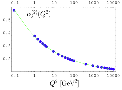
Figure 7: The solid line shows the approximate expression, given by $\bar{\alpha}_{s}^{(2,\text{fit})}(Q^{2})$, Eq. (75), whereas the bullets represent the exact values of $\bar{\alpha}_{s}^{(2)}(Q^{2})$ taking into account heavy-quark threshold matching.

The only feature not yet taken into account in the above approximation is the matching at the quark-flavor thresholds: $M_{4}=1.3$ GeV, $M_{5}=4.3$ GeV, and $M_{6}=170$ GeV (with $M_{1}=M_{2}=M_{3}=0$). However, taking into account this matching, the approximate formula (72) starts to become inaccurate. As a result of the interpolation procedure, we obtain then in this (so-called “global” fit in the Shirkov–Solovtsov terminology Shirkov (2000)—abbreviated by the self-explaining label “fit”) case another approximation:

$$\bar{\alpha}_{s}^{(2,\text{fit})}(Q^{2}) = \frac{4\pi}{b_{0}(N_{f}=3)}\,\bar{a}_{s}\left[\ell\left(\ln\frac{Q^{2}}{\Lambda_{21}^{2}},c_{21}^{\text{fit}}\right)\right]\,,$$ (75)

with the parameters $c_{21}^{\text{fit}}$ and $\Lambda_{21}$ listed in Table 3. The quality of this approximation ensures a deviation less than $1\%$ in the whole $Q^{2}$ interval and is illustrated in Fig. 7.

To fix the parameter $\Lambda_{\text{QCD}}^{N_{f}=3}$, we use Hagiwara et al. (2002)

$$\bar{\alpha}_{s}^{(2)}(m_{Z}^{2})=0.120$$ (76)

that gives us

$$\Lambda_{\text{QCD}}^{N_{f}=3}=400\text{ MeV}\,.$$ (77)

Let us now focus our attention to powers of the analytic coupling function. By performing the analytic continuation of the $k$-th power of function (68) in the complex $Q^{2}$-plane, one determines the corresponding spectral functions $\rho_{k}^{(2)}(\sigma)$, $k=1,2\ldots$:

$$\rho_{k}^{(2)}(t)=\left(\frac{4\pi}{b_{0}c_{1}}\right)^{k}{\textbf{Im}{}}\left(-\frac{1}{1+W_{1}(z(t))}\right)^{k}\,,$$ (78)

which in turn provide the analytic images ${\cal A}_{k}^{(2)}(Q^{2})$ of $\left[\alpha_{s}^{(2)}(Q^{2})\right]^{k}$; viz.,

$${\cal A}_{k}^{(2)}(Q^{2})=\frac{1}{\pi}\int_{0}^{\infty}d\sigma\frac{\rho_{k}^{(2)}(\sigma)}{\sigma+Q^{2}-i\epsilon}\,.$$ (79)

Table 4: Parameters entering Eq. (81) for different values of the QCD scale parameter $\Lambda_{\text{QCD}}^{N_{f}=3}$.

Parameters	$\Lambda_{\text{QCD}}^{N_{f}=3}=350$ MeV	$\Lambda_{\text{QCD}}^{N_{f}=3}=400$ MeV	$\Lambda_{\text{QCD}}^{N_{f}=3}=450$ MeV
$c_{22}^{\text{fit}}$	$-1.549$	$-1.544$	$-1.534$
$\Lambda_{22}$	$29$ MeV	$34.5$ MeV	$41$ MeV
$\ln(\Lambda_{22}^{2}/1~{}{\text{GeV}^{2}})$	$-7.088$	$-6.734$	$-6.399$

These functions obey a more complicated recurrence relation: ($k=1,2\ldots$)

$$\frac{\partial{\cal A}_{k}^{(2)}(Q^{2})}{\partial\ln Q^{2}}=-k\frac{b_{0}}{4\pi}\left[{\cal A}_{k+1}^{(2)}(Q^{2})+\frac{b_{1}}{4\pi b_{0}}{\cal A}_{k+2}^{(2)}(Q^{2})\right]\,\,\,\text{and}\,\,\,{\cal A}_{1}^{(2)}(Q^{2})\equiv\bar{\alpha}_{s}^{(2)}(Q^{2}/\Lambda^{2})\,.\,\,\,$$ (80)

As a result of the interpolation procedure, we obtain in the “global” case the following approximation for $k=2$

$${\cal A}_{2}^{(2,\text{fit})}(Q^{2}) = \left[\frac{4\pi}{b_{0}(N_{f}=3)}\right]^{2}\left\{\frac{1}{L^{2}}-\frac{\exp(L)}{\left[1-\exp(L)\right]^{2}}\right\}_{L=\ell\left[\ln\left(\frac{Q^{2}}{\Lambda_{22}^{2}}\right),c_{22}^{\text{fit}}\right]}\,,$$ (81)

with the parameters $c_{22}^{\text{fit}}$ and $\Lambda_{22}$ being listed in Table 4. The quality of the approximation is high with the deviation restricted to about $1\%$ ($10\%$) for $Q^{2}\geq 1$ GeV² ($Q^{2}\leq 0.1$ GeV²), as illustrated in Fig. 8. One sees from this figure that for $Q^{2}\geq 10$ GeV² the difference between the exact and approximate expression starts to be negligible with the sizable deviation being confined in the region $Q^{2}\leq 1$ GeV².

   

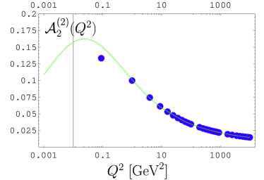
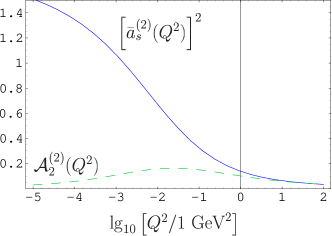
Figure 8: (Left) The solid line represents the approximate expression ${\cal A}_{2}^{(2,\text{fit})}(Q^{2})$ given by Eq. (81), whereas the bullets denote the exact values of ${\cal A}_{2}^{(2)}(Q^{2})$ taking into account the heavy-quark threshold matching. (Right) Comparison of ${\cal A}_{2}^{(2,\text{fit})}(Q^{2})$ (dashed curve) with $[\bar{\alpha}_{s}^{(2,\text{fit})}(Q^{2})]^{2}$ (solid curve). Note the modified scale of the abscissa.

VI.3 Factorization of the pion form factor at NLO under analytization

The analytization procedure of the pion form factor at NLO leads to ambiguities, first discussed in Stefanis et al. (2000). The key question is: according to what analytization prescription are we replacing the running strong coupling and its powers by their analytic images? In fact, it is possible to impose the analytization of the NLO term of $F_{\pi}^{\text{Fact}}$ following two different main options:

• In keeping with our philosophy of the analytization of observables as a whole Karanikas and Stefanis (2001); Stefanis (2003), we may adopt a Maximally Analytic prescription and use in the NLO term of the pion form factor also the analytic image of $\alpha_{s}^{2}$. This amounts to

  $$\!\!\!\!\!\!\left[F_{\pi}^{\text{Fact}}(Q^{2};\mu_{\text{R}}^{2})\right]_{\text{MaxAn}}\ =\ \bar{\alpha}_{s}^{(2)}(\mu_{\text{R}}^{2})\,{\cal F}_{\pi}^{\text{LO}}(Q^{2})+\frac{1}{\pi}\,{\cal A}_{2}^{(2)}(\mu_{\text{R}}^{2})\,{\cal F}_{\pi}^{\text{NLO}}(Q^{2};\mu_{\text{R}}^{2})\,,$$ (82a)

  which will be evaluated with the aid of Eq. (81).

• Another procedure, we call Naive Analytic, replaces the strong coupling and its powers by the analytic coupling $\bar{\alpha}_{s}$ and its powers $\bar{\alpha}_{s}^{2}$ everywhere in the NLO term of $F_{\pi}^{\text{Fact}}$. This is actually the analytization procedure proposed in Stefanis et al. (2000) and amounts to the following requirement

  $$\!\!\!\!\!\!\!\!\!\left[F_{\pi}^{\text{Fact}}(Q^{2};\mu_{\text{R}}^{2})\right]_{\text{NaivAn}}\ =\ \bar{\alpha}_{s}^{(2)}(\mu_{\text{R}}^{2})\,{\cal F}_{\pi}^{\text{LO}}(Q^{2})+\frac{1}{\pi}\,\left[\bar{\alpha}_{s}^{(2)}(\mu_{\text{R}}^{2})\right]^{2}\,{\cal F}_{\pi}^{\text{NLO}}(Q^{2};\mu_{\text{R}}^{2})\,.$$ (82b)

  Note that the naive analytization does not respect nonlinear relations of the coupling owing to different dispersive images.

Anticipating our detailed numerical analysis of the pion form factor using APT, we define

$$\Delta F_{\pi}^{\text{an}}(Q^{2})\equiv\left[F_{\pi}^{\text{Fact}}(Q^{2})\right]_{\text{MaxAn}}-\left[F_{\pi}^{\text{Fact}}(Q^{2})\right]_{\text{NaivAn}}\,,$$ (83)

which provides a quantitative measure for the analytization ambiguity.

VII Pion Form Factor at NLO: Numerical Analysis and Comparison with Experimental Data

In this section we would like to present our predictions for the pion form factor utilizing the BMS pion DA and pQCD at the level of NLO accuracy. First, we consider the standard perturbative approach with different scale settings within the $\overline{\text{MS}\vphantom{{}^{1}}}$ scheme and continue then with a detailed discussion of the pion form factor as a non-power series expansion of the QCD analytic coupling. To this end, we employ the analytization procedures discussed before to obtain $Q^{2}F_{\pi}^{\text{Fact}}$ in the $\overline{\text{MS}\vphantom{{}^{1}}}$ scheme, with different scale settings, and also in the $\alpha_{V}$ scheme. To confront our theoretical predictions with the experimental data in the last subsection, we will include the soft non-factorizable contribution, modelled on the basis of local duality. To join properly the hard and soft contributions, local duality and the Ward identity at $Q^{2}=0$ will be employed in order to ensure that each of these contributions is evaluated in its own region of validity, according to the factorization of the parton and hadron representations. A comparison of these predictions with the corresponding ones obtained with the asymptotic pion DA will be included.

VII.1 Standard perturbative approach

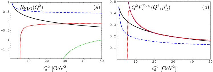
Figure 9: The ratio $R_{\text{NLO}}(Q^{2})$, (a), and the NLO results for $Q^{2}F_{\pi}^{\text{Fact}}$, (b), in the $\overline{\text{MS}}$ scheme with various renormalization scale settings. The dashed line corresponds to $\mu_{\text{R}}^{2}=Q^{2}$, the solid line to the $\overline{\text{BLM}}$ scale setting with $\mu_{\text{min}}^{2}={\mu_{0}^{2}}=1$ GeV², while the dash-dotted one denotes the result obtained with the BLM (a) and FAC (b) scale settings. The analogous result for the PMS scale setting is shown as a dotted line. Note that in both panels the BMS DA has been employed and that for the FAC and PMS scale settings $N_{f}$ has been fixed to 3.

As outlined in Sec. V, the NLO prediction for the pion form factor, as any other finite-order prediction, contains a theoretical uncertainty stemming from its dependence on the renormalization scale $\mu_{\text{R}}$ and the scheme used. This dependence is, however, reduced in comparison with the LO prediction due to the inclusion of the NLO correction. To quantify these statements, we plot in Fig. 9(a) the ratio $R_{\text{NLO}}(Q^{2})=F_{\pi}^{\text{NLO}}(Q^{2})/F_{\pi}^{\text{LO}}(Q^{2})$ and in Fig. 9(b) the result for the factorized form factor at NLO, using the BMS DA in the $\overline{\text{MS}\vphantom{{}^{1}}}$ scheme with different scale settings. The main observation from these figures is the strong sensitivity of $R_{\text{NLO}}(Q^{2})$ and the moderate dependence of $F_{\pi}^{\text{Fact}}(Q^{2})$ on the scale-setting procedure adopted—especially at $Q^{2}$ values accessible to present experiments.

Let us discuss these figures in a systematic way.

• For $\mu_{\text{R}}^{2}=Q^{2}$, the ratio $R_{\text{NLO}}(Q^{2})$ is positive, large (on the order of about $50\%$) and decreases very slowly, while $\alpha_{s}$ is small ($\sim 0.3$). As a result, the LO contribution is about twice as the NLO one and the form factor is small.

• Using the FAC scale setting, the whole NLO contribution vanishes, so that also the ratio is zero. In this case, the form factor is rather moderate down to momenta of the order of $10$ GeV², where the QCD effective coupling becomes of order unity.

• Applying the PMS scale setting, the NLO contribution is negative with $R_{\text{NLO}}(Q^{2})$ being small and also negative down to a critical value of $Q^{2}\simeq 6$ GeV² (see Table 2), where the absolute value of the NLO contribution becomes equal to the LO one and the form factor becomes zero. For this scale setting, already at $Q^{2}\simeq 6$ GeV², the QCD effective coupling starts “feeling” the Landau singularity and becomes excessively large, while above $10$ GeV² the form factor is rather moderate.

• Adopting the BLM procedure, the results are quite similar to those obtained with the PMS scale setting with respect to the ratio $R_{\text{NLO}}(Q^{2})$, whereas the form factor now is negative and very large below $50$ GeV² (lying outside the range of Fig. 9(b)) because the corresponding NLO correction is again negative and even larger. The reason for this behavior is that in this scheme the typical parton virtualities in the Feynman diagrams are much lower than the external scale $Q^{2}$ (see Table 2) giving rise to a large value of the QCD effective coupling.

• The $\overline{\text{BLM}\vphantom{{}^{1}}}$ scale setting has two distinct regimes, characterized by the fact that the ratio $R_{\text{NLO}}(Q^{2})$ changes its sign around $20$ GeV²: in the regime below this momentum value, the result for the form factor resembles that found with the $\mu_{\text{R}}^{2}=Q^{2}$ scale setting, though its fall-off with $Q^{2}$ is not that steep. On the other hand, above $20$ GeV², the form factor almost coincides with the one calculated with the PMS scale setting.

A further complication: it is not clear how to implement quark-mass thresholds when using the FAC and PMS scale settings. Therefore, the predictions shown have been obtained by fixing $N_{f}=3$. This is because both scales depend on $\beta_{0}$ and this induces discontinuities in the form factor at the quark-mass thresholds. For that reason, we refrain from using the FAC and PMS schemes in our further considerations. To summarize, all scale settings can be safely used above about $20$ GeV², while at smaller $Q^{2}$ values, the PMS and FAC settings become unphysical, whereas the $\overline{\text{BLM}\vphantom{{}^{1}}}$ and $\mu_{\text{R}}^{2}=Q^{2}$ scale-setting procedures can further be used at values of $Q^{2}$ exhausting the validity domain of pQCD. On the other hand, the BLM scale setting remains inapplicable up to scales of the order of $50$ GeV² (see Fig. 9a). As already explained before, no predictions in the $\alpha_{V}$ scheme have been shown because this would require the introduction of exogenous IR regulators.

VII.2 Use of non-power series expansions

We turn now to the results obtained in APT. To exploit the effect of the analytization ambiguity on the factorized pion form factor, according to (83), we plot in Fig. 10 (left panel)

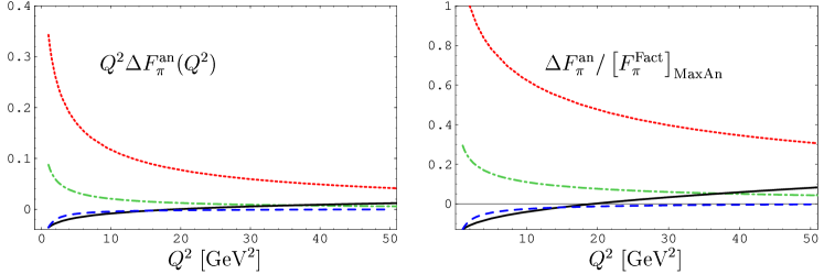
Figure 10: The NLO analytization ambiguity $Q^{2}\Delta F_{\pi}^{\text{an}}(Q^{2})$ (left) and the ratio $\Delta F_{\pi}^{\text{an}}/\left[F_{\pi}^{\text{Fact}}\right]_{\text{MaxAn}}$ of the NLO analytization ambiguity relative to the factorized pion form factor, computed with the “Maximally Analytic” procedure, (right) within the $\overline{\text{MS}}$ scheme with various scale settings: $\mu_{\text{R}}^{2}=Q^{2}$ (dashed line), BLM (dotted line), $\overline{\text{BLM}}$ (solid line), and the $\alpha_{V}$-scheme (dash-dotted line). The curves shown correspond to the BMS DA.

$$\Delta F_{\pi}^{\text{an}}(Q^{2})=\frac{{\cal A}_{2}^{(2)}(\mu_{\text{R}}^{2})-\left[\bar{\alpha}_{s}^{(2)}(\mu_{\text{R}}^{2})\right]^{2}}{\pi}\,{\cal F}_{\pi}^{\text{NLO}}(Q^{2};\mu_{\text{R}}^{2})$$ (84)

and the ratio $\Delta F_{\pi}^{\text{an}}/\left[F_{\pi}^{\text{Fact}}\right]_{\text{MaxAn}}$ (right panel), employing the BMS DA and the $\overline{\text{MS}}$ scheme with different scale settings. Analogous results for the $\alpha_{V}$-scheme are also included; using APT there is no need to introduce external IR regulators.

Summarizing the results in Fig. 10, the main observations are:

• The NLO analytization ambiguity, $\Delta F_{\pi}^{\text{an}}(Q^{2})$, (left panel) and the ratio, $\Delta F_{\pi}^{\text{an}}/F_{\pi}^{\text{Fact}}$, (right panel), the latter being computed with the “Maximally Analytic” procedure within the $\overline{\text{MS}\vphantom{{}^{1}}}$ scheme with the $\mu_{\text{R}}^{2}=Q^{2}$ (dashed line) and $\overline{\text{BLM}\vphantom{{}^{1}}}$ (solid line) scale settings, is small and almost scaling with $Q^{2}$ above about $10$ GeV², albeit in the second case there is a sign change around $18$ GeV². This is because below this momentum, the term $F_{\pi}^{(1,\text{FG})}$, which is negative, prevails, while above that scale the term $F_{\pi}^{(1,\beta)}$ becomes dominant due to $-\ln(Q^{2}/\mu_{\text{R}}^{2})$—in contrast to the former case in which the interplay between these two terms is fixed owing to the absence of the log term. For that reason, the “Maximally Analytic” procedure with the $\overline{\text{BLM}\vphantom{{}^{1}}}$ scale setting enhances the form factor at higher $Q^{2}$ relative to the “Naive” one.

• The results with the BLM scale setting (dotted line) resemble those computed with the $\alpha_{V}$ scheme (dash-dotted line). In both cases, ${\cal A}_{2}^{(2)}(\mu_{\text{R}}^{2})-\left[\bar{\alpha}_{s}^{(2)}(\mu_{\text{R}}^{2})\right]^{2}$ is large and negative (cf. Fig. 8—right panel), while ${\cal F}_{\pi}^{(1,\text{FG})}$ is also negative. Hence, the overall sign of $\Delta F_{\pi}^{\text{an}}(Q^{2})$ is plus because the $F_{\pi}^{(1,\beta)}$ is absent. However, in the $\alpha_{V}$ scheme the shift towards smaller values of the $\alpha_{s}$ argument is much less pronounced and consequently the enhancement provided by the use of ${\cal A}_{2}^{(2)}(\mu_{\text{R}}^{2})$ instead of $\left[\bar{\alpha}_{s}^{(2)}(\mu_{\text{R}}^{2})\right]^{2}$ is rather weak (see also Eq. (LABEL:eq:FpialphaV)).

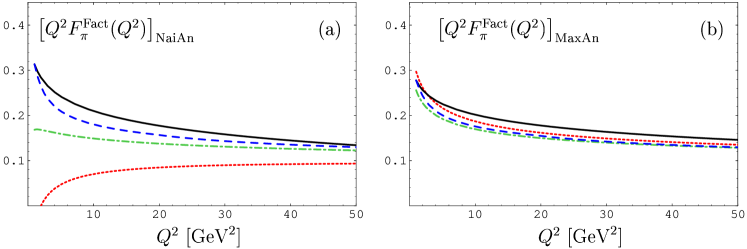
Figure 11: NLO predictions for $Q^{2}F_{\pi}^{\text{Fact}}$ vs. $Q^{2}$, using the “Naive Analytic” (a) and “Maximally Analytic” (b) procedures and employing the BMS DA. The dashed line corresponds to $\mu_{\text{R}}^{2}=Q^{2}$, the dotted one denotes the result obtained with the standard BLM scale setting, whereas the solid line shows the result calculated with the modified $\overline{\text{BLM}}$ scale setting and the cutoff scale ${\mu_{0}^{2}}=1$ GeV². The results obtained with the $\alpha_{V}$-scheme are displayed as a dash-dotted line in both panels.

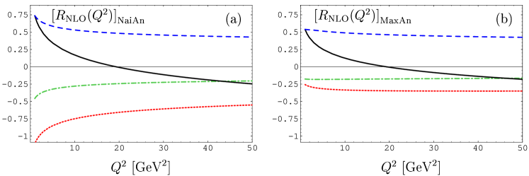
Figure 12: Results obtained for the ratio $R_{\text{NLO}}(Q^{2})$ using the “Naive Analytic” (a) and “Maximally Analytic” (b) procedures and employing the BMS DA. Notations are the same as in figure 11.

Next, we present the results for the factorized pion form factor derived with APT at the NLO level and adopting either the “Naive Analytic” or the “Maximally Analytic” procedure. From Fig. 11, we see that for both analytization procedures the results for the $\mu_{\text{R}}^{2}=Q^{2}$ (dashed line) and $\overline{\text{BLM}}$ (solid line) scale settings are very close to each other. Note that the $\alpha_{V}$-scheme yields a similar result (dash-dotted line), but with a much smaller steepness of the curve at low $Q^{2}$. On the other hand, the standard BLM scale setting (dotted line) produces even an exact cancellation of the NLO and LO terms at the momentum value $Q^{2}\approx 2$ GeV² (so too behaves the ratio $R_{\text{NLO}}(Q^{2})=F_{\pi}^{\text{NLO}}(Q^{2})/F_{\pi}^{\text{LO}}(Q^{2})$—see Fig. 12(a)). The origin of this cancellation is, however, purely accidental and unphysical: the BLM scale at this point is $\mu_{\text{BLM}}^{2}\approx 0.02$ GeV² with $\alpha_{s}\approx 0.75$, rendering the pQCD expansion unreliable. This deficiency is lifted when applying the “Maximally Analytic” procedure—see Fig. 11(b). Indeed, such is the impact of the “Maximally Analytic” condition that all renormalization-scheme and scale-setting ambiguities are diminished, with all results for the form factor almost coinciding, as it is obvious from Fig. 11(b). Moreover, from Fig. 11b, we can estimate the effect of varying $\mu_{\text{min}}^{2}=\mu_{0}^{2}$ in the $\overline{\text{BLM}\vphantom{{}^{1}}}$ scale setting procedure by comparing the $\overline{\text{BLM}\vphantom{{}^{1}}}$ (black solid) and the BLM (red dotted) curves. Indeed, $\mu^{2}_{\text{BLM}}$ just varies from $0.5$ GeV² (at $Q^{2}=50$ GeV²) to $0.02$ GeV² (at $Q^{2}=2$ GeV²), while the difference between these two curves is no more than $10\%$ (using the “Maximally Analytic” condition). Actually, for $\mu^{2}_{\text{min}}$ varying in the range $[1,\;0.5]$ GeV², this difference does not even exceed the level of $5\%$.

Let us close this discussion with some brief comments on the behavior of the ratio $R_{\text{NLO}}(Q^{2})$. The message from Fig. 12 is that, except for the BLM scale setting (already discussed), all other scale-settings are not sensitive to the analytization procedure adopted. The induced differences are indeed marginal, with $R_{\text{NLO}}(Q^{2})$ being positive, large, and practically scaling with $Q^{2}$ for the $\mu_{\text{R}}^{2}=Q^{2}$ scale setting (dashed line), while this quantity in the $\alpha_{V}$ scheme (dash-dotted line) exhibits the same behavior but with the reverse sign and having approximately half of its magnitude. The situation for the $\overline{\text{BLM}\vphantom{{}^{1}}}$ scale setting is somewhat transient between these two options, providing with both analytization procedures enhancement at the low end of $Q^{2}$ and reducing the form factor at $Q^{2}$ values higher than $Q^{2}\simeq 20$ GeV². This effect is due to the (negative) term $F_{\pi}^{(1,\text{FG})}$ gaining ground against $F_{\pi}^{(1,\beta)}$ that becomes smaller because $\ln(Q^{2}/\mu_{\text{R}}^{2})$ is growing.

VII.3 Non-factorizable Contribution to the Pion Form Factor

So far we have discussed only the factorizable part of the pion form factor (cf. (2)). But as argued originally in Refs. Nesterenko and Radyushkin (1982, 1983); Isgur and Llewellyn Smith (1984); Radyushkin (1991), and confirmed latter on in several works, for instance, in Jakob and Kroll (1993); Anisovich et al. (1995); Stefanis et al. (1999); Bakulev et al. (2000); Stefanis et al. (2000), the dominant contribution at low to moderate values of the momentum transfer $Q^{2}\leq 10~{}\text{GeV}^{2}$ originates mainly from the soft contribution that involves no hard-gluon exchanges and is attributed to the Feynman mechanism. At present there is no unique way to calculate this contribution from first principles at the partonic level. One has to resort to theoretical models, based on assumptions that attempt to capture the characteristic features of nonperturbative QCD. In the present investigation we use the Local Duality (LD) approach to calculate the soft contribution, in which it is assumed that the pion form factor is dual to the free quark spectral density Nesterenko and Radyushkin (1982); Radyushkin (1995), i.e.,

$$F_{\pi}^{\text{LD}}(Q^{2}) = \frac{1}{\pi^{2}f_{\pi}^{2}}\int_{0}^{s_{0}}\!\!\!\int_{0}^{s_{0}}\rho_{3}(s,s^{\prime},Q^{2})\ ds\ ds^{\prime}\ =\ 1-\frac{1+6\ s_{0}/Q^{2}}{\left(1+4\ s_{0}/Q^{2}\right)^{3/2}}\,,$$ (85)

with the 3-point spectral density $\rho_{3}(s,s^{\prime},t=Q^{2})$ given by

$$\rho_{3}(s,s^{\prime},t)=\left[t^{2}\frac{d^{2}}{dt^{2}}+\frac{t^{3}}{3}\frac{d^{3}}{dt^{3}}\right]\frac{1}{\lambda\left(s,s^{\prime},t\right)}$$ (86)

where

$$\lambda\left(s,s^{\prime},t\right)\equiv\sqrt{\left(s+s^{\prime}+t\right)^{2}-4ss^{\prime}}\,.$$ (87)

Here the duality interval $s_{0}$ corresponds to the effective threshold for the higher excited states and the “continuum” in the channels with the axial-current quantum numbers. The LD prescription for the corresponding correlator Shifman et al. (1979) implies the relation

$$s_{0}=4\pi^{2}f_{\pi}^{2}\,.$$ (88)

A key issue of the soft contribution is the inclusion of Sudakov-type radiative corrections. In Bakulev et al. (2000) only the Sudakov corrections to the quark-photon vertex were taken into account on the basis of Bakulev (1995) leading to a reduction of the soft contribution by approximately 6% at low $Q^{2}\simeq 2$ GeV² and up to 20% at higher $Q^{2}$ values. Just recently, however, it was shown in Braguta and Onishchenko (2004) that taking into account all radiative corrections to the correlator, the Sudakov logarithms cancel out. On the face of this finding, we use in this work Eqs. (85)–(86).

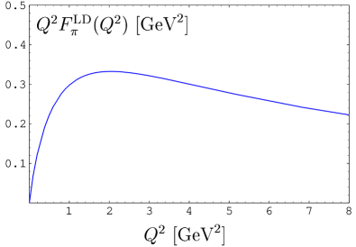
Figure 13: Calculation of the soft part of the pion form factor in the Local Duality approach.

The soft contribution calculated here is consistent with the result obtained in Stefanis et al. (2000) for the asymptotic pion DA on the basis of the soft overlap of the pion wave functions, modelling their $k_{\perp}$ dependence in terms of the Brodsky–Huang–Lepage Gaussian ansatz Brodsky et al. (1983b) and using a constituent-like quark mass of $m_{q}=330$ MeV. Though the crossover from the soft to the hard regime and the asymptotic behavior are strongly model dependent, with the mass factor $\exp\left(-\beta_{\text{G}}^{2}m_{q}^{2}/x\bar{x}\right)$ (where $\beta_{\text{G}}$ is the width of the Gaussian distribution, specific for each particular pion DA) playing an important role in tuning this behavior—see Jakob and Kroll (1993) for a detailed analysis—the trend at lower values of $Q^{2}$ up to about $4$ GeV² is approximately the same. Similar results were also obtained in Kisslinger and Wang (1993) using a Bethe-Salpeter equation and a constituent-type quark mass of $m_{q}=330$ MeV. In both approaches mentioned Stefanis et al. (2000); Kisslinger and Wang (1993) the quark mass in the hard part was set equal to zero and the effective QCD coupling was assumed to saturate at low $Q^{2}$ with a transition scale from soft to hard in the range $Q^{2}\simeq 12-18$ GeV².

VII.4 Comparison with experimental data

It is time to step up one level higher and consider the total form factor in order to compare our theoretical predictions with the experimental data. So far we have considered the factorized hard contribution to the pion form factor only at higher values of $Q^{2}$, where pQCD is safe. However, attempting to compute the total pion form factor in the full $Q^{2}$ range, according to Eq. (2), we have to combine this contribution with the soft part. Recall that we have neglected in the hard-scattering amplitude (i.e., in the parton propagators—cf. Eqs. (102), (107a), and (108)) all parton transverse momenta against the large scale $Q^{2}$ and integrated out in the pion wave functions all transverse momenta up to the scale ${\mu_{0}^{2}}$. But below some momentum scale of this order, these contributions in $T_{\text{H}}$ start to be comparable (especially in the endpoint region where $x\to 1$) and, a fortiori, the collinear factorization becomes increasingly unreliable. To avoid this happening, we have to restrict the evaluation of the hard form-factor contribution to that $Q^{2}$ domain compatible with the collinear approximation. In technical terms this means that below the scale $s_{0}$ (the duality threshold) we have to switch from the parton representation to the hadron representation according to local duality.

As we have seen in Sec. V, fixing the renormalization scale $\mu_{\text{R}}^{2}$ in all considered schemes entails problems related to the small $Q^{2}$-behavior of the factorizable term of the pion form factor: the NLO-term can reach the level of 50% of the LO part, casting doubts on the validity of the perturbative expansion per se. In addition, both terms (LO and NLO) generate a fast growth of the form factor at small $Q^{2}$, artificially induced by large values of the strong coupling and by a $1/Q^{2}$-factor. The origin of this failure, as stated above, can be traced to the violation of the collinear factorization approximation, i.e., the resurrection of small momenta in $T_{\text{H}}$ that have initially been neglected and absorbed into the pion DA.

Hence, it becomes clear that we must correct the factorization results in the low-$Q^{2}$ region in order to ensure that each contribution lies in the corresponding domain of validity. To achieve this goal, we need a conceptual framework.

This is provided by gauge invariance that protects the value of $F_{\pi}(0)$ by means of the Ward identity relating a three-point Feynman diagram at zero-momentum transfer to a 2-point diagram. Consider the $L$-loop approximation in the LD approach. Then, using the replacements $s_{0}\to s_{0}^{L-\text{loop}}$ and $\rho_{3}(s,s^{\prime},Q^{2};\mu_{\text{R}}^{2})\to\rho_{3}^{L-\text{loop}}(s,s^{\prime},Q^{2};\mu_{\text{R}}^{2})$, Eq. (85) relates $F_{\pi}^{\text{LD}}(Q^{2})$ to the integrated 3-point spectral density $\rho_{3}^{L-\text{loop}}(s,s^{\prime},Q^{2};\mu_{\text{R}}^{2})$, which is now dependent on $\mu_{\text{R}}^{2}$. Recall that the Ward identity links the 2-point (i.e., axial-axial current) spectral density $\rho_{2}^{L-\text{loop}}(s;\mu_{\text{R}}^{2})$ to the 3-point (vector-axial-axial current) spectral density $\rho_{3}^{L-\text{loop}}(s,s^{\prime},0;\mu_{\text{R}}^{2})$ in the following way

$$\rho_{3}^{L-\text{loop}}(s,s^{\prime},0;\mu_{\text{R}}^{2}) = \pi\delta(s-s^{\prime})\rho_{2}^{L-\text{loop}}(s;\mu_{\text{R}}^{2})\,.$$ (89)

Taking into account the LD expression for the pion decay constant,

$$f_{\pi}^{2} = \frac{1}{\pi}\int_{0}^{s_{0}^{L\text{-loop}}}\rho_{2}^{L\text{-loop}}(s;\mu_{\text{R}}^{2})\ ds\,,$$ (90)

one finds

$$F_{\pi}^{\text{LD}}(0;\mu_{\text{R}}^{2}) = 1\,.$$ (91)

The 2-loop approximation for the spectral density, $\rho_{2}^{\text{2-loop}}(s;\mu_{\text{R}}^{2})$, can be obtained from the $e^{+}e^{-}$ cross-section $R(s)$ Chetyrkin et al. (1979), because these quantities in massless QCD are proportional to each other, so that

$$\rho_{2}^{\text{2-loop}}(s;\mu_{\text{R}}^{2}) = \frac{1}{4\pi}\left[1+\frac{\alpha_{s}(\mu_{\text{R}}^{2})}{\pi}+\left(\frac{\alpha_{s}(\mu_{\text{R}}^{2})}{\pi}\right)^{2}\left(r_{2}-\frac{b_{0}}{4}\ln\frac{s}{\mu_{\text{R}}^{2}}\right)\right]\,;$$ (92)

$$r_{2} = \frac{3}{4}\,C_{\text{F}}\left[\frac{1}{12}\,C_{\text{A}}-\frac{1}{8}\,C_{\text{F}}+b_{0}\left(\frac{11}{8}-\zeta(3)\right)\right]\,,$$ (93)

where $\zeta(3)$ is the Riemann Zeta function. Then, Eq. (90) yields the following nonlinear relation for the 2-loop effective threshold $s_{0}^{\text{2-loop}}$

$$s_{0}^{\text{2-loop}}\left\{1+\frac{\alpha_{s}(\mu_{\text{R}}^{2})}{\pi}+\left(\frac{\alpha_{s}(\mu_{\text{R}}^{2})}{\pi}\right)^{2}\left[r_{2}-\frac{b_{0}}{4}\left(\ln\frac{s_{0}^{\text{2-loop}}}{\mu_{\text{R}}^{2}}-1\right)\right]\right\} = 4\pi^{2}f_{\pi}^{2}$$ (94)

that replaces the standard LD relation, notably, Eq. (88). Note in this context that the effective 2-loop threshold $s_{0}^{\text{2-loop}}$ should be used only in formulas containing the 2-loop spectral density $\rho_{3}^{\text{2-loop}}(s,s^{\prime},Q^{2})$. Were we in the position to write down the 2-loop spectral density $\rho_{3}^{\text{2-loop}}(s,s^{\prime},Q^{2})$ for all $Q^{2}$ values, then we would have obtained via Eqs. (85)-(90) an expression for the pion form factor valid at $O(\alpha_{s}^{2})$. Instead, we use the leading-order LD expression, $F_{\pi}^{\text{LD}}(Q^{2};\mu_{\text{R}}^{2})$, and add perturbative $O(\alpha_{s})$- and $O(\alpha_{s}^{2})$-corrections explicitly in terms of $F_{\pi}^{\text{Fact}}(Q^{2};\mu_{\text{R}}^{2})$. Recalling Eq. (91), we then have

$$F_{\pi}^{\text{Fact}}(Q^{2}=0;\mu_{\text{R}}^{2})=0\,.$$ (95)

The next task is to match this low-$Q^{2}$ value with the large-$Q^{2}$ result of pQCD, $F_{\pi}^{\text{Fact}}(Q^{2};\mu_{\text{R}}^{2})$. The most straightforward way is to adopt $F_{\pi}^{\text{Fact}}(Q^{2};\mu_{\text{R}}^{2})$ at large $Q^{2}$ and correct its singular ($\sim 1/Q^{2}$) behavior at small $Q^{2}$ by introducing some reasonable mass scale $M_{0}^{-1}$ via the replacement

$$F_{\pi}^{\text{Fact}}(Q^{2};\mu_{\text{R}}^{2}) \equiv \tilde{F}_{\pi}(Q^{2};\mu_{\text{R}}^{2})\frac{M_{0}^{2}}{Q^{2}}\ \to\ \tilde{F}_{\pi}(Q^{2};\mu_{\text{R}}^{2})\frac{M_{0}^{2}}{M_{0}^{2}+Q^{2}}\,.$$ (96)

However, this expression has the wrong limit at $Q^{2}=0$, so that one needs to correct it in order to maintain the Ward identity (WI):

$$F_{\pi}^{\text{Fact-WI}}(Q^{2};\mu_{\text{R}}^{2}) = -\tilde{F}_{\pi}(Q^{2};\mu_{\text{R}}^{2})\,\Phi(Q^{2}/M_{0}^{2})+\tilde{F}_{\pi}(Q^{2};\mu_{\text{R}}^{2})\frac{M_{0}^{2}}{M_{0}^{2}+Q^{2}}\,.$$ (97)

Here the function $\Phi(z)$ is some smooth function with $\Phi(0)=1$ and $z\Phi(z)\to 0$ when $z\to\infty$, introduced to preserve the high $Q^{2}$-asymptotics of $F_{\pi}^{\text{Fact}}(Q^{2};\mu_{\text{R}}^{2})$. The simplest choice for $\Phi(z)$ is $\Phi(z)=1/(1+z)^{2}$, yielding

$$F_{\pi}^{\text{Fact-WI}}(Q^{2};\mu_{\text{R}}^{2}) = \tilde{F}_{\pi}(Q^{2};\mu_{\text{R}}^{2})\frac{M_{0}^{2}}{M_{0}^{2}+Q^{2}}\left(1-\frac{M_{0}^{2}}{M_{0}^{2}+Q^{2}}\right)$$ (98)

$$= F_{\pi}^{\text{Fact}}(Q^{2};\mu_{\text{R}}^{2})\left(\frac{Q^{2}}{M_{0}^{2}+Q^{2}}\right)^{2}\,.$$

The scale parameter $M_{0}^{2}$ should be identified with the threshold $2s_{0}^{\text{2-loop}}$ to read $M_{0}^{2}=2s_{0}^{\text{2-loop}}$ because $s_{0}^{\text{2-loop}}$ is the “natural” scale parameter for the 2-point correlator in the pion case, while the scale characterizing the 3-point correlator, corresponding to the form factor, is two times larger Bakulev and Radyushkin (1991).

In this way, we finally arrive at

$$F_{\pi}^{\text{Fact-WI}}(Q^{2};\mu_{\text{R}}^{2}) = \left(\frac{Q^{2}}{2s_{0}^{\text{2-loop}}+Q^{2}}\right)^{2}F_{\pi}^{\text{Fact}}(Q^{2};\mu_{\text{R}}^{2})\,.$$ (99)

We are now in the position to supply an expression for the total pion form factor valid in the whole $Q^{2}$ range:

$$F_{\pi}(Q^{2};\mu_{\text{R}}^{2})=F_{\pi}^{\text{LD}}(Q^{2})+F_{\pi}^{\text{Fact-WI}}(Q^{2};\mu_{\text{R}}^{2})\,.$$ (100)

This expression comprises the NLO prediction for the factorized part under the proviso of the Ward identity at $Q^{2}=0$ and the non-factorizable soft part. [Parenthetically, note the explicit $\mu_{\text{R}}^{2}$ dependence of this expression as a consequence of the truncation of the perturbative series (see Eqs. (23)–(30)).]

Before continuing with the presentation of our final results, let us remark that a similar type of matching has been applied by Radyushkin Radyushkin (1995) to describe the pion form factor, providing the result

$$F_{\pi}(Q^{2})=\frac{F_{\pi}^{\text{LD(0)}}(Q^{2})+\left(\alpha_{s}/\pi\right)\left[1+Q^{2}/\left(2s_{0}\right)\right]^{-1}}{1+\alpha_{s}/\pi}$$ (101)

illustrated in Fig. 14 (a) (dash-dotted line).

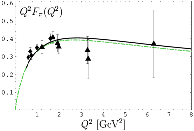
Figure 14: Comparison of the pion form factor calculated by Radyushkin Radyushkin (1995) using the LD approach and interpolation from low to high $Q^{2}$ (dash-dotted line) with our result for the total form factor given by Eq. (100), computed with the asymptotic DA in the $\overline{\text{MS}\vphantom{{}^{1}}}$ scheme with the $\overline{\text{BLM}\vphantom{{}^{1}}}$ scale setting and using LO APT (solid line). The experimental data are taken from Volmer et al. (2001) (diamonds) and Brown et al. (1973), Bebek et al. (1976) (triangles).

In this equation—which follows the Brodsky–Lepage interpolation formula for the $\pi\gamma$-transition form factor Brodsky and Lepage (1980)—the first term means the soft form factor calculated with the LD approach, while the second one includes the LO radiative corrections. It is evident from this figure that Radyushkin’s result is very close to that given by Eq. (100), evaluated with the asymptotic DA in the $\overline{\text{MS}\vphantom{{}^{1}}}$ scheme with the $\overline{\text{BLM}\vphantom{{}^{1}}}$ scale setting using for the sake of comparison LO APT (solid line).

Employing the above considerations we now present predictions for the total scaled form factor vs. $Q^{2}$ in different renormalization schemes and perturbation-theory approaches using the BMS pion DA. Figure 15 shows the results for the standard perturbation theory within the $\overline{\text{MS}\vphantom{{}^{1}}}$ scheme adopting the $\mu_{\text{R}}^{2}=Q^{2}$ (dashed line) and the $\overline{\text{BLM}\vphantom{{}^{1}}}$ (solid line) scale settings. In Fig. 16 we present analogous predictions calculated with the APT. In this case, it is possible to include results computed with the BLM scale setting and to use the $\alpha_{V}$ scheme. We observe from this figure (left panel) that the “Naive Analytization” gives results that bear a rather strong scheme and scale-setting dependence. In contrast, applying the “Maximal Analytic” procedure, the arbitrariness in the scheme and scale setting is minimized—Fig. 16(b) being a graphic proof of that. Note that this figure shows also separately the soft part of the form factor, displayed in Fig. 13, and the hard contributions corresponding to the various scheme and scale settings discussed above and presented in Fig. 11(b).

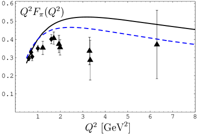
Figure 15: Theoretical predictions for $Q^{2}F_{\pi}(Q^{2})$ obtained with the BMS pion DA using standard pQCD within the $\overline{\text{MS}}$ scheme and adopting the $\mu_{\text{R}}^{2}=Q^{2}$ (dashed line) and $\overline{\text{BLM}}$ (solid line) scale settings. The experimental data are taken from Volmer et al. (2001) (diamonds) and Brown et al. (1973), Bebek et al. (1976) (triangles).

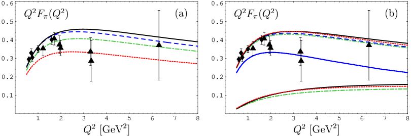
Figure 16: Theoretical predictions for $Q^{2}F_{\pi}(Q^{2})$ using analytic perturbation theory and the BMS DA in conjunction with the “Naive Analytic” (a) and “Maximally Analytic” (b) analytization procedures. Different scale settings within the $\overline{\text{MS}}$ scheme are used: $\mu_{\text{R}}^{2}=Q^{2}$ (dashed line), BLM (dotted line), and $\overline{\text{BLM}}$ (solid line). The dash-dotted line represents the prediction obtained with the $\alpha_{V}$-scheme. Also included are the prediction for the soft form-factor part (solid blue line) and below this, the hard contributions in correspondence with the predictions for the total form factor on the upper part of the figure. The experimental data are taken from Volmer et al. (2001) (diamonds) and Brown et al. (1973), Bebek et al. (1976) (triangles).

The phenomenological upshot of our analysis is summarized in the left panel of Fig. 17, where we show predictions for the whole BMS “bunch” of pion DAs Bakulev et al. (2001). The shaded strip incorporates the nonperturbative uncertainties related to non local QCD sum rules and also the ambiguities induced by the scheme and renormalization scale setting—in correspondence to Fig. 16. Note that the two broken lines mark the region of predictions associated with the asymptotic pion DA. These results can be compared with previous theoretical predictions and also with further experimental data to be obtained at JLab (see right part of Fig. 17, taken from Blok et al. (2002)). The data points extending to $Q^{2}$ of $6$ GeV² are expectations from projected experiments at JLab after the planned upgrade of CEBAF to 12 GeV (we refer to Blok et al. (2002) for further explanations and related references).

These striking findings give convincing evidence that the end-point suppressed structure of the BMS type pion DA not only provides best agreement with the CLEO and CELLO data (cf. Fig. 4), it also allows to describe the pion form-factor data with at least the same quality as with the asymptotic pion DA—as it becomes evident from the LHS of Fig. 17.

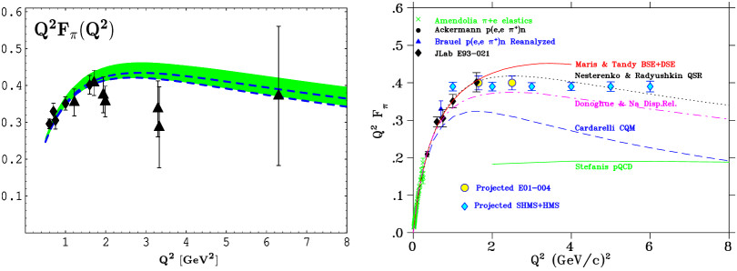
Figure 17: (Left) Predictions for the scaled pion form factor calculated with the BMS bunch (green strip) encompassing nonperturbative uncertainties from nonlocal QCD sum rules Bakulev et al. (2001) and renormalization scheme and scale ambiguities at the level of the NLO accuracy, as discussed in Fig. 16. The dashed lines inside the strip indicate the corresponding area of predictions obtained with the asymptotic pion DA. Note that this strip contains only perturbative scheme and scale ambiguities at the level of the NLO accuracy, calculated in APT with the “Maximally Analytic” procedure. The experimental data are taken from Volmer et al. (2001) (diamonds) and Brown et al. (1973), Bebek et al. (1976) (triangles). (Right) Summary of existing and projected experimental data on the electromagnetic pion form factor in comparison with the results of various theoretical calculations; figure taken from Blok et al. (2002) (see there for explanations).

VIII Summary and conclusions

In summary, the key concepts and merits arising from this analysis are as follows.

• We worked out interpolation formulas for the analytic coupling constant and its analytic second power that take into account heavy-flavor thresholds and greatly facilitate calculations. This allowed us to develop a theoretical procedure and apply its numerical realization in order to compute the evolution of the pion DA using NLO analytic perturbation theory. The hard form factor was corrected at low $Q^{2}$ as to fulfill the Ward identity and was added to the soft form factor, derived via Local Duality, without introducing double counting.

• On the theoretical front, we found that replacing the QCD effective coupling and its powers by their analytic images—a procedure we termed “Maximally Analytic”—not only provides IR protection to the coupling, it also helps diminishing the renormalization scheme and scale-setting dependence of the form-factor predictions already at the NLO level, rendering the calculation of still higher-order corrections virtually superfluous.

• From the phenomenological point of view, our most discernible result is that the BMS pion DA Bakulev et al. (2001) (out of a “bunch” of similar doubly-peaked endpoint-suppressed pion DAs) yields to predictions for the electromagnetic form factor very close to those obtained with the asymptotic pion DA. Hence, concerns that a double-humped pion DA could jeopardize the sound application of pQCD are unduly. Conversely, we have shown that a small deviation of the prediction for the pion form factor from that obtained with the asymptotic pion DA does not necessarily imply that the underlying pion DA has to be close to the asymptotic profile. Much more important is the behavior of the pion DA in the endpoint region $x\to 0\,,1$.

Looking further into the future is yet more exciting. With the planned upgrade of the CEBAF experiment to 12 GeV, the pion’s electromagnetic form factor can be studied up to $Q^{2}\simeq 6$ GeV² Blok et al. (2002), providing crucial constraints to verify the various theoretical predictions discussed here and elsewhere. The apparently good agreement of our results with the available experimental data (see Fig. 17) is encouraging.

Appendix A Hard-scattering amplitude for the pion’s electromagnetic form factor at NLO

In this section we list the NLO results for the hard-scattering amplitude Field et al. (1981); Dittes and Radyushkin (1981); Sarmadi (1983); Radyushkin and Khalmuradov (1985); Kadantseva et al. (1986); Braaten and Tse (1987); Melić et al. (1999), used in our analysis.

The LO contribution to $T_{\text{H}}(x,y,Q^{2};\mu_{\text{F}}^{2})$, expanded as in (4), reads

$$T_{\text{H}}^{(0)}(x,y,Q^{2})=\frac{N_{\text{T}}}{Q^{2}}\,\frac{1}{\overline{x}\,\overline{y}\,}\,,$$ (102)

where

$$N_{\text{T}}=\frac{2\,\pi\,C_{\text{F}}}{C_{\text{A}}}=\frac{8\pi}{9}\,,$$ (103)

$C_{\text{F}}=\left(N_{\rm c}^{2}-1\right)/2N_{\rm c}=4/3$, $C_{\text{A}}=N_{\rm c}=3$ are the color factors of $SU(3)_{\rm c}$, and the notation $\bar{z}\equiv 1-z$ has been used. The usual color decomposition of the NLO correction—marked by self-explainable labels—is given by

$$T_{\text{H}}^{(1)}\left(Q^{2};\mu_{\text{F}}^{2},\mu_{\text{R}}^{2}\right)=C_{\text{F}}\,T_{\text{H}}^{(1,\text{F})}\left(Q^{2};\mu_{\text{F}}^{2}\right)+b_{0}\,T_{\text{H}}^{(1,\beta)}\left(Q^{2};\mu_{\text{R}}^{2}\right)+C_{\text{G}}\,T_{\text{H}}^{(1,\text{G})}\left(Q^{2}\right)\,,$$ (104)

where $C_{\text{G}}=(C_{\text{F}}-C_{\text{A}}/2)$ and the first coefficients of the $\beta$ function are

$$b_{0}=\frac{11}{3}C_{\text{A}}-\frac{4}{3}T_{\text{R}}N_{f}\,,\qquad\qquad b_{1}=\frac{34}{3}C_{\text{A}}^{2}-\left(4C_{\text{F}}+\frac{20}{3}C_{\text{A}}\right)T_{\text{R}}N_{f}\,.$$ (105)

Here, $T_{\text{R}}=1/2$ and $N_{f}$ denotes the number of flavors, whereas the expansion of the $\beta$-function in the NLO approximation is given by

$$\beta(\alpha_{s}(\mu^{2}))=-\alpha_{s}(\mu^{2})\left\{b_{0}\left[\frac{\alpha_{s}(\mu^{2})}{4\pi}\right]+b_{1}\left[\frac{\alpha_{s}(\mu^{2})}{4\pi}\right]^{2}\right\}\,.$$ (106)

With reference to the application of the BLM Brodsky et al. (1983a) scale setting in fixing the renormalization point, we single out the $b_{0}$-proportional (i.e., $N_{f}$-dependent) term, given by

$$T_{\text{H}}^{(1,\beta)}\left(x,y,Q^{2};\mu_{\text{R}}^{2}\right) = \frac{N_{\text{T}}}{Q^{2}}\,\frac{1}{\overline{x}\,\overline{y}\,}\,\left[\frac{5}{3}-\ln(\overline{x}\,\overline{y}\,)-\ln\frac{Q^{2}}{\mu_{\text{R}}^{2}}\right]\,,$$ (107a)

and present the remainder of $$T_{\text{H}}$$ as a color decomposition in the form

$$T_{\text{H}}^{(1,\text{F})}(x,y,Q^{2};\mu_{\text{F}}^{2}) = \frac{N_{\text{T}}}{Q^{2}}\,\frac{1}{\overline{x}\,\overline{y}\,}\,\left[-\frac{28}{3}+\left(6-\frac{1}{x}\right)\ln\overline{x}\,+\left(6-\frac{1}{y}\right)\ln\overline{y}\,+\ln^{2}(\overline{x}\,\overline{y}\,)\right.$$ (107b)

$$\left.+2\ln\frac{Q^{2}}{\mu_{\text{F}}^{2}}\left(3+\ln(\overline{x}\,\overline{y}\,)\right)\right]$$

$$T_{\text{H}}^{(1,\text{G})}(x,y,Q^{2}) = \frac{N_{\text{T}}}{Q^{2}}\,\frac{1}{\overline{x}\,\overline{y}\,}\,\left[-\frac{20}{3}-8\frac{\ln\overline{x}\,}{x}-8\frac{\ln\overline{y}\,}{y}-2\ln\overline{x}\,\ln\overline{y}\,-2\ln x\ln y\right.$$

$$\left.+2\ln x\ln\overline{y}\,+2\ln\overline{x}\,\ln y-2(1-x-y)\text{H}(x,y)-2\,\text{R}(x,y)\right]$$

for the color singlet and color non-singlet parts, respectively. For calculational convenience, we also supply the sum of these terms (cf. Eq. (LABEL:eq:Q2pff1FG)):

$$T_{\text{H}}^{(1,\text{FG})}\left(x,y,Q^{2};\mu_{\text{F}}^{2}\right) = C_{\text{F}}\,T_{\text{H}}^{(1,\text{F})}\left(x,y,Q^{2};\mu_{\text{F}}^{2}\right)+C_{\text{G}}\,T_{\text{H}}^{(1,\text{G})}\left(x,y,Q^{2}\right)$$ (108)

$$= \frac{N_{\text{T}}}{Q^{2}}\,\frac{1}{\overline{x}\,\overline{y}\,}\,\frac{1}{3}\,\Biggl{\{}-34+24\ln(\overline{x}\,\overline{y}\,)+4\ln^{2}(\overline{x}\,\overline{y}\,)$$

$$+\ln x\ln y+\ln\overline{x}\,\ln\overline{y}\,-\ln x\ln\overline{y}\,-\ln\overline{x}\,\ln y$$

$$+(1-x-y)\text{H}(x,y)+\text{R}(x,y)+8\,\left[3+\ln(\overline{x}\,\overline{y}\,)\right]\,\ln\frac{Q^{2}}{\mu_{\text{F}}^{2}}\Biggr{\}}\,,$$

where

$$\text{H}(x,y) = \frac{1}{1-x-y}\left[{\textbf{Li}_{2}}\left(\frac{\overline{y}\,}{x}\right)+{\textbf{Li}_{2}}\left(\frac{\overline{x}\,}{y}\right)+{\textbf{Li}_{2}}\left(\frac{xy}{\overline{x}\,\overline{y}\,}\right)\right.$$ (109a)

$$\left.\qquad\qquad\ -{\textbf{Li}_{2}}\left(\frac{x}{\overline{y}\,}\right)-{\textbf{Li}_{2}}\left(\frac{y}{\overline{x}\,}\right)-{\textbf{Li}_{2}}\left(\frac{\overline{x}\,\overline{y}\,}{xy}\right)\right]$$

with $${\textbf{Li}_{2}} {\textbf{Li}_{2}}(z)=-\int_{0}^{z}\frac{\ln(1-t)dt}{t}$$ being the di-logarithm function, defined by , and

$$\text{R}(x,y) = \frac{1}{(x-y)^{2}}\Bigl{[}(2xy-x-y)(\ln x+\ln y)$$ (109b)

$$+(-2xy^{2}-2y^{2}+10xy-2y-4x^{2})\frac{\ln\overline{y}\,}{y}$$

$$+(-2yx^{2}-2x^{2}+10xy-2x-4y^{2})\frac{\ln\overline{x}\,}{x}$$

$$-(y\overline{y}\,^{2}+x\overline{x}\,^{2})\text{H}(x,\overline{y}\,)\Bigr{]}\,.$$

Appendix B Factorization scale dependence in standard pQCD

Here we examine the $\mu_{\text{F}}^{2}$-dependence of the hard-scattering amplitude (see, for example, Lepage and Brodsky (1979); Efremov and Radyushkin (1980a); Melić et al. (2002, 2001); Passek (2001)). We start with the representation for $T_{H}(\mu_{\text{F}}^{2},\mu_{\text{R}}^{2})$, given by (4), to get

$$T_{\text{H}}(\mu_{\text{F}}^{2},\mu_{\text{R}}^{2}) = \alpha_{s}(\mu_{R}^{2})\left[T_{\text{H}}^{(0)}+\frac{\alpha_{s}(\mu_{R}^{2})}{4\pi}T_{\text{H}}^{(1)}(\mu_{\text{F}}^{2},\mu_{\text{R}}^{2})\right]$$ (110)

with $T_{\text{H}}^{(0)}(x,y,Q^{2})$ and $T_{\text{H}}^{(1)}(x,y,Q^{2};\mu_{\text{F}}^{2},\mu_{\text{R}}^{2})$ as in (102) and (104) for the LO and NLO, respectively. These functions can be represented as follows

$$T_{\text{H}}^{(0)} = N_{\text{T}}C_{0}(x,y,Q^{2})\,,\quad\text{and~{}~{}~{}}C_{0}=\frac{1}{\bar{x}\bar{y}Q^{2}}\,,$$ (111)

$$T_{\text{H}}^{(1)}(\mu_{\text{F}}^{2},\mu_{\text{R}}^{2}) = \ln\left(\frac{Q^{2}}{\mu_{\text{F}}^{2}}\right)\left[T_{\text{H}}^{(0)}(x,s,Q^{2})\mathop{\otimes}\limits_{s}V_{0}(s,y)+V_{0}(s,x)\mathop{\otimes}\limits_{s}T_{\text{H}}^{(0)}(s,y,Q^{2})\right]$$ (112)

$$- b_{0}\ln\left(\frac{Q^{2}}{\mu_{\text{R}}^{2}}\right)T_{\text{H}}^{(0)}(x,y,Q^{2})+N_{\text{T}}C_{1}(x,y,Q^{2})\,,$$

where $C_{1}(x,y,Q^{2})$ absorbs all other $\mu_{\text{F}}^{2}$- and $\mu_{\text{R}}^{2}$-independent terms from (104). Using this structure with respect to the $\mu_{\text{F}}^{2}$-dependence, we can conclude that

$$\frac{dT_{H}}{d\ln\mu_{\text{F}}^{2}} = -T_{H}(\mu_{\text{F}}^{2},\mu_{\text{R}}^{2})\mathop{\otimes}\limits V(\alpha_{s}(\mu_{\text{R}}^{2}))-V(\alpha_{s}(\mu_{\text{R}}^{2}))\mathop{\otimes}\limits T_{H}(\mu_{\text{F}}^{2},\mu_{\text{R}}^{2})+O(\alpha_{s}^{3})\,,$$ (113)

where $V(\alpha_{s}(\mu_{\text{R}}^{2}))$ is the ERBL evolution kernel (119). Then, the whole derivative of the form factor (3) is

$$\frac{dF_{\pi}(Q^{2};\mu_{\text{R}}^{2})}{d\ln\mu_{\text{F}}^{2}} = \Phi_{\pi}(\mu_{\text{F}}^{2})\mathop{\otimes}\limits T_{H}(\mu_{\text{F}}^{2},\mu_{\text{R}}^{2})\mathop{\otimes}\limits\left[V(\alpha_{s}(\mu_{\text{F}}^{2}))-V(\alpha_{s}(\mu_{\text{R}}^{2}))\right]\mathop{\otimes}\limits\Phi_{\pi}(\mu_{\text{F}}^{2})$$ (114)

$$+ \Phi_{\pi}(\mu_{\text{F}}^{2})\mathop{\otimes}\limits\left[V(\alpha_{s}(\mu_{\text{F}}^{2}))-V(\alpha_{s}(\mu_{\text{R}}^{2}))\right]\mathop{\otimes}\limits T_{H}(\mu_{\text{F}}^{2},\mu_{\text{R}}^{2})\mathop{\otimes}\limits\Phi_{\pi}(\mu_{\text{F}}^{2})$$

$$+ O(\alpha_{s}^{3})\,.$$

Recalling that in the 2-loop approximation of the standard pQCD

$$\frac{d\alpha_{s}(\mu^{2})}{d\ln\mu^{2}} = -4\pi b_{0}\left[\frac{\alpha_{s}(\mu^{2})}{4\pi}\right]^{2}\left[1+O(\alpha_{s}(\mu^{2}))\right],$$ (115)

we have

$$V\left(\alpha_{s}(\mu_{\text{F}}^{2})\right)-V\left(\alpha_{s}(\mu_{\text{R}}^{2})\right) = \left[\frac{\alpha_{s}(\mu_{\text{F}}^{2})-\alpha_{s}(\mu_{\text{R}}^{2})}{4\pi}\right]V_{0}+O(\alpha_{s}^{2})\ =\ O(\alpha_{s}^{2})\,,$$ (116)

so that

$$\frac{dF_{\pi}(Q^{2};\mu_{\text{R}}^{2})}{d\ln\mu_{\text{F}}^{2}} = O(\alpha_{s}^{3})\,.$$ (117)

Hence, we conclude that at the level of the NLO approximation of the standard pQCD, the violation of the factorization-scale independence is one order of $\alpha_{s}$ higher.

Appendix C Two-loop evolution of the pion distribution amplitude in standard pQCD

The pion distribution amplitude $\varphi_{\pi}(x,\mu_{\text{F}}^{2})$ satisfies an evolution equation of the form

$$\frac{d\,\varphi_{\pi}(x,\mu_{\text{F}}^{2})}{d\ln\mu_{\text{F}}^{2}}=V(x,u,\alpha_{s}(\mu_{\text{F}}^{2}))\mathop{\otimes}\limits_{u}\varphi_{\pi}(u,\mu_{\text{F}}^{2})\,,$$ (118)

where $V(x,u,\alpha_{s}(\mu_{\text{F}}^{2}))$ is the perturbatively calculable NLO evolution kernel

$$V(x,u,\alpha_{s})=\frac{\alpha_{s}}{4\pi}\,V_{0}(x,u)+\frac{\alpha_{s}^{2}}{(4\pi)^{2}}V_{1}(x,u)\,.$$ (119)

If the distribution amplitude $\varphi_{\pi}(x,{\mu_{0}^{2}})$ is determined at an initial momentum scale ${\mu_{0}^{2}}$ (using some nonperturbative methods), then the integro-differential evolution equation (118) can be integrated using the moment method to give $\varphi_{\pi}(x,\mu_{\text{F}}^{2})$ at any momentum scale $\mu_{\text{F}}^{2}$. The one-Lepage and Brodsky (1980) and two-loop Dittes and Radyushkin (1984); Sarmadi (1984); Mikhailov and Radyushkin (1985) corrections to the evolution kernel were determined in the $\overline{\text{MS}\vphantom{{}^{1}}}$ -scheme, but because of the complicated structure of the two-loop corrections, only the numerical evaluation of the (first few) moments of the evolution kernel was possible Katz (1985); Mikhailov and Radyushkin (1986b). However, making use of conformal-symmetry constraints, the complete analytical form of the NLO solution of the evolution equation (118) has been obtained Müller (1994, 1995). We note that for $\mu_{\text{F}}^{2}\to\infty$ the solution of Eq. (118) takes the asymptotic form $\varphi_{\pi}(x,\mu_{\text{F}}^{2}\to\infty)\equiv\varphi_{\text{as}}(x)=6x(1-x)$.

The pion DA can be cast in the form

$$\varphi_{\pi}(x,\mu_{\text{F}}^{2})=U(x,s;\mu_{\text{F}}^{2},{\mu_{0}^{2}})\mathop{\otimes}\limits_{s}\varphi_{\pi}(s,{\mu_{0}^{2}})\,,$$ (120)

where the operator $U(x,s;\mu_{\text{F}}^{2},{\mu_{0}^{2}})$ describes the evolution from the scale ${\mu_{0}^{2}}$ to the scale $\mu_{\text{F}}^{2}$ and represents the solution of an evolution equation equivalent to (118), given by

$$\frac{d}{d\ln\mu_{\text{F}}^{2}}\,U(x,s;\mu_{\text{F}}^{2},{\mu_{0}^{2}})=V(x,u,\alpha_{s}(\mu_{\text{F}}^{2}))\mathop{\otimes}\limits_{u}U(u,s;\mu_{\text{F}}^{2},{\mu_{0}^{2}})\,.$$ (121)

It is convenient to express the nonperturbative input DA, $\varphi_{\pi}(x,{\mu_{0}^{2}})$, as an expansion over Gegenbauer polynomials $C_{k}^{3/2}(2x-1)$ which represent the eigenfunctions of the LO kernel $V_{0}$, i.e.,

$$\varphi_{\pi}(x,\mu_{0}^{2})=6x(1-x)\left[1+\sum_{m=2}^{\infty}{}^{\prime}a_{m}({\mu_{0}^{2}})\,C_{m}^{3/2}(2x-1)\right]\,,$$ (122)

in which ${\sum}^{\prime}$ denotes the sum over even indices only. The nonperturbative input is now contained in the $a_{m}({\mu_{0}^{2}})$ coefficients. The Gegenbauer polynomials $C_{n}^{3/2}(2x-1)$ satisfy the orthogonalization condition

$$\int_{0}^{1}dx\,x(1-x)\,C_{n}^{3/2}(2x-1)\,C_{m}^{3/2}(2x-1)=N_{n}\,\delta_{nm}$$ (123)

with respect to the weight $x(1-x)$, where

$$N_{n}=\frac{(n+1)(n+2)}{4(2n+3)}\,.$$ (124)

The moments of the evolution kernel

$$M_{kn}\left[\alpha_{s}(\mu_{\text{F}}^{2})\right] = C_{k}^{3/2}(2x-1)\mathop{\otimes}\limits_{x}V\left(x,y;\alpha_{s}(\mu_{\text{F}}^{2})\right)\mathop{\otimes}\limits_{y}\frac{y(1-y)}{N_{n}}C_{n}^{3/2}(2y-1)\,,$$ (125a)

or, equivalently, the anomalous dimensions

$$\gamma_{kn}\left[\alpha_{s}(\mu_{\text{F}}^{2})\right]=-2M_{kn}\left[\alpha_{s}(\mu_{\text{F}}^{2})\right]\,,$$ (125b)

represent the elements of the triangular matrix ($k\geq n$). While the LO kernel is diagonal with respect to the Gegenbauer polynomials $C_{n}^{3/2}$ (only the $\gamma_{nn}^{(0)}\equiv\gamma_{n}^{(0)}$ elements appear), the structure of the NLO and still higher-order kernels leads to the appearance of off-diagonal terms in the matrix of the anomalous dimensions (both types of terms $\gamma_{nn}^{(1)}\equiv\gamma_{n}^{(1)}$ as well as $\gamma_{kn}^{(1)}$, $k>n$ are present). Accordingly, the solution of the evolution equation (121) takes the general form

$$U(x,s;\mu_{\text{F}}^{2},{\mu_{0}^{2}})$$ (126)

$$= \sum_{n=0}^{\infty}{}^{\prime}\,\,E_{n}(\mu_{\text{F}}^{2},{\mu_{0}^{2}})\,\left[C_{n}^{3/2}(2x-1)+\frac{\alpha_{s}(\mu_{\text{F}}^{2})}{4\pi}\sum_{k=n+2}^{\infty}{{}^{\prime}}\,d_{kn}^{(1)}(\mu_{\text{F}}^{2},{\mu_{0}^{2}})C_{k}^{3/2}(2x-1)+{\cal O}(\alpha_{s}^{3})\right]$$

$$\times\,\frac{x(1-x)}{N_{n}}\,C_{n}^{3/2}(2s-1)\,.$$

The effect of the diagonal terms $\gamma_{nn}\equiv\gamma_{n}$ is completely contained in the factor $E_{n}(\mu_{\text{F}}^{2},{\mu_{0}^{2}})$, which is given by

$$E_{n}(\mu_{\text{F}}^{2},{\mu_{0}^{2}})=\exp\left[-\int_{\alpha_{s}({\mu_{0}^{2}})}^{\alpha_{s}(\mu_{\text{F}}^{2})}d\alpha_{s}\frac{\gamma_{n}(\alpha_{s})}{2\,\beta(\alpha_{s})}\right]\,.$$ (127)

The expansion of the anomalous dimensions in terms of $\alpha_{s}$ reads

$$\gamma_{n}(\alpha_{s}(\mu^{2}))=\frac{\alpha_{s}(\mu^{2})}{4\pi}\gamma_{n}^{(0)}+\frac{\alpha_{s}^{2}(\mu^{2})}{(4\pi)^{2}}\gamma_{n}^{(1)}+\ldots\,,$$ (128a)

whereas the lowest order anomalous dimensions can be represented in closed form by

$$\gamma_{n}^{(0)}=2C_{\text{F}}\left[4S_{1}(n+1)-3-\frac{2}{(n+1)(n+2)}\right]$$ (128b)

with $$S_{1}(n+1)=\sum_{i=1}^{n+1}1/i=\psi(n+2)+\psi(1) \psi(z) \psi(z)=d\ln\Gamma(z)/dz \gamma_{n} \gamma_{n}^{(1)}$$, while the function is defined as . Since the anomalous dimensions coincide with the flavor non-singlet anomalous dimensions, i.e., the moments of the splitting kernels in deep inelastic scattering, we can use for the results obtained in Floratos et al. (1977); Gonzalez-Arroyo et al. (1979); viz.,

$$\gamma_{0}^{(1)}=0\,,\quad\gamma_{2}^{(1)}=\frac{830}{81}N_{f}-\frac{34450}{243}\,,\quad\gamma_{4}^{(1)}=\frac{31132}{2025}N_{f}-\frac{662846}{3375}\,,$$ (128c)

where $N_{f}$ denotes the number of active flavors. The nondiagonal matrix elements $\gamma_{kn}$ ($k>n$) manifest themselves in the $d_{kn}^{(1)}$ terms of the eigenfunctions expansion and were obtained in closed form in Mikhailov and Radyushkin (1986b); Müller (1994, 1995):

$$d_{kn}^{(1)}(\mu_{\text{F}}^{2},{\mu_{0}^{2}})=2\,\frac{N_{n}}{N_{k}}\,S_{kn}(\mu_{\text{F}}^{2},{\mu_{0}^{2}})\,C_{kn}^{(1)}\,,$$ (129)

where

$$S_{kn}(\mu_{\text{F}}^{2},{\mu_{0}^{2}}) = \frac{\gamma_{k}^{(0)}-\gamma_{n}^{(0)}}{\gamma_{k}^{(0)}-\gamma_{n}^{(0)}-2b_{0}}\left\{1-\left[\frac{\alpha_{s}(\mu_{\text{F}}^{2})}{\alpha_{s}({\mu_{0}^{2}})}\right]^{-1+(\gamma_{k}^{(0)}-\gamma_{n}^{(0)})/(2b_{0})}\right\}$$ (130a)

and

$$C_{kn}^{(1)}=(2n+3)\left\{\frac{-\gamma_{n}^{(0)}-2b_{0}+8C_{\text{F}}A_{kn}}{2(k-n)(k+n+3)}+\frac{2C_{\text{F}}\left[A_{kn}-\psi(k+2)+\psi(1)\right]}{(n+1)(n+2)}\right\}$$ (130b)

with

$$A_{kn}=\psi\left(\frac{k+n+4}{2}\right)-\psi\left(\frac{k-n}{2}\right)+2\psi(k-n)-\psi(k+2)-\psi(1)\,.$$ (130c)

We turn now our attention to the finite-order solutions of the evolution equation (121), i.e., (118). Denoting the formal solution of the LO equation, which contains only the $V_{0}$ kernel, by $U^{\text{LO}}(x,s;\mu_{\text{F}}^{2},{\mu_{0}^{2}})$, the corresponding function $E_{n}$, defined in Eq. (127), becomes

$$E_{n}^{\text{LO}}(\mu_{\text{F}}^{2},{\mu_{0}^{2}})=\left[\frac{\alpha_{s}(\mu_{\text{F}}^{2})}{\alpha_{s}({\mu_{0}^{2}})}\right]^{\gamma_{n}^{(0)}/(2b_{0})}\,.$$ (131)

Analogously, the solution of the NLO equation, containing both kernels $V_{0}$ and $V_{1}$, will be represented by $U^{\text{NLO}}(x,s;\mu_{\text{F}}^{2},{\mu_{0}^{2}})$. This expression contains contributions coming from both the diagonal ($E_{n}$) and the nondiagonal ($d_{kn}^{(1)}$) parts. One finds in the literature two representations for the $E_{n}^{\text{NLO}}(\mu_{\text{F}}^{2},{\mu_{0}^{2}})$ function. The form which retains the manifest renormalization-group property $\left[E_{n}^{\text{NLO}}(\mu_{1}^{2},\mu_{2}^{2})E_{n}^{\text{NLO}}(\mu_{2}^{2},\mu_{3}^{2})=E_{n}^{\text{NLO}}(\mu_{1}^{2},\mu_{3}^{2})\right]$ reads Mikhailov and Radyushkin (1986b)

$$E_{n}^{\text{NLO}}(\mu_{\text{F}}^{2},{\mu_{0}^{2}}) = \frac{e_{n}(\mu_{\text{F}}^{2})}{e_{n}({\mu_{0}^{2}})}\,;\qquad\omega(n)\ \equiv\ \frac{\gamma_{n}^{(1)}b_{0}-\gamma_{n}^{(0)}b_{1}}{2b_{0}b_{1}}\,;$$ (132)

$$e_{n}(\mu_{\text{F}}^{2}) \equiv \Big{[}\alpha_{s}(\mu_{\text{F}}^{2})\Big{]}^{\gamma_{n}^{(0)}/(2b_{0})}\Big{[}1+\frac{b_{1}}{4\pi b_{0}}\ \alpha_{s}(\mu_{\text{F}}^{2})\Big{]}^{\omega(n)}\,.$$ (133)

Alternatively, one can recast $E_{n}^{\text{NLO}}$ in the form Melić et al. (1999); Müller (1999)

$${\widehat{E}}_{n}^{\text{NLO}}(\mu_{\text{F}}^{2},{\mu_{0}^{2}})=\left[\frac{\alpha_{s}(\mu_{\text{F}}^{2})}{\alpha_{s}({\mu_{0}^{2}})}\right]^{\gamma_{n}^{(0)}/(2b_{0})}\left\{1+\frac{b_{1}}{4\pi b_{0}}\ \alpha_{s}(\mu_{\text{F}}^{2})\left[1-\frac{\alpha_{s}({\mu_{0}^{2}})}{\alpha_{s}(\mu_{\text{F}}^{2})}\right]\omega(n)\,\right\}\,,$$ (134)

which corresponds to a resummation of the leading logarithms associated with the diagonal terms, while the subleading ones are expanded with respect to $\alpha_{s}$. In this work we employ (132).

Finally, we systematize below some previous results by recasting them in a form that is more suitable for practical purposes. As mentioned in previous sections, the coefficients $a_{n}(\mu_{\text{F}}^{2})$ encapsulate nonperturbative information about the binding dynamics inside the pion and correspond to matrix elements of local operators according to the OPE, determined at some low-energy scale, characteristic of the nonperturbative dynamics employed Petrov et al. (1999); Praszalowicz and Rostworowski (2001b); Anikin et al. (2000); Bakulev et al. (2001); Dorokhov (2003). To obtain these coefficients at a higher scale, say, $\mu_{\text{F}}^{2}$, one has to apply LO or NLO ERBL evolution. Specifically the coefficients which correspond to the LO evolution equation are given by

$$a_{n}^{\text{LO}}(\mu_{\text{F}}^{2})=a_{n}^{\text{D,LO}}(\mu_{\text{F}}^{2})=a_{n}({\mu_{0}^{2}})\,E_{n}^{\text{LO}}(\mu_{\text{F}}^{2},{\mu_{0}^{2}})\,,$$ (135)

while those corresponding to the NLO evolution equation can be written in the form

$$a_{n}^{\text{NLO}}(\mu_{\text{F}}^{2})=a_{n}^{\text{D,NLO}}(\mu_{\text{F}}^{2})+\frac{\alpha_{s}(\mu_{\text{F}}^{2})}{4\pi}a_{n}^{\text{ND,NLO}}(\mu_{\text{F}}^{2})\,,$$ (136a)

where

$$a_{n}^{\text{D,NLO}}(\mu_{\text{F}}^{2}) = a_{n}({\mu_{0}^{2}})\,E_{n}^{\text{NLO}}(\mu_{\text{F}}^{2},{\mu_{0}^{2}})\,,$$ (136b)

$$a_{n}^{\text{ND,NLO}}(\mu_{\text{F}}^{2}) = \sum_{k=0}^{n-2}a_{k}({\mu_{0}^{2}})\,E_{k}^{\text{NLO}}(\mu_{\text{F}}^{2},{\mu_{0}^{2}})d_{nk}^{(1)}(\mu_{\text{F}}^{2},{\mu_{0}^{2}})\,.$$ (136c)

We note that using instead of (132) the expression (134), would introduce only minor numerical corrections in the $a_{n}^{\text{NLO}}$ coefficients of the order $\alpha_{s}^{2}$ (amounting to, for example, a $1\%$ relative deviation in $a_{n}^{\text{NLO}}$ at 10 GeV²).

Appendix D NLO Evolution by taking into account heavy-quark thresholds

We describe here the modification of the evolution formulas, presented in Appendix C, due to the inclusion of heavy-flavor thresholds at $M_{4}=1.3$ GeV and $M_{5}=4.3$ GeV (with $M_{1}=M_{2}=M_{3}=0$). First of all, for calculational convenience, we limit our study to pion DAs that include at the initial scale ${\mu_{0}^{2}}$ only two Gegenbauer coefficients (i.e., eigenfunctions)

$$\varphi_{\pi}(x,{\mu_{0}^{2}})=6x(1-x)\left[1+a_{2}^{0}\,C_{2}^{3/2}(2x-1)+a_{4}^{0}\,C_{4}^{3/2}(2x-1)\right]$$ (137)

and rewrite expressions (136) in terms of these coefficients $\{a_{2}^{0},a_{4}^{0}\}$ in the more compact form

$$a_{2}^{\text{NLO}}(\mu_{\text{F}}^{2})=\tilde{E}_{2}(\mu_{\text{F}}^{2},{\mu_{0}^{2}})\,a_{2}^{0}+\tilde{D}_{20}(\mu_{\text{F}}^{2},{\mu_{0}^{2}})\,;\qquad\qquad\qquad\qquad\qquad\qquad\qquad\qquad\quad\$$ (138a)

$$a_{4}^{\text{NLO}}(\mu_{\text{F}}^{2})=\tilde{E}_{4}(\mu_{\text{F}}^{2},{\mu_{0}^{2}})\,a_{4}^{0}+\tilde{D}_{42}(\mu_{\text{F}}^{2},{\mu_{0}^{2}})\,a_{2}^{0}+\tilde{D}_{40}(\mu_{\text{F}}^{2},{\mu_{0}^{2}})\,;\qquad\qquad\qquad\qquad\qquad$$ (138b)

$$a_{n>4}^{\text{NLO}}(\mu_{\text{F}}^{2})=\tilde{D}_{n4}(\mu_{\text{F}}^{2},{\mu_{0}^{2}})\,\tilde{E}_{4}(\mu_{\text{F}}^{2},{\mu_{0}^{2}})\,a_{4}^{0}+\tilde{D}_{n2}(\mu_{\text{F}}^{2},{\mu_{0}^{2}})\,\tilde{E}_{2}(\mu_{\text{F}}^{2},{\mu_{0}^{2}})\,a_{2}^{0}+\tilde{D}_{n0}(\mu_{\text{F}}^{2},{\mu_{0}^{2}})\,,$$ (138c)

where

$$\tilde{D}_{nk}(\mu_{\text{F}}^{2},{\mu_{0}^{2}}) \equiv \frac{\alpha_{s}(\mu_{\text{F}}^{2})}{4\pi}\,d_{nk}^{(1)}(\mu_{\text{F}}^{2},{\mu_{0}^{2}})\,.$$ (138d)

We start the evolution from the initial scale ${\mu_{0}^{2}}=1$ GeV², which corresponds to $N_{f}=3$. When $\mu_{\text{F}}^{2}\in[M_{4}^{2},M_{5}^{2}]$, we need to change our evolution formulas by adopting the value $N_{f}=4$. Finally, when $\mu_{\text{F}}^{2}\geq M_{5}^{2}$, we need to use the value $N_{f}=5$. Besides changing the number of active flavors $N_{f}$, we need also to match the initial conditions of evolution in each considered region. This generates the following evolution functions (omitting in the following expressions the superscript NLO):

$$\tilde{E}_{n}(\mu_{\text{F}}^{2},{\mu_{0}^{2}}) = \left\{\begin{array}[]{lcl}E_{n}(\mu_{\text{F}}^{2},{\mu_{0}^{2}};N_{f}=3)\,,&{}{}\hfil&\mu_{\text{F}}^{2}\leq M_{4}^{2}\,,\\ E_{n}(\mu_{\text{F}}^{2},M_{4}^{2};N_{f}=4)\tilde{E}_{n}(M_{4}^{2},{\mu_{0}^{2}})\,,&{}{}\hfil&\mu_{\text{F}}^{2}\in(M_{4}^{2},M_{5}^{2}]\,,\\ E_{n}(\mu_{\text{F}}^{2},M_{5}^{2};N_{f}=5)\tilde{E}_{n}(M_{5}^{2},{\mu_{0}^{2}})\,,&{}{}\hfil&\mu_{\text{F}}^{2}>M_{5}^{2}\,.\end{array}\right.$$ (139d)

We define in this way the diagonal part of the evolution equation from a fixed initial scale $${\mu_{0}^{2}}$$ using

$$\tilde{E}_{n}(\mu_{\text{F}}^{2},q^{2}) \equiv \tilde{E}_{n}(\mu_{\text{F}}^{2},{\mu_{0}^{2}})\tilde{E}^{-1}_{n}(q^{2},{\mu_{0}^{2}})\,.$$ (139e)

In this way we are able to derive the non-diagonal evolution functions (for the sake of brevity, we omit the explicit indication of the corresponding $\mu_{\rm F}^{2}$ regions); namely,

$$\tilde{D}_{20}(\mu_{\text{F}}^{2},{\mu_{0}^{2}}) = \left\{\begin{array}[]{l}D_{20}(\mu_{\text{F}}^{2},{\mu_{0}^{2}};N_{f}=3)\,,\\ D_{20}(\mu_{\text{F}}^{2},M_{4}^{2};N_{f}=4)+\tilde{E}_{2}(\mu_{\text{F}}^{2},M_{4}^{2})\tilde{D}_{20}(M_{4}^{2},{\mu_{0}^{2}})\,,\\ D_{20}(\mu_{\text{F}}^{2},M_{5}^{2};N_{f}=5)+\tilde{E}_{2}(\mu_{\text{F}}^{2},M_{5}^{2})\tilde{D}_{20}(M_{5}^{2},{\mu_{0}^{2}})\,;\end{array}\right.$$ (143)

$$\tilde{D}_{40}(\mu_{\text{F}}^{2},{\mu_{0}^{2}}) = \left\{\begin{array}[]{l}D_{40}(\mu_{\text{F}}^{2},{\mu_{0}^{2}};N_{f}=3)\,,\\ D_{40}(\mu_{\text{F}}^{2},M_{4}^{2};N_{f}=4)+\tilde{E}_{4}(\mu_{\text{F}}^{2},M_{4}^{2})\tilde{D}_{40}(M_{4}^{2},{\mu_{0}^{2}})\,,\\ D_{40}(\mu_{\text{F}}^{2},M_{5}^{2};N_{f}=5)+\tilde{E}_{4}(\mu_{\text{F}}^{2},M_{5}^{2})\tilde{D}_{40}(M_{5}^{2},{\mu_{0}^{2}})\,;\end{array}\right.$$ (147)

$$\tilde{D}_{42}(\mu_{\text{F}}^{2},{\mu_{0}^{2}}) = \left\{\begin{array}[]{l}D_{42}(\mu_{\text{F}}^{2},{\mu_{0}^{2}};N_{f}=3)\tilde{E}_{2}(\mu_{\text{F}}^{2},{\mu_{0}^{2}})\,,\\ D_{42}(\mu_{\text{F}}^{2},M_{4}^{2};N_{f}=4)\tilde{E}_{2}(\mu_{\text{F}}^{2},{\mu_{0}^{2}})+\tilde{E}_{4}(\mu_{\text{F}}^{2},M_{4}^{2})\tilde{D}_{42}(M_{4}^{2},{\mu_{0}^{2}})\,,\\ D_{42}(\mu_{\text{F}}^{2},M_{5}^{2};N_{f}=5)\tilde{E}_{2}(\mu_{\text{F}}^{2},{\mu_{0}^{2}})+\tilde{E}_{4}(\mu_{\text{F}}^{2},M_{5}^{2})\tilde{D}_{42}(M_{5}^{2},{\mu_{0}^{2}})\,.\end{array}\right.$$ (151)

For $n>4$ and $k=0,2,4$, we have

$$\tilde{D}_{nk}(\mu_{\text{F}}^{2},{\mu_{0}^{2}}) = \left\{\begin{array}[]{l}D_{nk}(\mu_{\text{F}}^{2},{\mu_{0}^{2}};N_{f}=3)\,,\\ \tilde{E}_{n}(\mu_{\text{F}}^{2},M_{4}^{2})\tilde{E}_{k}^{-1}(\mu_{\text{F}}^{2},M_{4}^{2})D_{nk}(\mu_{\text{F}}^{2},M_{4}^{2};N_{f}=4)+\tilde{D}_{nk}(M_{4}^{2},{\mu_{0}^{2}})\,,\\ \tilde{E}_{n}(\mu_{\text{F}}^{2},M_{5}^{2})\tilde{E}_{k}^{-1}(\mu_{\text{F}}^{2},M_{5}^{2})D_{nk}(\mu_{\text{F}}^{2},M_{5}^{2};N_{f}=5)+\tilde{D}_{nk}(M_{5}^{2},{\mu_{0}^{2}})\,.\end{array}\right.$$ (155)

Using these expressions, we can revert to our previous formulas (136) and write

$$a_{n}^{\text{NLO}}(\mu_{\text{F}}^{2}) = a_{n}^{\text{D,NLO}}(\mu_{\text{F}}^{2})+\frac{\alpha_{s}(\mu_{\text{F}}^{2})}{4\pi}\,a_{n}^{\text{ND,NLO}}(\mu_{\text{F}}^{2})\,,$$ (156a)

where

$$a_{n}^{\text{D,NLO}}(\mu_{\text{F}}^{2}) = a_{n}({\mu_{0}^{2}})\,\tilde{E}_{n}(\mu_{\text{F}}^{2},{\mu_{0}^{2}})\,,$$ (156b)

$$a_{n}^{\text{ND,NLO}}(\mu_{\text{F}}^{2}) = \sum_{k=0}^{n-2}a_{k}({\mu_{0}^{2}})\,\tilde{E}_{k}(\mu_{\text{F}}^{2},{\mu_{0}^{2}})\tilde{d}_{nk}^{(1)}(\mu_{\text{F}}^{2},{\mu_{0}^{2}})$$ (156c)

with

$$\tilde{d}_{nk}^{(1)}(\mu_{\text{F}}^{2},{\mu_{0}^{2}}) \equiv \left[\frac{4\pi}{\alpha_{s}(\mu_{\text{F}}^{2})}\right]\tilde{D}_{nk}(\mu_{\text{F}}^{2},{\mu_{0}^{2}})\,.$$ (156d)

Appendix E Evolution of the pion distribution amplitude in Analytic Perturbation Theory

The pion DA satisfies an evolution equation of the form

$$\frac{d\varphi_{\pi}(x,\mu_{\text{F}}^{2})}{d\ln\mu_{\text{F}}^{2}}=V(x,u,\bar{\alpha}_{s}(\mu_{\text{F}}^{2}))\mathop{\otimes}\limits_{u}\varphi_{\pi}(u,\mu_{\text{F}}^{2})\,,$$ (157)

with $V(x,u,\alpha)$ having the same functional dependence on $\alpha$ as in (119). Let us rewrite this equation for the coefficients of expansion (122) in terms of Gegenbauer polynomials, using the notations proposed in Mikhailov and Radyushkin (1986b) and linking them to those in Müller (1995):

$$\frac{da_{n}(\mu_{\text{F}}^{2})}{d\ln\mu_{\text{F}}^{2}} = \frac{-\bar{\alpha}_{s}(\mu_{\text{F}}^{2})}{8\pi}\left[\gamma_{n}^{(0)}+\frac{\bar{\alpha}_{s}(\mu_{\text{F}}^{2})}{4\pi}\gamma_{n}^{(1)}\right]a_{n}(\mu_{\text{F}}^{2})+\frac{1}{2}\left[\frac{\bar{\alpha}_{s}(\mu_{\text{F}}^{2})}{4\pi}\right]^{2}{\sum\limits_{0\leq j<n}}^{\prime}M_{j,n}a_{j}(\mu_{\text{F}}^{2})\,,$$

$$M_{j,n} = 2\,\frac{N_{j}}{N_{n}}\,C_{nj}^{(1)}\,\big{[}\gamma_{n}^{(0)}-\gamma_{j}^{(0)}\big{]}\,.$$ (158)

First, we define the diagonal evolution operator $\hat{E}^{\text{NLO}}_{n}(Q^{2},\mu_{0}^{2})=\hat{e}_{n}(L_{Q})/\hat{e}_{n}(L_{\mu_{0}})$ with

$$\frac{d\hat{e}_{n}\left(L_{\mu}\right)}{dL_{\mu}} = \frac{-\bar{\alpha}_{s}^{(2,\text{fit})}(\mu^{2})}{8\pi}\left[\gamma_{n}^{(0)}+\frac{\bar{\alpha}_{s}^{(2,\text{fit})}(\mu^{2})}{4\pi}\gamma_{n}^{(1)}\right]\hat{e}_{n}\left(L_{\mu}\right)\,,$$ (159)

where $L_{\mu}\equiv\ln(\mu^{2}/\Lambda_{21}^{2})$ and $\bar{\alpha}_{s}^{(2,\text{fit})}(\mu^{2})$ is given by (75), i.e.,

$$\bar{\alpha}_{s}^{(2,\text{fit})}(\mu^{2}) = \frac{4\pi}{b_{0}(3)}\,\bar{a}_{s}\left[\ell\left(L_{\mu},c_{21}^{\text{fit}}\right)\right]\ \equiv\ \frac{4\pi}{b_{0}(3)}\,\bar{A}_{s}^{(2,\text{fit})}\left(L_{\mu}\right)\,.$$ (160)

Then we have

$$\hat{e}_{n}^{\text{NLO}}\left(L_{\mu}\right) = \exp\left(-\int_{L_{0}}^{L_{\mu}}\left\{\frac{\gamma_{n}^{(0)}}{2b_{0}(3)}\ \bar{A}_{s}^{(2,\text{fit})}(L)+\frac{\gamma_{n}^{(1)}}{2b_{0}(3)^{2}}\ \left[\bar{A}_{s}^{(2,\text{fit})}(L)\right]^{2}\right\}dL\right)\,.$$ (161)

In principle, the lower limit of integration, $L_{0}$, can be chosen to be an arbitrary positive number, but it is more convenient to set it equal to the average value of $L[\mu_{\text{F}}^{2}]$ under actual consideration. Then, we can represent our solution in a modified form—as compared to (136); namely,

$$a^{\text{An}}_{n}(\mu_{\text{F}}^{2})=\hat{e}_{n}^{\text{NLO}}\left(L_{\mu_{\text{F}}}\right)\left[\frac{a_{n}(\mu_{0}^{2})}{\hat{e}_{n}^{\text{NLO}}\left(L_{\mu_{0}}\right)}+\frac{\bar{\alpha}_{s}(\mu_{\text{F}}^{2})}{4\pi}{\sum\limits_{0\leq j<n}}^{\prime}\hat{d}_{j,n}(\mu_{\text{F}}^{2},\mu_{0}^{2})\frac{a_{j}(\mu_{0}^{2})}{\hat{e}_{j}^{\text{NLO}}\left(L_{\mu_{0}}\right)}\right]\,.$$ (162)

The advantage of introducing the same factor $\hat{e}_{n}^{\text{NLO}}\left[L_{\mu_{\text{F}}}\right]$ for the whole function $a^{\text{An}}_{n}(\mu_{\text{F}}^{2})$ is that it ensures exact cancellation of the diagonal terms in Eq. (E). What is left over after this cancellation provides an equation for $\hat{d}_{j,n}(\mu_{\text{F}}^{2},\mu_{0}^{2})$:

$$\frac{d\!\left[\bar{\alpha}_{s}(\mu_{\text{F}}^{2})\,\hat{d}_{j,n}(\mu_{\text{F}}^{2},\mu_{0}^{2})\right]}{dL_{\mu_{\text{F}}}} = \frac{\bar{\alpha}_{s}^{2}(\mu_{\text{F}}^{2})}{8\pi}\left[M_{j,n}\,\frac{\hat{e}_{j}^{\text{NLO}}\left(L_{\mu_{\text{F}}}\right)}{\hat{e}_{n}^{\text{NLO}}\left(L_{\mu_{\text{F}}}\right)}\right.$$ (163)

$$\left.\qquad\qquad+\frac{\bar{\alpha}_{s}(\mu_{\text{F}}^{2})}{4\pi}{\!\!\sum\limits_{j\leq m<n}\!}^{\prime}\hat{d}_{j,m}(\mu_{\text{F}}^{2},\mu_{0}^{2})M_{m,n}\,\frac{\hat{e}_{m}^{\text{NLO}}\left(L_{\mu_{\text{F}}}\right)}{\hat{e}_{n}^{\text{NLO}}\left(L_{\mu_{\text{F}}}\right)}\right].$$

In the NLO approximation this expression becomes

$$\frac{d}{dL_{\mu_{\text{F}}}}\left[\bar{A}_{s}^{(2,\text{fit})}\left(L_{\mu_{\text{F}}}\right)\,\hat{d}_{j,n}(\mu_{\text{F}}^{2},\mu_{0}^{2})\right]\approx\frac{M_{j,n}}{2b_{0}(3)}\left[\bar{A}_{s}^{(2,\text{fit})}\left(L_{\mu_{\text{F}}}\right)\right]^{2}\frac{\hat{e}_{j}^{\text{NLO}}\left(L_{\mu_{\text{F}}}\right)}{\hat{e}_{n}^{\text{NLO}}\left(L_{\mu_{\text{F}}}\right)}$$ (164)

and its solution is given by

$$\hat{d}_{j,n}(\mu_{\text{F}}^{2},\mu_{0}^{2})\approx\frac{M_{j,n}}{2b_{0}(3)\,\bar{A}_{s}^{(2,\text{fit})}\left(L_{\mu_{\text{F}}}\right)}\int_{L_{\mu_{0}}}^{L_{\mu_{\text{F}}}}\left[\bar{A}_{s}^{(2,\text{fit})}(L)\right]^{2}\frac{\hat{e}_{j}^{\text{NLO}}(L)}{\hat{e}_{n}^{\text{NLO}}(L)}dL\;.$$ (165)

Since we do not take into account the nondiagonal part of the evolution equation (see for more details in Sec. IV, just after Eq. (30)), we can use an approximate form of Eq. (162), viz.,

$$a_{n}^{\text{An;\,D,NLO}}(\mu_{\text{F}}^{2})=a_{n}({\mu_{0}^{2}})\,\frac{\hat{e}^{\text{NLO}}_{n}\left(L_{\mu_{\text{F}}}\right)}{\hat{e}^{\text{NLO}}_{n}\left(L_{\mu_{0}}\right)}\,,$$ (166)

where the functions $\hat{e}^{\text{NLO}}_{n}\left(L_{\mu_{\text{F}}}\right)$ are defined in a two-step numerical procedure:

1. We determine first by numerical integration of Eq. (161) the functions $\hat{e}^{\text{num}}_{n}(L)$ for $L\in[0,10]$ and $n=2,4$.

2. We construct then interpolating functions $\hat{e}^{\text{NLO}}_{n}(L)$ for all functions determined in step one.

In order to obtain the term $\tilde{\cal F}_{\pi}^{\text{LO}}(\mu_{\text{F}}^{2},\mu_{\text{R}}^{2})$ in the approximate formula (37) for the factorized form factor, we also need the LO-part of the evolution, namely,

$$\hat{e}_{n}^{\text{LO}}\left(L_{\mu}\right) = \exp\left[-\int_{L_{\mu_{0}}}^{L_{\mu}}\frac{\gamma_{n}^{(0)}}{2b_{0}(3)}\ \bar{A}_{s}^{(2,\text{fit})}(L)dL\right]\,;$$ (167)

$$a_{n}^{\text{An;\,LO}}(\mu_{\text{F}}^{2}) = a_{n}({\mu_{0}^{2}})\,\frac{\hat{e}^{\text{LO}}_{n}\left(L_{\mu_{\text{F}}}\right)}{\hat{e}^{\text{LO}}_{n}\left(L_{\mu_{0}}\right)}\,.$$ (168)

References

- Bakulev et al. (2001) A. P. Bakulev, S. V. Mikhailov, and N. G. Stefanis, Phys. Lett. B508, 279 (2001); ibid. B590, 309(E) (2004).
- Solovtsov and Shirkov (1999) I. L. Solovtsov and D. V. Shirkov, Theor. Math. Phys. 120, 1220 (1999).
- Shirkov (2001a) D. V. Shirkov, Theor. Math. Phys. 127, 409 (2001a).
- Shirkov (2000) D. V. Shirkov (2000), hep-ph/0003242.
- Shirkov (2001b) D. V. Shirkov, Theor. Math. Phys. 127, 409 (2001b).
- Shirkov (2001c) D. V. Shirkov, Eur. Phys. J. C22, 331 (2001c).
- Chernyak and Zhitnitsky (1977) V. L. Chernyak and A. R. Zhitnitsky, JETP Lett. 25, 510 (1977).
- Chernyak et al. (1977) V. L. Chernyak, A. R. Zhitnitsky, and V. G. Serbo, JETP Lett. 26, 594 (1977).
- Efremov and Radyushkin (1980a) A. V. Efremov and A. V. Radyushkin, Phys. Lett. B94, 245 (1980a).
- Efremov and Radyushkin (1980b) A. V. Efremov and A. V. Radyushkin, Theor. Math. Phys. 42, 97 (1980b).
- Lepage and Brodsky (1979) G. P. Lepage and S. J. Brodsky, Phys. Lett. B87, 359 (1979).
- Lepage and Brodsky (1980) G. P. Lepage and S. J. Brodsky, Phys. Rev. D22, 2157 (1980).
- Chernyak and Zhitnitsky (1984) V. L. Chernyak and A. R. Zhitnitsky, Phys. Rept. 112, 173 (1984).
- Brodsky and Lepage (1989) S. J. Brodsky and G. P. Lepage, Adv. Ser. Direct. High Energy Phys. 5, 93
- Mueller (1997) A. H. Mueller, Nucl. Phys. A622, 3c (1997).
- Stefanis (1999) N. G. Stefanis, Eur. Phys. J. direct C7, 1 (1999).
- Goeke et al. (2001) K. Goeke, M. V. Polyakov, and M. Vanderhaeghen, Prog. Part. Nucl. Phys. 47, 401 (2001).
- Isgur and Llewellyn Smith (1984) N. Isgur and C. H. Llewellyn Smith, Phys. Rev. Lett. 52, 1080 (1984).
- Jacob and Kisslinger (1986) O. C. Jacob and L. S. Kisslinger, Phys. Rev. Lett. 56, 225 (1986).
- Isgur and Llewellyn Smith (1989) N. Isgur and C. H. Llewellyn Smith, Nucl. Phys. B317, 526 (1989).
- Jakob and Kroll (1993) R. Jakob and P. Kroll, Phys. Lett. B315, 463 (1993); ibid. B319, 545(E) (1993).
- Shifman et al. (1979) M. A. Shifman, A. I. Vainshtein, and V. I. Zakharov, Nucl. Phys. B147, 385 (1979).
- Nesterenko and Radyushkin (1982) V. A. Nesterenko and A. V. Radyushkin, Phys. Lett. B115, 410 (1982).
- Radyushkin (1995) A. V. Radyushkin, Acta Phys. Polon. B26, 2067 (1995).
- Bakulev et al. (2000) A. P. Bakulev, A. V. Radyushkin, and N. G. Stefanis, Phys. Rev. D62, 113001 (2000).
- Melić et al. (1999) B. Melić, B. Nižić, and K. Passek, Phys. Rev. D60, 074004 (1999).
- Melić et al. (2002) B. Melić, B. Nižić, and K. Passek, Phys. Rev. D65, 053020 (2002).
- Stefanis et al. (1999) N. G. Stefanis, W. Schroers, and H.-C. Kim, Phys. Lett. B449, 299 (1999).
- Stefanis et al. (2000) N. G. Stefanis, W. Schroers, and H.-C. Kim, Eur. Phys. J. C18, 137 (2000).
- Melić et al. (2003) B. Melić, D. Müller, and K. Passek-Kumerički, Phys. Rev. D68, 014013 (2003).
- Khodjamirian (1999) A. Khodjamirian, Eur. Phys. J. C6, 477 (1999).
- Braun et al. (2000) V. M. Braun, A. Khodjamirian, and M. Maul, Phys. Rev. D61, 073004 (2000).
- Bijnens and Khodjamirian (2002) J. Bijnens and A. Khodjamirian, Eur. Phys. J. C26, 67 (2002).
- Bakulev et al. (2003a) A. P. Bakulev, S. V. Mikhailov, and N. G. Stefanis (2003a), talk presented at the LC03 Workshop On Hadrons and Beyond, Durham, England, 5-9 Aug 2003, eprint [http://arXiv.org/abs]hep-ph/0310267.
- Gronberg et al. (1998) J. Gronberg et al. (CLEO), Phys. Rev. D57, 33 (1998).
- Volmer et al. (2001) J. Volmer et al. (The Jefferson Lab F(pi)), Phys. Rev. Lett. 86, 1713 (2001).
- Blok et al. (2002) H. P. Blok, G. M. Huber, and D. J. Mack (2002), nucl-ex/0208011.
- Schmedding and Yakovlev (2000) A. Schmedding and O. Yakovlev, Phys. Rev. D62, 116002 (2000).
- Bakulev et al. (2003b) A. P. Bakulev, S. V. Mikhailov, and N. G. Stefanis, Phys. Rev. D67, 074012 (2003b).
- Bakulev et al. (2004) A. P. Bakulev, S. V. Mikhailov, and N. G. Stefanis, Phys. Lett. B578, 91 (2004).
- Radyushkin and Ruskov (1996) A. V. Radyushkin and R. Ruskov, Nucl. Phys. B481, 625 (1996).
- Jakob et al. (1996) R. Jakob, P. Kroll, and M. Raulfs, J. Phys. G22, 45 (1996).
- Kroll and Raulfs (1996) P. Kroll and M. Raulfs, Phys. Lett. B387, 848 (1996).
- Musatov and Radyushkin (1997) I. V. Musatov and A. V. Radyushkin, Phys. Rev. D56, 2713 (1997).
- Brodsky et al. (1998) S. J. Brodsky, C.-R. Ji, A. Pang, and D. G. Robertson, Phys. Rev. D57, 245 (1998).
- Diehl et al. (2001) M. Diehl, P. Kroll, and C. Vogt, Eur. Phys. J. C22, 439 (2001).
- Bakulev et al. (2003c) A. P. Bakulev, S. V. Mikhailov, and N. G. Stefanis (2003c), invited contribution to the Festschrift in honor of Prof. Anatoly Efremov’s 70th birthday, eprint [http://arXiv.org/abs]hep-ph/0312141.
- Agaev (2004) S. S. Agaev, Phys. Rev. D69, 094010 (2004).
- Huang et al. (2004) T. Huang, X. G. Wu, and X. H. Wu (2004), eprint hep-ph/0404163.
- Gousset and Pire (1995) T. Gousset and B. Pire, Phys. Rev. D51, 15 (1995).
- Bonnet et al. (2003a) F. D. R. Bonnet, R. G. Edwards, G. T. Fleming, R. Lewis, and D. G. Richards (LHPC) (2003a).
- Bonnet et al. (2003b) F. D. R. Bonnet, R. G. Edwards, G. T. Fleming, R. Lewis, and D. G. Richards (2003b).
- Nemoto (2003) Y. Nemoto (RBC) (2003), eprint hep-lat/0309173.
- Dokshitzer et al. (1996) Y. L. Dokshitzer, G. Marchesini, and B. R. Webber, Nucl. Phys. B469, 93 (1996).
- Grunberg (1997) G. Grunberg (1997), hep-ph/9705290.
- Shirkov and Solovtsov (1997) D. V. Shirkov and I. L. Solovtsov, Phys. Rev. Lett. 79, 1209 (1997).
- Shirkov (1999) D. V. Shirkov, Theor. Math. Phys. 119, 438 (1999).
- Gardi et al. (1998) E. Gardi, G. Grunberg, and M. Karliner, JHEP 07, 007 (1998).
- Nesterenko (2003) A. V. Nesterenko, Int. J. Mod. Phys. A18, 5475 (2003).
- Karanikas and Stefanis (2001) A. I. Karanikas and N. G. Stefanis, Phys. Lett. B504, 225 (2001).
- Stefanis (2003) N. G. Stefanis, Lect. Notes Phys. 616, 153 (2003).
- Brodsky et al. (1983a) S. J. Brodsky, G. P. Lepage, and P. B. Mackenzie, Phys. Rev. D28, 228 (1983a).
- Ji and Amiri (1990) C.-R. Ji and F. Amiri, Phys. Rev. D42, 3764 (1990).
- Mikhailov and Radyushkin (1986a) S. V. Mikhailov and A. V. Radyushkin, JETP Lett. 43, 712 (1986a).
- Mikhailov and Radyushkin (1989) S. V. Mikhailov and A. V. Radyushkin, Sov. J. Nucl. Phys. 49, 494 (1989).
- Mikhailov and Radyushkin (1992) S. V. Mikhailov and A. V. Radyushkin, Phys. Rev. D45, 1754 (1992).
- Bakulev and Radyushkin (1991) A. P. Bakulev and A. V. Radyushkin, Phys. Lett. B271, 223 (1991).
- Bakulev and Mikhailov (1995) A. P. Bakulev and S. V. Mikhailov, Z. Phys. C68, 451 (1995).
- Stefanis (1995) N. G. Stefanis, Mod. Phys. Lett. A10, 1419 (1995).
- Müller (1994) D. Müller, Phys. Rev. D49, 2525 (1994).
- Müller (1995) D. Müller, Phys. Rev. D51, 3855 (1995).
- Belyaev and Ioffe (1983) V. M. Belyaev and B. L. Ioffe, Sov. Phys. JETP 57, 716 (1983).
- Ovchinnikov and Pivovarov (1988) A. A. Ovchinnikov and A. A. Pivovarov, Sov. J. Nucl. Phys. 48, 721 (1988).
- Kataev et al. (2003) A. L. Kataev, G. Parente, and A. V. Sidorov, Phys. Part. Nucl. 34, 20 (2003).
- D’Elia et al. (1999) M. D’Elia, A. Di Giacomo, and E. Meggiolaro, Phys. Rev. D59, 054503 (1999).
- Bakulev and Mikhailov (2002) A. P. Bakulev and S. V. Mikhailov, Phys. Rev. D65, 114511 (2002).
- Melić et al. (2001) B. Melić, B. Nižić, and K. Passek (2001), IRB-TH-02/01, eprint [http://arXiv.org/abs]hep-ph/0107311.
- Celmaster and Stevenson (1983) W. Celmaster and P. M. Stevenson, Phys. Lett. B125, 493 (1983).
- Anisovich et al. (1995) V. Anisovich, D. Melikhov, and V. Nikonov, Phys. Rev. D52, 5295 (1995).
- Kadantseva et al. (1986) E. P. Kadantseva, S. V. Mikhailov, and A. V. Radyushkin, Sov. J. Nucl. Phys. 44, 326 (1986).
- Field et al. (1981) R. D. Field, R. Gupta, S. Otto, and L. Chang, Nucl. Phys. B186, 429 (1981).
- Dittes and Radyushkin (1981) F. M. Dittes and A. V. Radyushkin, Sov. J. Nucl. Phys. 34, 293 (1981).
- Sarmadi (1983) M. H. Sarmadi, PhD dissertation, Pittsburgh Univercity (1983), UMI 83-18195.
- Radyushkin and Khalmuradov (1985) A. V. Radyushkin and R. S. Khalmuradov, Sov. J. Nucl. Phys. 42, 289 (1985).
- Braaten and Tse (1987) E. Braaten and S.-M. Tse, Phys. Rev. D35, 2255 (1987).
- Hagiwara et al. (2002) K. Hagiwara et al. (Particle Data Group), Phys. Rev. D66, 010001 (2002).
- Stefanis (1984) N. G. Stefanis, Nuovo Cim. A83, 205 (1984).
- Li and Sterman (1992) H.-n. Li and G. Sterman, Nucl. Phys. B381, 129 (1992).
- Radyushkin (1997) A. V. Radyushkin, in Perspectives in Hadronic Physics: Proceedings of the ICTP Conference, 12-16 May 1997, Trieste, Italy, edited by S. Boffi, C. C. D. Atti, and M. Giannini (World Scientific, Singapore, 1997), pp. 126–135.
- Behrend et al. (1991) H. J. Behrend et al. (CELLO), Z. Phys. C49, 401 (1991).
- Petrov et al. (1999) V. Y. Petrov, M. V. Polyakov, R. Ruskov, C. Weiss, and K. Goeke, Phys. Rev. D59, 114018 (1999).
- Praszalowicz and Rostworowski (2001a) M. Praszalowicz and A. Rostworowski, Phys. Rev. D64, 074003 (2001a).
- Dalley and van de Sande (2002) S. Dalley and B. van de Sande (2002), hep-ph/0212086.
- Anikin et al. (2000) I. V. Anikin, A. E. Dorokhov, and L. Tomio, Phys. Part. Nucl. 31, 509 (2000).
- Magradze (1999) B. A. Magradze, in Proceedings of the 10th International Seminar Quarks’98, Suzdal, Russia, 18–24 May 1998, edited by F. L. Bezrukov, V. A. Matveev, V. A. Rubakov, A. N. Tavkhelidze, and S. V. Troitsky (INR RAS, Moscow, 1999), pp. 158–171.
- Shirkov and Mikhailov (1994) D. V. Shirkov and S. V. Mikhailov, Z. Phys. C63, 463 (1994).
- Grunberg (1980) G. Grunberg, Phys. Lett. B95, 70 (1980).
- Grunberg (1984) G. Grunberg, Phys. Rev. D29, 2315 (1984).
- Stevenson (1981a) P. M. Stevenson, Phys. Lett. B100, 61 (1981a).
- Stevenson (1981b) P. M. Stevenson, Phys. Rev. D23, 2916 (1981b).
- Stevenson (1982) P. Stevenson, Nucl. Phys. B203, 472 (1982).
- Stevenson (1984) P. M. Stevenson, Nucl. Phys. B231, 65 (1984).
- Braun et al. (2003) V. M. Braun, G. P. Korchemsky, and D. Müller, Prog. Part. Nucl. Phys. 51, 311 (2003).
- Korchemsky (1989a) G. P. Korchemsky, Phys. Lett. B217, 330 (1989a).
- Korchemsky (1989b) G. P. Korchemsky, Phys. Lett. B220, 629 (1989b).
- Gellas et al. (1997) G. C. Gellas, A. I. Karanikas, C. N. Ktorides, and N. G. Stefanis, Phys. Lett. B412, 95 (1997).
- Stefanis (1998) N. G. Stefanis (1998), eprint hep-ph/9811262.
- Brodsky and Lu (1995) S. J. Brodsky and H. J. Lu, Phys. Rev. D51, 3652 (1995).
- Solovtsov and Shirkov (1998) I. L. Solovtsov and D. V. Shirkov, Phys. Lett. B442, 344 (1998).
- Shirkov and Solovtsov (2001) D. V. Shirkov and I. L. Solovtsov, Phys. Part. Nucl. 32S1, 48 (2001).
- Radyushkin (1996) A. V. Radyushkin, JINR Rapid Commun. 78, 96 (1996), eprint [http://arXiv.org/abs]hep-ph/9907228.
- Krasnikov and Pivovarov (1982) N. V. Krasnikov and A. A. Pivovarov, Phys. Lett. B116, 168 (1982).
- Kourashev and Magradze (2001) D. S. Kourashev and B. A. Magradze (2001), hep-ph/0104142.
- Kurashev and Magradze (2003) D. S. Kurashev and B. A. Magradze, Theor. Math. Phys. 135, 531 (2003).
- Nesterenko and Radyushkin (1983) V. A. Nesterenko and A. V. Radyushkin, Phys. Lett. B128, 439 (1983).
- Radyushkin (1991) A. V. Radyushkin, Nucl. Phys. A527, 153C (1991).
- Bakulev (1995) A. P. Bakulev (1995), unpublished.
- Braguta and Onishchenko (2004) V. V. Braguta and A. I. Onishchenko (2004), eprint hep-ph/0403240.
- Brodsky et al. (1983b) S. J. Brodsky, T. Huang, and G. P. Lepage, in Particles and fields – 2: Proceedings of the Banff Summer Institute on Particles and Fields, Banff, Canada, Aug 16-27, 1981, edited by A. Z. Capri and A. N. Kamal (Plenum Press, 1983b), pp. 143–199.
- Kisslinger and Wang (1993) L. S. Kisslinger and S. W. Wang, Nucl. Phys. B399, 63 (1993).
- Chetyrkin et al. (1979) K. G. Chetyrkin, A. L. Kataev, and F. V. Tkachov, Phys. Lett. B85, 277 (1979).
- Brown et al. (1973) C. N. Brown et al., Phys. Rev. D8, 92 (1973).
- Bebek et al. (1976) C. J. Bebek et al., Phys. Rev. D13, 25 (1976).
- Brodsky and Lepage (1980) S. J. Brodsky and G. P. Lepage (1980), Invited talk given at 20th Int. Conf. on High Energy Physics, Madison, Wisc., Jul 17-23, 1980.
- Passek (2001) K. Passek, PhD dissertation, Univercity of Zagreb (2001).
- Dittes and Radyushkin (1984) F. M. Dittes and A. V. Radyushkin, Phys. Lett. B134, 359 (1984).
- Sarmadi (1984) M. H. Sarmadi, Phys. Lett. B143, 471 (1984).
- Mikhailov and Radyushkin (1985) S. V. Mikhailov and A. V. Radyushkin, Nucl. Phys. B254, 89 (1985).
- Katz (1985) G. R. Katz, Phys. Rev. D31, 652 (1985).
- Mikhailov and Radyushkin (1986b) S. V. Mikhailov and A. V. Radyushkin, Nucl. Phys. B273, 297 (1986b).
- Floratos et al. (1977) E. G. Floratos, D. A. Ross, and C. T. Sachrajda, Nucl. Phys. B129, 66 (1977).
- Gonzalez-Arroyo et al. (1979) A. Gonzalez-Arroyo, C. Lopez, and F. J. Yndurain, Nucl. Phys. B153, 161 (1979).
- Müller (1999) D. Müller, Phys. Rev. D59, 116003 (1999).
- Praszalowicz and Rostworowski (2001b) M. Praszalowicz and A. Rostworowski, Phys. Rev. D64, 074003 (2001b).
- Dorokhov (2003) A. E. Dorokhov, JETP Lett. 77, 63 (2003).