Moments of inertia, nucleon axial-vector coupling, the 8, 10, $\overline{\bf 10}$, and ${\bf 27}_{3/2}$ mass spectra and the higher SU(3)_f representation mass splittings in the Skyrme model

Abstract

The broad importance of a recent experimental discovery of pentaquarks requires more theoretical insight into the structure of higher representation multiplets. The nucleon axial-vector coupling, moments of inertia, the 8, 10, $\overline{\bf 10}$, and ${\bf 27}_{3/2}$ absolute mass spectra and the higher SU(3)_f representation mass splittings for the multiplets ${\bf 8}$, ${\bf 10}$, $\overline{\bf 10}$, ${\bf 27}$, ${\bf 35}$, $\overline{\bf 35}$, and $\bf 64$ are computed in the framework of the minimal ${\rm SU(3)_{f}}$ extended Skyrme model by using only one free parameter, i.e., the Skyrme charge $e$. The analysis presented in this paper represents simple and clear theoretical estimates, obtained without using any experimental results for higher ($\overline{\bf 10}$,…) multiplets. The obtained results are in good agreement with other chiral soliton model approaches that more extensively use experimental results as inputs.

I Introduction

The experimental discovery penta1 –penta4 of the exotic baryon (probably spin 1/2) with strangeness +1, $\Theta^{+}$, was recently supported by the first observation of $\Theta^{+}$ in hadron–hadron interactions penta5 , and by the NA49 Collaboration penta6 discovery of the exotic isospin 3/2 baryon with strangeness -2, $\Xi^{--}_{3/2}$. This discovery initiated huge interest in the theoretical high energy physics community. Namely, the antidecuplet, and possibly the other multiplets of the higher SU(3)_flavor (SU(3)_f) representations, in this way moved from pure theory into the real world of particle physics. The first successful prediction of mass of one member of the $\overline{\bf 10}$ baryons, known as penta-quark or $\Theta^{+}$-baryon, in the framework of the Skyrme model was presented in Ref. BD . To explain all other possible properties concerning higher SU(3)_f representations, like mass spectrums, relevant mass differences, etc., many authors used different types of chiral soliton MP ; HB ; park ; dia1 ; wei1 ; WK ; K ; pra3 ; Itz ; WM ; Ell ; DT ; HW ; DPT , QCD Zhu , quark Kar ; Glo ; Hua ; Ger , diquark JW ; JW1 ; JW2 , lattice QCD lattice ; lattice1 ; lattice2 , $1/N_{c}$ expansion JM1 and many other methods and models DP ; Bor ; Bij ; DPP ; JM2 .

The Skyrme model sky has been very successful in providing a description of the so-called long-distance properties of strong interactions. Its QCD origin, beauty and simplicity is also a good motivation for reexamining the non-perturbative quantities, such as mass spectrums, baryon static properties, etc. The idea of Skyrme sky that baryons are solitons of an SU(2)$\times$SU(2) chiral theory (or solitons in the non-linear sigma model), together with the ’t Hooft–Witten conjecture tho ; witt , attracted a lot of attention bal –gua , went beyond all original expectations and developed into a remarkable theory wei . Since QCD (unlike QED) does not contain a natural expansion parameter, ’t Hooft tho investigated the possibility of using $1/N_{c}$ as the expansion parameter, just as $\alpha$ is used in QED. Following ’t Hooft’s argument, Witten witt found what is today known as the ’t Hooft–Witten conjecture: “As $N_{c}\to\infty$ QCD may be approximated at low energies by a weakly coupled field theory of mesons, with baryons identified as topological soliton solutions”. It is known that a topological feature of such a model is crucial: “The topological number is interpreted as the baryon number” sky . In the $N_{c}\to\infty$ limit, baryons appear to be some kind of solitons in the effective mesonic field theory witt . Note that the anomalous baryon number current obtained from the Wess–Zumino term wess using the method of Goldstone and Wilczek gol is still present in the SU(2)_f case. It is also interesting that the precise notion of the functional integral for a sector of a given fermion number makes possible an exact proof for direct connection between baryons of QCD and solitons of the non-linear sigma model sarat .

One can simply say that in this type of models, baryons emerge as soliton configurations of pseudoscalar mesons. Extension of the model to the strange sector, in order to account for a large strange quark mass, requires that appropriate chiral-symmetry breaking terms should be included. Also the scale invariant Wess–Zumino term wess ; witt has to be included into the total action ${\cal L}$ to obtain a configuration with the necessary constraint on the hypercharge $Y=1$ gua ; MP ; pra3 ; wei1 ; WK . The resulting effective Hamiltonian can be treated by starting from a flavor symmetric formulation in which existing kaon fields arise from rigid rotations of the classical pion field. The associated collective coordinates, which parameterize these amplitude fluctuations of the soliton, are canonically quantized to generate states that possess the quantum numbers of physical strange baryons wei . It turns out that the resulting collective Hamiltonian can be diagonalized exactly, even in the presence of flavor symmetry breaking yab ; dia ; toy .

Huge theoretical interest induced by the recent discovery of higher SU(3)_f representation baryon states (penta-quarks) is our main motivation to revisit the minimal SU(3)_f extended Skyrme model, which uses only one free parameter, the Skyrme charge $e$, the only one flavor symmetry breaking (SB) term, proportional to $\lambda_{8}$ in the kinetic and the mass terms and the SU(2)_f arctan ansatz embedded into the SU(3)_f symmetry as the simplest analitycal solution of the Euler–Lagrange equation.

We applied recently that model to nonleptonic hyperon and $\Omega^{-}$decays dppt –prat and to exotic baryon mass splittings and mass spectrum DT ; DPT producing reasonable agreement with experiments. In this paper we use the minimal SU(3)_f extended Skyrme model and calculate the nucleon etc. static properties and the SU(3)_f representations mass spectrums and relevant mass splittings, as functions of the Skyrme charge $e$.

Our other motivations are as follows:

• Study of classical soliton mass ${\cal M}_{csol}$, in the framework of the minimal SU(3)_f extended Skyrme model with SU(3)_f arctan ansatz, makes possible to find the new analytical expression for dimensionless size of the skyrmion, $x^{\prime}_{0}$, as a function of the Skyrme charge $e$ and the SU(3)_f symmetry breaking terms. This new $x^{\prime}_{0}$ quantity describes analytically the internal dynamic of SU(3)_f symmetry breaking which takes place within skyrmion.

• To find the range of values of $e$, with or without the SU(3)_f symmetry breaking effects included, which reasonably fits the experimental data for the nucleon axial-vector coupling, moments of inertia, the 8, 10, $\overline{\bf 10}$ and ${\bf 27}_{3/2}$ absolute mass spectrums and the higher SU(3)_f representation mass splittings $\Delta_{1,...,12}$, for the multiplets ${\bf 8}$, ${\bf 10}$, $\overline{\bf 10}$, ${\bf 27}$, ${\bf 35}$, $\overline{\bf 35}$ and $\bf 64$. From a quark model point of view the minimal SU(3)_f multiplets 8 and 10 contain no additional $q\bar{q}$ pair. However, the families of penta-quarks ($\overline{\bf 10}$, 27, 35) and septu-quarks (28, $\overline{\bf 35}$, 64) contain additional one and two $q\bar{q}$ pairs, respectively.

• The advantage of the Skyrme model over the quark models, or vice versa, for correct description of higher SU(3)_f representation of baryons, i.e. description of penta-quark, etc. states, would also become more transparent. In this context the evaluation of nucleon $g_{A}$ serves only as a consistency check of our approach as a whole.

The paper is organized as follows:

• First, we describe the basic features of the Skyrme model including the Hamiltonian, kinematics and the quantization procedure wit , and introduce the SU(2)_f arctan ansatz as the profile function and recalculate nucleon static properties.

• Next is the construction of Noether currents and the introduction of an arctan ansatz as the profile function, for the case of broken SU(3)_f symmetry. The nucleon axial-vector coupling, moments of inertia, the 8, 10, $\overline{\bf 10}$ and ${\bf 27}_{3/2}$ absolute mass spectrums and the higher SU(3)_f representation mass splittings $\Delta_{1,...,12}$, as functions of $e$ ($3\leq\,e\,\leq 5$) and the SU(3)_f symmetry breaking parameters ($m_{\pi},\,f_{\pi},\,m_{K},\,f_{K}$), were computed.

• The concluding section contains comparisons with few other soliton model results and with experiments. Discussion about the SU(2)_f versus SU(3)_f Skyrme model considering symmetry breaking effects, the question of how different methods and modified dynamical assumptions would lead to different results for the nucleon axial-vector coupling, moments of inertia, absolute masses and mass splittings is given. At the end we present our prediction for experimentally still missing, the $\overline{\bf 10}$ masses of penta-quark states $\rm N^{*}$ and $\Sigma_{\overline{10}}$, for the whole ${\bf 27}_{3/2}$ absolute mass spectrum and two smallest mass splittings among all of them the $\Delta_{3}={\cal M}^{\bf 27}_{3/2}-{\cal M}^{\overline{\bf 10}}$ and the $\Delta_{4}={\cal M}^{\bf 35}_{5/2}-{\cal M}^{\bf 27}_{3/2}$.

II Minimal ${\rm SU(3)_{f}}$ extended Skyrme model

II.1 Basics of the Skyrme model

By definition, we introduce a theory with ${\rm SU(2)_{L}\times SU(2)_{R}}$ symmetry, spontaneously broken into a diagonal SU(2) theory. Vacuum states of such a theory are in one-to-one correspondence to SU(2), while low-energy dynamics is described by introducing a field U$(x_{\alpha})$ which has the property that, for every space-time point $x_{\alpha}$, the field U$(x_{\alpha})\in$ SU(2), i.e. it is a $2\times 2$ matrix of determinant 1. Taking into account ${\rm SU(2)_{L}\times SU(2)_{R}}$ (using matrices (A,B)), we can transform the field U into $\rm U\rightarrow AUB^{-1};\>A=U_{L},\>B^{-1}=U^{\dagger}_{R}$. The effective Lagrangian for U should have ${\rm SU(2)_{L}\times SU(2)_{R}}$ symmetry, a possible minimal number of derivatives, and should correctly describe the low-energy limit: current algebra and partial conservation of axial currents (CA and PCAC) do2 .

The unique choice that satisfies the above conditions is the non-linear $\sigma$-model. If the Lagrangian contains only the $\rm\partial_{\mu}U\partial^{\mu}U^{\dagger}$ term, the minimum energy in the sector with the soliton number $\not=0$ is zero. This means that the soliton is reduced to the zero magnitude, i.e. it is unstable. To preserve the soliton from such reduction, i.e. to stabilize it, Skyrme proposed sky an additional 4-derivative term to the non-linear $\sigma$-model, so that

$${\cal L}={\cal L}_{\sigma}+{\cal L}_{Sk}=\int d^{4}x\left[\frac{f^{2}_{\pi}}{4}{\rm Tr}\left(\partial_{\mu}{\rm U}(x)\partial^{\mu}{\rm U}^{\dagger}(x)\right)+\frac{1}{32e^{2}}{\rm Tr[(\partial_{\mu}U)U^{\dagger}(\partial^{\nu}U)U^{\dagger}]^{2}}\right].$$ (1)

This is now a two-parameter theory with $e$ to be determined later on. Using simple scaling argument it is easy to proof the above stability statement.

If ${\bf{\cal U}}$ is the soliton solution, then U$=\rm A{\bf{\cal U}}A^{\dagger}$ (for an arbitrary constant matrix A$\in$ SU(2)) is also a solution at the same finite energy as that of ${\bf{\cal U}}$, but a solution for any A is not an eigenstate of spin and isospin. This leads to the so-called null-frequency modes in the expansion around ${\bf{\cal U}}$. The collective coordinate method wit , which treats A as a quantum-mechanical variable, eliminates these modes, and the Lagrangian and other physical observables can be written as time-dependent functions ${\rm A}(t)$. The space-time dependent matrix field U$(\mathbf{r},t)\,\in$ SU(2) takes the form:

$${\rm U}(\mathbf{r},t)={\rm A}(t){\bf{\cal U}}(\mathbf{r}){\rm A}^{\dagger}(t),\;\;{\bf{\cal U}}(\mathbf{r})={\rm exp}(i{\mbox{\boldmath$\tau$}}{\cdot}{\mathbf{r}_{0}}F(r)),\;\;F(r)=2{\rm arctan}\left[\left({\frac{r_{0}}{r}}\right)^{2}\right],$$ (2)

with the famous SU(2)_f Skyrme ansatz and $F(r)$ is the arctan ansatz for the profile function satisfying Euler-Lagrange equation dia ; prat2 . Here $r_{0}$ - the soliton size - is the variational parameter and the second power of $r_{0}/r$ is determined by the long-distance behavior of the equations of motion. After rescaling $x=ref_{\pi}$, we obtain the ratio $r_{0}/r=x_{0}/x$. The quantity $x_{0}$ has the meaning of a dimensionless size of a soliton (or rather in units of $(ef_{\pi})^{-1}$). The advantage of using arctan ansatz is that all integrals involving the profile function can be evaluated analytically. Hence, substitution of U$(\mathbf{x},t)\,\in$ SU(2)_f into (1) gives well known classical result adk

$${\cal L} = -{\cal M}_{csol}[F(x)]+\lambda[F(x)]{\rm Tr\dot{A}\dot{A}^{\dagger}}=-{\cal M}_{csol}+2\lambda{\sum_{i=0}^{3}}{\dot{a}}^{2}_{i},$$ (3)

where ${\dot{a}}_{i}$ are angular velocities.

Here we have used the very well known group theoretical methods GROUP the method to simplify the evaluation of the large and complicated terms. This method is essentially an expansion of Lie-algebra elements $(\partial_{\mu}{\rm U}){\rm U}^{\dagger}$ over an adjoint representation of SU(N). The coefficients of the expansion are known as the “killing” vectors.

Minimizing ${\cal M}_{csol}$ with respect to $x_{0}$, we get $x_{0}={\sqrt{15}}/4$. Then the classical mass and the moment of inertia for rotation in coordinate space $\lambda[F]$ reads prat2 :

$${\cal M}_{csol}=\frac{3}{2}{\sqrt{30}}{\pi}^{2}\frac{f_{\pi}}{e},\;\;\lambda[F]=\frac{\pi}{3e^{3}f_{\pi}}\frac{95}{32}{\sqrt{30}}\pi.$$ (4)

By the prescription in adk the soliton is quantized and the SU(2)_f wave functions were constructed. Next we use the variation equation and obtain the eigenenergies, from which it follows adk ; adk1 that

$$m_{N}={\cal M}_{csol}+\frac{3}{8\lambda}\>,\>m_{\Delta}={\cal M}_{csol}+\frac{15}{8\lambda}\>,\>{\cal M}_{csol}=81.09\frac{f_{\pi}}{e}\>,\>\lambda=\frac{51.08\pi}{3f_{\pi}e^{3}}.$$ (5)

The model constants $f_{\pi}$ and $e$ are to be fixed, so that the masses $m_{N}$ and $m_{\Delta}$ should be reproduced. It has been found that $f_{\pi}=64.5$ MeV and $e=5.45$ satisfies first statement within 8% adk ; adk1 . For the physical values $f_{\pi}=93$ MeV and $e=5.45$ we get ${\cal M}_{csol}=1384$ MeV. This value is too high, but nowadays nobody believes that absolute masses can be reproduced by the Skyrme model. If one wants to use the physical value for $f_{\pi}=93$ MeV, then it is necessary to choose $e=4.825$ to reproduce the empirical mass difference $m_{\Delta}-m_{N}=293$ MeV.

Next we approach the evaluation of the static properties of nucleons. Using the arctan ansatz (2) and performing the integration in $g_{A}$, we find the SU(2)_f axial-vector coupling as a function of $x_{0}$:

$$g_{A}(0)=\frac{-\pi}{3e^{2}}\left[-8x_{0}^{2}-4\pi\right]_{x_{0}=\sqrt{15}/4}=\frac{\pi}{6e^{2}}(15+8\pi).$$ (6)

The integrals coming from the pure Lagrangian (1) have logarithmic divergences of the same size and of the $\Gamma(0)$ type, with opposite signs, so that they cancel each other, as they should. The Skyrme term stabilizes the soliton and does not create additional divergences in the calculation of $g_{\rm A}$. This is an implicit proof of the necessity of adding the Skyrme ${\cal L}_{\rm Sk}$ term to the $\sigma$-model Lagrangian and that the arctan ansatz scheme, as a whole, works very well for the static properties of baryons.

Other static properties of nucleons, such as the isoscalar mean radius $R_{I}=\langle r^{2}\rangle^{1/2}_{I=0}$, the isoscalar magnetic mean radius $R_{M}=\langle r^{2}\rangle^{1/2}_{M,I=0}$, and proton/neutron magnetic moments in units of the nucleon Bohr magneton $\mu_{B}$, are:

$$R^{2}_{I}\equiv\langle r^{2}\rangle_{I=0}\equiv\frac{\langle x^{2}\rangle_{I=0}}{e^{2}f_{\pi}^{2}}=\frac{15}{4\pi e^{2}f^{2}_{\pi}},\;\;R^{2}_{M}\equiv\langle r^{2}\rangle_{M,I=0}=\frac{45\pi}{64e^{2}f^{2}_{\pi}},\;\;{\mu}_{p\choose n}=\frac{m_{p\choose n}}{4f_{\pi}}\left[\frac{48e}{19\sqrt{30}\pi^{3}}\pm\frac{95\sqrt{30}\pi^{2}}{72e^{3}}\right]\;\mu_{B}.$$ (7)

For typical SU(2)_f Skyrme model set of parameters, $f_{\pi}=64.5$ MeV, $e=5.45$, in the chiral limit

$$m_{\Delta}-m_{N}=293\;\rm MeV,\;\;g_{A}=0.71,\;\;R_{I}=0.61\;\rm fm,\;\;R_{M}=0.83\;\rm fm,\;\;\mu_{p}=1.90\,\mu_{B},\;\;\mu_{n}=-1.31\,\mu_{B},$$ (8)

which are in nice agreement with the numerical evaluation of Ref. adk .

II.2 The ${\rm SU(3)_{f}}$ action, quantization and the construction of Noether currents

Adding the Wess–Zumino term wess and the minimal symmetry breaking term wei to (1), we obtain a chiral topological soliton model Lagrangian that describes baryons as topological excitations of a chiral effective action depending only on meson fields. In the Introduction this model we have named the minimal SU(3)_f extended Skyrme model , whose action is of the following form:

$${\cal L}={\cal L}_{\sigma}+{\cal L}_{\rm Sk}+{\cal L}_{\rm WZ}+{\cal L}_{\rm SB},$$ (9)

$${\cal L}_{\rm WZ}=\frac{-iN_{c}}{240\pi^{2}}\int d\Sigma^{\mu\nu\rho\sigma\tau}\rm Tr[U^{\dagger}\partial_{\mu}U\cdot U^{\dagger}\partial_{\nu}U\cdot U^{\dagger}\partial_{\rho}U\cdot U^{\dagger}\partial_{\sigma}U\cdot U^{\dagger}\partial_{\tau}U],$$ (10)

$${\cal L}_{\rm SB} = \int d^{4}x\left\{\frac{1}{24}\left(f^{2}_{\pi}m^{2}_{\pi}+2f^{2}_{K}m^{2}_{K}\right)\rm Tr[U+U^{\dagger}-2]+\frac{\sqrt{3}}{6}\left(f^{2}_{\pi}m^{2}_{\pi}-f^{2}_{K}m^{2}_{K}\right)\rm Tr[\lambda_{8}(U+U^{\dagger})]\right.$$ (11)

$$\left.-\frac{1}{12}\left(f^{2}_{\pi}-f^{2}_{K}\right)\rm Tr[(1-\sqrt{3}\lambda_{8})(U\partial_{\mu}U^{\dagger}\partial^{\mu}U+U^{\dagger}\partial_{\mu}U\partial^{\mu}U^{\dagger})]\right\},$$

where ${\cal L}_{\sigma}$, ${\cal L}_{\rm Sk}$, ${\cal L}_{\rm WZ}$ and ${\cal L}_{\rm SB}$ denote the $\sigma$-model, Skyrme, Wess–Zumino and symmetry breaking terms, respectively. For U$(x)\in$ SU(2), the SB and WZ terms vanish. The $f_{\pi(K)}$ and $m_{\pi(K)}$ are the pion (kaon) decay constants and masses, respectively. Here the space-time dependent matrix field U$(\mathbf{r},t)\,\in$ SU(3) takes the form:

$${\rm U}(\mathbf{r},t)={\rm A}(t){\bf{\cal U}}(\mathbf{r}){\rm A}^{\dagger}(t),\;\;\;{\bf{\cal U}}(\mathbf{r})=\left(\begin{array}[]{c|c}{\rm exp}(i{\mbox{\boldmath$\tau$}}{\cdot}{\mathbf{r}_{0}}F(r))&{\begin{array}[]{c}0\\ 0\end{array}}\\ \hline\cr{\begin{array}[]{cc}0&0\end{array}}&1\end{array}\right).$$ (12)

where $\rm{\bf{\cal U}}(\mathbf{r})$ is the SU(3)_f matrix to which the Skyrme SU(2)_f ansatz is embedded. The time-dependent collective coordinate matrix $\rm A(t)\,\in\,SU(3)$, introduced in (2), defines generalized (i.e. eight-angular) velocities $\dot{a}^{\alpha}$wit :

$${\rm A}^{\dagger}(t)\dot{\rm A}(t)={i\over 2}\sum_{\alpha=1}^{8}\lambda_{\alpha}\dot{a}^{\alpha}=-{\dot{\rm A}}^{\dagger}(t){\rm A}(t).$$ (13)

Note that in addition to the general velocities $\dot{a}^{\alpha}$, the adjoint matrix representation of the collective rotations ${\rm A}(t)$,

$$D_{\alpha}^{\beta}({\rm A})=\frac{1}{2}\rm Tr\left(\lambda_{\alpha}{\rm A}^{\dagger}\lambda^{\beta}{\rm A}\right)\;;\;\alpha\,,\,\beta=1,...,8\>;\>SU(3)\>\,{\rm indices},$$ (14)

will be important, especially for the case of flavor symmetry breaking.

In order to quantize the three-flavor Lagrangian (9), we require that the spin and flavor operators should be the Noether charges. Owing to the structure of the Skyrme ansatz (12), the infinitesimal change under spatial rotations could be expressed as a derivative with respect to $\dot{\vec{a}}$ wei .

The symmetries of the quantized model, namely $\rm SU(3)_{L}-flavor\;\,and\;\,SU(3)_{R}-spin$, correspond, respectively, to the left (right) multiplication of A$(t)$ by a constant SU(3) [SU(2)] matrix. Therefore, the baryon wave functions are given as the matrix elements of the SU(3) representation functions gua :

$$\Psi({\rm A})={\sqrt{{\rm dim}{\cal R}}}\;\langle YII_{3}|D^{\cal R}({\rm A})|1S-S_{3}\rangle,$$ (15)

where $\cal R$ labels the SU(3) representation ($\cal R$ = 8,…); $Y,I,I_{3}$ stand for the hypercharge and the isospin, respectively, while $S,S_{3}$ denote the spin. The “right” hypercharge is constrained by the quantization condition $Y_{R}=N_{c}B/3=1$ for $N_{c}=3$ and $B=1$ gua . Namely only $Y_{R}\equiv 1$, following from Wess–Zumino action select the representations of triality zero for $N_{c}=3$; i.e. it selects $\bf 8$, $\bf{10}$, $\bf{\overline{10}}$, $\bf{27}$, $\bf{35}$, $\bf{\overline{35}}$, $\bf{64}$,…

After quantization and implementation of the above constraints, by a Legendre transformation, the baryonic effective collective Hamiltonian was obtained from (9). It has the following eigenvalues gua :

$$M^{\cal R}_{B}=\underbrace{{\cal M}_{\rm sol}-{\cal M}}_{{\cal M}_{\rm csol}}+\left(\frac{1}{2\lambda_{c}}-\frac{1}{2\lambda_{s}}\right)S(S+1)+\frac{1}{2\lambda_{s}}\left(C_{2}({\cal R})-\frac{N_{c}^{2}}{12}\right)-\frac{1}{2}\gamma\;\delta_{B}^{\cal R}.$$ (16)

Here $S$ denotes baryon spin, $C_{2}({\cal R})=(1/3)(p^{2}+q^{2}+pq+3(p+q))$ is the second order Casimir operator for an irreducible SU(3) representation ${\cal R}=(p,q)$. The couplings $f_{\pi}$ and $f_{K}$ are no longer free parameters fitted to the absolute values of the baryon masses, but are real constants equal to its experimental values $f_{\pi}^{\rm exp}=93$ MeV and $f_{K}^{\rm exp}=113$ MeV. This results from the SU(3)_f extension of the Skyrme model, mainly by taking into account the Casimir operator of SU(3) and symmetry breaking effects.

The classical soliton mass ${\cal M}_{\rm{sol}}[F]$, two moments of inertia $\lambda_{c,s}[F]$ and symmetry breaker $\gamma[F]$ are functionals of the solitonic solution $F(r)$. The $\cal M$ is an unknown subtraction constant which takes into account uncontrolled $1/N_{c}$ corrections. Therefore in principle the soliton mass ${\cal M}_{\text{csol}}$ can be treated as a free parameter. The values of the SU(3) Casimir operator, spin $S$ for minimal and non minimal multiplets of baryons, as a functions of an irreducible representation multiplets ${\cal R}=(p,q)$, are given nicely in Table 1. of Ref. K . Splitting constants $\delta_{B}^{\cal R}$, will be defined later for specific representations $\cal R$.

Let us now construct the left (right) Noether currents associated with the $V-A$ $(V+A)$ transformations $(\delta U)_{\alpha}=i[Q_{\alpha},{\rm U}];\;(\delta{\rm U}^{\dagger})_{\alpha}=i[Q_{\alpha},{\rm U}^{\dagger}]$ as a function of collective coordinates prat2 :

$$J_{\mu\alpha}(L) = -\sum_{i,j}\left(\frac{\delta{\cal L}}{\delta\partial_{\mu}{\rm U}_{i,j}}(\delta{\rm U}_{i,j})_{\alpha}+\frac{\delta{\cal L}}{\delta\partial_{\mu}{\rm U}^{\dagger}_{i,j}}(\delta{\rm U}^{\dagger}_{i,j})_{\alpha}\right)=J_{\mu\alpha}^{\sigma}(L)+J_{\mu\alpha}^{\rm Sk}(L)+J_{\mu\alpha}^{\rm SB}(L)+J_{\mu\alpha}^{\rm WZ}(L)\,,$$ (17)

$$J_{\mu\alpha}^{\sigma}(L) = \frac{i}{2}f_{\pi}^{2}\rm Tr\left\{Q_{\alpha}(\partial_{\mu}U)U^{\dagger}\right\}\,,\;\;J_{\mu\alpha}^{\rm Sk}(L)=\frac{i}{8e^{2}}\rm Tr\left\{[(\partial_{\nu}U)U^{\dagger},Q_{\alpha}][(\partial_{\mu}U)U^{\dagger},(\partial^{\nu}U)U^{\dagger}]\right\}\,,$$

$$J_{\mu\alpha}^{\rm WZ}(L) = \frac{-N_{c}}{48\pi^{2}}\epsilon_{\mu\nu\rho\sigma}\rm Tr\left\{Q_{\alpha}(\partial^{\nu}U)(U^{\dagger}\partial^{\rho}U)(U^{\dagger}\partial^{\sigma}U)U^{\dagger}\right\},\;J_{\mu\alpha}^{\rm SB}(L)=\frac{f_{\pi}^{2}-f^{2}_{K}}{12i}\rm Tr\left[\left(1-\sqrt{3}\lambda_{8}\right)\left[U,Q_{\alpha}\right](\partial_{\mu}U)U^{\dagger}\right]\,,$$

where the superscripts $\sigma$, Sk, WZ stand for the $\sigma$-model, Skyrme and Wess–Zumino currents, reflecting the fact that the currents (17) come from different pieces of the Lagrangian (9). Specifying the the Noether charge matrices $Q_{\alpha}$, we obtain the SU(2)_f or SU(3)_f currents, respectively. From $J_{\mu}^{(V+A)}=J_{\mu}^{(V-A)}({\rm U}\,\leftrightarrow\,{\rm U}^{\dagger})$ it is simple to find $J_{\mu}^{(V,A)}$.

Inserting the space-time dependent matrix field ${\rm U}({\mathbf{r}},t)$ from Eq. (12) into the relations (17) and applying the “killing” vector method, we obtain the following time and space components of the $\sigma$-model, Skyrme and Wess–Zumino currents:

$$J_{0\alpha}^{\sigma}(L) = \frac{i}{2}f_{\pi}^{2}D_{\alpha}^{\beta}(A)\left\{\delta_{\beta}^{\gamma}-{\cal U}_{\beta}^{\gamma}\right\}{\dot{a}}^{\gamma}\,,\;\;J_{i\alpha}^{\sigma}(L)=\frac{i}{2}f_{\pi}^{2}D_{\alpha}^{B}(A){\xi}_{i}^{B}\,,$$ (18)

$$J_{0\alpha}^{\rm Sk}(L) = \frac{i}{8e^{2}}D_{\alpha}^{\beta}(A){\xi}^{A}_{j}{\xi}^{B}_{j}\left\{{\delta}^{\gamma}_{\beta}-{\cal U}_{\beta}^{\gamma}\right\}f_{A\gamma\tau}f_{\tau\rho B}{\dot{a}}^{\rho}\,,$$

$$J_{i\alpha}^{\rm Sk}(L) = \frac{i}{8e^{2}}\left\{{D_{\alpha}^{B}}(A){\xi}^{A}_{j}({\xi}^{A}_{j}{\xi}^{B}_{j}-{\xi}^{B}_{j}{\xi}^{A}_{i})+D_{\alpha}^{\rho}(A){\cal U}_{\rho}^{\tau}{\xi}^{A}_{i}f_{\beta A\sigma}f_{\sigma\tau\gamma}({\dot{a}_{i}}{\cal U}_{i}^{\beta}-{\dot{a}}^{\beta})({\dot{a}_{i}}{\cal U}_{i}^{\gamma}-{\dot{a}}^{\gamma})\right\}\,,$$ (19)

$$J_{0\alpha}^{\rm WZ}(L) = \frac{N_{c}}{192\pi^{2}}D_{\alpha}^{\beta}(A)d_{AD\beta}\epsilon^{ijk}\epsilon_{DBC}\eta^{A}_{i}\eta^{B}_{j}\eta^{C}_{k},$$

$$J_{i\alpha}^{\rm WZ}(L) = \frac{-N_{c}}{192\pi^{2}}D_{\alpha}^{\beta}(A)\epsilon^{ijk}\left\{\delta^{\tau}_{\beta}\eta^{A}_{j}\eta^{B}_{k}-{\cal U}^{\tau}_{\beta}\xi^{A}_{j}\xi^{B}_{k}\right\}N(\tau)f_{ABC}d_{C\tau\gamma}{\dot{a}}^{\gamma},$$ (20)

where $i,j=1,...,3$ are the Euclidean space indices; $A,B,C=1,...,3$ are the isospin SU(3) indices. The above currents contain the following definitions:

$$(\partial_{i}{\bf{\cal U}}){\bf{\cal U}}^{\dagger}=\frac{i}{2}\lambda_{\alpha}\xi^{\alpha}_{i}\,;\;{\bf{\cal U}}^{\dagger}\lambda_{\alpha}{\bf{\cal U}}=\lambda_{\beta}{\bf{\cal U}}_{\alpha}^{\beta}\,;\;{\bf{\cal U}}^{\dagger}(\partial_{i}{\bf{\cal U}})=\frac{i}{2}\lambda_{\alpha}\eta^{\alpha}_{i}\,;\;{\bf{\cal U}}\lambda_{\alpha}{\bf{\cal U}}^{\dagger}=\lambda_{\beta}{\bf{\cal V}}_{\alpha}^{\beta}\,,$$ (21)

where ($\xi_{i}^{\alpha},\>{\bf{\cal U}_{\alpha}^{\beta}}$) and ($\eta_{i}^{\alpha},\>{\bf{\cal V}_{\alpha}^{\beta}}$) are the so-called left and right SU(3) “killing” vector components, respectively. They have the following properties:

$$\xi_{i}={\bf{\cal U}}\eta_{i}\;,\;\eta_{i}={\bf{\cal V}}\xi_{i}\>\>\iff\;\;{\bf{\cal U}}={\bf{\cal V}}^{-1}\,.$$ (22)

The SU(3) Wess–Zumino current quantity $N(\tau)$ is evaluated with the help of the group theory for Feynman diagrams in non-Abelian gauge theories cv . Using this method with group-theoretical identities, such as the Lie commutators, we obtain a graphic expression, Figure 1, from which we easily obtain the desired Wess–Zumino current quantity:

$$N({\tau})=\cases{1,&$\tau=1,...,3$,\cr 2,&$\tau=4,...,7$,\cr 3,&$\tau=8$.\cr}$$ (23)

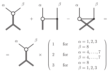
Figure 1: Graphical computation of the Wess–Zumino current quantity $N(\tau)$

For the minimal SU(3)_f extended Skyrme model polar components of the “killing” vectors $\xi_{i}^{\alpha}\,,\,\eta_{i}^{\alpha}$, and ${\bf{\cal U}}_{\alpha}^{\beta}$ are computed and presented in tabular forms, 1–3.

Table 1: “Killing” vectors ${\xi}_{i}^{j}$ and ${\eta}_{i}^{j}$ in polar coordinates

$i$	$r$	$\theta$	$\phi$
$\xi^{1}_{i}$	$2\,F^{\prime}\,\sin{\theta}\,\cos{\phi}$	$\sin 2F\,\cos{\theta}\,\cos{\phi}+$	$-\sin 2F\,\sin{\theta}\,\sin{\phi}+$
		$2\sin^{2}F\,\sin{\phi}$	$\sin^{2}F\,\sin 2{\theta}\,\cos{\phi}$
$\xi^{2}_{i}$	$2F^{\prime}\,\sin{\theta}\,\sin{\phi}$	$\sin^{2}F\,\cos{\theta}\,\sin{\phi}-$	$\sin 2F\,\sin{\theta}\,\cos{\phi}+$
		$2\sin^{2}F\,\cos{\phi}$	$\sin^{2}F\,\sin 2{\theta}\,\sin{\phi}$
$\xi^{3}_{i}$	$2\,F^{\prime}\,\cos{\theta}$	$-\sin 2F\,\sin{\theta}$	$-2\sin^{2}F\,\sin^{2}{\theta}$
$\eta^{1}_{i}$	$2\,F^{\prime}\,\sin{\theta}\,\cos{\phi}$	$\sin 2F\,\cos{\theta}\,\cos{\phi}-$	$-\sin 2F\,\sin{\theta}\,\sin{\phi}-$
		$2\sin^{2}F\,\sin{\phi}$	$\sin^{2}F\,\sin 2{\theta}\,\cos{\phi}$
$\eta^{2}_{i}$	$2F^{\prime}\,\sin{\theta}\,\sin{\phi}$	$\sin^{2}F\,\cos{\theta}\,\sin{\phi}+$	$\sin 2F\,\sin{\theta}\,\cos{\phi}-$
		$2\sin^{2}F\,\cos{\phi}$	$\sin^{2}F\,\sin 2{\theta}\,\sin{\phi}$
$\eta^{3}_{i}$	$2\,F^{\prime}\,\cos{\theta}$	$-\sin 2F\,\sin{\theta}$	$2\sin^{2}F\,\sin^{2}{\theta}$

${\xi}_{i}^{A}=-i{\rm Tr}((\partial_{i}{\cal U}){\cal U}^{\dagger}\lambda^{A})\>;\>{\eta}_{i}^{A}=-i{\rm Tr}({\cal U}^{\dagger}(\partial_{i}{\cal U})\lambda^{A})\>;$

$A=1,2,3,8\>;\>{\xi}_{i}^{8}={\eta}_{i}^{8}=0$

Table 2: “Killing” vectors ${\cal U}_{\alpha}^{\beta}=\frac{1}{2}\rm Tr(\lambda_{\alpha}{\cal U}^{\dagger}\lambda^{\beta}{\cal U})$ in polar coordinates

$\beta$	$1$	$2$	$3$
${\cal U}_{1}^{\beta}$	$\cos^{2}F-\sin^{2}F\cos^{2}{\theta}+$	$\sin 2F\cos{\theta}+$	$-\sin 2F\,\sin{\theta}\,\sin{\phi}+$
	$\sin^{2}F\,\sin^{2}{\theta}\,\cos 2{\phi}$	$\sin^{2}F\,\sin^{2}{\theta}\,\sin 2{\phi}$	$2\sin^{2}F\,\sin 2{\theta}\,\cos{\phi}$
${\cal U}_{2}^{\beta}$	$-\sin 2F\,\cos{\theta}+$	$\cos^{2}F-\sin^{2}F\cos^{2}{\theta}-$	$\sin 2F\,\sin{\theta}\,\cos{\phi}+$
	$\sin^{2}F\,\sin^{2}{\theta}\,\sin 2{\phi}$	$-\sin^{2}F\,\sin^{2}{\theta}\,\cos 2{\phi}-$	$\sin^{2}F\,\sin 2{\theta}\,\sin{\phi}$
${\cal U}_{3}^{\beta}$	$\sin 2F\,\sin{\theta}\,\sin{\phi}+$	$-\sin 2F\,\sin{\theta}\,\cos{\phi}+$	$1-2\sin^{2}F\,\sin^{2}{\theta}$
	$\sin^{2}F\,\sin 2{\theta}\,\cos{\phi}$	$\sin^{2}F\,\sin 2{\theta}\,\sin{\phi}$

Other components are:   ${\cal U}_{\alpha}^{\beta}=0\;\rm for\;\alpha=1,2,3\;;\;\beta=4,5,6,7,8$

Table 3: “Killing” vectors ${\cal U}_{\alpha}^{\beta}=\frac{1}{2}\rm Tr(\lambda_{\alpha}{\cal U}^{\dagger}\lambda^{\beta}{\cal U})$ in polar coordinates

$\beta$	$4$	$5$	$6$	$7$
${\cal U}_{4}^{\beta}$	$\cos F$	$\sin F\cos{\theta}$	$\sin F\sin{\theta}\sin{\phi}$	$\sin F\,\sin{\theta}\,\cos{\phi}$
${\cal U}_{5}^{\beta}$	$-\sin F\,\cos{\theta}$	$\cos F$	$-\sin F\,\sin{\theta}\,\cos{\phi}$	$\sin F\sin{\theta}\sin{\phi}$
${\cal U}_{6}^{\beta}$	$-\sin F\sin{\theta}\sin{\phi}$	$\sin F\,\sin{\theta}\,\cos{\phi}$	$\cos F$	$-\sin F\cos{\theta}$
${\cal U}_{7}^{\beta}$	$-\sin F\sin{\theta}\cos{\phi}$	$-\sin F\,\sin{\theta}\,\sin{\phi}$	$\sin F\cos{\theta}$	$\cos{\theta}$

Other components are: ${\cal U}_{\alpha}^{\beta}=0\;\rm for\;\alpha=4,5,6,7,8\;;\;\beta=1,2,3\;\&\;{\cal U}_{8}^{8}=1$

II.3 Arctan ansatz as the ${\rm SU(3)_{f}}$ profile function F(r) and dynamics of the SU(3)_f symmetry breaking

For the SU(3)_f extension (9) of the Skyrme Lagrangian (1), we use a new set of parameters ${\hat{x}},{\beta}^{\prime},{\delta}^{\prime}$ introduced in Ref. wei . The symmetry breaker ${\hat{x}}$ was constructed systematically from the QCD mass term. The $\delta^{\prime}$ term is required to split pseudoscalar meson masses, while the $\beta^{\prime}$ term is required to split pseudoscalar decay constants wei :

$$\beta^{\prime}=\frac{f^{2}_{K}-f^{2}_{\pi}}{4(1-{\hat{x}})},\;\;\delta^{\prime}=\frac{m^{2}_{\pi}f^{2}_{\pi}}{4}=\frac{m^{2}_{K}f^{2}_{K}}{2(1+{\hat{x}})},\;\;{\hat{x}}=\frac{2m^{2}_{K}f^{2}_{K}}{m^{2}_{\pi}f^{2}_{\pi}}-1.$$ (24)

Considering the above symmetry breaking parameters we are introducing three different dynamical assumptions, based on the SB (11), producing three fits which are going to be used further on in our numerical analysis:

$$({\rm i}) \;\hskip 0.56905ptm_{\pi}=m_{K}=0,\;\,f_{\pi}=f_{K}=93\;\,{\rm MeV}\;\Longrightarrow\;\,{\hat{x}}=1,\;\,\beta^{\prime}=\delta^{\prime}=0;$$

$$({\rm ii}) \;\hskip 0.28453ptm_{\pi}=138,\;\,m_{K}=495,\;\,f_{\pi}=f_{K}=93,\,\;{\rm MeV}\;\Longrightarrow\,\hskip 14.22636pt{\hat{x}}=24.73,\,\;\beta^{\prime}=0,\,\;\delta^{\prime}=4.12\,\times 10^{7},\,{\rm MeV}^{4};$$

$$({\rm iii}) \,m_{\pi}=138,\,\;m_{K}=495,\,\;f_{\pi}=93,\,\;f_{K}=113\,{\rm MeV}\Longrightarrow{\hat{x}}=36.97,\;\,\beta^{\prime}=-28.6\;\,{\rm MeV}^{2},\,\;\delta^{\prime}=4.12\,\times 10^{7},\,{\rm MeV}^{4}.$$

Fit (i) corresponds to the SU(3)_f chiral limit. For the numerical results, which are going to be presented in Tables 4-9, we choose typical range of the Skyrme charge values $3.0\;\leq\;e\;\leq\;5.0$. The reason for this lies in the fact that in the most realistic case (iii), $e=3.4,\;4.2,\;4.4,\;4.7$, gives the best fit for axial-vector coupling $g_{A}$, the octet-decuplet mass splitting $\Delta_{1}$, and for the penta-quark masses $M_{\Theta^{+}}$ and $M_{\Xi^{--}_{3/2}}$, respectively.

Substituting (12) into (9) we obtain classical soliton mass ${\cal M}_{\rm csol}$ containing the symmetry breakers $\hat{x}$, $\beta^{\prime}$ and $\delta^{\prime}$. Owing to their presence in ${\cal M}_{\rm csol}$ the dimensionless size of skyrmion $x_{0}$ is affected, i.e. instead of being a constant it becomes a complicated function of $e$, $m_{\pi}$, $f_{\pi}$, $m_{K}$, $f_{K}$, or via Eqs. (24) a function of $e$, $f_{\pi}$, $\beta^{\prime}$, and $\delta^{\prime}$: $x_{0}\longrightarrow x_{0}^{SB}=x_{0}^{SB}(e,f_{\pi},\beta^{\prime},\delta^{\prime})\equiv x^{\prime}_{0}$. The analytical expression for the SU(3)_f extended classical soliton mass:

$${\cal M}_{\rm csol}[F] = 2\pi\frac{f_{\pi}}{e}\int_{0}^{\infty}dx\left\{\left(x^{2}{F^{\prime}}^{2}+2\sin^{2}F\right)+\sin^{2}F\left(2{F^{\prime}}^{2}+\frac{\sin^{2}F}{x^{2}}\right)\right.$$ (26)

$$\left.+\frac{8}{f^{2}_{\pi}}(1-\cos F)\left[{\beta}^{\prime}\left(x^{2}{F^{\prime}}^{2}+2\sin^{2}F\right)+\frac{{\delta}^{\prime}}{e^{2}f^{2}_{\pi}}x^{2}\right]\right\}$$

$$= 3{\sqrt{2}}{\pi}^{2}\left[x^{\prime}_{0}+\frac{15}{16x^{\prime}_{0}}+\frac{2}{f^{2}_{\pi}}\left(3{\beta}^{\prime}x^{\prime}_{0}+\frac{4}{3}\frac{\delta^{\prime}}{e^{2}f^{2}_{\pi}}x^{\prime 3}_{0}\right)\right]\frac{f_{\pi}}{e},$$

we are using next to obtain dimensionless size of skyrmion $x^{\prime}_{0}$. Minimizing ${\cal M}_{\rm csol}$ with respect to $x^{\prime}_{0}$, we have found :

$${x^{\prime}_{0}}^{2}=\frac{15}{8}\left[1+\frac{6\beta^{\prime}}{f^{2}_{\pi}}+\sqrt{\left(1+\frac{6\beta^{\prime}}{f^{2}_{\pi}}\right)^{2}+\frac{30\delta^{\prime}}{e^{2}f^{4}_{\pi}}}\;\right]^{-1},$$ (27)

which analytically describes the dynamics of skyrmion internal SU(3)_f symmetry breaking effects. This is our main result and it is clear from the above equation that a skyrmion effectively shrinks when the Skyrme charge $e$ receives smaller values and it shrinks more when one “switches on” symmetry breaking effects. The influence of the internal skyrmion dynamics, due to the symmetry breaking effects, on the nucleon axial-vector current, the mass spectrum and the mass differences are going to be presented in tabular form.

II.4 Nucleon axial-vector coupling, moments of inertia, the 8, 10, $\overline{\bf 10}$, ${\bf 27}_{3/2}$ mass spectrums and
the higher SU(3)_f representation mass splittings

Including the previously introduced arctan ansatz for the profile function $F(r)$, in the minimal SU(3)_f extended Skyrme model currents (17), we first compute the analytical expressions for the nucleon axial-vector coupling constant $g_{A}(x^{\prime}_{0})$, the moment of inertia for rotation in coordinate space $\lambda_{c}(x^{\prime}_{0})$, the moment of inertia for flavor rotations in the direction of the strange degrees of freedom, except for the eight directions $\lambda_{s}(x^{\prime}_{0})$ and the SU(3)_f symmetry breaking quantity $\gamma(x^{\prime}_{0})$ relevant to evaluate the higher SU(3)_f representation mass splittings as well as the 8, 10, $\overline{\bf 10}$ and ${\bf 27}_{3/2}$ absolute mass spectrum wei ; prat2 , respectively.

$$g_{A}[F] = \frac{\pi}{e^{2}}\int_{0}^{\infty}dx\left\{\left[F^{\prime}\left(x^{2}+2\sin^{2}F\right)+x\sin 2F\left(1+{F^{\prime}}^{2}\right)+\frac{\sin^{2}F}{x}\sin 2F\right]\frac{-7}{30}\right.$$ (28)

$$\left.+\frac{4{\beta}^{\prime}}{3f^{2}_{\pi}}\left(1-\hat{x}\right)(1-\cos F)\left[\left(\frac{2\sin F}{x}(1+2\cos F)+F^{\prime}\right)\frac{-49}{300}+\left(\frac{2\sin F}{x}-F^{\prime}\right)\frac{-1}{75}\right]\right.$$

$$\left.+\frac{eN_{c}}{12{\pi}^{2}f_{\pi}\lambda_{s}[F]}(1-\cos F)\frac{\sin F}{x}\left(\frac{\sin F}{x}-2F^{\prime}\right)\frac{14}{30}\right\}$$

$$= \frac{14\pi}{15e^{2}}\left(2x^{\prime 2}_{0}+\pi\right)+(1-{\hat{x}})\frac{16\pi\beta^{\prime}}{225e^{2}f^{2}_{\pi}}{x^{\prime}}_{0}^{2}+\frac{7\sqrt{2}N_{c}}{192ef_{\pi}}\frac{x_{0}^{\prime}}{\lambda_{s}(x_{0}^{\prime})},$$

$$\lambda_{c}[F] = \frac{8\pi}{3e^{3}f_{\pi}}\int_{0}^{\infty}dx\sin^{2}F\left\{x^{2}\left(1+{F^{\prime}}^{2}+\frac{8{\beta}^{\prime}}{f^{2}_{\pi}}(1-\cos F)\right)+\sin^{2}F\right\}$$ (29)

$$= \frac{\sqrt{2}\pi^{2}}{3e^{3}f_{\pi}}\left[6\left(1+2\frac{\beta^{\prime}}{f^{2}_{\pi}}\right)x^{\prime 3}_{0}+\frac{25}{4}x^{\prime}_{0}\right],$$

$$\lambda_{s}[F] = \frac{\pi}{2e^{3}f_{\pi}}\int_{0}^{\infty}dx(1-\cos F)\left\{x^{2}\left[4+{F^{\prime}}^{2}-\frac{16{\beta}^{\prime}}{f^{2}_{\pi}}\left({\hat{x}}+\cos F\right)\right]+2\sin^{2}F\right\}$$ (30)

$$= \frac{\sqrt{2}\pi^{2}}{4e^{3}f_{\pi}}\left[4\left(1-2\left(1+2{\hat{x}}\right)\frac{\beta^{\prime}}{f^{2}_{\pi}}\right){x^{\prime}}^{3}_{0}+\frac{9}{4}x^{\prime}_{0}\right],$$

$$\gamma[F] = \frac{32\pi}{3}\frac{{\hat{x}}-1}{e^{3}f^{3}_{\pi}}\int_{0}^{\infty}dx\left\{{\delta}^{\prime}x^{2}(1-\cos F)-e^{2}f^{2}_{\pi}{\beta}^{\prime}\cos F\left(x^{2}{F^{\prime}}^{2}+2\sin^{2}F\right)\right\}$$ (31)

$$= 4\sqrt{2}{\pi}^{2}\frac{1-{\hat{x}}}{ef_{\pi}}\left[{\beta}^{\prime}x^{\prime}_{0}-\frac{4}{3}\frac{\delta^{\prime}}{e^{2}f^{2}_{\pi}}x^{\prime 3}_{0}\right].$$

Table 4: The SU(3)_f Skyrme model dimensionless size of skyrmion $x^{\prime}_{0}$, axial-vector coupling constant $g_{A}$, the rotational moments of inertia $\lambda_{c(s)}$ (GeV^-1) and the SB quantity $\gamma$ (GeV), for fits (i), (ii) and (iii). For fit (i) $x^{\prime}_{0}\equiv x_{0}=\frac{\sqrt{15}}{4}$ and $\gamma=0$.

${\rm Fits}$		$({\rm i})$				$({\rm ii})$					$({\rm iii})$
$e$	$g_{A}$	$\lambda_{c}$	$\lambda_{s}$	$x_{0}^{\prime}$	$g_{A}$	$\lambda_{c}$	$\lambda_{s}$	$\gamma$	$x_{0}^{\prime}$	$g_{A}$	$\lambda_{c}$	$\lambda_{s}$	$\gamma$
$3.0$	$1.701$	$21.304$	$8.073$	$0.8359$	$1.558$	$16.172$	$5.860$	$1.956$	$0.8408$	$1.548$	$16.300$	$7.572$	$3.192$
$3.2$	$1.512$	$17.554$	$6.652$	$0.8465$	$1.399$	$13.635$	$4.960$	$1.674$	$0.8517$	$1.386$	$13.750$	$6.429$	$2.751$
$3.4$	$1.358$	$14.635$	$5.546$	$0.8561$	$1.268$	$11.602$	$4.235$	$1.444$	$0.8615$	$1.251$	$11.705$	$5.504$	$2.388$
$3.6$	$1.231$	$12.329$	$4.672$	$0.8646$	$1.159$	$9.953$	$3.644$	$1.253$	$0.8703$	$1.140$	$10.046$	$4.748$	$2.088$
$3.8$	$1.125$	$10.483$	$3.972$	$0.8723$	$1.068$	$8.602$	$3.158$	$1.094$	$0.8782$	$1.046$	$8.685$	$4.123$	$1.836$
$4.0$	$1.038$	$8.988$	$3.406$	$0.8792$	$0.992$	$7.483$	$2.754$	$0.960$	$0.8854$	$0.967$	$7.559$	$3.603$	$1.624$
$4.1$	$0.999$	$8.346$	$3.163$	$0.8824$	$0.959$	$6.996$	$2.577$	$0.902$	$0.8887$	$0.932$	$7.068$	$3.375$	$1.531$
$4.2$	$0.964$	$7.764$	$2.942$	$0.8855$	$0.928$	$6.550$	$2.415$	$0.847$	$0.8918$	$0.899$	$6.618$	$3.166$	$1.444$
$4.4$	$0.903$	$6.753$	$2.559$	$0.8911$	$0.874$	$5.764$	$2.130$	$0.751$	$0.8976$	$0.842$	$5.827$	$2.796$	$1.291$
$4.6$	$0.851$	$5.910$	$2.239$	$0.8962$	$0.830$	$5.099$	$1.887$	$0.669$	$0.9029$	$0.794$	$5.156$	$2.481$	$1.159$
$4.8$	$0.809$	$5.201$	$1.971$	$0.9009$	$0.792$	$4.532$	$1.680$	$0.598$	$0.9076$	$0.753$	$4.583$	$2.212$	$1.045$
$5.0$	$0.773$	$4.602$	$1.744$	$0.9051$	$0.761$	$4.045$	$1.502$	$0.537$	$0.9122$	$0.718$	$4.092$	$1.979$	$0.946$
$\rm Exp.$	$1.26$	$-$	$-$	$-$	$1.26$	$-$	$-$	$-$	$-$	$1.26$	$-$	$-$	$-$

The last remaining quantity, $\gamma$, is an important coefficient in the symmetry breaking piece ${\cal L}_{\rm SB}=-\frac{1}{2}\gamma(1-D_{88})$ of a total collective Hamiltonian (16) and is linear in the symmetry breaking parameter $(1-{\hat{x}})$. Switching off SU(3)_f symmetry breaking and in the chiral limit $\beta^{\prime}=\delta^{\prime}=0$, $x_{0}^{\prime}\longrightarrow x_{0}=\sqrt{15}/4$, the $\lambda_{c}/\lambda_{s}$ becomes 95/36 and $\gamma=0$. For $e=4$, all above expressions are in very good agreement with the values (2.48) from Ref. wei where fine tuning effects, like vector-meson contributions, the so-called static fluctuation, vibrations of Kaons, etc., wei are taken into account. For example, $\beta^{2}\equiv\lambda_{s}(x_{0}^{\prime})=3.62$ GeV^-1 is very close to the value of $3.52$ GeV^-1 mentioned in the discussion below Eq. (2.48) on p. 2440 of Ref. wei . This represents an implicit proof that the inclusion of the fine tuning effects does not change our results dramatically and is one of our main reasons to concentrate on the axial-vector coupling and moments of inertia only. Their numerical values as a functions of $e$ are given in Table 4, while graphical displays are given for cases (i), (ii) and (iii) in Figures 2, 3 and 4, respectively.

Moments of inertia we need to predict the 8, 10, $\overline{\bf 10}$ and 27 mass spectrums and the higher SU(3)_f representation mass splittings, while the evaluation of nucleon axial-vector coupling $g_{A}$ in this paper serves only as a consistency check of the approach as a whole. Inspection of our Table 4 case (iii), shows that $g_{A}=0.97$ for $e=4$, agrees within 1% with value $g_{A}=0.98$ from page 2449 in Ref. wei . Other quantities, like magnetic moments and charge radii, for the minimal SU(3)_f extended Skyrme model, behave in the same way and it is not necessary to present them here. For them we simply refer to the complete calculation presented in Table 2.2 of Ref. wei . However, for the sake of comparison with the SU(2)_f results (6-8), and because we are also interested in the influence of the SB dynamics (27) on the leading SU(2)_f terms of charge radii and magnetic moments of nucleons, we next estimate the isoscalar and the isovector components of magnetic moments of proton and neutron, nucleon isoscalar mean radius $R_{I}$, and isoscalar magnetic mean radius $R_{M}$, and present them as functions of $e$ and for fits (II.3), in Table 5.

$${\mu}_{p\choose n}[F] = \frac{m_{p\choose n}}{3}\left[\frac{2{x^{\prime}}_{0}^{2}}{\pi e^{2}f^{2}_{\pi}\lambda_{c}(x_{0}^{\prime})}\pm\lambda_{c}(x_{0}^{\prime})\right],$$ (32)

$$R^{2}_{I}[F] = \frac{-2}{\pi e^{2}f_{\pi}^{2}}\int dx\,x^{2}F^{\prime}\sin^{2}F=\frac{4}{\pi}\frac{x^{\prime 2}_{0}}{e^{2}f_{\pi}^{2}},\;\;R^{2}_{M}[F]=\frac{-1}{2x^{\prime 2}_{0}e^{2}f_{\pi}^{2}}\int dx\,x^{4}F^{\prime}\sin^{2}F=\frac{3\pi}{4}\frac{x^{\prime 2}_{0}}{e^{2}f_{\pi}^{2}}.$$ (33)

Table 5: The SU(2)_f Skyrme model isoscalar mean radii $R_{I(M)}$(fm) and the magnetic moments of the proton and the neutron, in terms of the nucleon Bohr magneton $[\mu_{B}]$, as functions of charge $e$ and for fits (i), (ii) and (iii).

${\rm Fits}$		$({\rm i})$					$({\rm ii})$					$({\rm iii})$
$e$	$R_{I}$	$R_{M}$	$\mu_{p}$	$\mu_{n}$	$x^{\prime}_{0}$	$R_{I}$	$R_{M}$	$\mu_{p}$	$\mu_{n}$	$x^{\prime}_{0}$	$R_{I}$	$R_{M}$	$\mu_{p}$	$\mu_{n}$
$3.0$	$0.773$	$1.051$	$6.774$	$-6.563$	$0.8359$	$0.667$	$0.907$	$5.167$	$-4.956$	$0.8408$	$0.671$	$0.913$	$5.207$	$-4.996$
$3.2$	$0.724$	$0.985$	$5.609$	$-5.380$	$0.8465$	$0.633$	$0.862$	$4.381$	$-4.154$	$0.8517$	$0.637$	$0.867$	$4.418$	$-4.189$
$3.4$	$0.682$	$0.928$	$4.703$	$-4.459$	$0.8561$	$0.603$	$0.820$	$3.753$	$-3.509$	$0.8615$	$0.607$	$0.825$	$3.786$	$-3.541$
$3.6$	$0.644$	$0.876$	$3.990$	$-3.728$	$0.8646$	$0.575$	$0.782$	$3.245$	$-2.985$	$0.8703$	$0.579$	$0.787$	$3.275$	$-3.014$
$3.8$	$0.610$	$0.830$	$3.420$	$-3.142$	$0.8723$	$0.550$	$0.748$	$2.830$	$-2.554$	$0.8782$	$0.553$	$0.753$	$2.857$	$-2.580$
$4.0$	$0.580$	$0.788$	$2.960$	$-2.666$	$0.8792$	$0.527$	$0.716$	$2.488$	$-2.196$	$0.8854$	$0.530$	$0.721$	$2.513$	$-2.219$
$4.1$	$0.565$	$0.769$	$2.763$	$-2.461$	$0.8824$	$0.515$	$0.701$	$2.340$	$-2.039$	$0.8887$	$0.519$	$0.706$	$2.363$	$-2.061$
$4.2$	$0.552$	$0.751$	$2.585$	$-2.275$	$0.8855$	$0.505$	$0.687$	$2.204$	$-1.896$	$0.8918$	$0.508$	$0.692$	$2.226$	$-1.917$
$4.4$	$0.527$	$0.717$	$2.276$	$-1.950$	$0.8911$	$0.485$	$0.660$	$1.966$	$-1.642$	$0.8976$	$0.488$	$0.664$	$1.986$	$-1.661$
$4.6$	$0.504$	$0.686$	$2.020$	$-1.679$	$0.8962$	$0.466$	$0.635$	$1.766$	$-1.426$	$0.9020$	$0.470$	$0.639$	$1.784$	$-1.443$
$4.8$	$0.483$	$0.657$	$1.806$	$-1.449$	$0.9009$	$0.449$	$0.611$	$1.596$	$-1.241$	$0.9076$	$0.453$	$0.616$	$1.613$	$-1.256$
$5.0$	$0.464$	$0.631$	$1.626$	$-1.254$	$0.9051$	$0.433$	$0.590$	$1.451$	$-1.081$	$0.9122$	$0.437$	$0.594$	$1.467$	$-1.095$
$\rm Exp.$	$0.72$	$0.81$	2.79	$-1.91$	$-$	$0.72$	$0.81$	2.79	$-1.91$	$-$	$0.72$	$0.81$	2.79	$-1.91$

To obtain the 8, 10, $\overline{\bf 10}$ and ${\bf 27}_{3/2}$ mass spectrums we use the mass formula (16) and find

$$M^{\bf 8}_{B}[F] = {\cal M}_{\bf 8}-\frac{1}{2}\gamma(x^{\prime}_{0})\;\delta^{\bf 8}_{B},\;\;M^{\bf 10}_{B}[F]={\cal M}_{\bf 8}+\frac{3}{2\lambda_{c}(x_{0}^{\prime})}-\frac{1}{2}\gamma(x^{\prime}_{0})\;\delta^{\bf 10}_{B},$$ (34)

$$M^{\overline{\bf 10}}_{B}[F] = {\cal M}_{\bf 8}+\frac{3}{2\lambda_{s}(x_{0}^{\prime})}-\frac{1}{2}\gamma(x^{\prime}_{0})\;\delta^{\overline{\bf 10}}_{B},\;\;{\rm M}^{\bf 27}_{B}[F]={\cal M}^{\bf 8}+\frac{3}{2\lambda_{c}(x_{0}^{\prime})}+\frac{1}{\lambda_{s}(x_{0}^{\prime})}-\frac{1}{2}\gamma(x_{0}^{\prime})\;\delta^{\bf 27}_{B},$$ (35)

where the experimental octet mean mass ${\cal M}^{\bf 8}=\frac{1}{8}\sum_{B=1}^{\bf 8}M^{\bf 8}_{B}=1151$ MeV was used instead of

$${\cal M}^{\bf 8}={\cal M}_{\rm csol}(x_{0}^{\prime})+\frac{3}{2\lambda_{c}(x_{0}^{\prime})}.$$ (36)

The reason is simply because nowadays everybody agrees that the SU(3)_f extended Skyrme model classical soliton mass ${\cal M}_{\rm csol}$ receives to large value producing unrealistic baryonic mass spectrum. From measurements we also know ${\cal M}^{\bf 10}=\frac{1}{10}\sum^{10}_{B=1}M^{\bf 10}_{B}=1382$ MeV rpp . The splitting constants $\delta^{\bf 8}_{B}$, $\delta^{\bf 10}_{B}$ and $\delta^{\overline{\bf 10}}_{B}$ are given in Eqs. (5) to (18) of Ref. Ell , while $\delta^{\bf 27}_{B}$ could be found in Table 1. of Ref. WM .

Equations (34,35) assume equal spacing between multiplets. From the existing experiments penta1 –penta6 ($M_{\Theta^{+}}=1540$ MeV and $M_{\Xi^{--}_{3/2}}=1861$ MeV) we estimate that spacing to be $\overline{\delta}=(1861-1540)/3=107$ MeV. Next we estimate masses of antidecuplets $M_{N^{*}}=1647$ MeV, $M_{\Sigma_{\overline{10}}}=1754$ MeV and the ${\overline{\bf 10}}$ mean mass ${\cal M}_{\overline{\bf 10}}=\frac{1}{10}\sum^{10}_{B=1}M^{\overline{\bf 10}}_{B}=1754$ MeV, and using them bonafide as an “experimental” values further on. From the expressions (34,35) it is clear that in the SU(3)_f symmetric case and in the chiral limit the 8, 10, $\overline{\bf 10}$ and ${\bf 27}_{3/2}$, absolute masses of each member of the multiplet become equal for each fixed $e$: $\rm N=\Lambda=\Sigma=\Xi\equiv M^{\bf 8}_{B}$, $\Delta=\Sigma^{*}=\Xi^{*}=\Omega\equiv M^{\bf 10}_{B}$, $\Theta^{+}=\rm N^{*}=\Sigma_{\overline{10}}=\Xi^{--}_{3/2}\equiv M^{\overline{\bf 10}}_{B}$ and $\Theta_{1}={\rm N}^{*}_{\frac{3}{2}}=\Sigma_{2}={\rm N}^{*}_{\frac{1}{2}}=\Sigma_{1}=\Lambda^{*}=\Xi^{*}_{\frac{3}{2}}=\Xi^{*}_{\frac{1}{2}}=\Omega_{1}\equiv M^{\bf 27}_{B}$. For example, with ${\cal M}_{\bf 8}=1151$ MeV as an input and for $e=4.7$ we would have $\left[M^{\bf 8}_{B},M^{\bf 10}_{B},M^{\overline{\bf 10}}_{B},M^{\bf 27}_{B}\right]=[1151,1422,1865,1898]$ MeV. Numerics for the 8, 10, $\overline{\bf 10}$ and ${\bf 27}_{3/2}$ mass spectrums in the SU(3)_f Skyrme model as functions of charge $4\leq e\leq 5$ and for fits (ii) and (iii) are given in Tables 6 and 7, respectively. The Skyrme charge $e$ and the SB effects dependences of the mass spectrums are very transparently presented in Figures 5, 6 and 7, respectively. Note that in the computations of the mean masses ${\cal M}^{\bf 8}$,…, the sum of $D_{88}$ diagonal elements over all components of irreducible representations cancels out because of the properties of the SU(3) Clebsch-Gordan coefficients desw ; fin . In the above notation we are following Fig. 4 from Ref.Ell as close as possible. However, the $\overline{\bf 10}$-plet members $\Theta$, $\Sigma$ and $\Xi_{3/2}$ we mark as $\Theta^{+}$, $\Sigma_{\overline{\bf 10}}$ and $\Xi^{--}_{3/2}$, respectively. The $\Xi$ isoquartet and isodoublet from the ${\bf 27}_{3/2}$ we mark as $\Xi^{*}_{\frac{3}{2}}$ and $\Xi^{*}_{\frac{1}{2}}$, to distinguish them from the $\Xi$ isoquartet and isodoublet from the $\overline{\bf 10}$. We also mark the ${\bf 27}_{3/2}$-plet isosinglet as $\Lambda^{*}$.

Table 6: The 8 and 10 mass spectrums (MeV) as functions of charge $e$ and for fits (ii)and (iii). The experimental numbers for 8 and 10 masses were used from rpp

.

${\rm Fits}$				$({\rm ii})$								$({\rm iii})$
$e$	$\rm N$	$\Lambda$	$\Sigma$	$\Xi$	$\Delta$	$\Sigma^{*}$	$\Xi^{*}$	$\Omega$	$\rm N$	$\Lambda$	$\Sigma$	$\Xi$	$\Delta$	$\Sigma^{*}$	$\Xi^{*}$	$\Omega$
$4.0$	$1007$	$1103$	$1199$	$1247$	$1291$	$1351$	$1411$	$1472$	$907$	$1070$	$1232$	$1313$	$1248$	$1350$	$1451$	$1552$
$4.1$	$1016$	$1106$	$1196$	$1241$	$1309$	$1365$	$1422$	$1478$	$921$	$1074$	$1228$	$1304$	$1268$	$1363$	$1459$	$1555$
$4.2$	$1024$	$1109$	$1193$	$1236$	$1327$	$1380$	$1433$	$1486$	$934$	$1079$	$1223$	$1295$	$1287$	$1378$	$1468$	$1558$
$4.4$	$1038$	$1113$	$1189$	$1226$	$1364$	$1411$	$1458$	$1505$	$957$	$1086$	$1216$	$1280$	$1328$	$1408$	$1489$	$1570$
$4.6$	$1051$	$1118$	$1184$	$1218$	$1403$	$1445$	$1487$	$1529$	$977$	$1093$	$1209$	$1267$	$1370$	$1442$	$1514$	$1587$
$4.8$	$1061$	$1121$	$1181$	$1211$	$1445$	$1482$	$1519$	$1557$	$994$	$1099$	$1203$	$1255$	$1413$	$1478$	$1544$	$1609$
$5.0$	$1071$	$1124$	$1178$	$1205$	$1488$	$1522$	$1555$	$1589$	$1009$	$1104$	$1198$	$1246$	$1458$	$1518$	$1577$	$1636$
$\rm Exp.$	$939$	$1116$	$1193$	$1318$	$1232$	$1385$	$1530$	$1672$	$939$	$1116$	$1193$	$1318$	$1232$	$1385$	$1530$	$1672$

Table 7: The $\overline{\bf 10}$ and 27_3/2 mass spectrums (MeV) as functions of Skyrme charge $e$ and fits (ii), (iii). The $\Theta^{+}$ and $\Xi^{--}_{3/2}$ experimental masses can be find in penta1 –penta6 .

${\rm Fits}$	$e$	$\Theta^{+}$	$\rm N^{*}$	$\Sigma_{\overline{10}}$	$\Xi^{--}_{3/2}$	$\Theta_{1}$	$\rm N^{*}_{\frac{3}{2}}$	$\Sigma_{2}$	$\rm N^{*}_{\frac{1}{2}}$	$\Sigma_{1}$	$\Lambda^{*}$	$\Xi^{*}_{\frac{3}{2}}$	$\Xi^{*}_{\frac{1}{2}}$	$\Omega_{1}$
	$4.0$	$1576$	$1636$	$1696$	$1756$	$1646$	$1659$	$1671$	$1697$	$1723$	$1749$	$1749$	$1788$	$1826$
	$4.1$	$1620$	$1677$	$1733$	$1789$	$1689$	$1701$	$1713$	$1737$	$1761$	$1786$	$1786$	$1822$	$1858$
$(\rm{ii})$	$4.2$	$1666$	$1719$	$1772$	$1825$	$1734$	$1745$	$1756$	$1779$	$1802$	$1824$	$1824$	$1858$	$1892$
	$4.4$	$1761$	$1808$	$1855$	$1902$	$1827$	$1837$	$1847$	$1867$	$1887$	$1908$	$1908$	$1938$	$1968$
	$4.6$	$1862$	$1904$	$1946$	$1988$	$1927$	$1936$	$1945$	$1963$	$1981$	$1999$	$1999$	$2026$	$2053$
	$4.8$	$1969$	$2007$	$2044$	$2082$	$2035$	$2043$	$2051$	$2067$	$2083$	$2099$	$2099$	$2123$	$2147$
	$5.0$	$2083$	$2116$	$2150$	$2183$	$2149$	$2157$	$2164$	$2178$	$2193$	$2207$	$2207$	$2229$	$2250$
	$4.0$	$1364$	$1466$	$1567$	$1668$	$1511$	$1533$	$1554$	$1598$	$1642$	$1685$	$1685$	$1750$	$1816$
	$4.1$	$1404$	$1500$	$1595$	$1691$	$1550$	$1571$	$1591$	$1532$	$1673$	$1714$	$1714$	$1776$	$1837$
$(\rm{iii})$	$4.2$	$1444$	$1535$	$1625$	$1715$	$1590$	$1610$	$1629$	$1668$	$1706$	$1745$	$1745$	$1803$	$1861$
	$4.4$	$1526$	$1607$	$1687$	$1768$	$1674$	$1691$	$1708$	$1743$	$1778$	$1812$	$1812$	$1864$	$1916$
	$4.6$	$1611$	$1683$	$1755$	$1828$	$1762$	$1778$	$1793$	$1824$	$1855$	$1886$	$1886$	$1933$	$1979$
	$4.8$	$1699$	$1764$	$1829$	$1894$	$1856$	$1870$	$1884$	$1912$	$1940$	$1968$	$1968$	$2010$	$2052$
	$5.0$	$1791$	$1850$	$1909$	$1968$	$1955$	$1969$	$1981$	$2006$	$2031$	$2057$	$2057$	$2094$	$2133$
$\rm Exp.$		$1540$	$-$	$-$	$1861$	$-$	$-$	$-$	$-$	$-$	$-$	$-$	$-$	$-$

The predictions for higher SU(3)_f representations mass splittings are in order. The mass splittings $\Delta_{i}[F],\,i=1,...,4$, for the multiplets ${\bf 8}_{J=1/2}$, ${\bf 10}_{J=3/2}$, $\overline{\bf 10}_{J=1/2}$, ${\bf 27}_{J=3/2}$ and ${\bf 35}_{J=5/2}$ expressed by the following simple relations:

$${\Delta}_{1}[F] = {\cal M}^{\bf 10}-{\cal M}^{\bf 8}=\frac{3}{2\lambda_{c}(x_{0}^{\prime})}\equiv{\Delta}_{1},\;\;\;\,\hskip 5.69054pt{\Delta}_{2}[F]={\cal M}^{\overline{\bf 10}}-{\cal M}^{\bf 8}=\frac{3}{2\lambda_{s}(x_{0}^{\prime})}\equiv{\Delta}_{2},$$

$${\Delta}_{3}[F] = {\cal M}^{\bf 27}_{3/2}-{\cal M}^{\overline{\bf 10}}={\Delta}_{1}-\frac{1}{3}{\Delta}_{2},\;\,\hskip 22.76219pt{\Delta}_{4}[F]={\cal M}^{\bf 35}_{5/2}-{\cal M}^{\bf 27}_{3/2}=\frac{5}{3}{\Delta}_{1}-\frac{1}{3}{\Delta}_{2},$$ (37)

are evaluated as functions of Skyrme charge $e$ and for three sets of parameters, (i), (ii) and (iii), and presented in Table 8. In the chiral limit and for $e=4.7$ we would have:

$${\Delta}_{3} = \left[\frac{52e^{3}f_{\pi}}{285\sqrt{30}\pi^{2}}\right]_{e=4.7}=32.6\;\rm MeV$$ (38)

$${\Delta}_{4} = \left[\frac{68e^{3}f_{\pi}}{57\sqrt{30}\pi^{2}}\right]_{e=4.7}=213.1\;\rm MeV,\;{\rm and}\;\left[{\cal M}^{\bf 27}_{3/2}\right]_{e=4.7}=1898\;\rm MeV.$$

Cases (ii) and (iii) are graphically presented in Figures 8 and 9, respectively.

All other mass splittings $\Delta_{i}(e,{\hat{x}},\beta^{\prime},\delta^{\prime}),\,i=5,...,12$, for all combinations of the multiplets, including members of penta-quark family ($\overline{\bf 10},{\bf 27},{\bf 35}$) and lowest members of the septu-quark families $\overline{\bf 35}$ and $\bf 64$ are expressed in terms of mass splittings $\Delta_{1}$ and $\Delta_{2}$:

$${\Delta}_{5}[F] = {\cal M}^{\bf 35}_{5/2}-{\cal M}^{\overline{\bf 10}}=\frac{8}{3}{\Delta}_{1}-\frac{2}{3}{\Delta}_{2},\;\hskip 17.07164pt{\Delta}_{6}[F]={\cal M}^{\overline{\bf 10}}-{\cal M}^{\bf 10}=-{\Delta}_{1}+{\Delta}_{2},$$ (39)

$${\Delta}_{7}[F] = {\cal M}^{\bf 27}_{1/2}-{\cal M}^{\bf 8}=\frac{5}{3}{\Delta}_{2},\;\,\hskip 54.06023pt{\Delta}_{8}[F]={\cal M}^{\bf 27}_{3/2}-{\cal M}^{\bf 10}=\frac{2}{3}{\Delta}_{2},$$

$${\Delta}_{9}[F] = {\cal M}^{\overline{\bf 35}}_{3/2}-{\cal M}^{\bf 35}_{5/2}=\frac{5}{3}{\Delta}_{6},\;\hskip 48.36967pt{\Delta}_{10}[F]={\cal M}^{\overline{\bf 35}}_{3/2}-{\cal M}^{\bf 27}_{3/2}=\frac{4}{3}{\Delta}_{2}.$$

$${\Delta}_{11}[F] = {\cal M}^{\overline{\bf 35}}_{3/2}-{\cal M}^{\bf 10}=\frac{5}{2}{\Delta}_{2},\;\hskip 51.21495pt{\Delta}_{12}[F]={\cal M}^{\bf 64}_{3/2}-{\cal M}^{\bf 27}_{3/2}=\frac{7}{3}{\Delta}_{2}.$$

The mass splittings between minimal and non-minimal multiplets depend on $\lambda_{s}$ and on linear combinations of $\lambda_{c}$ and $\lambda_{s}$, while mass splittings between minimal multiplets (8 and 10) depend on $\lambda_{c}$ only.

Combining experiments ($M_{\Theta^{+}}=1540$ MeV and $M_{\Xi^{--}_{3/2}}=1861$ MeV) and earlier estimates of the “experimental” antidecuplet masses $M_{N^{*}}$=1647 MeV, $M_{\Sigma_{\overline{10}}}=1754$ MeV and the ${\overline{\bf 10}}$ mean mass ${\cal M}^{\overline{\bf 10}}=1754$ MeV we obtain the antidecuplet–octet mass splitting ${\Delta}_{2}^{\rm exp}={\cal M}^{\overline{\bf 10}}-{\cal M}^{\bf 8}=603$ MeV, the value which we are using bonafide as an “experimental” number further on. However, the decuplet–octet mass splitting ${\Delta}_{1}^{\rm exp}=231$ MeV represent the true experimental value.

Owing to the cancellation between $\Delta_{1}$ and $\Delta_{2}$ the mass splittings $\Delta_{3}$ and $\Delta_{4}$ represent the smallest among all of the splittings (37,39) between the SU(3)_f multiplets ${\bf 8}$, ${\bf 10}$, $\overline{\bf 10}$, ${\bf 27}$, ${\bf 35}$, $\overline{\bf 35}$ and $\bf 64$.

Table 8: The mass splittings $\Delta_{i}(e,{\hat{x}},\beta^{\prime},\delta^{\prime}),\;i=1,...,4$, (MeV) as functions of charge $e$ and for fits (i), (ii) and (iii). Experimental number for $\Delta_{1}$ was used from rpp .

${\rm Fits}$		$({\rm i})$				$({\rm ii})$				$({\rm iii})$
$e$	$\Delta_{1}$	$\Delta_{2}$	$\Delta_{3}$	$\Delta_{4}$	$\Delta_{1}$	$\Delta_{2}$	$\Delta_{3}$	$\Delta_{4}$	$\Delta_{1}$	$\Delta_{2}$	$\Delta_{3}$	$\Delta_{4}$
$4.0$	$166.9$	$440.4$	$20.1$	$131.4$	$200.5$	$544.7$	$18.9$	$152.5$	$198.4$	$416.3$	$59.7$	$192.0$
$4.1$	$179.7$	$474.3$	$21.6$	$141.5$	$214.4$	$582.0$	$20.4$	$163.3$	$212.2$	$444.4$	$64.1$	$205.6$
$4.2$	$193.1$	$509.8$	$23.2$	$152.1$	$229.0$	$621.0$	$22.0$	$174.7$	$226.7$	$473.8$	$68.7$	$219.8$
$4.4$	$222.1$	$586.2$	$26.7$	$174.8$	$260.2$	$704.3$	$25.5$	$198.9$	$257.4$	$536.4$	$78.6$	$250.3$
$4.6$	$253.8$	$669.8$	$30.5$	$199.8$	$294.2$	$794.8$	$29.3$	$225.4$	$290.1$	$604.5$	$89.5$	$283.4$
$4.8$	$288.4$	$761.0$	$34.7$	$227.0$	$331.0$	$892.9$	$33.4$	$254.1$	$327.3$	$678.2$	$101.2$	$319.4$
$5.0$	$326.0$	$860.2$	$39.3$	$256.5$	$370.8$	$998.9$	$37.9$	$285.1$	$366.6$	$757.8$	$114.0$	$358.3$
$\rm Exp.$	$231$	$-$	$-$	$-$	$231$	$-$	$-$	$-$	$231$	$-$	$-$	$-$

Table 9: The 27${}_{3/2}-\overline{\bf 10}$ mass splittings (MeV) as functions of Skyrme charge $e$ and for fits (ii), (iii).

${\rm Fits}$				$({\rm ii})$								$({\rm iii})$
$e$	$\delta_{1}$	$\delta_{2}$	$\delta_{3}$	$\delta_{4}$	$\delta_{5}$	$\delta_{6}$	$\delta_{7}$	$\delta_{8}$	$\delta_{1}$	$\delta_{2}$	$\delta_{3}$	$\delta_{4}$	$\delta_{5}$	$\delta_{6}$	$\delta_{7}$	$\delta_{8}$
$4.0$	$70$	$23$	$62$	$-24$	$27$	$53$	$-7$	$32$	$147$	$67$	$132$	$-13$	$74$	$118$	$16$	$81$
$4.1$	$69$	$24$	$61$	$-20$	$28$	$53$	$-4$	$32$	$146$	$71$	$132$	$-4$	$78$	$119$	$23$	$85$
$4.2$	$67$	$26$	$60$	$-16$	$30$	$53$	$-1$	$33$	$146$	$75$	$133$	$4$	$82$	$121$	$30$	$88$
$4.4$	$66$	$29$	$59$	$-8$	$32$	$52$	$5$	$36$	$148$	$84$	$136$	$21$	$90$	$125$	$44$	$96$
$4.6$	$65$	$32$	$59$	$-1$	$35$	$53$	$11$	$38$	$151$	$95$	$141$	$38$	$100$	$131$	$58$	$105$
$4.8$	$65$	$36$	$60$	$7$	$39$	$55$	$17$	$41$	$157$	$106$	$148$	$55$	$111$	$139$	$73$	$115$
$5.0$	$67$	$40$	$62$	$14$	$43$	$57$	$24$	$45$	$165$	$118$	$156$	$72$	$122$	$148$	$89$	$127$

Next we present the splittings between the same quark content baryons of ${\bf 27}_{3/2}$ and $\overline{\bf 10}$ representations:

$$\delta_{1} = M^{\bf 27}_{3/2}(\Theta_{1})-M^{\overline{\bf 10}}(\Theta^{+})={\Delta}_{3}+\frac{3}{56}\gamma,\;\;\;\hskip 5.69054pt\delta_{2}=M^{\bf 27}_{3/2}(N^{*}_{\frac{3}{2}})-M^{\overline{\bf 10}}(N^{*})={\Delta}_{3}+\frac{1}{224}\gamma,$$ (40)

$$\delta_{3} = M^{\bf 27}_{3/2}(N^{*}_{\frac{1}{2}})-M^{\overline{\bf 10}}(N^{*})={\Delta}_{3}+\frac{5}{112}\gamma,\;\;\;\delta_{4}=M^{\bf 27}_{3/2}(\Sigma_{2})-M^{\overline{\bf 10}}(\Sigma_{\overline{10}})={\Delta}_{3}-\frac{5}{112}\gamma,$$

$$\delta_{5} = M^{\bf 27}_{3/2}(\Sigma_{1})-M^{\overline{\bf 10}}(\Sigma_{\overline{10}})={\Delta}_{3}+\frac{1}{112}\gamma,\;\;\;\hskip 0.56905pt\delta_{6}=M^{\bf 27}_{3/2}(\Lambda^{*})-M^{\overline{\bf 10}}(\Sigma_{\overline{10}})={\Delta}_{3}+\frac{1}{28}\gamma,$$

$$\delta_{7} = M^{\bf 27}_{3/2}(\Xi^{*}_{\frac{3}{2}})-M^{\overline{\bf 10}}(\Xi^{--}_{3/2})={\Delta}_{3}-\frac{3}{112}\gamma,\;\;\;\hskip 3.98337pt\delta_{8}=M^{\bf 27}_{3/2}(\Xi^{*}_{\frac{1}{2}})-M^{\overline{\bf 10}}(\Xi^{--}_{3/2})={\Delta}_{3}+\frac{3}{224}\gamma.$$

Due to the absence of anomalous moments of inertia HW , $M^{\bf 27}_{3/2}(\Theta_{1})-M^{\overline{\bf 10}}(\Theta^{+})=M^{\bf 27}_{3/2}(\Omega_{1})-M^{\overline{\bf 10}}(\Xi^{--}_{3/2})$ and $M^{\bf 27}_{3/2}(\Xi^{*}_{\frac{3}{2}})-M^{\overline{\bf 10}}(\Xi^{--}_{3/2})=M^{\bf 27}_{3/2}(\Lambda^{*})-M^{\overline{\bf 10}}(\Xi^{--}_{3/2})$. Mass differences $\delta_{1,...,8}$, as functions of the Skyrme charge $e$ and fits (ii, iii) are given in Table 9 and are graphically presented in Figures 10, 11, respectively. In the chiral limit, fit (i), $\delta_{1,...,8}=\Delta_{3}$.

III Discussions and conclusions

For $f_{\pi}^{\rm exp}=93$ MeV and for the particular value of $e=4.1$, which is favored in the SU(3)_f extension of the Skyrme model with SB terms included wei , in the chiral limit of the SU(2)_f Skyrme model, the nucleon axial-vector coupling (6) and proton magnetic moment (7) are

$$g_{A}=1.25,\;\;\Delta_{1}=179.7\;\rm MeV,\;\;R_{I}=0.57\;\rm fm,\;\;R_{M}=0.77\;\rm fm,\;\;\mu_{p}=2.76\,\mu_{B},\;\;\mu_{n}=-2.46\,\mu_{B},$$ (41)

in excellent agreement with measurements. The other static properties are more or less close to the experimental values. However, the extension of SU(2)${}_{f}\,\to{\rm SU(3)}_{f}$ introduces nontrivial Clebsch-Gordan coefficients which erase the nice agreement with experiment of the $g_{A}$ and $\mu_{p}$ indicating that under the SU(3)_f dynamics exist other effects associated with possible admixture in total baryon wave function producing additional contributions.

The influence of symmetry breaking effects, within minimal SU(3)_f extended Skyrme model, on the prediction of the nucleon axial-vector current matrix element $g_{A}$, the 8, 10, $\overline{\bf 10}$ and ${\bf 27}_{3/2}$ absolute mass spectrums and on the higher SU(3)_f representation mass splittings $\Delta_{i},\,i=1,...,12$, for the multiplets ${\bf 8},{\bf 10},\overline{\bf 10},{\bf 27},\bf{35}$, $\overline{\bf 35}$ and $\bf 64$ are important. Their internal dynamics is, in the minimal approach with arctan ansatz for the profile function, described by the Eq. (27). Our Tables 4 to 9, in comparison with the relevant numerics from wei1 ; dia1 ; WK ; K ; pra3 ; WM , show implicitly that the inclusion of additional effects, like vector-mesons, the so-called static fluctuation and vibrations of Kaons wei and other fine–tuning effects into the SB action WK ; K ; wei represents contributions of the order of a few percent and does not change the conclusions dramatically. On the contrary, the main effect is due to the presence of $D_{88}$ term. The importance of symmetry breaking effects has been demonstrated transparently in Figures 2-11. Our approach is similar to the one of WK ; K . The main difference is that our action is simpler, i.e. it contains only symmetry breaking proportional to $\lambda_{8}$, and that we are using the arctan ansatz approximation for the profile function $F(r)$.

For the axial-vector current matrix element $g_{A}$ with increasing symmetry breaking (28), the two flavor result (41) is slowly approached, Figs. 2-4. Using SU(3)_f arctan ansatz for the profile function $F(r)$ and including next-to-leading terms like the Wess-Zumino term (10) and the SB term (11), for $e=4$ we obtain $g_{A}=0.97$ (Table 4). This is about 23% below the experimental value $g_{A}^{\rm exp}=1.26$ and about 26% below our value of $g_{A}$ obtained for the pure 2-flavor case (41), but within 1% in agreement with value $g_{A}=0.98$ from Ref. wei . For $e=3.4$ equation (28) gives $g_{A}=1.25$, in excellent agreement with experiment. However, it is understood that the explanation of the absolute mass spectrums with such low $e$-value is unreliable (see Figs. 5-7).

Assuming equal spacing for antidecuplets, from the recent experimental data ($M^{\rm exp}_{\Theta^{+}}=1540$ MeV and $M^{\rm exp}_{\Xi^{--}_{3/2}}=1861$ MeV), in Ref. DT we have found the following masses of antidecuplets $M_{N^{*}}=1647$ MeV, $M_{\Sigma_{\overline{10}}}=1754$ MeV, the mean mass ${\cal M}^{\overline{\bf 10}}=\frac{1}{10}\sum^{10}_{B=1}{M}^{\overline{\bf 10}}_{B}=1754$ MeV and mass difference ${\Delta}_{2}$= 603 MeV. From Table 8, we also see that a certain value of $e(=4.2)$ supports the case (ii), i.e. in good agreement with experiment. Taking $\Delta_{2}=$603 MeV together with ${\Delta}_{1}^{\rm exp}$, via Eq. (37), we estimate ${\Delta}_{3}=30$ MeV, bonafide, as an “experimental” value. It turns out that only $e\,\simeq\,3.2$, in the most realistic case (iii), could account for such small value of ${\Delta}_{3}$. However $e=3.2$ gives to small values for ${\Delta}_{1}$ and ${\Delta}_{2}$. Until now the only quantities which has required relatively small value of Skyrme charge $e(\,\simeq\,3.4)$ in the minimal SU(3)_f extended Skyrme model, was nucleon axial-vector coupling $g_{A}$ dppt . Using 1754 MeV for the $\overline{\bf 10}$-plet mean mass and predicted range for the mean mass splitting $30\,\leq\,{\Delta}_{3}\,\leq\,95$ MeV, we find the range for the ${\bf 27}_{3/2}$-plet mean mass $1784\,\leq{\cal M}^{\bf 27}_{3/2}\,\leq 1849$ MeV, which is near the center of the ${\bf 27}_{3/2}$-plet mass spectrum displayed in Fig. 4 of Ref. WK (for A and B fits), and in Fig. 4 of Ref. Ell .

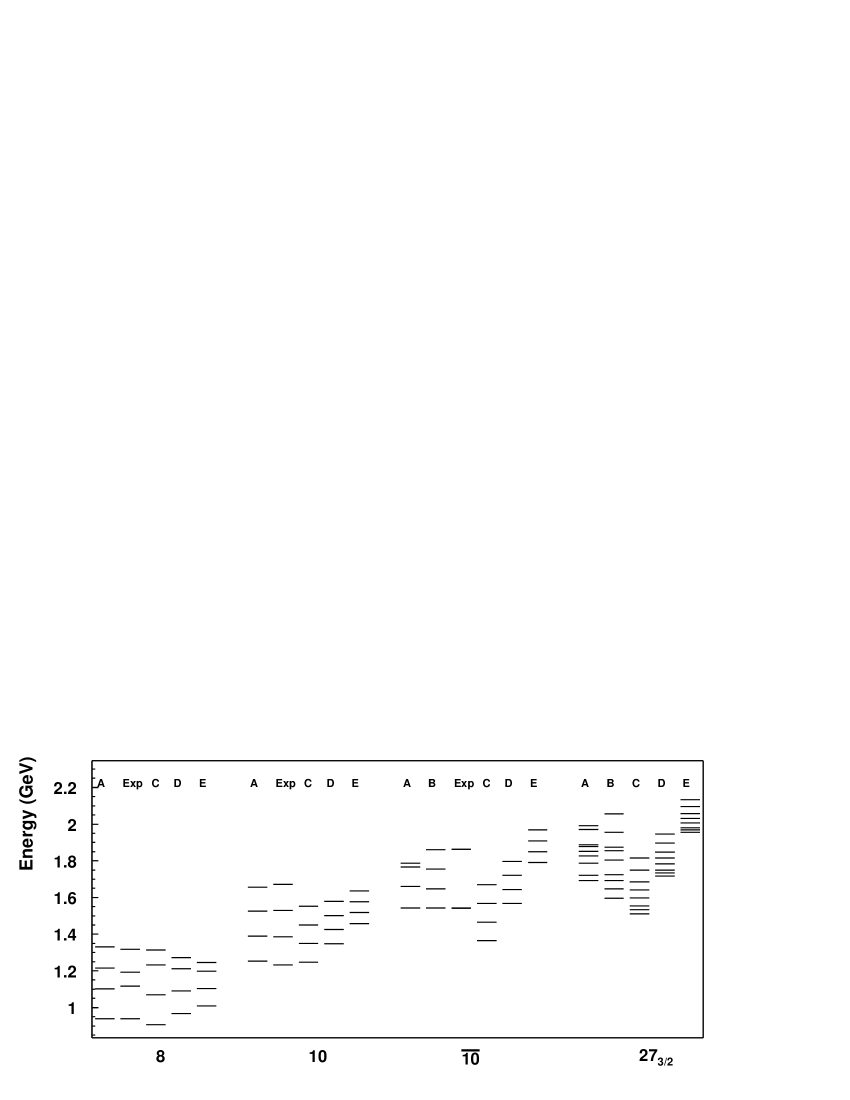
Figure 12: Graphical computation of the 8, 10, $\overline{\bf 10}$ and ${\bf 27}_{3/2}$ mass spectrums. Case A corresponds to the fit A from Fig. 4 in Ref. WK . Case B is Fig. 4 from Ell . Cases C, D and E represents this paper for the fit (iii) and for Skyrme charge $e=4.0;\,4.5;\,5.0$, respectively. For the $\overline{\bf 10}$ experimental masses we use $M^{\rm exp}_{\Theta^{+}}=1540$ MeV and $M^{\rm exp}_{\Xi^{--}_{3/2}}=1861$ MeV.

Comparing the pure Skyrme model prediction for absolute masses of ${\bf 8},{\bf 10}$ and $\overline{\bf 10}$ in Ref. WK (fits A and B in Table 2) with our results for the mass spectrums (for $e=4.0;\,4.1$), presented in Tables 6 and 7, we have found up to 8 % discrapance. One of the reasons is that the fits A and B in Table 2 of Ref. K were obtained for closed but different $e$’s, i.e. for $e=3.96$ and $e=4.12$, respectively. Also, from Tables 6 and 7 one can see that for $e=4.2$, fit (iii), mass spectrum differs from the experiment $\leq 8$% for $\Omega^{-}$, $\Theta^{+}$ and $\Xi_{3/2}^{--}$. Other estimated masses are $\leq\;5$% different from experiment. Comparing our results for ${\bf 27}_{3/2}$ from Table 7, with the Skyrme model prediction of Ref. WK (fits A and B in Figure 4) shows that our case (iii) with $4.3\,\leq\,e\,\leq\,4.7$ supports the fit B, and for $4.4\,\leq\,e\,\leq\,4.6$ agrees nicely with the fit A. Both fits A and B from WK lies between $4.0\,\leq\,e\,\leq\,4.6$ for case (ii). Case (iii) with $4.2\,\leq\,e\,\leq\,4.7$ support also the results presented in Table 1. of Ref. WM . For the narrower $e$-range, $4.4\leq e\leq 4.7$, the prediction for the $\overline{\bf 10}$ masses would lie inside the following range of values $1526\leq\,M_{\Theta^{+}}\,\leq 1654$ MeV, $1607\,\leq M_{\rm N^{*}}\,\leq 1723$ MeV, $1687\,\leq M_{\Sigma_{\overline{10}}}\leq 1792$ MeV and $1768\,\leq\,M_{\Xi^{--}_{3/2}}\,\leq 1861$ MeV, respectively. From Tables 6 and 7 we conclude that in the minimal approach the best fit for 27_3/2-plet mass spectrum, as a function of $e$ and for $f_{K}\not=f_{\pi}$, would lie between $e\simeq 4.2$ and $e\simeq 4.7$, just like for the octet, decuplet and anti-decuplet mass spectrums DT , and agree reasonably well with both baryon spectrums from Table 4.1 in Ref. wei and from Table 2 (fits A and B) of Ref. K , respectively. In Table 7 masses of $\Lambda^{*}$ and $\Xi^{*}_{\frac{3}{2}}$ are equal due to the absence of anomalous moments of inertia MP ; HB in the model used in this paper. Note, however, that anomalous moments of inertia contributions are parametrized in WM ; Ell to be at best $\sim$ 1 % for the $\Xi^{*}_{\frac{3}{2}}$ mass, for example. Clearly, this way, they represent just the fine–tuning type of effects. For a few fixed values of $e$ the mass spectrums of ${\bf 8},{\bf 10}$, $\overline{\bf 10}$ and ${\bf 27}_{3/2}$-plets are given in Figure 12.

The higher SU(3)_f representation mass splittings $\Delta_{i},\,i=3,...,12$, for the multiplets ${\bf 8},{\bf 10},\overline{\bf 10},{\bf 27},\bf{35},\overline{\bf 35}$ and $\bf 64$ expressed in terms of decuplet–octet and antidecuplet–octet mass splittings $\Delta_{1}$ and $\Delta_{2}$ are given in (37) and (39). With the help of Table 8, from (37) we obtain predictions for mass splittings $\Delta_{i},\,i=5,...,12$, as functions of different dynamical assumptions (II.3) and the Skyrme charge $e$. For example for case (iii), and for the range of $4.4\leq\,e\,\leq 4.7$ which fits well the antidecuplet masses, we predict the following range for the mass splittings $536\,\leq\Delta_{2}\,\leq 641$ MeV and $250\,\leq\Delta_{4}\,\leq 301$ MeV, respectively. It is important to stress that, since the mass splittings (37-40) depend on the inverse moments of inertia (29) and (30) only, i.e. there are no additional inputs of the same or higher power in $e$, and consequently they scale as $\Delta^{\cal R^{\prime}}_{\cal R}\sim e^{3}$, the model predicting power for them is the most sensitive. This is illustrated in Figure 12, by the difference between cases C$(e=4)$, D$(e=4.5)$ and E$(e=5)$ for the ${\overline{\bf 10}}$ and ${\bf 27}_{3/2}$ spectrums, where spectral lines follows notations from Tables 6 and 7: $({\bf 8})=({\rm N},\Lambda,\Sigma,\Xi)$, $({\bf 10})=(\Delta,\Sigma^{*},\Xi^{*},\Omega)$, $(\overline{\bf 10})=(\Theta^{+},{\rm N}^{*},\Sigma_{\overline{10}},\Xi^{--}_{3/2})$ and $({\bf 27}_{3/2})=(\Theta_{1},{\rm N}^{*}_{\frac{3}{2}},\Sigma_{2},{\rm N}^{*}_{\frac{1}{2}},\Sigma_{1},\Lambda^{*},\Xi^{*}_{\frac{3}{2}},\Xi^{*}_{\frac{1}{2}},\Omega_{1})$, in accord with notation in Fig. 4 from Ell . Note that in Figure 12 column A, for ${\bf 27}_{3/2}$-plet, (extracted from Fig. 4 column A of WK ) the state $\Xi^{*}_{\frac{3}{2}}\equiv(-1,3/2)$ lies below state $\Sigma_{1}\equiv(0,1)$, due to the absence of the configuration mixing in the evaluation of the ${\bf 27}_{3/2}$-plet spectrum in this paper and in Ref. Ell .

Although we are using simple version of the total action (9), our results for the nucleon axial-vector coupling, moments of inertia, mass spectrum and mass differences given in Tables 4–8, do agree well with the other Skyrme model based estimates MP ; dia1 ; wei1 ; WK ; K ; pra3 ; Itz ; Ell ; wei . Careful inspection of the results for the ${\bf 27}_{3/2}$-plet mass spectrum from Fig. 4 of Ref. WK also shows approximative agreement with our results, $\delta_{1},...,\delta_{8}$, for $4.2\,\leq\,e\,\leq 4.7$ fit (iii), presented in Table 9 and in Figs. 10 and 11. These numbers are in good agreement with the results obtained recently WK ; K ; WM ; Ell ; HW . On top of the importance of the $e$-dependence it turns out that the dependence on the difference between $f_{\pi}$ and $f_{K}$ is crucial for the correct description of the small mass splittings in (37). For the small mass splittings, like $\Delta_{3}$, the contribution of the term proportional to $(f^{2}_{K}-f^{2}_{\pi})$ in the SU(3)_f symmetry breaking term ${\cal L}_{\rm SB}$ plays a major role. It is clear from Figs. 2-11 that SB effects are sizeable and change the relevant quantities. The exception is the $g_{A}$ which change modestly.

The ${\bf 27}_{3/2}$–$\overline{\bf 10}$ mass splittings, given in Tables 8 and 9, are quantities whose measured values, together with measurements of the decay modes branching ratios and relevant widths, would determine the spins 3/2 or 1/2, of observed objects like $\Xi^{--}_{3/2}$, placing it into the right SU(3)_f representation $\overline{\bf 10}$, ${\bf 27}_{3/2}$ or ${\bf 27}_{1/2}$. We do expect that experimental analysis, considering other members of the ${\bf 27}_{3/2}$ and $\overline{\bf 10}$-plets, should be performed in the near future. Since the mass splittings $\Delta_{3}$ represent the smallest splittings among all of the splittings between the SU(3)_f multiplets ${\bf 8}$, ${\bf 10}$, $\overline{\bf 10}$, ${\bf 27}$, ${\bf 35}$, $\overline{\bf 35}$ and ${\bf 64}$ we would urge our colleagues to continue present penta-quark spectral and decay modes experimental analysis and find the penta-quark members of the ${\bf 27}_{3/2}$-plet which would mix with or lie just above the penta-quark family of the $\overline{\bf 10}$-plet. All mentioned experiments would finally show which model, quark or soliton in general, is better describing penta-quark, septu-quark, etc. states. However, one might speculate that the correct description of those states lie somewhere in between.

We hope that the present calculation, taken together with the analogous calculation in wei ; WK ; K ; pra3 ; WM ; Ell ; DT will contribute to understanding of the overall picture of the baryonic mass spectrum and mass splittings in the Skyrme model, as well as for further computations of other non perturbative, dimension-6 operator matrix elements between different baryon states dppt ; dppt1 ; tra ; prat .

We would like to thank T. Antičić and K. Kadija for helpful discussions. One of us (JT) would like to thank V.B. Kopeliovich, A.V. Manohar, M. Praszalowicz and J. Wess for stimulating discussions and Theoretische Physik, Universität München and Theory Division CERN, where part of this work was done, for hospitality. This work was supported by the Ministry of Science and Technology of the Republic of Croatia under Contract 0098002.

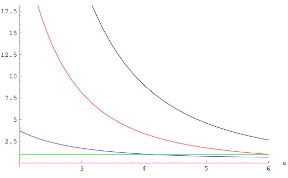
Figure 2: Fit (i): The SB quantity $\gamma$ (pink) in GeV, dimensionles size of soliton $x^{\prime}_{0}$ (green), nucleon axial-vector constant $g_{A}$ (blue), moments of inertia $\lambda_{s}$ (red) in GeV^-1 and $\lambda_{c}$ (black) in GeV^-1.

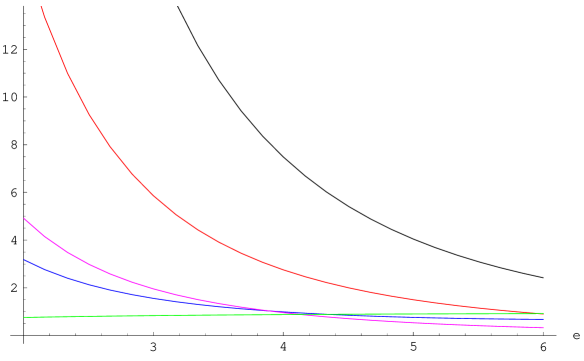
Figure 3: Fit (ii): Dimensionles size of soliton $x^{\prime}_{0}$ (green), nucleon axial-vector constant $g_{A}$ (blue), the SB quantity $\gamma$ (pink) in GeV, moments of inertia $\lambda_{s}$ (red) in GeV^-1 and $\lambda_{c}$ (black) in GeV^-1.

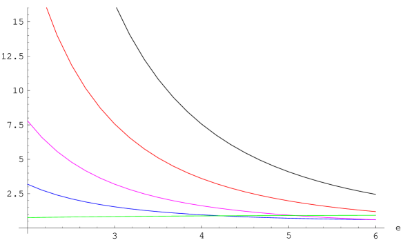
Figure 4: Fit (iii): Dimensionles size of soliton $x^{\prime}_{0}$ (green), nucleon axial-vector constant $g_{A}$ (blue), the SB quantity $\gamma$ (pink) in GeV, moments of inertia $\lambda_{s}$ (red) in GeV^-1 and $\lambda_{c}$ (black) in GeV^-1.

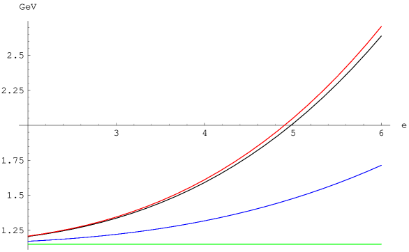
Figure 5: Fit (i): Mass spectrums for 8 (green), 10 (blue), $\overline{\bf 10}$ (black) and ${\bf 27}_{3/2}$ (red).

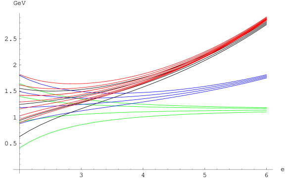
Figure 6: Fit (ii): Mass spectrums for 8 (green), 10 (blue), $\overline{\bf 10}$ (black) and ${\bf 27}_{3/2}$ (red).

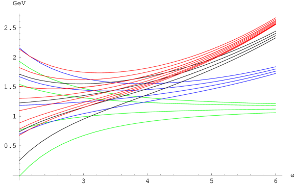
Figure 7: Fit (iii): Mass spectrums for 8 (green), 10 (blue), $\overline{\bf 10}$ (black) and ${\bf 27}_{3/2}$ (red).

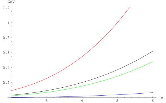
Figure 8: Fit (ii): Mean mass splittings $\Delta_{3}$ (blue), $\Delta_{4}$ (green), $\Delta_{1}$ (black) and $\Delta_{2}$ (red).

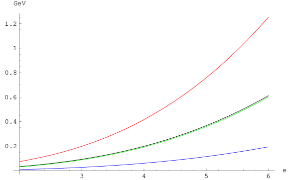
Figure 9: Fit (iii): Mean mass splittings $\Delta_{3}$ (blue), $\Delta_{4}$ (green), $\Delta_{1}$ (black) and $\Delta_{2}$ (red).

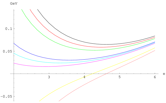
Figure 10: Fit (ii): Mass splittings $\delta_{4,7,2,5,8,6,3,1}$ - brown, yellow, pink, light-blue, dark-blue, green, red and black, respectively.

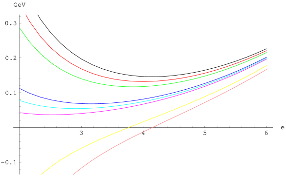
Figure 11: Fit (iii): Mass splittings $\delta_{4,7,2,5,8,6,3,1}$ - brown, yellow, pink, light-blue, dark-blue, green, red and black, respectively.

References

- (1) T. Nakano et al. [LEPS Collaboration], Phys. Rev. Lett. 91, 012002 (2003) [arXiv:hep-ex/0301020].
- (2) V. V. Barmin et al. [DIANA Collaboration], Phys. Atom. Nucl. 66, 1715 (2003) [arXiv:hep-ex/0304040];
- (3) S. Stepanyan et al. [CLAS Collaboration], Phys. Rev. Lett. 91, 252001 (2003) [arXiv:hep-ex/0307018];
- (4) J. Barth et al. [SAPHIR Collaboration], arXiv:hep-ex/0307083.
- (5) A. Aleev et al. [SVD Collaboration], arXiv:hep-ex/0401024.
- (6) C. Alt et al. [NA49 Collaboration], arXiv:hep-ex/0310014.
- (7) L. C. Biedenharn and Y. Dothan, “Monopolar Harmonics In SU(3)-F As Eigenstates Of The Skyrme-Witten Model For Baryons,” published in Y. Ne’eman Festschrift, From SU(3) To Gravity, p.15-34, E. Gotsman, G. Tauber, Eds., (1984), Print-84-1039 (DUKE).
- (8) M. Praszalowicz, TPJU-5-87 Talk presented at the Cracow Workshop on Skyrmions and Anomalies, Mogilany, Poland, Feb 20-24, 1987.
- (9) H. Walliser, Nucl. Phys. A 548 (1992) 649; A. Blotz, D. Diakonov, K. Goeke, N. W. Park, V. Petrov and P. V. Pobylitsa, Nucl. Phys. A 555 (1993) 765.
- (10) N. W. Park, J. Schechter and H. Weigel, Phys. Rev. D 43 (1991) 869.
- (11) D. Diakonov, V. Petrov and M. V. Polyakov, Z. Phys. A 359, 305 (1997) [arXiv:hep-ph/9703373].
- (12) H. Weigel, Eur. Phys. J. A 2, 391 (1998) [arXiv:hep-ph/9804260].
- (13) H. Walliser and V. B. Kopeliovich, J. Exp. Theor. Phys. 97, 433 (2003) [Zh. Eksp. Teor. Fiz. 124, 483 (2003)] [arXiv:hep-ph/0304058].
- (14) V. Kopeliovich, arXiv:hep-ph/0310071; Physics-Uspekhi 74, 309 (2004).
- (15) M. Praszalowicz, Phys. Lett. B 575, 234 (2003) [arXiv:hep-ph/0308114].
- (16) N. Itzhaki, I. R. Klebanov, P. Ouyang and L. Rastelli, arXiv:hep-ph/0309305.
- (17) B. Wu and B. Q. Ma, arXiv:hep-ph/0312041; B. Wu and B. Q. Ma, Phys. Lett. B 586, 62 (2004) [arXiv:hep-ph/0312326].
- (18) J. Ellis, M. Karliner and M. Praszalowicz, arXiv:hep-ph/0401127.
- (19) G. Duplancic and J. Trampetic, arXiv:hep-ph/0402027.
- (20) H. Weigel, hep-ph/0404173.
- (21) G. Duplancic, H. Pasagic and J. Trampetic, hep-ph/0404193.
- (22) S. L. Zhu, Phys. Rev. Lett. 91, 232002 (2003) [arXiv:hep-ph/0307345].
- (23) M. Karliner and H. J. Lipkin, arXiv:hep-ph/0307243.
- (24) L. Y. Glozman, Phys. Lett. B 575, 18 (2003) [arXiv:hep-ph/0308232].
- (25) F. Huang, Z. Y. Zhang, Y. W. Yu and B. S. Zou, arXiv:hep-ph/0310040.
- (26) S. M. Gerasyuta and V. I. Kochkin, arXiv:hep-ph/0310227.
- (27) R. L. Jaffe and F. Wilczek, Phys. Rev. Lett. 91, 232003 (2003) [arXiv:hep-ph/0307341];
- (28) R. Jaffe and F. Wilczek, arXiv:hep-ph/0312369;
- (29) R. Jaffe and F. Wilczek, arXiv:hep-ph/0401034.
- (30) F. Csikor, Z. Fodor, S. D. Katz and T. G. Kovacs, JHEP 0311, 070 (2003) [arXiv:hep-lat/0309090],
- (31) S. Sasaki, arXiv:hep-lat/0310014.
- (32) T. W. Chiu and T. H. Hsieh, arXiv:hep-ph/0403020; arXiv:hep-ph/0404007.
- (33) E. Jenkins and A. V. Manohar, arXiv:hep-ph/0402024.
- (34) D. Diakonov and V. Petrov, arXiv:hep-ph/0310212.
- (35) D. Borisyuk, M. Faber and A. Kobushkin, arXiv:hep-ph/0307370; arXiv:hep-ph/03412213.
- (36) R. Bijker, M. M. Giannini and E. Santopinto, arXiv:hep-ph/0310281.
- (37) D. Diakonov, V. Petrov and M. Polyakov, arXiv:hep-ph/0404212.
- (38) E. Jenkins and A. V. Manohar, arXiv:hep-ph/0401190.
- (39) T.H.R. Skyrme, Proc. Roy. Soc. A260, 127 (1961); Nucl. Phys. 31, 556 (1962); J. Math. Phys. 12, 1735 (1971). For reviews on the Skyrme model, see G. Holzwarth and B. Schwesinger, Rep. Prog. Phys. 49, 82 (1986); I. Zahed and G.E. Brown, Phys. Rep. 142, 481 (1986).
- (40) G. ’t Hooft, Nucl. Phys. B72, 461 (1974); G. Rossi and G. Veneziano, Nucl. Phys. B123, 507 (1977).
- (41) E. Witten, Nucl. Phys. B160, 57 (1979); M. Cvetic and J. Trampetic, Phys. Rev. D 33, 1437 (1986).
- (42) A.P. Balachandran, V.P. Nair, S.G. Rajeev and A. Stern, Phys. Rev. Lett. 49, 1124 (1982); Phys. Rev. D27, 144 (1983);
- (43) E. Witten, Nucl. Phys. B223, 422 (1983) and 433 (1983).
- (44) A.D. Jackson and M. Rho, Phys. Rev. Lett. 51, 751 (1983); M. Rho, A.S. Goldhaber and G.E. Brown, Phys. Rev. Lett. 51, 743 (1983).
- (45) G. Adkins, C.R. Nappi and E. Witten, Nucl. Phys. B228, 552 (1983); G. Adkins and C.R. Nappi, Phys. Lett. 137B, 251 (1984); Nucl. Phys. B233, 109 (1984).
- (46) G. Adkins and C.R. Nappi, Nucl. Phys. B249, 507 (1985).
- (47) E. Guadagnini, Nucl. Phys. B236, 35 (1984); P.O. Mazur, M.A. Nowak and M. Praszaowicz, Phys. Lett. 147B, 137 (1984); A. V. Manohar, Nucl. Phys. B 248, 19 (1984); M. Chemtob, Nucl. Phys. B 256, 600 (1985); M. Sriram, H.S. Mani and R. Ramachandran, Phys. Rev. D30, 1141 (1984); M. Praszaowicz, Phys. Lett. 158B, 264 (1985);
- (48) H. Weigel, Int. J. Mod. Phys. A 11, 2419 (1996) [arXiv:hep-ph/9509398]; J. Schechter and H. Weigel, hep-ph/9907554 (1999).
- (49) J. Wess and B. Zumino, Phys. Lett. 37B, 95 (1971).
- (50) J. Goldstone and F. Wilzcek, Phys. Rev. Lett. 47, 986 (1981); J. Goldstone and R.L. Jaffe, Phys. Rev. Lett. 51, 1518 (1983).
- (51) H.S. Saratchandra and J. Trampetic, Phys. Lett. 144B, 433 (1984).
- (52) H. Yabu and K. Ando, Nucl. Phys. B301, 601 (1988).
- (53) D.I. Diakonov, V.Yu. Petrov and M. Praszaowicz, Nucl. Phys. B323, 53 (1989).
- (54) N. Toyota and K. Fujii, Prog. Theor. Phys. 75, 340 (1986); N. Toyota, Prog. Theor. Phys. 77, 688 (1987); Y. Kondo, S. Saito and T. Otofuji, Phys. Lett. 161B, 1 (1990).
- (55) G. Duplancic, H. Pasagic, M. Praszalowicz and J. Trampetic, Phys. Rev. D 64, 097502 (2001) [arXiv:hep-ph/0104281];
- (56) G. Duplancic, H. Pasagic, M. Praszalowicz and J. Trampetic, Phys. Rev. D 65, 054001 (2002) [arXiv:hep-ph/0109216]; G. Duplancic, H. Pasagic and J. Trampetic, arXiv:hep-ph/0405162.
- (57) J. Trampetic, Phys. Lett. 144B, 250 (1984).
- (58) M. Praszaowicz and J. Trampetic, Phys. Lett. 161B, 169 (1985) and Fizika 18, 391 (1986).
- (59) J.F. Donoghue, H. Golowich and B.R. Holstein, Dynamics of the Standard Model (Cambridge Univ. Press, Cambridge, 1994).
- (60) M. Praszaowicz, Act. Phys. Pol. B22, 523 (1991).
- (61) E. Wigner, Group Theory, Academic Press; H. Weyl, The Theory of Groups and Quantum Mechanics, (Metheun, London, 1931; reissued Dover, New York, 1949); The Classical Groups (Princeton Univ. Press, Princeton, 1946); A.J.G. Hey, in Proceedings of the Topical Conference on Baryon Resonances, Oxford, 1976, edited by R.T. Ross and D.H. Saxon (Rutherford Lab., Chilton, Didcot, England, 1977); B.R. Martin, ibid.
- (62) P. Cvitanovic, Phys. Rev. D14, 1536 (1976).
- (63) Review of Particle Properties, Eur. Phys.J. C15, 1 (2000).
- (64) J.J. de Swart, Rev. Mod. Phys. 35, 916 (1963); P. McNamee, S.J. and F. Chilton, Rev. Mod. Phys. 36, 1005 (1964).
- (65) D. Finkelstein and J. Rubinstein, J. Math. Phys. (NY) 9, 1762 (1968).