Supersymmetric Origin of Neutrino Mass

Abstract

Supersymmetry with breaking of R-parity provides an attractive way to generate neutrino masses and lepton mixing angles in accordance to present neutrino data. We review the main theoretical features of the bilinear R-parity breaking (BRpV) model, and stress that it is the simplest extension of the minimal supersymmetric standard model (MSSM) which includes lepton number violation. We describe how it leads to a successful phenomenological model with hierarchical neutrino masses. In contrast to seesaw models, the BRpV model can be probed at future collider experiments, like the Large Hadron Collider or the Next Linear Collider, since the decay pattern of the lightest supersymmetric particle provides a direct connection with the lepton mixing angles determined by neutrino experiments.

1 Introduction

A combination of solar, atmospheric, reactor and accelerator neutrino experiments fukuda:1998mi , ahmad:2002jz , eguchi:2002dm have now firmly established the existence of neutrino masses and therefore the incompleteness of the standard model of electroweak interactions. The determination of neutrino oscillation parameters presented in Ref. Maltoni:foc uses the most recent data and state-of-the-art solar and atmospheric neutrino fluxes. For previous reviews and references see pakvasa:2003zv , Barger:2003qi , gonzalez-garcia:2002dz , Fogli:2003pz . We have now learned that the atmospheric oscillations involving $\nu_{\mu}\leftrightarrow\nu_{\tau}$ are characterized by a nearly maximal mixing, while the solar neutrino mixing angle is large, but significantly non-maximal. With the recent standard solar model fluxes there is a unique range for the solar mass splitting $\Delta m^{2}{sol}$, determined from the data to be about 30 times smaller than the atmospheric mass splitting $\Delta m^{2}{atm}$.

The discovery of neutrino mass constitutes the only solid hint we currently have of physics beyond the standard model. There are theoretical arguments based on the stability of the gauge hierarchy which suggest the existence of physics at the TeV scale. Supersymmetry nilles:1984ge , haber:1985rc provides an answer to both these issues which fits well with unification and string theory ideas Witten:2002ei .

Prompted by these data there has been a rush of theoretical and phenomenological papers on models of neutrino masses and mixings. The most popular idea is to ascribe neutrino masses to physics at a large mass scale in order to implement some variant of the see-saw mechanism gell-mann:1980vs , yanagida:1979 , schechter:1980gr , mohapatra:1981yp . Broken R-parity supersymmetry provides a theoretically interesting and phenomenologically viable alternative to the origin of neutrino mass and mixing aulakh:1982yn , Ross:1985yg , ellis:1985gi , abada:2001zh , Grossman:1999hc , bednyakov:1998cx , Joshipura:2002fc . Here we focus on the case of supersymmetry with bilinear R-parity breaking diaz:1998xc . This is the simplest of all R parity violating models. It also provides the simplest extension of the MSSM diaz:1998xc to include the violation of lepton number, as well as a calculable framework for neutrino masses and mixing angles in agreement with the experimental data Diaz:2003as , chun:2002vp , hirsch:2000ef , romao:1999up . In this model the atmospheric neutrino mass scale is generated at the tree-level, through the mixing of the three neutrinos with the neutralinos, in an effective ‘low-scale” variant of the seesaw mechanism Ross:1985yg . In contrast, the solar mass and mixings are generated radiatively hirsch:2000ef . BRpV can be considered either as a minimal extension of the MSSM deCampos:1995av , Banks:1995by , deCarlos:1996du , akeroyd:1998iq (with no new particles) valid up to some very high unification energy scale, or as the effective description of a more fundamental theory in which the breaking of R-parity occurs in a spontaneous way by minimizing the scalar potential Masiero:1990uj , romao:1992vu , romao:1997xf .

This short review is mainly devoted to the generation of neutrino masses and lepton mixing, both the tree-level atmospheric neutrino mass scale as well as a description of the main features of the full one-loop calculation of the neutrino-neutralino mass matrix and its various analytic approximations which, in some cases, can be rather simple. For definiteness we will stick to the case of explicit BRpV only.

However, in contrast to the seesaw mechanism, in broken R-parity supersymmetry neutrino masses are generated at the electro-weak scale Diaz:2003as , hirsch:2000ef , romao:1999up . Such low-scale schemes for neutrino masses have the advantage of being testable also outside the realm of neutrino experiments. Although neutrino properties can not be predicted from first principles, their fit to the data allows for unambiguous tests of the theory at accelerator experiments Mukhopadhyaya:1998xj , Allanach:1999bf , romao:1999up , Choi:1999tq , bartl:2000yh , porod:2000hv , restrepo:2001me , hirsch:2002ys , Bartl:2003uq , Hirsch:2003fe . Indeed, the measured lepton mixing angles lead to well defined predictions of the decay properties of the lightest supersymmetric particle (LSP). This is a very general and robust feature of these theories, which holds irrespective of the nature of the LSP. Here we will illustrate possible phenomenological scenarios by discussing some examples of measurements of decay properties of different LSP candidates.

This paper is organized as follows. In Sec. 2 we introduce the main features of the model, discuss the soft supersymmetry breaking terms, as well as the relevant fermion mass matrices and the main features of the corresponding diagonalizing matrices. In Sec. 3 we discuss the generation of the atmospheric neutrino mass scale at the tree–level, while in Sec. 4 we analyse the main features of the one–loop–induced solar neutrino mass scale, including a discussion of the relevant Feynman graph topologies. We also give simplified approximation formula for the solar mixing angle. We then turn briefly to collider phenomenology and how the model under discussion could be tested in LSP decays in Sec. 5 before we conclude and summarize our results in Sec. 6.

2 Formalism

In this section we introduce the main features of the model and the relevant mass matrices. The superpotential of the model and the soft SUSY breaking terms are given, approximate solutions to the tadpole equations discussed.

2.1 The Superpotential and the Soft Breaking Terms

The minimal BRpV model we are working with is characterized by the presence of three extra bilinear terms in the superpotential analogous to the $\mu$ term present in the MSSM. Using the conventions of ref. akeroyd:1998iq it may be given as

$$W=\varepsilon_{ab}\left[h_{U}^{ij}\widehat{Q}_{i}^{a}\widehat{U}_{j}\widehat{H}_{u}^{b}+h_{D}^{ij}\widehat{Q}_{i}^{b}\widehat{D}_{j}\widehat{H}_{d}^{a}+h_{E}^{ij}\widehat{L}_{i}^{b}\widehat{R}_{j}\widehat{H}_{d}^{a}-\mu\widehat{H}_{d}^{a}\widehat{H}_{u}^{b}+\epsilon_{i}\widehat{L}_{i}^{a}\widehat{H}_{u}^{b}\right]$$ (1)

where the first three terms are the usual MSSM Yukawa terms, $\mu$ is the Higgsino mass term of the MSSM, and $\epsilon_{i}$ are the three new terms which violate lepton number in addition to R–Parity. The couplings $h_{U}$, $h_{D}$ and $h_{E}$ are $3\times 3$ Yukawa matrices and $\mu$ and $\epsilon_{i}$ are parameters with units of mass. The smallness of the bilinear term $\epsilon_{i}$ in eq. (1) may arise from a suitable symmetry. In fact any solution to the $\mu$ problem Giudice:1988yz potentially explains also the “$\epsilon_{i}$-problem” nilles:1997ij . A common origin for the $\epsilon_{i}$ terms that account for the neutrino oscillation data, and the $\mu$ term responsible for electroweak symmetry breaking can be ascribed to a horizontal family symmetry of the type suggested in Ref. Mira:2000gg .

The smallness of $\epsilon_{i}$ could also arise dynamically in models with spontaneous breaking of R parity Masiero:1990uj , romao:1992vu , romao:1997xf , where it is given as the product of a Yukawa coupling times a singlet sneutrino vacuum expectation value.

Supersymmetry breaking is parameterized with a set of soft supersymmetry breaking terms. In the MSSM these are given by

$${\cal L}_{soft}^{MSSM} = M_{Q}^{ij2}\widetilde{Q}^{a*}_{i}\widetilde{Q}^{a}_{j}+M_{U}^{ij2}\widetilde{U}_{i}\widetilde{U}^{*}_{j}+M_{D}^{ij2}\widetilde{D}_{i}\widetilde{D}^{*}_{j}+M_{L}^{ij2}\widetilde{L}^{a*}_{i}\widetilde{L}^{a}_{j}+M_{R}^{ij2}\widetilde{R}_{i}\widetilde{R}^{*}_{j}$$

$$\!\!\!\!+m_{H_{d}}^{2}H^{a*}_{d}H^{a}_{d}+m_{H_{u}}^{2}H^{a*}_{u}H^{a}_{u}-\left[{\textstyle{1\over 2}}M_{s}\lambda_{s}\lambda_{s}+{\textstyle{1\over 2}}M\lambda\lambda+{\textstyle{1\over 2}}M^{\prime}\lambda^{\prime}\lambda^{\prime}+h.c.\right]$$

$$\!\!\!\!+\varepsilon_{ab}\left[A_{U}^{ij}\widetilde{Q}_{i}^{a}\widetilde{U}_{j}H_{u}^{b}+A_{D}^{ij}\widetilde{Q}_{i}^{b}\widetilde{D}_{j}H_{d}^{a}+A_{E}^{ij}\widetilde{L}_{i}^{b}\widetilde{R}_{j}H_{d}^{a}-B\mu H_{d}^{a}H_{u}^{b}\right]\,.$$

In addition to the MSSM soft SUSY breaking terms in ${\cal L}_{soft}^{MSSM}$ the BRpV model contains the following extra terms

$$V_{soft}^{BRpV}=-B_{i}\epsilon_{i}\varepsilon_{ab}\widetilde{L}_{i}^{a}H_{u}^{b}\,,$$ (3)

where the $B_{i}$ have units of mass. In what follows, we neglect intergenerational mixing in the soft terms in eq. (2.1).

The electroweak symmetry is broken when the two Higgs doublets $H_{d}$ and $H_{u}$, and the neutral component of the slepton doublets $\widetilde{L}^{1}_{i}$ acquire non–zero vacuum expectation values (vevs). These are calculated via the minimization of the effective potential or, in the diagrammatic method, via the tadpole equations. The full scalar potential at tree level is

$$V_{total}^{0}=\sum_{i}\left|{\partial W\over\partial z_{i}}\right|^{2}+V_{D}+V_{soft}^{MSSM}+V_{soft}^{BRpV}$$ (4)

where $z_{i}$ is any one of the scalar fields in the superpotential in eq. (1), $V_{D}$ are the $D$-terms, and $V_{soft}^{BRpV}$ is given in eq. (3).

The tree level scalar potential contains the following linear terms

$$V_{linear}^{0}=t_{d}^{0}\sigma^{0}_{d}+t_{u}^{0}\sigma^{0}_{u}+t_{1}^{0}\tilde{\nu}^{R}_{1}+t_{2}^{0}\tilde{\nu}^{R}_{2}+t_{3}^{0}\tilde{\nu}^{R}_{3}\,,$$ (5)

where the different $t^{0}$ are the tadpoles at tree level. They are given by

$$t_{d}^{0} = \Big{(}m_{H_{d}}^{2}+\mu^{2}\Big{)}v_{d}+v_{d}D-\mu\Big{(}Bv_{u}+v_{i}\epsilon_{i}\Big{)}$$

$$t_{u}^{0} = -B\mu v_{d}+\Big{(}m_{H_{u}}^{2}+\mu^{2}\Big{)}v_{u}-v_{u}D+v_{i}B_{i}\epsilon_{i}+v_{u}\epsilon^{2}$$

$$t_{1}^{0} = v_{1}D+\epsilon_{1}\Big{(}-\mu v_{d}+v_{u}B_{1}+v_{i}\epsilon_{i}\Big{)}+{\textstyle{1\over 2}}\Big{(}v_{i}M^{2}_{Li1}+M^{2}_{L1i}v_{i}\Big{)}$$ (6)

$$t_{2}^{0} = v_{2}D+\epsilon_{2}\Big{(}-\mu v_{d}+v_{u}B_{2}+v_{i}\epsilon_{i}\Big{)}+{\textstyle{1\over 2}}\Big{(}v_{i}M^{2}_{Li2}+M^{2}_{L2i}v_{i}\Big{)}$$

$$t_{3}^{0} = v_{3}D+\epsilon_{3}\Big{(}-\mu v_{d}+v_{u}B_{3}+v_{i}\epsilon_{i}\Big{)}+{\textstyle{1\over 2}}\Big{(}v_{i}M^{2}_{Li3}+M^{2}_{L3i}v_{i}\Big{)}$$

where we have introduced the notation

$$H_{d}={{H^{0}_{d}}\choose{H^{-}_{d}}}\,,\qquad H_{u}={{H^{+}_{u}}\choose{H^{0}_{u}}}\,,\qquad\widetilde{L}_{i}={{\tilde{L}^{0}_{i}}\choose{\tilde{\ell}^{-}_{i}}}\,,$$ (7)

and shifted the neutral fields with non–zero vevs as

$$H_{d}^{0}\equiv{1\over{\sqrt{2}}}[\sigma^{0}_{d}+v_{d}+i\varphi^{0}_{d}]\,,\quad H_{u}^{0}\equiv{1\over{\sqrt{2}}}[\sigma^{0}_{u}+v_{u}+i\varphi^{0}_{u}]\,,\quad\tilde{L}_{i}^{0}\equiv{1\over{\sqrt{2}}}[\tilde{\nu}^{R}_{i}+v_{i}+i\tilde{\nu}^{I}_{i}]\,.$$ (8)

The five vacuum expectation values can be expressed in spherical coordinates as

$$v_{d} = v\sin\theta_{1}\sin\theta_{2}\sin\theta_{3}\cos\beta$$

$$v_{u} = v\sin\theta_{1}\sin\theta_{2}\sin\theta_{3}\sin\beta$$

$$v_{3} = v\sin\theta_{1}\sin\theta_{2}\cos\theta_{3}$$ (9)

$$v_{2} = v\sin\theta_{1}\cos\theta_{2}$$

$$v_{1} = v\cos\theta_{1}$$

which preserves the MSSM definition $\tan\beta=v_{u}/v_{d}$ with the $W$ boson mass given as $m_{W}^{2}={\textstyle{1\over 4}}g^{2}(v_{d}^{2}+v_{u}^{2}+v_{1}^{2}+v_{2}^{2}+v_{3}^{2})$. We have also defined $D={\textstyle{1\over 8}}(g^{2}+g^{\prime 2})(v_{1}^{2}+v_{2}^{2}+v_{3}^{2}+v_{d}^{2}-v_{u}^{2})$ and $\epsilon^{2}=\epsilon_{1}^{2}+\epsilon_{2}^{2}+\epsilon_{3}^{2}$. A repeated index $i$ in eq. (6) implies summation over $i=1,2,3$. The five tree level tadpoles $t_{\alpha}^{0}$ are equal to zero at the minimum of the tree level potential, and from there one can determine the tree level vacuum expectation values.

2.2 Radiative Breaking of the Electroweak Symmetry

A reliable description of electroweak symmetry breaking and Higgs boson physics in supersymmetry requires the inclusion of radiative corrections. In the BRpV model the full scalar potential at one–loop level, called effective potential, is

$$V_{total}=V_{total}^{0}+V_{RC}$$ (10)

where $V_{total}^{0}$ is given in Eq. (4) and $V_{RC}$ include the quantum corrections. Following Refs. Diaz:2003as , hirsch:2000ef we use the diagrammatic method, incorporating the radiative corrections through the one–loop corrected tadpole equations. The one loop tadpoles are

$$t_{\alpha}=t^{0}_{\alpha}-\delta t^{\overline{DR}}_{\alpha}+T_{\alpha}(Q)=t^{0}_{\alpha}+\widetilde{T}^{\overline{DR}}_{\alpha}(Q)$$ (11)

where $\alpha=d,u,1,2,3$ and $\widetilde{T}^{\overline{DR}}_{\alpha}(Q)\equiv-\delta t^{\overline{MS}}_{\alpha}+T_{\alpha}(Q)$ are the finite one loop tadpoles. At the minimum of the potential we have $t_{\alpha}=0$, and the vevs calculated from these equations are the renormalized vevs.

Neglecting intergenerational mixing in the soft masses, the five tadpole equations can be conveniently written in matrix form as

$$\left[t_{u}^{0},t_{d}^{0},t_{1}^{0},t_{2}^{0},t_{3}^{0}\right]^{T}={\bf{M}^{2}_{tad}}\left[v_{u},v_{d},v_{1},v_{2},v_{3}\right]^{T}$$ (12)

where the matrix ${\bf{M}^{2}_{tad}}$ is given in hirsch:2000ef and depends on the vevs only through the $D$ term defined above.

In the MSSM limit, where $\epsilon_{i}=v_{i}=0$, the angles $\theta_{i}$ are equal to $\pi/2$. In addition to the above MSSM parameters, our model contains nine new parameters, $\epsilon_{i}$, $v_{i}$ and $B_{i}$. Considering we have three tadpole equations one can take either the 3 $B_{i}$ as input and derive the 3 sneutrino vevs or vice versa, such that we have in total just six new parameters (compared to the MSSM).

In order to have approximate solutions for the tree level vevs, consider the following rotation among the $H_{d}$ and lepton superfields:

$${\bf{M^{\prime}}^{2}_{tad}}={\bf R}{\bf{M}^{2}_{tad}}{\bf R^{-1}}$$ (13)

where the rotation ${\bf R}$ can be split as

$${\bf R}=\left[\begin{array}[]{ccccc}c_{3}&0&0&0&-s_{3}\\ 0&1&0&0&0\\ 0&0&1&0&0\\ 0&0&0&1&0\\ s_{3}&0&0&0&c_{3}\\ \end{array}\right]\times\left[\begin{array}[]{ccccc}c_{2}&0&0&-s_{2}&0\\ 0&1&0&0&0\\ 0&0&1&0&0\\ s_{2}&0&0&c_{2}&0\\ 0&0&0&0&1\\ \end{array}\right]\times\left[\begin{array}[]{ccccc}c_{1}&0&-s_{1}&0&0\\ 0&1&0&0&0\\ s_{1}&0&c_{1}&0&0\\ 0&0&0&1&0\\ 0&0&0&0&1\\ \end{array}\right]\,.$$ (14)

where the three angles are defined as

$$c_{1}={{\mu}\over{\mu^{\prime}}}\,,\qquad\,\,s_{1}={{\epsilon_{1}}\over{\mu^{\prime}}}\,,\qquad\,\,\mu^{\prime}=\sqrt{\mu^{2}+\epsilon_{1}^{2}}\,,$$

$$c_{2}={{\mu^{\prime}}\over{\mu^{\prime\prime}}}\,,\qquad\,s_{2}={{\epsilon_{2}}\over{\mu^{\prime\prime}}}\,,\qquad\,\mu^{\prime\prime}=\sqrt{\mu^{\prime 2}+\epsilon_{2}^{2}}\,,$$ (15)

$$c_{3}={{\mu^{\prime\prime}}\over{\mu^{\prime\prime\prime}}}\,,\qquad s_{3}={{\epsilon_{3}}\over{\mu^{\prime\prime\prime}}}\,,\qquad\mu^{\prime\prime\prime}=\sqrt{\mu^{\prime\prime 2}+\epsilon_{3}^{2}}\,.$$

It is clear that this rotation ${\bf R}$ leaves the $D$ term invariant. The rotated vevs are given by

$$\left[v^{\prime}_{u},v^{\prime}_{d},v^{\prime}_{1},v^{\prime}_{2},v^{\prime}_{3}\right]^{T}={\bf{R}}\left[v_{u},v_{d},v_{1},v_{2},v_{3}\right]^{T}\,,$$ (16)

and under the assumption that $v^{\prime}_{1},v^{\prime}_{2},v^{\prime}_{3}\ll v$, these three small vevs have the approximate solution

$$v^{\prime}_{1}\approx-{{\mu\epsilon_{1}}\over{M^{\prime 2}_{L_{1}}+D}}\left[{{m_{H_{d}}^{2}-M_{L_{1}}^{2}}\over{\mu^{\prime}\mu^{\prime\prime\prime}}}v^{\prime}_{d}+{{B_{1}-B}\over{\mu^{\prime}}}v^{\prime}_{u}\right]\,,$$

$$v^{\prime}_{2}\approx-{{\mu^{\prime}\epsilon_{2}}\over{M^{\prime 2}_{L_{2}}+D}}\left[{{m^{\prime 2}_{H_{d}}-M_{L_{2}}^{2}}\over{\mu^{\prime\prime}\mu^{\prime\prime\prime}}}v^{\prime}_{d}+{{B_{2}-B^{\prime}}\over{\mu^{\prime\prime}}}v^{\prime}_{u}\right]\,,$$ (17)

$$v^{\prime}_{3}\approx-{{\mu^{\prime\prime}\epsilon_{3}}\over{M^{\prime 2}_{L_{3}}+D}}\left[{{m^{\prime\prime 2}_{H_{d}}-M_{L_{3}}^{2}}\over{\mu^{\prime\prime\prime 2}}}v^{\prime}_{d}+{{B_{3}-B^{\prime\prime}}\over{\mu^{\prime\prime\prime}}}v^{\prime}_{u}\right]\,,$$

where we have defined the following rotated soft terms:

$$\!\!\!\!\!\!\!\!\!\!\!\!\!\!\!\!\!m^{\prime 2}_{H_{d}}={{m_{H_{d}}^{2}\mu^{2}+M_{L_{1}}^{2}\epsilon_{1}^{2}}\over{\mu^{\prime 2}}}\,,\quad m^{\prime\prime 2}_{H_{d}}={{m^{\prime 2}_{H_{d}}\mu^{\prime 2}+M_{L_{2}}^{2}\epsilon_{2}^{2}}\over{\mu^{\prime\prime 2}}}\,,\quad m^{\prime\prime\prime 2}_{H_{d}}={{m^{\prime\prime 2}_{H_{d}}\mu^{\prime\prime 2}+M_{L_{3}}^{2}\epsilon_{3}^{2}}\over{\mu^{\prime\prime\prime 2}}}\,,$$

$$\!\!\!\!\!\!\!\!\!\!\!\!\!\!\!\!\!B^{\prime}={{B\mu^{2}+B_{1}\epsilon_{1}^{2}}\over{\mu^{\prime 2}}}\,,\qquad\quad\,\,\,B^{\prime\prime}={{B^{\prime}\mu^{\prime 2}+B_{2}\epsilon_{2}^{2}}\over{\mu^{\prime\prime 2}}}\,,\qquad\quad B^{\prime\prime\prime}={{B^{\prime\prime}\mu^{\prime\prime 2}+B_{3}\epsilon_{3}^{2}}\over{\mu^{\prime\prime\prime 2}}}\,,$$ (18)

$$\!\!\!\!\!\!\!\!\!\!\!\!\!\!\!\!\!M^{\prime 2}_{L_{1}}={{m_{H_{d}}^{2}\epsilon_{1}^{2}+M_{L_{1}}^{2}\mu^{2}}\over{\mu^{\prime 2}}}\,,\quad M^{\prime 2}_{L_{2}}={{m^{\prime 2}_{H_{d}}\epsilon_{2}^{2}+M_{L_{2}}^{2}\mu^{\prime 2}}\over{\mu^{\prime\prime 2}}}\,,\quad M^{\prime 2}_{L_{3}}={{m^{\prime\prime 2}_{H_{d}}\epsilon_{3}^{2}+M_{L_{3}}^{2}\mu^{\prime\prime 2}}\over{\mu^{\prime\prime\prime 2}}}\,.$$

As can be seen from eq. (17) the approximation $v^{\prime}_{1},v^{\prime}_{2},v^{\prime}_{3}\ll v$ is justified if either a) $\epsilon_{i}\ll\mu$ and/or b) $(m_{H_{d}}^{2}-M_{L_{i}}^{2})/\mu^{2}\ll 1$ and $(B_{i}-B)/\mu\ll 1$. The latter holds automatically (to some extent) in many models of supersymmetry breaking, as for example in minimal supergravity Ref. diaz:1998xc .

As in the MSSM, the electroweak symmetry is broken because the large value of the top quark mass drives the Higgs mass parameter $m_{H_{U}}^{2}$ to negative values at the weak scale via its RGE Ibanez:1982fr . In the rotated basis, the parameter $\mu^{\prime\prime\prime 2}$ is determined at one loop by

$$\mu^{\prime\prime\prime 2}=-{1\over 2}\left[m_{Z}^{2}-\widetilde{A}_{ZZ}(m_{Z}^{2})\right]+{{\left(m^{\prime\prime\prime 2}_{H_{d}}+\widetilde{T}^{\overline{DR}}_{v^{\prime}_{d}}\,\right)-\left(m_{H_{u}}^{2}+\widetilde{T}^{\overline{DR}}_{v^{\prime}_{u}}\,\right)t^{\prime 2}_{\beta}}\over{t^{\prime 2}_{\beta}-1}}$$ (19)

where $t^{\prime}_{\beta}=v^{\prime}_{u}/v^{\prime}_{d}$ is defined in the rotated basis and is analogous to $\tan\beta$ in eq. (9) defined in the original basis. The finite $\overline{DR}$ Z-boson self energy is $\widetilde{A}_{ZZ}(m_{Z}^{2})$, and the one–loop tadpoles $T^{\overline{DR}}_{v^{\prime}_{d}}$ and $T^{\overline{DR}}_{v^{\prime}_{u}}$ are obtained by applying to the original tadpoles in eq. (11) the rotation $\bf R$ defined in eq. (14). The radiative breaking of the electroweak symmetry is valid in the BRpV model in the usual way: the large value of the top quark Yukawa coupling drives the parameter $m_{H_{U}}^{2}$ to negative values, breaking the symmetry of the scalar potential.

2.3 Neutral fermion mass matrix

Here we consider the tree level structure of the fermion mass matrices in this model. For a more complete discussion of different mass matrices in BRpV see the Appendix of Ref. hirsch:2000ef . In the basis $\psi^{0T}=(-i\lambda^{\prime},-i\lambda^{3},\widetilde{H}_{d}^{1},\widetilde{H}_{u}^{2},\nu_{e},\nu_{\mu},\nu_{\tau})$ the neutral fermion mass matrix ${\mathbb{M}}_{N}$ is given by

$${\mathbb{M}}_{N}=\left[\begin{array}[]{cc}{\cal M}_{\chi^{0}}&m^{T}\cr\vbox to20.0pt{}m&0\cr\end{array}\right]$$ (20)

where

$${\cal M}_{\chi^{0}}\hskip-2.0pt=\hskip-4.0pt\left[\hskip-7.0pt\begin{array}[]{cccc}M_{1}&0&-\frac{1}{2}g^{\prime}v_{d}&\frac{1}{2}g^{\prime}v_{u}\cr\vbox to12.0pt{}0&M_{2}&\frac{1}{2}gv_{d}&-\frac{1}{2}gv_{u}\cr\vbox to12.0pt{}-\frac{1}{2}g^{\prime}v_{d}&\frac{1}{2}gv_{d}&0&-\mu\cr\vbox to12.0pt{}\frac{1}{2}g^{\prime}v_{u}&-\frac{1}{2}gv_{u}&-\mu&0\cr\end{array}\hskip-6.0pt\right]$$ (21)

is the standard MSSM neutralino mass matrix ($M_{2}$ and $M_{1}$ are the SU(2) and U(1) gaugino soft masses) and

$$m=\left[\begin{array}[]{cccc}-\frac{1}{2}g^{\prime}v_{1}&\frac{1}{2}gv_{1}&0&\epsilon_{1}\cr\vbox to18.0pt{}-\frac{1}{2}g^{\prime}v_{2}&\frac{1}{2}gv_{2}&0&\epsilon_{2}\cr\vbox to18.0pt{}-\frac{1}{2}g^{\prime}v_{3}&\frac{1}{2}gv_{3}&0&\epsilon_{3}\cr\end{array}\right]$$ (22)

characterizes the breaking of R-parity. The full $7\times 7$ neutrino/neutralino mass matrix ${\mathbb{M}}_{N}$ is diagonalized as

$${\cal N}^{*}{\mathbb{M}}_{N}{\cal N}^{-1}={\rm diag}(m_{\chi^{0}_{i}},m_{\nu_{j}})$$ (23)

where $(i=1,\cdots,4)$ for the neutralinos, and $(j=1,\cdots,3)$ for the neutrinos.

$${\cal N}^{*}{\bf M}_{F^{0}}{\cal N}^{-1}={\bf M}_{F^{0}}^{\mathrm{d}iag}$$ (24)

and the eigenvectors are given by

$$F^{0}_{i}={\cal N}_{ij}\psi_{j}$$ (25)

using the basis $\psi=(-i\lambda^{\prime},-i\lambda^{3},\widetilde{H}_{d}^{1},\widetilde{H}_{u}^{2},\nu_{e},\nu_{\mu},\nu_{\tau})$. As discussed in more detail below, to a very good approximation, the rotation matrix can be written as

$${\cal N}^{*}\approx\left(\begin{array}[]{cc}N^{*}&N^{*}\xi^{\dagger}\\ -V_{\nu}^{T}\xi&V_{\nu}^{T}\end{array}\right)$$ (26)

Here, $N$ is the rotation matrix that diagonalizes the $4\times 4$ MSSM neutralino mass matrix, $V_{\nu}$ is the rotation matrix that diagonalizes the tree level neutrino $3\times 3$ mass matrix, and $\xi_{ij}\ll 1$ are the relevant small expansion parameters which characterize the violation of R–parity and whose form will be given in Sec. 3.

2.4 Charged fermion mass matrix

The chargino/lepton mass matrix is given by

$${\mathbb{M}_{C}}=\left[\begin{array}[]{ccccc}M_{2}&{\textstyle{1\over{\sqrt{2}}}}gv_{u}&0&0&0\\ \vbox to18.0pt{}{\textstyle{1\over{\sqrt{2}}}}gv_{d}&\mu&-{\textstyle{1\over{\sqrt{2}}}}\left(h_{E}\right)_{11}v_{1}&-{\textstyle{1\over{\sqrt{2}}}}\left(h_{E}\right)_{22}v_{2}&-{\textstyle{1\over{\sqrt{2}}}}\left(h_{E}\right)_{33}v_{3}\\ \vbox to18.0pt{}{\textstyle{1\over{\sqrt{2}}}}gv_{1}&-\epsilon_{1}&{\textstyle{1\over{\sqrt{2}}}}\left(h_{E}\right)_{11}v_{d}&0&0\\ {\textstyle{1\over{\sqrt{2}}}}gv_{2}&-\epsilon_{2}&0&{\textstyle{1\over{\sqrt{2}}}}\left(h_{E}\right)_{22}v_{d}&0\\ {\textstyle{1\over{\sqrt{2}}}}gv_{3}&-\epsilon_{3}&0&0&{\textstyle{1\over{\sqrt{2}}}}\left(h_{E}\right)_{33}v_{d}\end{array}\right]$$ (27)

We note that the chargino sector decouples from the lepton sector in the limit $\epsilon_{i}=v_{i}=0$. As in the MSSM, the chargino mass matrix is diagonalized by two rotation matrices $\mathbb{U}$ and $\mathbb{V}$ defined by

$${\cal U}^{*}\,{\bf M}_{F^{+}}{\cal V}^{-1}={\bf M}_{F^{+}}^{\mathrm{d}iag}$$ (28)

with the eigenvectors satisfying

$$F^{+}_{Ri}={\cal V}_{ij}\psi^{+}_{j}\,,\qquad F^{-}_{Li}={\cal U}_{ij}\psi^{-}_{j}$$ (29)

in the basis $\psi^{+}=(-i\lambda^{+},\widetilde{H}_{2}^{1},e_{R}^{+},\mu_{R}^{+},\tau_{R}^{+})$ and $\psi^{-}=(-i\lambda^{-},\widetilde{H}_{1}^{2},e_{L}^{-},\mu_{L}^{-},\tau_{L}^{-})$, and with the Dirac fermions being

$$F_{i}^{+}=\left(\begin{array}[]{c}F^{+}_{Ri}\\ \\ \overline{F^{-}_{Li}}\end{array}\right)$$ (30)

To first order in the R-Parity violating parameters we have

$${\cal V}\approx\left(\begin{array}[]{cc}V&V\xi^{T}_{R}\\ -V^{\ell}_{R}\xi^{*}_{R}&V^{\ell}_{R}\end{array}\right)\,,\qquad{\cal U}\approx\left(\begin{array}[]{cc}U&U\xi^{\dagger}_{L}\\ -V^{{\ell}*}_{L}\xi_{L}&V^{{\ell}*}_{L}\end{array}\right)$$ (31)

where $V^{{\ell}*}_{L}$ and $V^{\ell}_{R}$ diagonalize the charged lepton mass matrix according to $V^{{\ell}*}_{L}{\bf M}^{\ell}V^{\ell\dagger}_{R}={\bf M}^{\ell}_{\mathrm{d}iag}$. For most purposes it is sufficient to take $\xi_{R}={\bf 0}_{2\times 3}$, since it is smaller than $\xi_{L}$ typically by a factor of $m_{l}/m_{SUSY}$. Note, that we can choose $V^{{\ell}*}_{L}=V^{\ell\dagger}_{R}={\bf 1}_{3\times 3}$. We then have

$$\xi_{L}^{i1}=a^{L}_{1}\Lambda_{i}\,,\qquad\xi_{L}^{i2}=a^{L}_{2}\Lambda_{i}+b\epsilon_{i}$$ (32)

and

$$a_{1}^{L}={g\over{\sqrt{2}\Delta_{+}}}\,,\qquad a_{2}^{L}=-{{g^{2}v_{u}}\over{2\mu\Delta_{+}}}$$ (33)

where $\Delta_{+}$ is the determinant of the $2\times 2$ chargino mass matrix and

$$\Lambda_{i}=\mu v_{i}+v_{d}\epsilon_{i}\propto v^{\prime}_{i}$$ (34)

are the alignment parameters.

3 Tree–level neutrino mass: the atmospheric scale

The tree-level contribution to neutrino masses from broken R parity supersymmetry has a long history santamaria:1987uq . Thanks to the Super-K findings fukuda:1998mi we will be interested only in the case where the neutrino mass which is determined at the tree level is small, in order to account for the atmospheric neutrino data. The above form for ${\mathbb{M}}_{N}$ is especially convenient in this case in order to provide an approximate analytical discussion valid in the limit of small $R_{p}/\;\>$ violation parameters. Indeed in this case we perform a perturbative diagonalization of the neutral mass matrix, defining

$$\xi=m\cdot{\cal M}_{\chi^{0}}^{-1}$$ (35)

Since the effective RpV parameters are smaller than the weak scale, we can work in a perturbative expansion defined by $\xi\ll 1$, where $\xi$ denotes a $3\times 4$ matrix given as Hirsch:1998kc

$$\xi_{i1} = \frac{g^{\prime}M_{2}\mu}{2det({\cal M}_{\chi^{0}})}\Lambda_{i}$$ (36)

$$\vbox to20.0pt{}\xi_{i2} = -\frac{gM_{1}\mu}{2det({\cal M}_{\chi^{0}})}\Lambda_{i}$$ (37)

$$\vbox to20.0pt{}\xi_{i3} = -\frac{\epsilon_{i}}{\mu}+\frac{(g^{2}M_{1}+{g^{\prime}}^{2}M_{2})v_{u}}{4det({\cal M}_{\chi^{0}})}\Lambda_{i}$$ (38)

$$\vbox to20.0pt{}\xi_{i4} = -\frac{(g^{2}M_{1}+{g^{\prime}}^{2}M_{2})v_{d}}{4det({\cal M}_{\chi^{0}})}\Lambda_{i}$$ (39)

From Eq. (39) and Eq. (34) one can see that $\xi=0$ in the MSSM limit where $\epsilon_{i}=0$, $v_{i}=0$.

If the elements of this matrix satisfy

$$\forall\xi_{ij}\ll 1$$ (40)

then one can use it as expansion parameter in order to find an approximate solution for the mixing matrix ${\cal N}$.

In leading order in $\xi$ the mixing matrix ${\cal N}$ is given by,

$${\cal N}^{*}\hskip-2.0pt=\hskip-2.0pt\left(\hskip-1.0pt\begin{array}[]{cc}N^{*}&0\\ 0&V_{\nu}^{T}\end{array}\hskip-1.0pt\right)\left(\hskip-1.0pt\begin{array}[]{cc}1-{1\over 2}\xi^{\dagger}\xi&\xi^{\dagger}\\ -\xi&1-{1\over 2}\xi\xi^{\dagger}\end{array}\hskip-1.0pt\right)$$ (41)

The second matrix above block-diagonalizes the mass matrix ${\mathbb{M}}_{N}$ approximately to the form diag(${\cal M}_{\chi^{0}},m_{eff}$), where

$$m_{eff} = -m\cdot{\cal M}_{\chi^{0}}^{-1}m^{T}$$ (42)

$$\hskip-8.53581pt=\hskip-8.53581pt \frac{M_{1}g^{2}\!+\!M_{2}{g^{\prime}}^{2}}{4\,det({\cal M}_{\chi^{0}})}\left(\hskip-5.69054pt\begin{array}[]{ccc}\Lambda_{e}^{2}\hskip-1.0pt&\hskip-1.0pt\Lambda_{e}\Lambda_{\mu}\hskip-1.0pt&\hskip-1.0pt\Lambda_{e}\Lambda_{\tau}\\ \Lambda_{e}\Lambda_{\mu}\hskip-1.0pt&\hskip-1.0pt\Lambda_{\mu}^{2}\hskip-1.0pt&\hskip-1.0pt\Lambda_{\mu}\Lambda_{\tau}\\ \Lambda_{e}\Lambda_{\tau}\hskip-1.0pt&\hskip-1.0pt\Lambda_{\mu}\Lambda_{\tau}\hskip-1.0pt&\hskip-1.0pt\Lambda_{\tau}^{2}\end{array}\hskip-8.53581pt\right)$$ (46)

The sub-matrices $N$ and $V_{\nu}$ diagonalize ${\cal M}_{\chi^{0}}$ and $m_{eff}$

$$N^{*}{\cal M}_{\chi^{0}}N^{\dagger}={\rm diag}(m_{\chi^{0}_{i}}),$$ (47)

$$V_{\nu}^{T}m_{eff}V_{\nu}={\rm diag}(0,0,m_{\nu}),$$ (48)

where

$$m_{\nu}=Tr(m_{eff})=\frac{M_{1}g^{2}+M_{2}{g^{\prime}}^{2}}{4\,det({\cal M}_{\chi^{0}})}|{\vec{\Lambda}}|^{2}.$$ (49)

The special form of the neutralino/neutrino mass matrix implies that the effective neutrino mass matrix $m_{eff}$ generated after diagonalizing out the heavy neutralinos has a projective form, a feature common to many spontaneous R–parity violating models santamaria:1987uq . This implies that only one neutrino acquires a tree level mass, the other two remaining massless santamaria:1987uq . As a result at the tree approximation one can rotate away one of the three angles in the matrix $V_{\nu}$, leading to

$$V_{\nu}=\left(\begin{array}[]{ccc}1&0&0\\ 0&\cos\theta_{23}&-\sin\theta_{23}\\ 0&\sin\theta_{23}&\cos\theta_{23}\end{array}\right)\times\left(\begin{array}[]{ccc}\cos\theta_{13}&0&-\sin\theta_{13}\\ 0&1&0\\ \sin\theta_{13}&0&\cos\theta_{13}\end{array}\right),$$ (50)

where the mixing angles can be expressed in terms of the alignment vector ${\vec{\Lambda}}$ as follows:

$$\tan\theta_{13}=-\frac{\Lambda_{e}}{(\Lambda_{\mu}^{2}+\Lambda_{\tau}^{2})^{\frac{1}{2}}},$$ (51)

$$\tan\theta_{23}=-\frac{\Lambda_{\mu}}{\Lambda_{\tau}}.$$ (52)

The non-zero tree–level eigenvalue of the neutrino mass matrix is identified with the atmospheric mass scale.

Figure 1: $\Delta m^{2}_{atm}$ versus the BRpV alignment parameters

The calculated $\Delta m^{2}_{atm}$ can be expressed as a function of the alignment parameter ${\vec{\Lambda}}$ (left in Fig. 1), or as function of $|{\vec{\Lambda}}|/(\sqrt{M_{2}}\mu)$ (right in Fig. 1), all of these expressed in GeV. The figure shows that Eq. (49) can be used to fix the relative size of R-parity breaking parameters to obtain the correct $\Delta m^{2}_{atm}$. On the other hand, as shown in Fig  2 the atmospheric angle can be expressed in terms of $\Lambda_{\mu}/\Lambda_{\tau}$. Its maximality is obtained for $\Lambda_{\mu}\simeq\Lambda_{\tau}$ if $\Lambda_{e}$ is smaller than the other two.

Figure 2: The atmospheric angle versus the ratio of BRpV parameters $|\Lambda_{\mu}/\Lambda_{\tau}|$

Let us stress once again that there is no solar mass splitting in the tree approximation so that, as a result, the “solar angle” is not defined, as it can be rotated away by redefining the two degenerate neutrinos schechter:1980gr .

4 One–loop–induced neutrino mass: the solar scale

As we just saw in the BRpV model the atmospheric mass scale and mixing arises at the tree-level. We now discuss the determination of solar neutrino masses and mixings, which are both generated radiatively. One-loop corrections to the neutrino masses can be calculated numerically hirsch:2000ef or analytically Diaz:2003as . While the numerical approach can give “exact” results (exact in the sense of being correct up to higher order effects), the analytic approach, while being less accurate, gives a better understanding about which parameters control the loops and thus the solar neutrino mass and angles in our model. The discussion will therefore mainly concentrate on the analytical calculations.

In principle, in order to find the correct neutrino mixing angles one has to diagonalize the one–loop corrected neutralino/neutrino mass matrix. We define

$$M^{\rm pole}_{ij}=M^{\rm\overline{DR}}_{ij}(Q)+\Delta M_{ij}$$ (53)

where $M^{\rm\overline{DR}}_{ij}(Q)$ is the tree-level pole mass and ${\rm\overline{DR}}$ indicates the dimensional reduction scheme we used in the numerical calculation. One-loop corrections are

$$\Delta M_{ij}={\textstyle{1\over 2}}\left[\widetilde{\Pi}^{V}_{ij}(m_{i}^{2})+\widetilde{\Pi}^{V}_{ij}(m_{j}^{2})\right]-{\textstyle{1\over 2}}\left[m_{\chi^{0}_{i}}\widetilde{\Sigma}^{V}_{ij}(m_{i}^{2})+m_{\chi^{0}_{j}}\widetilde{\Sigma}^{V}_{ij}(m_{j}^{2})\right]\,,$$ (54)

where the symmetrization is necessary to achieve gauge invariance and consistency with the Pauli principle. Here $\widetilde{\Pi}^{V}$ and $\widetilde{\Sigma}^{V}$ are the renormalized self-energies. They contain products of couplings and the usual Passarino-Veltman functions passarino:1979jh .

Diagonalizing the tree-level neutrino mass matrix first and adding then the one-loop corrections before re-diagonalization one finds that the resulting neutrino/neutralino mass matrix has non-zero entries in the neutrino/neutrino, the neutrino/neutralino and in the neutralino/neutralino sectors. We have found Diaz:2003as that the most important part of the one-loop neutrino masses derives from the neutrino/neutrino sector and that the one-loop induced neutrino/neutralino mixing is usually negligible.

The relevant topologies for the one loop calculation of neutrino masses are then illustrated in Fig.3.

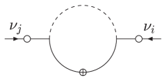
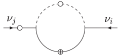
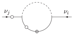
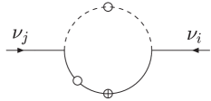
Figure 3: Topologies for neutrino self-energies in the BRpV supersymmetric model

Here our conventions are as follows: open circles with a cross inside indicate genuine mass insertions which flip chirality. On the other hand open circles without a cross correspond to small R-Parity violating projections, indicating how much of an Rp-even/odd mass eigenstate is present in a given Rp-odd/even weak eigenstate. In the actual numerical calculation these projections really belong to the coupling matrices attached to the vertices. However, given the smallness of Rp-violating effects, the pre-diagonalization “insertion-method” proves to be a rather useful tool to develop an analytical perturbative expansion and to acquire a simple understanding of the results.

These topologies have then to be “filled” with all relevant combinations of particles/sparticles. Here we will concentrate on discussing the loop involving bottom/sbottom quarks, since a) it is in large parts of parameter space the numerically most important one. And b) other loops can be calculated in a very similar way Diaz:2003as , although they are more complicated.

The relevant Feynman rules for the bottom-sbottom loops are, in the case of left sbottoms:

with

$$O^{bn\tilde{b}}_{Lij} = -R^{\tilde{b}}_{j1}h_{b}{\cal N}^{*}_{i3}-R^{\tilde{b}}_{j2}{{2g}\over{3\sqrt{2}}}\tan\theta_{W}{\cal N}^{*}_{i1}$$

$$O^{bn\tilde{b}}_{Rij} = R^{\tilde{b}}_{j1}{g\over{\sqrt{2}}}\left({\cal N}_{i2}-{\textstyle{1\over 3}}\tan\theta_{W}{\cal N}_{i1}\right)-R^{\tilde{b}}_{j2}h_{b}{\cal N}^{*}_{i3}$$ (55)

After approximating the rotation matrix ${\cal N}$ we find that expressions with the replacement ${\cal N}\to{\mathrm{N}}$ are valid when the neutral fermion is a neutralino. When the neutral fermion $F^{0}$ is a neutrino, the following expressions hold

$$O^{bn\tilde{b}}_{Lij} \approx R^{\tilde{b}}_{j1}h_{b}\left(a_{3}|\vec{\Lambda}|\delta_{i^{\prime}3}+b\tilde{\epsilon}_{i^{\prime}}\right)+R^{\tilde{b}}_{j2}{{2g}\over{3\sqrt{2}}}\tan\theta_{W}a_{1}|\vec{\Lambda}|\delta_{i^{\prime}3}$$

$$O^{bn\tilde{b}}_{Rij} \approx R^{\tilde{b}}_{j1}{g\over{\sqrt{2}}}\left({\textstyle{1\over 3}}\tan\theta_{W}a_{1}-a_{2}\right)|\vec{\Lambda}|\delta_{i^{\prime}3}+R^{\tilde{b}}_{j2}h_{b}\left(a_{3}|\vec{\Lambda}|\delta_{i^{\prime}3}+b\tilde{\epsilon}_{i^{\prime}}\right)$$ (56)

where $i^{\prime}=i-4$ label one of the neutrinos. $R^{\tilde{b}}_{jk}$ are the rotation matrices connecting weak and mass eigenstate basis for the scalar bottom quarks. In case of no intergenerational mixing in the squark sector $R^{\tilde{b}}_{jk}$ can be parameterized by just one diagonalizing angle $\theta_{\tilde{b}}$.

Putting these couplings together one finds the simplest contribution to the radiatively induced neutrino mass from loops involving bottom quarks and squarks hirsch:2000ef

$$\widetilde{\Pi}_{ij}(0)=-{{N_{c}}\over{16\pi^{2}}}\sum_{r}\left(O^{bn\tilde{b}}_{Rjr}O^{bn\tilde{b}}_{Lir}+O^{bn\tilde{b}}_{Ljr}O^{bn\tilde{b}}_{Rir}\right)m_{b}B_{0}(0,m_{b}^{2},m_{r}^{2})$$ (57)

where $B_{0}(0,m_{b}^{2},m_{r}^{2})$ is a Passarino-Veltman function passarino:1979jh can be written as follows

$$\widetilde{\Pi}_{ij} = -{{N_{c}m_{b}}\over{16\pi^{2}}}2s_{\tilde{b}}c_{\tilde{b}}h_{b}^{2}\Delta B_{0}^{\tilde{b}_{1}\tilde{b}_{2}}\times$$

$$\Big{(}{{\tilde{\epsilon}_{i}\tilde{\epsilon}_{j}}\over{\mu^{2}}}+a_{3}b\left(\tilde{\epsilon}_{i}\delta_{j3}+\tilde{\epsilon}_{j}\delta_{i3}\right)|\vec{\Lambda}|+\left(a_{3}^{2}+\frac{a_{L}a_{R}}{h^{2}_{b}}\right)\delta_{i3}\delta_{j3}|\vec{\Lambda}|^{2}\Big{)}$$

This expression is proportional to the difference of two $B_{0}$ functions,

$$\Delta B_{0}^{\tilde{b}_{1}\tilde{b}_{2}}=B_{0}(0,m_{b}^{2},m_{\tilde{b}_{1}}^{2})-B_{0}(0,m_{b}^{2},m_{\tilde{b}_{2}}^{2})$$ (59)

Parameters $\Lambda_{i}$ have been defined above. The $\tilde{\epsilon}$ parameters are defined as $\tilde{\epsilon}_{i}=\left(V_{\nu}^{T}\right)^{ij}\epsilon_{j}$, and are given by

$$\tilde{\epsilon}_{1} = {{\epsilon_{e}(\Lambda_{\mu}^{2}+\Lambda_{\tau}^{2})-\Lambda_{e}(\Lambda_{\mu}\epsilon_{\mu}+\Lambda_{\tau}\epsilon_{\tau})}\over{\sqrt{\Lambda_{\mu}^{2}+\Lambda_{\tau}^{2}}\sqrt{\Lambda_{e}^{2}+\Lambda_{\mu}^{2}+\Lambda_{\tau}^{2}}}}$$

$$\tilde{\epsilon}_{2} = {{\Lambda_{\tau}\epsilon_{\mu}-\Lambda_{\mu}\epsilon_{\tau}}\over{\sqrt{\Lambda_{\mu}^{2}+\Lambda_{\tau}^{2}}}}$$ (60)

$$\tilde{\epsilon}_{3} = {{\vec{\Lambda}\cdot\vec{\epsilon}}\over{\sqrt{\Lambda_{e}^{2}+\Lambda_{\mu}^{2}+\Lambda_{\tau}^{2}}}}$$

On the other hand $a_{L,R}$ are defined as

$$a_{R}={g\over{\sqrt{2}}}\left({1\over 3}t_{W}a_{1}-a_{2}\right)\,,\qquad a_{L}={g\over{\sqrt{2}}}\,{2\over 3}t_{W}a_{1}$$ (61)

The different terms in eq. (4) can be understood as coming from the graphs corresponding to the first topology of Fig. 3. They have been depicted in more detail in Fig. 4,

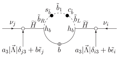
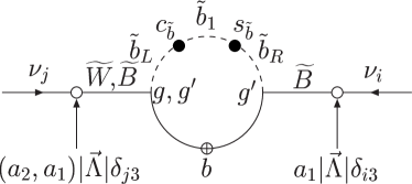
Figure 4: Bottom–Sbottom diagrams for solar neutrino mass in the BRpV model

where we have adopted the following conventions: a) as before, open circles correspond to small R-parity violating projections, indicating how much of a weak eigenstate is present in a given mass eigenstate, (b) full circles correspond to R-parity conserving projections and (c) open circles with a cross inside indicate genuine mass insertions which flip chirality.

The open and full circles should really appear at the vertices since the particles propagating in the loop are the mass eigenstates. We have however separated them to better identify the origin of the various terms. There is another set of graphs analogous to the previous ones which corresponds to the heavy sbottom. They are obtained from the previous graphs making the replacement $\tilde{b}_{1}\to\tilde{b}_{2}$, $s_{\tilde{b}}\to c_{\tilde{b}}$ and $c_{\tilde{b}}\to-s_{\tilde{b}}$. Note that for all contributions to the $2\times 2$ sub-matrix corresponding to the light neutrinos the divergence from $B_{0}(0,m_{b}^{2},m_{\tilde{b}_{1}}^{2})$ is canceled by the divergence from $B_{0}(0,m_{b}^{2},m_{\tilde{b}_{2}}^{2})$, making finite the contribution from bottom-sbottom loops to this sub-matrix, as it should be, since the mass is fully “calculable”.

The second most important contribution to the radiatively induced neutrino mass usually comes from charged-scalar/charged-fermion loops hirsch:2000ef . Since all possible topologies of Fig. (3) contribute to this loop the structure of the contribution from charged Higgs/slepton loops is more complex than that of the bottom-sbottom loop considered above. However, the same topology as for the sbottom/bottom loop also contributes to the charged scalar loop. It leads to a final expression similar to eq. (4), with appropriate replacements, which is good enough for an order-of-magnitude estimate of the charged scalar loop.

4.1 Results for the solar mass scale

We give a discussion of the analytical versus numerical results of the solar mass scale first. In Fig. (5) we show a comparison of approximate and exact calculation for two different numerical data sets. In both figures we show the ratio of the approximate-over-exact solar neutrino mass parameter $m_{\nu_{2}}^{Appr}/m_{\nu_{2}}^{exact}$ versus $\Delta m^{2}{sol}$ in eV², where $m_{\nu_{2}}^{Appr}$ is the approximate loop calculation involving the bottom-sbottom and the charged scalar loop, while $m_{\nu_{2}}^{exact}$ is the exact numerical computation taking into account all loops. The set to the left called “Ntrl” contains neutralinos being the LSP, while the set to the right (Stau) has the charged scalar tau as LSP.

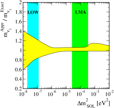
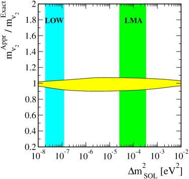
Figure 5: ($m_{\nu_{2}}^{Appr}/m_{\nu_{2}}^{exact}$) versus $\Delta m^{2}{sol}$ [$eV^{2}$] for the set Ntrl (left) and the set Stau (right). $m_{\nu_{2}}^{Appr}$ is the sum of the bottom-sbottom and charged scalar loops, while $m_{\nu_{2}}^{exact}$ is the numerical result for all loops. In case of LMA the approximation works always better than 10 %.

We have found numerically that the terms proportional to ${\tilde{\epsilon}_{i}}\times{\tilde{\epsilon}_{j}}$ in the self energies in Eq. (4) give the most important contribution to $m_{\nu_{2}}$ in the bottom-sbottom loop calculation in most points of our sets. If these terms are dominant one can find a very simple approximation for the bottom-sbottom loop contribution to $m_{\nu_{2}}$. It is given by

$$m_{\nu_{2}}\simeq\frac{3}{16\pi^{2}}\sin(2\theta_{\tilde{b}})m_{b}\Delta B_{0}^{\tilde{b}_{2}\tilde{b}_{1}}\ \frac{({\tilde{\epsilon}}_{1}^{2}+{\tilde{\epsilon}}_{2}^{2})}{\mu^{2}}.$$ (62)

Eq. (62) works surprisingly well for almost all points in our data sets.

The more complicated structure of the charged scalar loop makes it difficult to give a simple equation for $m_{\nu_{2}}$ similar to Eq. (62) for the bottom-sbottom loop. However, we note that Eq. (62), with appropriate replacements, allows us to estimate the typical contributions to the charged scalar loop within a factor of $\sim 3$. However, such an estimate will be biased toward too small or too large $m_{\nu_{2}}$ depending mainly on which SUSY particle is the LSP Diaz:2003as .

4.2 Analytical approximation for the solar mixing angle

In the basis where the tree-level neutrino mass matrix is diagonal the mass matrix at one–loop level can be written as

$$\widetilde{m}_{\nu}=V_{\nu}^{(0)T}m_{\nu}V_{\nu}^{(0)}=\left(\begin{array}[]{ccc}c_{1}\widetilde{\epsilon}_{1}\widetilde{\epsilon}_{1}&c_{1}\widetilde{\epsilon}_{1}\widetilde{\epsilon}_{2}&c_{1}\widetilde{\epsilon}_{1}\widetilde{\epsilon}_{3}\\ c_{1}\widetilde{\epsilon}_{2}\widetilde{\epsilon}_{1}&c_{1}\widetilde{\epsilon}_{2}\widetilde{\epsilon}_{2}&c_{1}\widetilde{\epsilon}_{2}\widetilde{\epsilon}_{3}\\ c_{1}\widetilde{\epsilon}_{3}\widetilde{\epsilon}_{1}&c_{1}\widetilde{\epsilon}_{3}\widetilde{\epsilon}_{2}&c_{0}|\vec{\Lambda}|^{2}+c_{1}\widetilde{\epsilon}_{3}\widetilde{\epsilon}_{3}\end{array}\right)+\cdots$$ (66)

where the $\widetilde{\epsilon}_{i}$ were defined before in Eq. (4). Coefficients $c_{0}$ and $c_{1}$ contain couplings and supersymmetric masses. Since they cancel in the final expression for the angle their exact definition is not necessary in the following. Dots stand for other terms which we will assume to be less important in the following. This matrix can be diagonalized approximately taking in account that

$$x\equiv\frac{c_{1}|\vec{\widetilde{\epsilon}}|^{2}}{c_{0}|\vec{\Lambda}|^{2}}\ll 1$$ (67)

Then

$$\widetilde{m}_{\nu}=c_{0}|\vec{\Lambda}|^{2}\left(\begin{array}[]{ccc}\displaystyle x\,\frac{\widetilde{\epsilon}_{1}\widetilde{\epsilon}_{1}}{|\vec{\widetilde{\epsilon}|^{2}}}&\displaystyle x\,\frac{\widetilde{\epsilon}_{1}\widetilde{\epsilon}_{2}}{|\vec{\widetilde{\epsilon}|^{2}}}&\displaystyle x\,\frac{\widetilde{\epsilon}_{1}\widetilde{\epsilon}_{3}}{|\vec{\widetilde{\epsilon}|^{2}}}\\[11.38109pt] \displaystyle x\,\frac{\widetilde{\epsilon}_{2}\widetilde{\epsilon}_{1}}{|\vec{\widetilde{\epsilon}|^{2}}}&\displaystyle x\,\frac{\widetilde{\epsilon}_{2}\widetilde{\epsilon}_{2}}{|\vec{\widetilde{\epsilon}|^{2}}}&\displaystyle x\,\frac{\widetilde{\epsilon}_{2}\widetilde{\epsilon}_{3}}{|\vec{\widetilde{\epsilon}|^{2}}}\\[11.38109pt] \displaystyle x\,\frac{\widetilde{\epsilon}_{3}\widetilde{\epsilon}_{1}}{|\vec{\widetilde{\epsilon}|^{2}}}&\displaystyle x\,\frac{\widetilde{\epsilon}_{3}\widetilde{\epsilon}_{2}}{|\vec{\widetilde{\epsilon}|^{2}}}&\displaystyle 1+x\,\frac{\widetilde{\epsilon}_{3}\widetilde{\epsilon}_{3}}{|\vec{\widetilde{\epsilon}|^{2}}}\end{array}\right)$$ (71)

The rotation matrix that diagonalizes $\widetilde{m}_{\nu}$ in Eq. (71) can be written as

$$\widetilde{V}_{\nu}^{T}\widetilde{m}_{\nu}\widetilde{V}_{\nu}=\hbox{diag}(m_{1},m_{2},m_{3})$$ (72)

where

$$\widetilde{V}_{\nu}^{T}=\left(\begin{array}[]{ccc}e_{1,1}&e_{1,2}&e_{1,3}\\ e_{2,1}&e_{2,2}&e_{2,3}\\ e_{3,1}&e_{3,2}&e_{3,3}\end{array}\right)$$ (76)

The lepton mixing matrix is then given by

$$U=\left(V_{\nu}^{T}\widetilde{V}_{\nu}^{T}\right)^{T}$$ (77)

The expression for the solar mixing angle can be obtained from:

$$\tan^{2}\theta{sol}=\frac{U_{e2}^{2}}{U_{e1}^{2}}$$ (78)

From the above equations we obtain the very simple expression for the solar mixing angle,

$$\tan^{2}\theta{sol}=\frac{\widetilde{\epsilon}_{1}^{2}}{\widetilde{\epsilon}_{2}^{2}}$$ (79)

This formula is a very good approximation if the one–loop matrix has the structure $\epsilon_{i}\times\epsilon_{j}$, as is the case of the bottom-sbottom loop if $m_{\nu_{3}}\gg m_{\nu_{2}}$, as illustrated in Fig. 6.

In the left panel we show a calculation comparing for all points the approximate to the exact solar angle in the set with neutralino LSP, while the right panel shows a subset of points with the cut $\sin(2\theta_{\tilde{b}})\Delta B_{0}^{\tilde{\tau}_{2}\tilde{\tau}_{1}}>0.02$. Note that this cut is designed so as to favor points in which there is a sizeable bottom-sbottom loop contribution to the full one-loop neutrino mass. One sees from the right panel that for this case the true solar angle is well approximated by our analytical formula. Note finally that eq. (79) will fail completely, if $\Lambda_{\mu}\equiv\Lambda_{\tau}$ and $\epsilon_{\mu}\equiv\epsilon_{\tau}$, since then ${\widetilde{\epsilon}_{2}^{2}}=0$, see Eq. (4). This is the origin of the “sign condition” discussed in hirsch:2000ef .

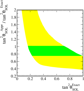
Figure 6: (${\tan^{2}\theta{sol}}^{Appr}/{\tan^{2}\theta{sol}}^{exact}$) versus ${\tan^{2}\theta{sol}}^{exact}$. On the left panel the darker region contains over 90% of the points in our sample. In the right panel the points in the region shown satisfy the cut $\sin(2\theta_{\tilde{b}})\Delta B_{0}^{\tilde{\tau}_{2}\tilde{\tau}_{1}}>0.02$ .

5 Testing neutrino properties at high energy accelerators

Since R-parity is broken in our model, the lightest supersymmetric particle is unstable and decays. This leads to the exciting possiblity to test the bilinear model at future colliders, such as the LHC or a possible Linear Collider.

The principle idea of such a collider test porod:2000hv , hirsch:2002ys , Hirsch:2003fe is easily understood: Bilinear R-parity breaking leads to mixing between particles and sparticles with the same quantum numbers, as discussed above extensively for the case of neutrinos/neutralinos. This mixing, however, is not arbitrarily different for each particle/sparticle species. In fact, the bilinear model has just six new parameters, which we choose to be $\epsilon_{i}$ and $\Lambda_{i}$, compared to the MSSM. Essentially five of these six can be fixed from neutrino physics.

Thus, if the MSSM parameters were known, all mixing effects could be calculated and thus all decay properties of the LSP would be fixed - apart from the effects of the last unknown parameter. In reality, however, the MSSM soft SUSY breaking parameters are completely unknown. The approach taken in porod:2000hv , hirsch:2002ys , Hirsch:2003fe therefore is to calculate ratios of branching ratios of different decays. By taking ratios one essentially scales out the unknown MSSM parameters approximately and obtains observables which are proportional to either $\Lambda_{i}/\Lambda_{j}$ or $\epsilon_{i}/\epsilon_{j}$ (or some weird combination thereof). Which ratio one measures depends of course on the final state and the LSP under consideration. Since ratios of $\Lambda_{i}$’s (or $\epsilon_{i}$’s) are correlated with the neutrino angles, as discussed above, fixing neutrino angles from experimental data therefore gives definite predictions for some ratios of branching ratios.

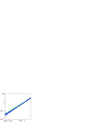
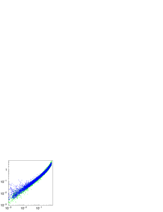
Figure 7: Ratio of branching ratios of neutralino LSP decays. To the left: Br($\mu qq^{\prime}$)/Br($\tau qq^{\prime}$) as a function of $\tan^{2}(\theta_{atm})$. To the right: Br($eqq^{\prime}$)/Br($\tau qq^{\prime}$) as a function of $U_{e3}^{2}$. Whether bilinear R-parity breaking SUSY is responsible for atmospheric neutrino oscillations can be checked by such a measurement. Note that the spread of the points is entirely due to the unknown MSSM parameters. Even a moderately accurate input of MSSM parameters will lead to much sharper predictions for these decays.

One example is shown in Fig. 7, where ratio of branching ratios of neutralino LSP decays are plotted. Note that Br($\mu qq^{\prime}$)/Br($\tau qq^{\prime}$) is directly proportional to $\tan^{2}(\theta_{atm})$, i.e. should be near $\sim 1$ according to current neutrino data. The spread in the points is due to the unknown MSSM parameters. Of course, once SUSY is discovered these unknowns will be measured allowing for much sharper tests of the model than indicated in Fig. 7.

Figure 8: Ratio of branching ratios of scalar tau LSP decays. To the left: Br(${\tilde{\tau}}_{1}\to\sum\nu e$) /Br(${\tilde{\tau}}_{1}\to\sum\nu\mu$) as a function of $(\epsilon_{1}/\epsilon_{2})^{2}$. To the right: as a function of $\tan^{2}(\theta_{\odot})$. Whether bilinear R-parity breaking SUSY is responsible for solar neutrino oscillations can be checked by such a measurement if scalar taus are the LSP.

A second example is shown in Fig. 8, where we show Br(${\tilde{\tau}}_{1}\to\sum\nu e$)/ Br(${\tilde{\tau}}_{1}\to\sum\nu\mu$) as a function of $(\epsilon_{1}/\epsilon_{2})^{2}$ (left) and as a function of $\tan^{2}(\theta_{\odot})$ (right). Obviously this ratio is strongly correlated with the solar angle and thus, if scalar taus turn out to be the LSP, such a measurement would provide an excellent check of the bilinear model as the origin of the solar neutrino mass scale.

With the LSP unstable, in principle any sparticle can be the LSP. In Hirsch:2003fe the remaining candidates have been discussed: Charginos, scalar quarks, gluinos and scalar neutrinos. The main conclusion of Hirsch:2003fe is that whichever SUSY particle is the LSP, measurements of branching ratios at future accelerators will provide a definite test of bilinear R-parity breaking as the model of neutrino mass. We just mention that chargino LSPs would be more sensitive to atmospheric neutrino physics (as are neutralinos) while the other LSP candidates mentioned above show more dependence on the solar neutrino angle.

6 Discussion and conclusions

We have presented a brief review of the idea that supersymmetry with explicit bilinear breaking of R-parity is the origin of neutrino masses and lepton mixing. The bilinear R-parity breaking (BRpV) model is the simplest extension of the minimal supersymmetric standard model (MSSM) which includes lepton number violation. We have seen how it leads to a successful phenomenological model for neutrino oscillations, in accordance to present neutrino data. The pattern of neutrino masses is hierarchical, with the atmospheric mass scale arising at the tree level whereas the solar scale is induced from calculable loop corrections. We saw how, in contrast to seesaw models, the BRpV model can be probed at future collider experiments, like the LHC or the NLC. Indeed we have discussed how, irrespective of the supersymmetric particle which is the lightest, its decay pattern will be directly related with the lepton mixing angles determined in low energy neutrino experiments.

References

• [1] Super-Kamiokande, Y. Fukuda et al., Phys. Rev. Lett. 81, 1562 (1998), [hep-ex/9807003].
• [2] SNO, Q. R. Ahmad et al., Phys. Rev. Lett. 89, 011301 (2002), [nucl-ex/0204008].
• [3] KamLAND, K. Eguchi et al., Phys. Rev. Lett. 90, 021802 (2003), [hep-ex/0212021].
• [4] M. Maltoni, T. Schwetz, M. A. Tortola and J. W. F. Valle, Prepared for this volume. Based on previous paper published in Phys. Rev. D68, 113010 (2003), [hep-ph/0309130], which also contains a more extensive list of references.
• [5] S. Pakvasa and J. W. F. Valle, hep-ph/0301061, Proceedings of the Indian National Academy of Sciences on Neutrinos, Part A: Vol. 70A, No.1, p.189 - 222 (2004), Eds. D. Indumathi, M.V.N. Murthy and G. Rajasekaran.
• [6] V. Barger, D. Marfatia and K. Whisnant, hep-ph/0308123.
• [7] M. C. Gonzalez-Garcia and Y. Nir, hep-ph/020205.
• [8] G. L. Fogli, et al., Talk at 10th International Workshop on Neutrino Telescopes, Venice, Italy, 11-14 Mar 2003, Neutrino telescopes, p. 151-179
• [9] H. P. Nilles, Phys. Rept. 110, 1 (1984).
• [10] H. E. Haber and G. L. Kane, Phys. Rept. 117, 75 (1985).
• [11] E. Witten, hep-ph/0207124.
• [12] M. Gell-Mann, P. Ramond and R. Slansky, (1979), Print-80-0576 (CERN).
• [13] T. Yanagida, (KEK lectures, 1979), ed. Sawada and Sugamoto (KEK, 1979).
• [14] J. Schechter and J. W. F. Valle, Phys. Rev. D22, 2227 (1980); Phys. Rev. D25, 774 (1982).
• [15] R. N. Mohapatra and G. Senjanovic, Phys. Rev. D23, 165 (1981).
• [16] C. S. Aulakh and R. N. Mohapatra, Phys. Lett. B119, 13 (1982).
• [17] G. G. Ross and J. W. F. Valle, Phys. Lett. B151, 375 (1985).
• [18] J. R. Ellis and et al., Phys. Lett. B150, 142 (1985).
• [19] A. Abada, S. Davidson and M. Losada, Phys. Rev. D65, 075010 (2002), [hep-ph/0111332].
• [20] Y. Grossman and H. E. Haber, hep-ph/9906310.
• [21] V. Bednyakov, A. Faessler and S. Kovalenko, Phys. Lett. B442, 203 (1998), [hep-ph/9808224].
• [22] A. S. Joshipura, R. D. Vaidya and S. K. Vempati, Nucl. Phys. B 639, 290 (2002) [arXiv:hep-ph/0203182];
C. H. Chang and T. F. Feng, Eur. Phys. J. C 12, 137 (2000) [arXiv:hep-ph/9901260].
• [23] M. A. Diaz, J. C. Romao and J. W. F. Valle, Nucl. Phys. B524, 23 (1998), [hep-ph/9706315].
• [24] M. A. Diaz et al., Phys. Rev. D68, 013009 (2003), [hep-ph/0302021].
• [25] E. J. Chun, D.-W. Jung and J. D. Park, Phys. Lett. B557, 233 (2003), [hep-ph/0211310].
• [26] M. Hirsch et al., Phys. Rev. D62, 113008 (2000), [hep-ph/0004115], Err-ibid.D65 119901 (2002).
• [27] J. C. Romao et al., Phys. Rev. D61, 071703 (2000), [hep-ph/9907499].
• [28] F. de Campos et al., Nucl. Phys. B451, 3 (1995), [hep-ph/9502237].
• [29] T. Banks, Y. Grossman, E. Nardi and Y. Nir, Phys. Rev. D52, 5319 (1995), [hep-ph/9505248].
• [30] B. de Carlos and P. L. White, Phys. Rev. D54, 3427 (1996), [hep-ph/9602381].
• [31] A. G. Akeroyd et al., Nucl. Phys. B529, 3 (1998), [hep-ph/9707395].
• [32] A. Masiero and J. W. F. Valle, Phys. Lett. B251, 273 (1990).
• [33] J. C. Romao, C. A. Santos and J. W. F. Valle, Phys. Lett. B288, 311 (1992).
• [34] J. C. Romao, A. Ioannisian and J. W. F. Valle, Phys. Rev. D55, 427 (1997), [hep-ph/9607401].
• [35] B. Mukhopadhyaya, S. Roy and F. Vissani, Phys. Lett. B443, 191 (1998), [hep-ph/9808265].
• [36] R Parity Working Group, B. Allanach et al., hep-ph/9906224.
• [37] S. Y. Choi, E. J. Chun, S. K. Kang and J. S. Lee, Phys. Rev. D60, 075002 (1999), [hep-ph/9903465].
• [38] A. Bartl et al., Nucl. Phys. B600, 39 (2001), [hep-ph/0007157].
• [39] W. Porod, M. Hirsch, J. Romao and J. W. F. Valle, Phys. Rev. D63, 115004 (2001), [hep-ph/0011248].
• [40] D. Restrepo, W. Porod and J. W. F. Valle, Phys. Rev. D64, 055011 (2001), [hep-ph/0104040].
• [41] M. Hirsch, W. Porod, J. C. Romao and J. W. F. Valle, Phys. Rev. D66, 095006 (2002), [hep-ph/0207334].
• [42] A. Bartl et al., JHEP 11, 005 (2003), [hep-ph/0306071].
• [43] M. Hirsch and W. Porod, Phys. Rev. D68, 115007 (2003), [hep-ph/0307364].
• [44] G. F. Giudice and A. Masiero, Phys. Lett. B206, 480 (1988).
• [45] H.-P. Nilles and N. Polonsky, Nucl. Phys. B484, 33 (1997), [hep-ph/9606388].
• [46] J. M. Mira, E. Nardi, D. A. Restrepo and J. W. F. Valle, Phys. Lett. B492, 81 (2000), [hep-ph/0007266].
• [47] L. E. Ibanez and G. G. Ross, Phys. Lett. B110, 215 (1982).
• [48] A. Santamaria and J. W. F. Valle, Phys. Lett. B195, 423 (1987), Phys. Rev. Lett. 60, 397 (1988), Phys. Rev. D39, 1780 (1989).
• [49] M. Hirsch and J. W. F. Valle, Nucl. Phys. B557, 60 (1999), [hep-ph/9812463].
• [50] G. Passarino and M. J. G. Veltman, Nucl. Phys. B160, 151 (1979).