New plots and parameter degeneracies in neutrino oscillations

Abstract

It is shown that eightfold degeneracy in neutrino oscillations is easily seen by plotting constant probabilities in the $(\sin^{2}2\theta_{13},1/s^{2}_{23})$ plane. Using this plot, we discuss how an additional long baseline measurement resolves degeneracies after the JPARC experiment measures the oscillation probabilities $P(\nu_{\mu}\rightarrow\nu_{e})$ and $P(\bar{\nu}_{\mu}\rightarrow\bar{\nu}_{e})$ at $|\Delta m^{2}_{31}|L/4E=\pi/2$. By measuring $P(\nu_{\mu}\rightarrow\nu_{e})$ or $P(\bar{\nu}_{\mu}\rightarrow\bar{\nu}_{e})$, the sgn($\Delta m_{31}^{2}$) ambiguity is resolved better at longer baselines and the $\delta\leftrightarrow\pi-\delta$ ambiguity is resolved better when $\left||\Delta m^{2}_{31}|L/4E-\pi/2\right|$ is larger. The $\theta_{23}$ ambiguity may be resolved as a byproduct if $\left||\Delta m^{2}_{31}|L/4E-\pi\right|$ is small and the CP phase $\delta$ turns out to satisfy $\left|\cos(\delta+|\Delta m^{2}_{31}|L/4E)\right|\sim 1$. It is pointed out that the low energy option ($E\sim$1GeV) at the off-axis NuMI experiment may be useful in resolving these ambiguities. The $\nu_{e}\rightarrow\nu_{\tau}$ channel offers a promising possibility which may potentially resolve all the ambiguities.

I Introduction

From the recent experiments on atmospheric Kajita:2001mr and solar Bahcall:2000kh , and reactor Apollonio:1999ae ; Eguchi:2002dm neutrinos, we now know approximately the values of the mixing angles and the mass squared differences of the atmospheric and solar neutrino oscillations:

$$(\sin^{2}2\theta_{12},\Delta m^{2}_{21}) \simeq (0.8,7\times 10^{-5}{\rm eV}^{2})~{}\qquad\mbox{\rm for the solar neutrino}$$

$$(\sin^{2}2\theta_{23},|\Delta m^{2}_{31}|) \simeq (1.0,2\times 10^{-3}{\rm eV}^{2})~{}\qquad\mbox{\rm for the atmospheric neutrino},$$

where we use the standard parametrization Hagiwara:pw of the MNS mixing matrix

$$U=\left(\begin{array}[]{ccc}c_{12}c_{13}&s_{12}c_{13}&s_{13}e^{-i\delta}\\ -s_{12}c_{23}-c_{12}s_{23}s_{13}e^{i\delta}&c_{12}c_{23}-s_{12}s_{23}s_{13}e^{i\delta}&s_{23}c_{13}\\ s_{12}s_{23}-c_{12}c_{23}s_{13}e^{i\delta}&-c_{12}s_{23}-s_{12}c_{23}s_{13}e^{i\delta}&c_{23}c_{13}\end{array}\right),$$ (4)

and the case of $\Delta m_{31}^{2}>0$ ($\Delta m_{31}^{2}<0$) corresponds to the normal (inverted) mass hierarchy, as is shown in Fig. 1. In the three flavor framework of neutrino oscillations, the oscillation parameters which are still unknown to date are the third mixing angle $\theta_{13}$, the sign of the mass squared difference $\Delta m^{2}_{31}$ of the atmospheric neutrino oscillation, and the CP phase $\delta$. It is expected that long baseline experiments in the future will determine these three quantities.

Since the work of Burguet-Castell:2001ez , it has been known that even if the values of the oscillation probabilities $P(\nu_{\mu}\rightarrow\nu_{e})$ and $P(\bar{\nu}_{\mu}\rightarrow\bar{\nu}_{e})$ are exactly given we cannot determine uniquely the values of the oscillation parameters due to parameter degeneracies. There are three kinds of parameter degeneracies: the intrinsic $(\theta_{13},\delta)$ degeneracy Burguet-Castell:2001ez , the degeneracy of $\Delta m^{2}_{31}\leftrightarrow-\Delta m^{2}_{31}$ Minakata:2001qm , and the degeneracy of $\theta_{23}\leftrightarrow\pi/2-\theta_{23}$ Fogli:1996pv ; Barger:2001yr . The intrinsic degeneracy is exact when $\Delta m^{2}_{21}/\Delta m^{2}_{31}$ is exactly zero. The sgn($\Delta m^{2}_{31}$) degeneracy is exact when $AL$ is exactly zero, where $A\equiv\sqrt{2}G_{F}N_{e}$ and $L$ stand for the matter effect and the baseline, respectively ($G_{F}$ is the Fermi constant and $N_{e}$ is the electron density in matter). The $\theta_{23}$ degeneracy is exact when $\cos 2\theta_{23}$ is exactly zero. Each degeneracy gives a twofold solution, so in total we have an eightfold solution if all the degeneracies are exact. In this case prediction for physics is the same for all the degenerated solutions and there is no problem. However, these degeneracies are lifted slightly in long baseline experiments , and there are in general eight different solutions Barger:2001yr . When we try to determine the oscillation parameters, ambiguities arise because the values of the oscillation parameters are slightly different for each solution. In particular, this causes a serious problem in measurement of CP violation, which is expected to be small effect in the long baseline experiments, and we could mistake a fake effect due to the ambiguities for nonvanishing CP violation if we do not treat the ambiguities carefully.

In the references Burguet-Castell:2001ez ; Minakata:2001qm ; Barger:2001yr in the past, various diagrams have been given to visualize how degeneracies are lifted in the parameter space. To see how the eightfold degeneracy is lifted, it is necessary for the plot to give eight different points for different eight solutions. An effort was made in Minakata:2002jv to visualize the eight different points by plotting the trajectories of constant probabilities in the $(\sin^{2}2\theta_{13},s^{2}_{23})$ plane. In the present paper we propose a plot in the $(\sin^{2}2\theta_{13},1/s^{2}_{23})$ plane, which offers the simplest way to visualize how the eightfold degeneracy is lifted. As a byproduct, we show how the third measurement of $\nu_{\mu}\rightarrow\nu_{e}$, $\bar{\nu}_{\mu}\rightarrow\bar{\nu}_{e}$ or $\nu_{e}\rightarrow\nu_{\tau}$ resolves the ambiguities, after the JPARC experiment Itow:2001ee measures the oscillation probabilities $P(\nu_{\mu}\rightarrow\nu_{e})$ and $P(\bar{\nu}_{\mu}\rightarrow\bar{\nu}_{e})$ at the oscillation maximum, i.e., at $|\Delta m^{2}_{31}|L/4E=\pi/2$.

In the following discussions we assume that $|\Delta m^{2}_{31}|$, $\Delta m^{2}_{21}$ and $\theta_{12}$ are sufficiently precisely known. This is justified because the correlation between these parameters and the CP phase $\delta$ is not so strong in the case of JPARC Pinney:2001xw , and we can safely ignore the uncertainty of these parameters to discuss the ambiguities in $\delta$ due to parameter degeneracies.

II Plots in the $(\sin^{2}2\theta_{13},1/s^{2}_{23})$ plane

As in Ref. Yasuda:2003qg , let us discuss the ambiguities due to degeneracies step by step in the order $(\theta_{23}-\pi/4=0,\Delta m^{2}_{21}=0,A=0)$ $\rightarrow$ $(\theta_{23}-\pi/4\neq 0,\Delta m^{2}_{21}=0,A=0)$ $\rightarrow$ $(\theta_{23}-\pi/4\neq 0,\Delta m^{2}_{21}\neq 0,A=0)$ $\rightarrow$ $(\theta_{23}-\pi/4\neq 0,\Delta m^{2}_{21}\neq 0,A\neq 0)$.

II.1 $\cos 2\theta_{23}=0,\Delta m^{2}_{21}/\Delta m^{2}_{31}=0,AL=0$

In this case the oscillation probabilities $P(\nu_{\mu}\rightarrow\nu_{e})$ and $P(\bar{\nu}_{\mu}\rightarrow\bar{\nu}_{e})$ are equal and are given by

$$P(\nu_{\mu}\rightarrow\nu_{e})=P(\bar{\nu}_{\mu}\rightarrow\bar{\nu}_{e})=s_{23}^{2}\sin^{2}2\theta_{13}\sin^{2}\Delta,$$

where we have introduced the notation

$$\Delta\equiv\frac{|\Delta m_{31}|L}{4E}.$$

To plot the line $P(\nu_{\mu}\rightarrow\nu_{e})=P(\bar{\nu}_{\mu}\rightarrow\bar{\nu}_{e})$=const. in the ($\sin^{2}2\theta_{13}$, $1/s^{2}_{23}$) plane, let us introduce the variables

$$X \equiv \sin^{2}2\theta_{13},$$

$$Y \equiv \frac{1}{s^{2}_{23}}.$$

Then

$$P=s_{23}^{2}\sin^{2}2\theta_{13}\sin^{2}\Delta$$

give a straight line

$$Y=\frac{\sin^{2}\Delta}{P}X$$ (5)

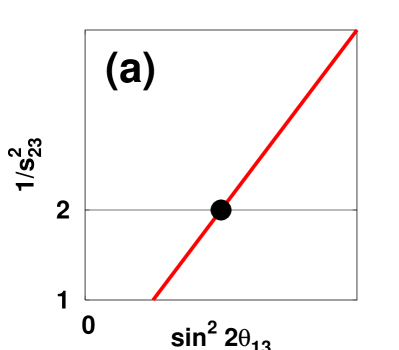
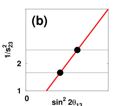
Figure 2: The solutions, which are marked by black blobs, for given $P(\nu_{\mu}\rightarrow\nu_{e})$, $P(\bar{\nu}_{\mu}\rightarrow\bar{\nu}_{e})$ and $P(\nu_{\mu}\rightarrow\nu_{\mu})$ in the case of $\Delta m^{2}_{21}/\Delta m^{2}_{31}=0,AL=0$. (a) For $\cos 2\theta_{23}=0$, the intersection of $Y\equiv 1/s^{2}_{23}=2$ and the trajectory of $P(\nu_{\mu}\rightarrow\nu_{e})=P(\nu_{\mu}\rightarrow\nu_{\mu})=$ const. is one point with eightfold degeneracy. (b) For $\cos 2\theta_{23}\neq 0$, the intersections are two solutions with fourfold degeneracy.

in the ($X$, $Y$) plane, where $P$ and $\sin^{2}\Delta$ are constant. The intersection of Eq. (5) and $Y\equiv 1/s_{23}^{2}=2$ in the ($\sin^{2}2\theta_{13}$, $1/s^{2}_{23}$) plane is a unique point, which corresponds to a solution with eightfold degeneracy. The solution is depicted in Fig. 2(a).

II.2 $\cos 2\theta_{23}\neq 0,\Delta m^{2}_{21}/\Delta m^{2}_{31}=0,AL=0$

At present the Superkamiokande atmospheric neutrino data gives the allowed region $0.90<\sin 2\theta_{23}\leq 1.0$ at 90%CL saji , and $\sin^{2}2\theta_{23}$ can be in general different from 1.0. If $\sin^{2}2\theta_{23}$, which is more accurately determined from the oscillation probability $P(\nu_{\mu}\rightarrow\nu_{\mu})$ in the future long baseline experiments, deviates from 1, then we have two solutions for $Y\equiv 1/s^{2}_{23}$:

$$Y_{+} = \frac{2}{1-\sqrt{1-\sin^{2}2\theta_{23}}}$$

$$Y_{-} = \frac{2}{1+\sqrt{1-\sin^{2}2\theta_{23}}}.$$

In this case there are two solutions, the one given by Eq. (5) and $Y=Y_{+}$ and another given by Eq. (5) and $Y=Y_{-}$. These are two solutions with fourfold degeneracy. The two solutions in the ($\sin^{2}2\theta_{13}$, $1/s^{2}_{23}$) plane are shown in Fig. 2(b). From this we see that even if we know precisely the values of $P(\nu_{\mu}\rightarrow\nu_{e})$, $P(\bar{\nu}_{\mu}\rightarrow\bar{\nu}_{e})$ and $P(\nu_{\mu}\rightarrow\nu_{\mu})$, there are two sets of solutions, and this is the ambiguity due to the $\theta_{23}\leftrightarrow\pi-\theta_{23}$ degeneracy.

II.3 $\cos 2\theta_{23}\neq 0,\Delta m^{2}_{21}/\Delta m^{2}_{31}\neq 0,AL=0$

If we turn on the effect of non-zero $\Delta m^{2}_{21}$ in addition to non-zero $\cos 2\theta_{23}$, then the oscillation probabilities are

$$\left\{\begin{array}[]{c}P(\nu_{\mu}\to\nu_{e})\\ P(\bar{\nu}_{\mu}\to\bar{\nu}_{e})\end{array}\right\}=x^{2}\sin^{2}\Delta+2xy\Delta\sin\Delta\cos\left(\delta\pm\Delta\right)+y^{2}\Delta^{2}\,,$$ (8)

which are correct to the second order in the small parameters $|\Delta m^{2}_{21}/\Delta m^{2}_{31}|$ and $\sin 2\theta_{13}$, where

$$x \equiv s_{23}\sin 2\theta_{13}\,,$$

$$y \equiv \left|\frac{\Delta m_{21}^{2}}{\Delta m_{31}^{2}}\right|c_{23}\sin 2\theta_{12}.$$ (9)

In this case, the trajectory of $P(\nu_{\mu}\to\nu_{e})=P$, $P(\bar{\nu}_{\mu}\to\bar{\nu}_{e})=\bar{P}$, where $P$ and $\bar{P}$ are constant, in the ($X\equiv\sin^{2}2\theta_{13}$, $Y\equiv 1/s^{2}_{23}$) plane is given by a quadratic curve:

$$16C_{0}X(Y-1)\Delta^{2}\sin^{2}\Delta$$ (10)

$$= \frac{1}{\sin^{2}\Delta}(P-\bar{P})^{2}Y^{2}+\frac{1}{\cos^{2}\Delta}\left[(P+\bar{P}-2C_{0})(Y-1)+P+\bar{P}-2X\sin^{2}\Delta\right]^{2},$$

where

$$C_{0}\equiv\left(\frac{\Delta m^{2}_{21}}{\Delta m^{2}_{31}}\right)^{2}\Delta^{2}\sin^{2}2\theta_{12}.$$

Eq. (10) becomes a hyperbola for most of the range of $\Delta$, but it becomes an ellipse for some region $\Delta\simeq\pi$.

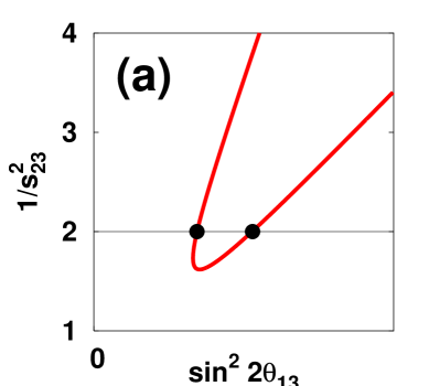
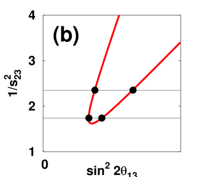
Figure 3: The solutions, which are marked by black blobs, for given $P(\nu_{\mu}\rightarrow\nu_{e})$, $P(\bar{\nu}_{\mu}\rightarrow\bar{\nu}_{e})$ and $P(\nu_{\mu}\rightarrow\nu_{\mu})$ in the case of $\Delta m^{2}_{21}/\Delta m^{2}_{31}\neq 0,AL=0$. (a) For $\cos 2\theta_{23}=0$, the intersection of $Y\equiv 1/s^{2}_{23}=2$ and the trajectory of $P(\nu_{\mu}\rightarrow\nu_{e})=$ const., $P(\nu_{\mu}\rightarrow\nu_{\mu})=$ const. are two points with fourfold degeneracy. (b) For $\cos 2\theta_{23}\neq 0$, the intersections are four solutions with twofold degeneracy.

When $\sin^{2}2\theta_{23}=1$, there are two solutions for the intersection of $Y=2$ and Eq. (10). This indicates that even if we know the precise values of $P(\nu_{\mu}\rightarrow\nu_{e})$, $P(\bar{\nu}_{\mu}\rightarrow\bar{\nu}_{e})$ and $P(\nu_{\mu}\rightarrow\nu_{\mu})$, there are two sets of solutions for $(\theta_{13},\theta_{23},\delta)$ with fourfold degeneracy when $\sin^{2}2\theta_{23}=1$, as is depicted in Fig. 3(a). This is the ambiguity due to the intrinsic $(\theta_{13},\delta)$ degeneracy. When $\sin^{2}2\theta_{23}\neq 1$, there are four sets of solutions with twofold degeneracy, as is depicted in Fig. 3(b).

II.4 $\cos 2\theta_{23}\neq 0,\Delta m^{2}_{21}/\Delta m^{2}_{31}\neq 0,AL\neq 0$

Furthermore, if we turn on the matter effect $AL$, then the oscillation probabilities are given by Cervera:2000kp ; Barger:2001yr

$$P(\nu_{\mu}\to\nu_{e}) = x^{2}f^{2}+2xyfg\cos\left(\delta+\Delta\right)+y^{2}g^{2}\,,$$

$$P(\bar{\nu}_{\mu}\to\bar{\nu}_{e}) = x^{2}\bar{f}^{2}+2xy\bar{f}g\cos\left(\delta-\Delta\right)+y^{2}g^{2}\,,$$ (11)

for the normal hierarchy, while

$$P(\nu_{\mu}\to\nu_{e}) = x^{2}\bar{f}^{2}-2xy\bar{f}g\cos\left(\delta-\Delta\right)+y^{2}g^{2}\,,$$

$$P(\bar{\nu}_{\mu}\to\bar{\nu}_{e}) = x^{2}f^{2}-2xyfg\cos\left(\delta+\Delta\right)+y^{2}g^{2}\,,$$ (12)

for the inverted hierarchy, where $x$ and $y$ are given by Eq. (9), and

$$\left\{\begin{array}[]{c}f\\ \bar{f}\end{array}\right\} \equiv \frac{\sin\left(\Delta\mp AL/2\right)}{\left(1\mp AL/2\Delta\right)}\,,$$ (15)

$$g \equiv \frac{\sin\left(AL/2\right)}{AL/2\Delta}\,.$$ (16)

Eqs. (11) and (12) are correct up to the second order in $|\Delta m^{2}_{21}/\Delta m^{2}_{31}|$ and $\sin 2\theta_{13}$, and all orders in $AL$. The trajectory of $P(\nu_{\mu}\to\nu_{e})=P$, $P(\bar{\nu}_{\mu}\to\bar{\nu}_{e})=\bar{P}$, where $P$ and $\bar{P}$ are constant, in the ($X\equiv\sin^{2}2\theta_{13}$, $Y\equiv 1/s^{2}_{23}$) plane is again a quadratic curve for either of the mass hierarchies:

$$16CX(Y-1) = \frac{1}{\cos^{2}\Delta}\left[\left(\frac{P-C}{f}+\frac{\bar{P}-C}{\bar{f}}\right)(Y-1)-(f+\bar{f})X+\frac{P}{f}+\frac{\bar{P}}{\bar{f}}\right]^{2}$$ (17)

$$+\frac{1}{\sin^{2}\Delta}\left[\left(\frac{P-C}{f}-\frac{\bar{P}-C}{\bar{f}}\right)(Y-1)-(f-\bar{f})X+\frac{P}{f}-\frac{\bar{P}}{\bar{f}}\right]^{2}$$

for the normal hierarchy, and

$$16CX(Y-1) = \frac{1}{\cos^{2}\Delta}\left[\left(\frac{P-C}{\bar{f}}+\frac{\bar{P}-C}{f}\right)(Y-1)-(f+\bar{f})X+\frac{P}{\bar{f}}+\frac{\bar{P}}{f}\right]^{2}$$ (18)

$$+\frac{1}{\sin^{2}\Delta}\left[\left(\frac{P-C}{\bar{f}}-\frac{\bar{P}-C}{f}\right)(Y-1)-(f-\bar{f})X+\frac{P}{\bar{f}}-\frac{\bar{P}}{f}\right]^{2}$$

for the inverted hierarchy, where

$$C \equiv \left(\frac{\Delta m^{2}_{21}}{\Delta m^{2}_{31}}\right)^{2}\left[\frac{\sin(AL/2)}{AL/2\Delta}\right]^{2}\sin^{2}2\theta_{12}.$$ (19)

Again these quadratic curves become hyperbolas for most of the region of $\Delta$, but they become ellipses for some $\Delta\simeq\pi$.

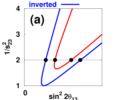
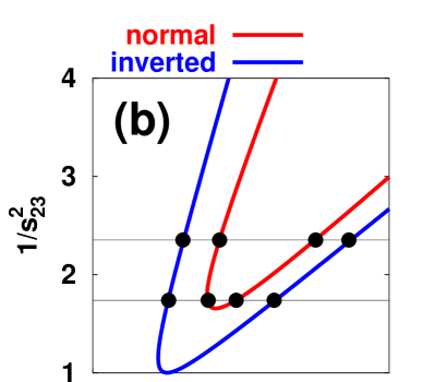
Figure 4: The solutions, which are marked by black blobs, for given $P(\nu_{\mu}\rightarrow\nu_{e})$, $P(\bar{\nu}_{\mu}\rightarrow\bar{\nu}_{e})$ and $P(\nu_{\mu}\rightarrow\nu_{\mu})$ in the case of $\Delta m^{2}_{21}/\Delta m^{2}_{31}\neq 0,AL\neq 0$. (a) For $\cos 2\theta_{23}=0$, the intersection of $Y\equiv 1/s^{2}_{23}=2$ and the trajectory of $P(\nu_{\mu}\rightarrow\nu_{e})=$ const., $P(\nu_{\mu}\rightarrow\nu_{\mu})=$ const. four points with twofold degeneracy. (b) For $\cos 2\theta_{23}\neq 0$, the intersections are eight solutions without degeneracy.

If $\sin^{2}2\theta_{23}=1$, then there are four solutions with twofold degeneracy, as is shown in Fig. 4(a). If we know for some reason (e.g., from reactor experiments) which solution is selected for each mass hierarchy, there are only two solutions. This is the ambiguity due to the sgn($\Delta m^{2}_{31}$) degeneracy. If $\sin^{2}2\theta_{23}\neq 1$ and if we do not know which solution is favored with respect to the intrinsic degeneracy for each hierarchy, and if we do not know sgn($\Delta m^{2}_{31}$), then there are eight solutions without any degeneracy, as is depicted in Fig. 4(b). The advantage of our plot is that all the eight solutions for $(\theta_{13},\theta_{23})$ give different points, and all the lines in the ($\sin^{2}2\theta_{13}$, $1/s^{2}_{23}$) plane are described by (at most) quadratic curves so that their behaviors are easy to see.

II.5 Oscillation maximum

Finally, let us consider the case where experiments are done at the oscillation maximum, i.e., when the neutrino energy$E$ satisfies $\Delta\equiv|\Delta m^{2}_{31}|L/4E=\pi/2$. In this case, the probabilities become

$$P(\nu_{\mu}\to\nu_{e}) = x^{2}f^{2}-2xyfg\sin\delta+y^{2}g^{2}\,,$$ (20)

$$P(\bar{\nu}_{\mu}\to\bar{\nu}_{e}) = x^{2}\bar{f}^{2}+2xy\bar{f}g\sin\delta+y^{2}g^{2}\,,$$ (21)

for the normal hierarchy, and

$$P(\nu_{\mu}\to\nu_{e}) = x^{2}\bar{f}^{2}-2xy\bar{f}g\sin\delta+y^{2}g^{2}\,,$$ (22)

$$P(\bar{\nu}_{\mu}\to\bar{\nu}_{e}) = x^{2}f^{2}+2xyfg\sin\delta+y^{2}g^{2}\,,$$ (23)

for the inverted hierarchy, where $x$ and $y$ are given by Eq. (9), and $f$, $\bar{f}$, $g$ in Eqs. (15), (16) become

$$\left\{\begin{array}[]{c}f\\ \bar{f}\end{array}\right\}=\pm\frac{\cos(AL/2)}{1\mp AL/\pi}\,,~{}~{}g \equiv \frac{\sin\left(AL/2\right)}{AL/\pi}$$ (26)

for $\Delta=\pi/2$. The trajectory of $P(\nu_{\mu}\to\nu_{e})=P$, $P(\bar{\nu}_{\mu}\to\bar{\nu}_{e})=\bar{P}$ in the ($X\equiv\sin^{2}2\theta_{13}$, $Y\equiv 1/s^{2}_{23}$) plane becomes a straight line and is given by

$$Y=\frac{f+\bar{f}}{P/f+\bar{P}/\bar{f}-C(1/f+1/\bar{f})}\left(X-\frac{C}{f\bar{f}}\right)$$ (27)

for the normal hierarchy, and

$$Y=\frac{f+\bar{f}}{P/\bar{f}+\bar{P}/f-C(1/f+1/\bar{f})}\left(X-\frac{C}{f\bar{f}}\right)$$ (28)

for the inverted hierarchy, where $C$ is given in Eq. (19). The straight lines (27) and (28) are extremely close to each other in relatively short long baseline experiments such as JPARC, where the matter effect is small. As is shown in Appendix B, (27) and (28) have the minimum values in $Y\equiv 1/s^{2}_{23}$ which is larger than the naive value 1 for either of the mass hierarchies. Since Eqs. (27) and (28) are linear in $X$, there is only one solution between them and $Y$=const. Thus the ambiguity due to the intrinsic degeneracy is solved by performing experiments at the oscillation maximum, although it is then transformed into another ambiguity due to the $\delta\leftrightarrow\pi-\delta$ degeneracy.

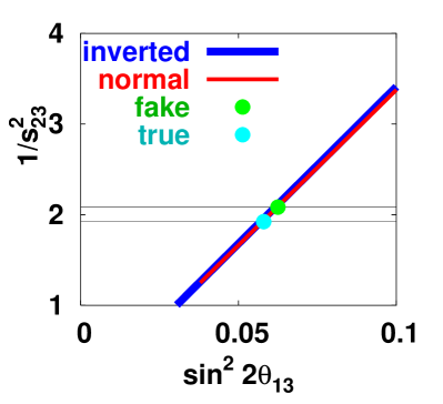
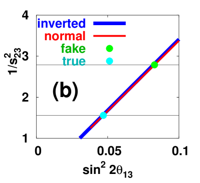
Figure 5: The $\theta_{23}$ ambiguity which could arise after the JPARC measurements of $P(\nu_{\mu}\rightarrow\nu_{e})$, $P(\bar{\nu}_{\mu}\rightarrow\bar{\nu}_{e})$ and $P(\nu_{\mu}\rightarrow\nu_{\mu})$ at the oscillation maximum. (a) If $\sin^{2}2\theta_{23}\simeq 1.0$ then the values of $\theta_{13}$ and $\theta_{23}$ are close to each other for all the solutions, and the ambiguity is not serious as far as $\theta_{13}$ and $\theta_{23}$ are concerned. (b) If $\sin^{2}2\theta_{23}<1$ then the $\theta_{23}$ ambiguity has to be resolved to determine $\theta_{13}$ and $\theta_{23}$ to good precision.

If $\sin^{2}2\theta_{23}\simeq 1$, then all the four solutions are basically close to each other in the ($\sin^{2}2\theta_{13}$, $1/s^{2}_{23}$) plane, and the ambiguity due to degeneracies are not serious as far as $\theta_{13}$ and $\theta_{23}$ are concerned (See Fig. 5(a)). On the other hand, if $\sin^{2}2\theta_{23}$ deviates fairly from 1, then the solutions are separated into two groups, those for $\theta_{23}>\pi/4$ and those for $\theta_{23}<\pi/4$ in the ($\sin^{2}2\theta_{13}$, $1/s^{2}_{23}$) plane, as is shown in Fig. 5(b). In this case resolution of the $\theta_{23}\leftrightarrow\pi/2-\theta_{23}$ ambiguity is necessary to determine $\theta_{13}$, $\theta_{23}$ and $\delta$.

II.6 Fake effects on CP violation due to degeneracies

II.6.1 $\sin^{2}2\theta_{23}\simeq 1$

If the JPARC experiment finds out from the measurement of the disappearance probability $P(\nu_{\mu}\to\nu_{\mu})=P$ that $\sin^{2}2\theta_{23}\simeq 1.0$ with a good approximation, then we would not have to worry very much about parameter degeneracy as far as $\theta_{13}$ and $\theta_{23}$ are concerned, since the values of $\theta_{13}$ and $\theta_{23}$ for all the different solutions are close to each other.

On the other hand, when it comes to the value of the CP phase phase $\delta$, we have to be careful. From Ref. Barger:2001yr the true value $\delta$ and the fake value $\delta^{\prime}$ for the CP phase satisfy the following:

$$x^{\prime}\sin\delta^{\prime} = x\sin\delta{f^{2}+\bar{f}^{2}-f\bar{f}\over f\bar{f}}-{x^{2}\over\sin\Delta}{f^{2}+\bar{f}^{2}\over f\bar{f}}{f-\bar{f}\over 2yg}\,,$$ (29)

where $x$, $y$ are given in Eq. (9), $f$, $\bar{f}$, $g$ are given in Eqs. (15) and (16), and $x^{\prime}$ is defined by

$$x^{\prime 2} = {x^{2}(f^{2}+\bar{f}^{2}-f\bar{f})-2yg(f-\bar{f})x\sin\delta\sin\Delta\over f\bar{f}}\,.$$

Eq. (29) indicates that even if $\sin\delta=0$ we have nonvanishing fake CP violating effect

$$\sin\delta^{\prime}=-x{f^{2}+\bar{f}^{2}\over f\bar{f}}{f-\bar{f}\over 2yg\sin\Delta}\sqrt{f\bar{f}\over f^{2}+\bar{f}^{2}-f\bar{f}}\,,$$ (30)

if we fail to identify the correct sign of $\Delta m^{2}_{31}$. In the case of the JPARC experiment, Eq.  (30) implies

$$\sin\delta^{\prime}\simeq-2.2\sin\theta_{13},$$

which is not negligible unless $\sin^{2}2\theta_{13}\ll 10^{-2}$. Therefore we have to know the sign of $\Delta m^{2}_{31}$ to determine the CP phase to good precision.

II.6.2 $\sin^{2}2\theta_{23}<1$

As was explained in Sect. II.5, if $\sin^{2}2\theta_{23}$ deviates fairly from 1, then we have to resolve the ambiguity due to the $\theta_{23}$ degeneracy to determine the values of $\theta_{13}$ and $\theta_{23}$. As for the value of the CP phase $\delta$, we can estimate how serious the effect of the $\theta_{23}$ ambiguity on the value of $\delta$ could be. If the true value $\delta$ is zero, then the CP phase $\delta^{\prime}$ for the fake solution can be estimated as Barger:2001yr

$$\sin 2\theta_{13}^{\prime}\sin\delta^{\prime} = \left|\frac{\Delta m^{2}_{21}}{\Delta m^{2}_{31}}\right|\frac{g(f-\bar{f})\sin 2\theta_{12}}{f\bar{f}}{\cot 2\theta_{23}\over\sin\Delta}\,,$$

where

$$\sin^{2}2\theta_{13}^{\prime} = \sin^{2}2\theta_{13}\tan^{2}\theta_{23}+\left(\frac{\Delta m^{2}_{21}}{\Delta m^{2}_{31}}\right)^{2}{g^{2}\sin^{2}2\theta_{12}\over f\bar{f}}(1-\tan^{2}\theta_{23}),$$

and $f$, $\bar{f}$, $g$ are defined in Eqs. (15) and (16). In the case of JPARC, we have

$$\left|\sin\delta^{\prime}\right|\sim\frac{1}{200}\frac{|\cot 2\theta_{23}|}{t_{23}}\frac{1}{\sin 2\theta_{13}}\lesssim\frac{1}{500}\frac{1}{\sqrt{\sin^{2}2\theta_{13}}},$$ (31)

where we have used the bound $0.90\leq\sin^{2}2\theta_{23}\leq 1.0$ from the atmospheric neutrino data in the second inequality, so that we see that the ambiguity due to the $\theta_{23}$ does not cause a serious problem on determination of $\delta$ for $\sin^{2}2\theta_{13}\gtrsim 10^{-2}$. It should be stressed, however, that the effect on CP violation due to the sgn($\Delta m^{2}_{31}$) ambiguity is also serious in this case.

III Resolution of ambiguities by the third measurement after JPARC

In this section, assuming that the JPARC experiment, which is expected to be the first superbeam experiment, measures $P(\nu_{\mu}\to\nu_{e})$ and $P(\bar{\nu}_{\mu}\to\bar{\nu}_{e})$ at the oscillation maximum $\Delta\equiv\Delta m^{2}_{31}L/4E=\pi/2$, we will discuss how the third measurement after JPARC can resolve the ambiguities by using the plot in the ($\sin^{2}2\theta_{13}$, $1/s^{2}_{23}$) plane. Resolution of the $\theta_{23}$ ambiguity has been discussed using the disappearance measurement of $P(\bar{\nu}_{e}\to\bar{\nu}_{e})$ at reactors Fogli:1996pv ; Barenboim:2002nv ; Minakata:2002jv ; Huber:2003pm ; Minakata:2003wq and the silver channel $P(\nu_{e}\to\nu_{\tau})$ at neutrino factories Donini:2002rm , but it has not been discussed much using the channel $\nu_{\mu}\to\nu_{e}$ . Here we take the following reference values for the oscillation parameters:

$$\sin^{2}2\theta_{12}=0.8,~{}~{}\sin^{2}2\theta_{13}=0.05,~{}~{}\sin^{2}2\theta_{23}=0.96,$$ (32)

$$\Delta m^{2}_{21}=7\times 10^{-5}\mbox{\rm eV}^{2},~{}~{}\Delta m^{2}_{31}=2.5\times 10^{-3}\mbox{\rm eV}^{2}>0,~{}~{}\delta=\pi/4.$$

III.1 $\nu_{\mu}\rightarrow\nu_{e}$

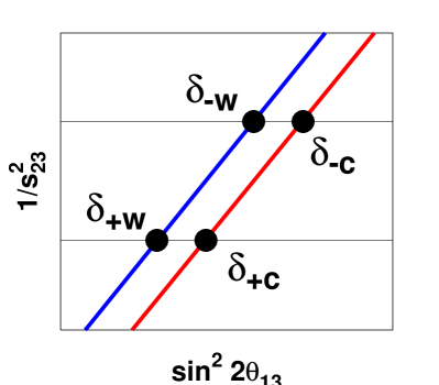
Figure 6: Four possible values for the CP phase $\delta$ at the oscillation maximum. The red (blue) line stands for the normal (inverted) hierarchy. Since we are assuming the normal hierarchy here, the red (blue) line corresponds to the correct (wrong) assumption on the mass hierarchy. $\pm$ sign stands for the choice of $s^{2}_{23}=(1\pm\sqrt{1-\sin^{2}2\theta_{23}})/2$ in the $\theta_{23}$ ambiguity, and c (w) stands for the correct (wrong) assumption on the mass hierarchy.

Let us discuss the case in which another long baseline experiment measures $P(\nu_{\mu}\to\nu_{e})$. From the measurements of $P(\nu_{\mu}\to\nu_{e})$ and $P(\bar{\nu}_{\mu}\to\bar{\nu}_{e})$ by JPARC at the oscillation maximum we can deduce the value of $\delta$, up to the eightfold ambiguity ($\delta\leftrightarrow\pi-\delta$, $\theta_{23}\leftrightarrow\pi/2-\theta_{23}$, $\Delta m^{2}_{31}\leftrightarrow-\Delta m^{2}_{31}$). As is depicted in Fig. 6, depending on whether $s^{2}_{23}-1/2$ is positive or negative, we assign the subscript $\pm$, and depending on whether our ansatz for sgn($\Delta m^{2}_{31}$) is correct or wrong, we assign the subscript c or w. Thus the eight possible values of $\delta$ are given by

$$\delta_{+\text{w}},\delta_{+\text{c}},\delta_{-\text{w}},\delta_{-\text{c}},\pi-\delta_{+\text{w}},\pi-\delta_{+\text{c}},\pi-\delta_{-\text{w}},\pi-\delta_{-\text{c}}.$$ (33)

Now suppose that the third measurement gives the value $P$ for the oscillation probability $P(\nu_{\mu}\to\nu_{e})$. Then there are in general eight lines in the ($X\equiv\sin^{2}2\theta_{13}$, $Y\equiv 1/s^{2}_{23}$) plane given by

$$f^{2}X = \left[P-C+2C\cos^{2}(\delta+\Delta)\right](Y-1)+P$$ (34)

$$-2\cos(\delta+\Delta)\sqrt{C(Y-1)}\sqrt{\left[P-C\sin^{2}(\delta+\Delta)\right](Y-1)+P}$$

for the normal hierarchy, and

$$\bar{f}^{2}X = \left[P-C+2C\cos^{2}(\delta-\Delta)\right](Y-1)+P$$ (35)

$$-2\cos(\delta-\Delta)\sqrt{C(Y-1)}\sqrt{\left[P-C\sin^{2}(\delta-\Delta)\right](Y-1)+P}$$

for the inverted hierarchy, where $C$ is defined in Eq. (19), $\Delta\equiv|\Delta m^{2}_{31}|L/4E$ is defined for the third measurement, and $\delta$ takes one of the eight values given in Eq. (33). The derivation of (34) and (35) is given in Appendix A. It turns out that the solutions (34) and (35) are hyperbola if $\cos^{2}(\delta\pm\Delta)>(C-P)/P$, where $+$ and $-$ refer to the normal and inverted hierarchy, and ellipses if $\cos^{2}(\delta\pm\Delta)<(C-P)/P$. In practice, however, the difference between hyperbola and ellipses is not so important for the present discussions, because we are only interested in the behaviors of these curves in the region $1.52<Y\equiv 1/s^{2}_{23}<2.92$ which comes from the 90%CL allowed region of the Superkamiokande atmospheric neutrino data for $\sin^{2}2\theta_{23}$.

Here let us look at three typical cases: $L$=295km, $L$=730km, $L$=3000km, each of which corresponds to JPARC, off-axis NuMI Ayres:2002nm , and a neutrino factory Geer:1997iz

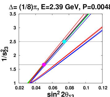
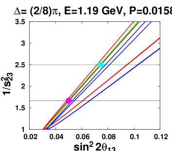
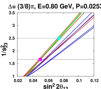
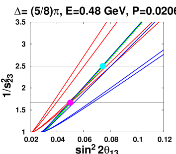
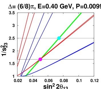
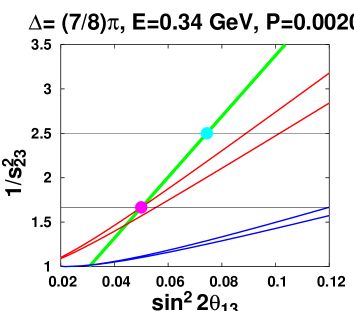
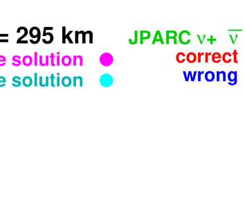
Figure 7: The trajectories of $P(\nu_{\mu}\rightarrow\nu_{e})=$ const. of the third experiment at $L$=295km with $\Delta\equiv|\Delta m^{2}_{31}|L/4E=(j/8)\pi~{}(0\leq j\leq 7,j\neq 4)$ after JPARC. The true values are those in Eq. (32). The green line is the JPARC result obtained by $P(\nu_{\mu}\rightarrow\nu_{e})$ and $P(\bar{\nu}_{\mu}\rightarrow\bar{\nu}_{e})$ at the oscillation maximum. The red (blue) lines are the trajectories of $P(\nu_{\mu}\rightarrow\nu_{e})$ given by the third experiment assuming the normal (inverted) hierarchy, where $\delta$ takes four values for each mass hierarchy.

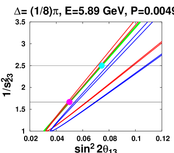
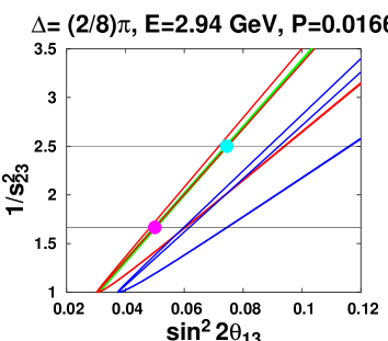
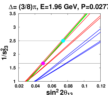
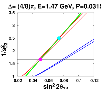
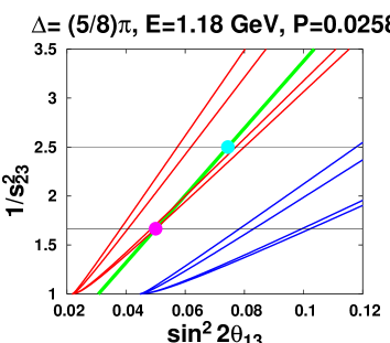
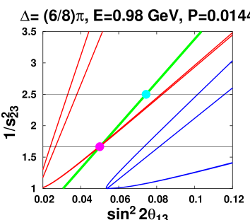
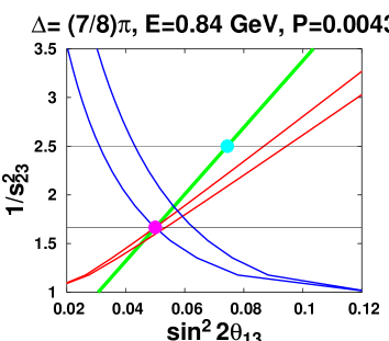
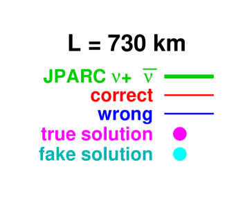
Figure 8: The trajectories of $P(\nu_{\mu}\rightarrow\nu_{e})=$ const. of the third experiment at $L$=730km with $\Delta\equiv|\Delta m^{2}_{31}|L/4E=(j/8)\pi~{}(0\leq j\leq 7)$ after JPARC. The true values are those in Eq. (32).

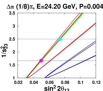
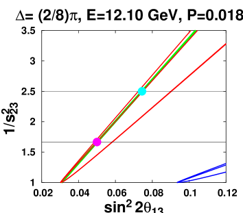
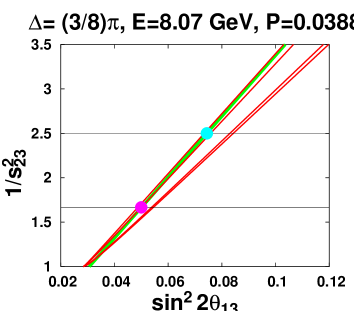
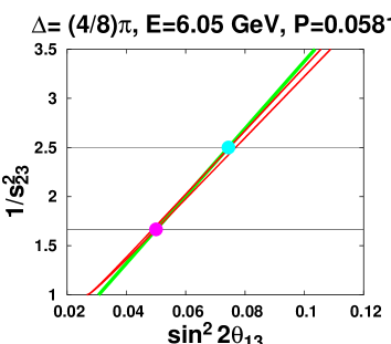
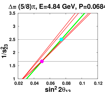
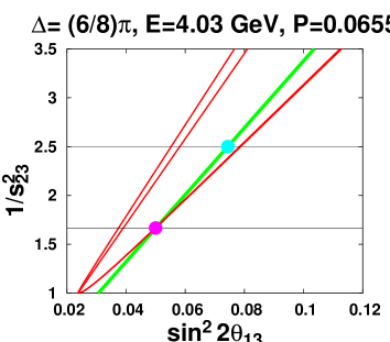
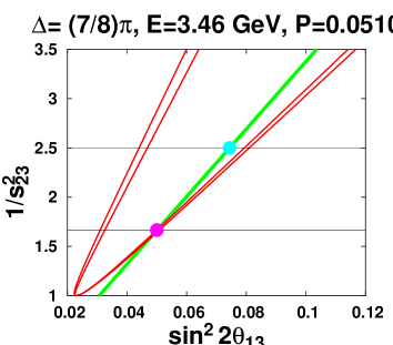
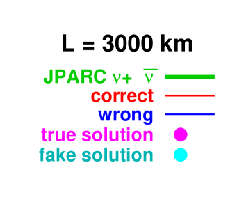
Figure 9: The trajectories of $P(\nu_{\mu}\rightarrow\nu_{e})=$ const. of the third experiment at $L$=3000km with $\Delta\equiv|\Delta m^{2}_{31}|L/4E=(j/8)\pi~{}(0\leq j\leq 7)$ after JPARC. The true values are those in Eq. (32). For $\Delta\geq(3/8)\pi$, the blue curves (with the wrong assumption for the mass hierarchy) are not in the figure because they are far to the right.

Figs. 7,8,9 show the trajectories of $P(\nu_{\mu}\to\nu_{e})$ obtained in the third measurement together with the constraint of $P(\nu_{\mu}\to\nu_{e})$, $P(\bar{\nu}_{\mu}\to\bar{\nu}_{e})$ and $P(\nu_{\mu}\to\nu_{\mu})$ by JPARC, for $L$=295km, $L$=730km, $L$=3000km, respectively, where $\Delta\equiv|\Delta m^{2}_{31}|L/4E$ takes the values $\Delta=j\pi/8$ ($j=1,\cdots,7$). The purple (light blue) blob stands for the true (fake) solution given by the JPARC results on $P(\nu_{\mu}\to\nu_{e})$, $P(\bar{\nu}_{\mu}\to\bar{\nu}_{e})$ and $P(\nu_{\mu}\to\nu_{\mu})$. For the correct (wrong) guess on the mass hierarchy, there are in general four red (blue) curves because the CP phase $\delta$, which is deduced from the JPARC results on $P(\nu_{\mu}\to\nu_{e})$, $P(\bar{\nu}_{\mu}\to\bar{\nu}_{e})$ and $P(\nu_{\mu}\to\nu_{\mu})$, is fourfold: ($\delta_{+\text{c}}$, $\delta_{-\text{c}}$, $\pi-\delta_{+\text{c}}$, $\pi-\delta_{-\text{c}}$) for the correct assumption on the hierarchy and ($\delta_{+\text{w}}$, $\delta_{-\text{w}}$, $\pi-\delta_{+\text{w}}$, $\pi-\delta_{-\text{w}}$) for the wrong assumption. In most cases the four (red or blue) curves are separated into two pairs of curves. As we will see later, the large split is due to the $\delta\leftrightarrow\pi-\delta$ ambiguity, while the small split is due to the $\theta_{23}\leftrightarrow\pi/2-\theta_{23}$ ambiguity. The reason that the latter splitting is small is because the difference of the values in the CP phases is small, as is seen from Eq. (31). In some of the figures in Figs. 7,8,9 the number of the red or blue curves is less than four because not all values of $\delta$ give consistent solutions for a set of the oscillation parameters.

Let us discuss each ambiguity one by one.

III.1.1 $\delta\leftrightarrow\pi-\delta$ ambiguity

As was mentioned above, the large splitting of four (red or blue) lines into two pair of lines is due to the $\delta\leftrightarrow\pi-\delta$ ambiguity. From Eqs. (34) and (35) we see that the only difference of the solutions with $\delta$ and with $\pi-\delta$ appears in $\cos(\delta\pm\Delta)$ or $\sin(\delta\pm\Delta)$. If $\Delta=\pi/2$ (i.e., the oscillation maximum), we have $\cos(\delta+\Delta)=-\sin\delta$, $\cos(\pi-\delta+\Delta)=-\sin\delta$, so that the values of $X$ with $\delta$ and with $\pi-\delta$ are the same, i.e., at oscillation maximum there is exact $\delta\leftrightarrow\pi-\delta$ degeneracy. On the other hand, if $\Delta\neq\pi/2$, we have $\cos(\delta+\Delta)\neq\cos(\pi-\delta+\Delta)$, and the values of $X$ with $\delta$ and with $\pi-\delta$ are different. Thus, to resolve the $\delta\leftrightarrow\pi-\delta$ ambiguity it is advantageous to perform an experiment at $\Delta$ which is farther away from $\pi/2$. Deviation of $\Delta$ from $\pi/2$ implies either high energy or low energy. In general the number of events increases for high energy because both the cross section and the neutrino flux increase, so the high energy option is preferred to resolve the $\delta\leftrightarrow\pi-\delta$ ambiguity .

III.1.2 $\Delta m^{2}_{31}\leftrightarrow-\Delta m^{2}_{31}$ ambiguity

As one can easily imagine, the sgn($\Delta m^{2}_{31}$) ambiguity is resolved better with longer baselines, since the dimensionless quantity $AL\equiv\sqrt{2}G_{F}N_{e}L\sim(L/1900$km)($\rho/2.7$g$\cdot$cm${}^{-3})$ becomes of order one for $L\gtrsim$1000km. On the other hand, from Figs. 8 and 9, we observe that the split of the curves with the different mass hierarchies (the red vs blue curves) is larger for lower energy. Naively this appears to be counterintuitive, because at low energy the matter effect is expected to be less important ($|\Delta m^{2}_{31}|L/4E\gg AL$). However, this is not the case because we are dealing with the value of $\sin^{2}2\theta_{13}$ which is obtained for a given value of $P(\nu_{\mu}\to\nu_{e})$. To see this, let us consider for simplicity the the value of $X\equiv\sin^{2}2\theta_{13}$ at $Y\equiv 1/s^{2}_{23}=1$, i.e., the X-intercept of the quadratic curves at $Y=1$. $(\sin^{2}2\theta_{13})_{n}$ ($(\sin^{2}2\theta_{13})_{i}$) at $Y=1$ for the normal (inverted) hierarchy is given by $x^{2}$ by putting $y=0$ in Eq. (11) (Eq. (12)):

$$(\sin^{2}2\theta_{13})_{n} = \frac{P}{f^{2}}$$

$$\qquad\qquad\qquad\mbox{\rm for}~{}s^{2}_{23}=1$$

$$(\sin^{2}2\theta_{13})_{i} = \frac{P}{\bar{f}^{2}}.$$

The ratio of these two quantities is given for small $AL$ by

$$\frac{(\sin^{2}2\theta_{13})_{n}}{(\sin^{2}2\theta_{13})_{i}} = \frac{f^{2}}{\bar{f}^{2}}=\frac{\sin^{2}\left(\Delta-AL/2\right)}{\sin^{2}\left(\Delta+AL/2\right)}\left(\frac{1+AL/2\Delta}{1-AL/2\Delta}\right)^{2}$$

$$\simeq 1+2AL\left(\frac{1}{\Delta}-\frac{1}{\tan\Delta}\right),$$

so that the larger $\Delta$ is (the smaller the neutrino energy is), the larger this ratio becomes, as long as $\Delta$ does not exceed $\pi$. This phenomenon suggests that it is potentially possible to enhance the matter effect by performing an experiment at low energy ($\Delta>\pi/2$) even with $L$=730km, and it may enable us to determine the sign of $\Delta m^{2}_{31}$ at the off-axis NuMI experiment. While the neutrino flux decreases for low energy at the off-axis NuMI experiment, the cross section at $E\sim$1GeV is not particularly small compared to higher energy, so the low energy possibility at the off-axis NuMI experiment deserves serious study.

III.1.3 $\theta_{23}\leftrightarrow\pi/2-\theta_{23}$ ambiguity

Figs. 7,8,9, which are plotted for $\delta=\pi/4$, suggest that there is a tendency in which the slope of the red curve which goes through the true point (the purple blob) is almost the same for high energy as that of the straight green line obtained by JPARC, while for the low energy the slope of the red curve is smaller than that of the JPARC green line. Here we will discuss the $X$-intercept at $Y=1$ instead of calculating the slope itself, because it is easier to consider the $X$-intercept and because the difference in the $X$-intercepts inevitably implies the different slopes for the two lines, as almost all the curves are approximately straight lines. In the case of JPARC, the matter effect is small ($AL\simeq 0.08$) so that we can put $f\simeq\bar{f}\simeq 1$. From Eq. (27) we have the $X$-intercept at $Y=1$

$$X_{\text{JPARC}}=\frac{P/f+\bar{P}/\bar{f}}{f+\bar{f}}\simeq\frac{P+\bar{P}}{2}\simeq x^{2},$$ (36)

where the term $g^{2}y^{2}$ has been ignored for simplicity. On the other hand, for the third measurement, from Eq. (34) we have

$$X_{\text{3rd}}=\frac{P}{f^{2}}\simeq x^{2}+2\frac{g}{f}xy\cos(\delta+\Delta),$$ (37)

where the term $g^{2}y^{2}$ has been ignored again for simplicity. Eq. (37) indicates that it is the second term in Eq. (37) that deviates the intercept $X_{\text{3rd}}$ of the red line from the intercept $X_{\text{JPARC}}$ of the JPARC green line. In order for the difference between $X_{\text{JPARC}}$ and $X_{\text{3rd}}$ to be large, $f$ has to be small and $|\cos(\delta+\Delta)|$ has to be large. When $AL$ is small, in order for $f$ to be small, $\left||\Delta m^{2}_{31}|L/4E-\pi\right|$ has to be small. This is one of the conditions to resolve the $\theta_{23}$ ambiguity. Here we are using the reference value $\delta=\pi/4$, so the deviation becomes maximal if $|\delta+\Delta|=|\pi/4+\Delta|\simeq\pi$. In real experiments, however, nobody knows the value of the true $\delta$ in advance, so it is difficult to design a long baseline experiment to resolve the $\theta_{23}\leftrightarrow\pi/2-\theta_{23}$ ambiguity. If $\delta$ turns out to satisfy $|\cos(\delta+\Delta)|\sim 1$ in the result of the third experiment, then we may be able to resolve the $\theta_{23}$ ambiguity as a byproduct.

III.2 $\bar{\nu}_{\mu}\rightarrow\bar{\nu}_{e}$

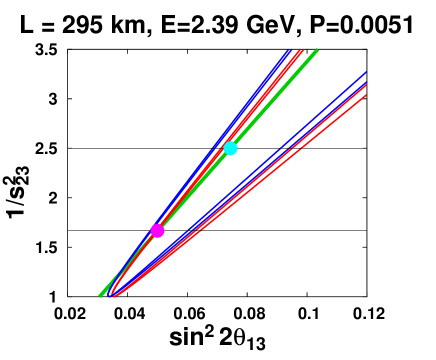
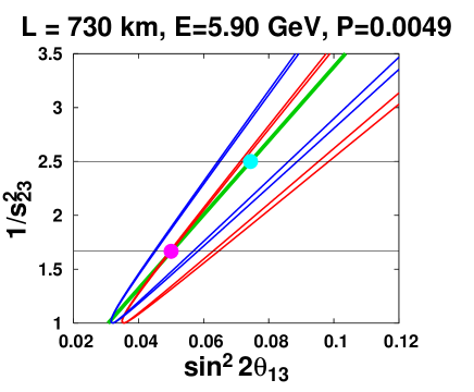
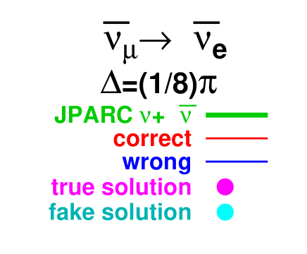
Figure 10: The trajectories of $P(\bar{\nu}_{\mu}\rightarrow\bar{\nu}_{e})=$ const. of the third experiment with $\Delta\equiv|\Delta m^{2}_{31}|L/4E=\pi/8$ after JPARC. The behaviors are almost similar to those for $P(\nu_{\mu}\rightarrow\nu_{e})=$ const. The true values are those in Eq. (32).

It turns out that the situation does not change very much even if we use the $\bar{\nu}_{\mu}\rightarrow\bar{\nu}_{e}$ channel in the third experiment. Typical curves are given for $\bar{\nu}_{\mu}\rightarrow\bar{\nu}_{e}$ in Fig. 10, which are similar to those in Fig. 7,8,9. Thus the conclusions drawn on resolution of the ambiguities hold qualitatively in the case of $\bar{\nu}_{\mu}\rightarrow\bar{\nu}_{e}$ channel.

III.3 $\nu_{e}\rightarrow\nu_{\tau}$

The experiment with the channel $\nu_{e}\rightarrow\nu_{\tau}$ requires intense $\nu_{e}$ beams and it is expected that such measurements can be done at neutrino factories or at beta beam experiments Zucchelli:sa . The oscillation probability $P(\nu_{e}\rightarrow\nu_{\tau})$ is given by

$$P(\nu_{e}\rightarrow\nu_{\tau})={\tilde{x}}^{2}f^{2}+2fg{\tilde{x}}{\tilde{y}}\cos(\delta+\Delta)+{\tilde{y}}^{2}g^{2},$$

where

$${\tilde{x}} \equiv c_{23}\sin 2\theta_{23}$$

$${\tilde{y}} \equiv \left|\frac{\Delta m^{2}_{21}}{\Delta m^{2}_{31}}\right|s_{23}\sin 2\theta_{12},$$

and $f$, $g$ are given in Eqs. (15) and (16). The solution for $P(\nu_{e}\rightarrow\nu_{\tau})=Q$, where $Q$ is constant, is given by

$$X = \frac{Q}{f^{2}}\left\{\left[1+\frac{2\cos^{2}(\delta+\Delta)}{1-C/Q}\right]\frac{1-C/Q}{Y-1}+1\right.$$ (38)

$$-\left.\frac{2\cos(\delta+\Delta)}{\sqrt{1-C/Q}}\sqrt{\left[1+\frac{\cos^{2}(\delta+\Delta)}{1-C/Q}\right]\frac{1-C/Q}{Y-1}+1}\right\},$$

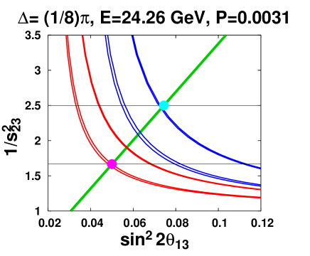
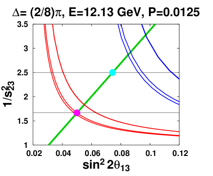
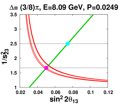
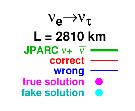
Figure 11: The trajectories of $P(\nu_{e}\rightarrow\nu_{\tau})=$ const. of the third experiment at $L$=2810km with $\Delta\equiv|\Delta m^{2}_{31}|L/4E=(j/8)\pi~{}(j=1,2,3)$ after JPARC. The true values are those in Eq. (32). The curves intersect with the JPARC line perpendicularly, so this channel is advantageous to resolve the ambiguities from experimental point of view.

where $X\equiv\sin^{2}2\theta_{13}$, $Y\equiv 1/s^{2}_{23}$ as before and $C$ is given in Eq. (19). Eqs. (38) is plotted in Fig. 11 in the case of $L$=2810km. From Fig. 11 we see that the curve $P(\nu_{e}\rightarrow\nu_{\tau})=Q$ intersects with the JPARC green line almost perpendicularly, and it is experimentally advantageous. Namely, in real experiments all the measured quantities have errors and the curves become thick. In this case the allowed region is small area around the true solution in the $(\sin^{2}2\theta_{13},1/s^{2}_{23})$ plane and one expects that the fake solution with respect to the $\theta_{23}$ ambiguity can be excluded. This is in contrast to the case of the $\nu_{\mu}\rightarrow\nu_{e}$ and $\bar{\nu}_{\mu}\rightarrow\bar{\nu}_{e}$ channels, in which the slope of the red curves is almost the same as that of the JPARC green line and the allowed region can easily contain both the true and fake solutions, so that it becomes difficult to distinguish the true point from the fake one.

As in the case of the $\nu_{\mu}\rightarrow\nu_{e}$ channel, the $\delta\leftrightarrow\pi-\delta$ ambiguity is expected to be resolved more likely for the larger value of $|\Delta-\pi/2|$, and the sgn($\Delta m^{2}_{31}$) ambiguity is resolved easily for larger baseline $L$ (e.g., $L\sim$3000km).

Thus the measurement of the $\nu_{e}\rightarrow\nu_{\tau}$ channel is a promising possibility as a potentially powerful candidate to resolve parameter degeneracies in the future.

IV Discussion and Conclusion

In this paper we have shown that the eightfold parameter degeneracy in neutrino oscillations can be easily seen by plotting the trajectory of constant probabilities in the ($\sin^{2}2\theta_{13}$, $1/s^{2}_{23}$) plane. Using this plot, we have seen that the third measurement after the JPARC results on $P(\nu_{\mu}\rightarrow\nu_{e})$ and $P(\bar{\nu}_{\mu}\rightarrow\bar{\nu}_{e})$ may resolve the sgn($\Delta m_{31}^{2}$) ambiguity at $L\gtrsim$1000km, the $\delta\leftrightarrow\pi-\delta$ ambiguity off the oscillation maximum ($\left|\Delta-\pi/2\right|\sim{\cal O}(1)$), and the $\theta_{23}$ ambiguity if $\left||\Delta m^{2}_{31}|L/4E-\pi\right|$ is small and $\delta$ turns out to satisfy $\left|\cos(\delta+\Delta)\right|\sim 1$. In general all these constraints on $\Delta\equiv|\Delta m^{2}_{31}|L/4E$ may be satisfied by taking $\Delta=\pi$. The condition $\Delta=\pi$, however, actually corresponds to the oscillation minimum, and the number of events is expected to be small for a number of reasons: (1) The probability itself is small at the oscillation minimum; (2) $\Delta=\pi$ implies low energy and the neutrino flux decreases at low energy; (3) The cross section is in general smaller at low energy than that at high energy. Therefore, to gain statistics, it is presumably wise to perform an experiment at $\pi/2<\Delta<\pi$ after JPARC. The off-axis NuMI experiment with $\pi/2<\Delta<\pi$ ($E\sim$1GeV) may have advantage to resolve these ambiguities.

As is seen in Figs. 8 and 9, the experiments at the oscillation maximum does not appear to be useful after JPARC except for the sgn($\Delta m_{31}^{2}$) ambiguity. In order to achieve other goals such as resolution of the $\delta\leftrightarrow\pi-\delta$ ambiguity and the $\theta_{23}$ ambiguity, it is wise to stay away from $\Delta=\pi/2$ in experiments after JPARC.

Although only the oscillation probabilities were discussed without taking the statistical and systematic errors into account in this paper, we hope that the present work gives some insight on how the ambiguities may be resolved in the future long baseline experiments.

Appendix A Expression for $P(\nu_{\mu}\rightarrow\nu_{e})=P$

First of all, let us derive Eqs. (34) and (35). For the normal hierarchy, the probability $P(\nu_{\mu}\to\nu_{e})=P$ is given by

$$P = P(\nu_{\mu}\to\nu_{e})=x^{2}f^{2}+2xyfg\cos\left(\delta+\Delta\right)+y^{2}g^{2}$$ (39)

$$= f^{2}\frac{X}{Y}+2f\sqrt{\frac{X}{Y}}\sqrt{C\left(1-\frac{1}{Y}\right)}\cos\left(\delta+\Delta\right)+C\left(1-\frac{1}{Y}\right),$$

where $X\equiv\sin^{2}2\theta_{13}$, $Y\equiv 1/s^{2}_{23}$ as in the text, $f$ is defined in Eq. (15), and $C$ is given in Eq. (19). Eq. (39) is rewritten as

$$(P-C)(Y-1)+P-f^{2}X=2\sqrt{f^{2}X}\sqrt{C(Y-1)}\cos\left(\delta+\Delta\right).$$ (40)

Taking the square of the both hand sides of Eq. (40), we get

$$(f^{2}X)^{2}-2f^{2}X\left\{\left[P-C+2C\cos^{2}\left(\delta+\Delta\right)\right](Y-1)+P\right\}+\left[(P-C)(Y-1)+P\right]^{2}=0.$$

Solving this quadratic equation, we obtain

$$f^{2}X = \left[P-C+2C\cos^{2}\left(\delta+\Delta\right)\right](Y-1)+P$$ (41)

$$\pm\sqrt{\left\{\left[P-C+2C\cos^{2}\left(\delta+\Delta\right)\right](Y-1)+P\right\}-\left[(P-C)(Y-1)+P\right]^{2}}$$

$$= \left[P-C+2C\cos^{2}\left(\delta+\Delta\right)\right](Y-1)+P$$

$$\pm 2\cos\left(\delta+\Delta\right)\sqrt{C(Y-1)}\sqrt{\left[P-C+C\cos^{2}\left(\delta+\Delta\right)\right](Y-1)+P}.$$

If $\cos\left(\delta+\Delta\right)>0$ then from Eq. (40) we see that $(P+C)(Y-1)+P-f^{2}X$ has to be positive. On the other hand, Eq. (41) gives

$$(P+C)(Y-1)+P-f^{2}X$$ (42)

$$= \mp 2\cos\left(\delta+\Delta\right)\sqrt{C(Y-1)}$$

$$\times\left\{\sqrt{\left[P-C+C\cos^{2}\left(\delta+\Delta\right)\right](Y-1)+P}-\cos\left(\delta+\Delta\right)\sqrt{C(Y-1)}\right\}.$$

From Eq. (42) we conclude that we have to take the minus sign in Eq. (41) for the right hand side of Eq. (42) to be positive. Hence from $P(\nu_{\mu}\to\nu_{e})=P$ we get

$$f^{2}X = \left[P-C+2C\cos^{2}(\delta+\Delta)\right](Y-1)+P$$ (43)

$$-2\cos(\delta+\Delta)\sqrt{C(Y-1)}\sqrt{\left[P-C\sin^{2}(\delta+\Delta)\right](Y-1)+P},$$

and from $P(\bar{\nu}_{e}\to\bar{\nu}_{\mu})=\bar{P}$ we have

$$\bar{f}^{2}X = \left[\bar{P}-C+2C\cos^{2}(\delta-\Delta)\right](Y-1)+\bar{P}$$ (44)

$$-2\cos(\delta-\Delta)\sqrt{C(Y-1)}\sqrt{\left[\bar{P}-C\sin^{2}(\delta-\Delta)\right](Y-1)+\bar{P}}.$$

When $P-C\sin^{2}(\delta+\Delta)>0$, Eq. (43) is a hyperbola, and the physical region for $Y-1$ is $Y-1\geq 0$. On the other hand, when $P-C\sin^{2}(\delta+\Delta)<0$, Eq. (43) becomes an ellipse and the physical region for $Y-1$ is $0\leq Y-1\leq P/[C\sin^{2}(\delta+\Delta)-P]$.

Similarly, we obtain for the inverted hierarchy:

$$\bar{f}^{2}X = \left[P-C+2C\cos^{2}(\delta-\Delta)\right](Y-1)+P$$ (45)

$$+2\cos(\delta-\Delta)\sqrt{C(Y-1)}\sqrt{\left[P-C\sin^{2}(\delta-\Delta)\right](Y-1)+P},$$

$$f^{2}X = \left[\bar{P}-C+2C\cos^{2}(\delta+\Delta)\right](Y-1)+\bar{P}$$ (46)

$$+2\cos(\delta+\Delta)\sqrt{C(Y-1)}\sqrt{\left[\bar{P}-C\sin^{2}(\delta+\Delta)\right](Y-1)+\bar{P}}.$$

Appendix B Trajectories at the oscillation maximum

Throughout this appendix we will assume $\Delta=\pi/2$ and we will assume $\Delta m^{2}_{31}>0$ for most part of this appendix. From Eq. (43), the condition $P(\nu_{\mu}\to\nu_{e})=P$ for the neutrino mode alone gives

$$f^{2}X = \left[P-C+2C\sin^{2}\delta\right](Y-1)+P$$ (47)

$$+2\sin\delta\sqrt{C(Y-1)}\sqrt{\left[P-C\cos^{2}\delta\right](Y-1)+P},$$

while the condition $P(\bar{\nu}_{\mu}\to\bar{\nu}_{e})=\bar{P}$ for the anti-neutrino mode alone gives

$$\bar{f}^{2}X = \left[\bar{P}-C+2C\sin^{2}\delta\right](Y-1)+\bar{P}$$ (48)

$$-2\sin\delta\sqrt{C(Y-1)}\sqrt{\left[\bar{P}-C\cos^{2}\delta\right](Y-1)+\bar{P}}.$$

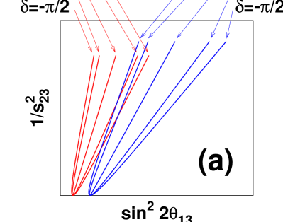
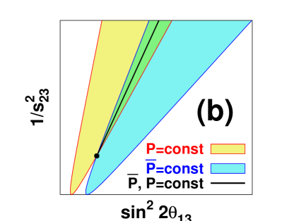
Figure 12: The region of constant probabilities at the oscillation maximum. (a) Each red (blue) line stands for $P(\nu_{\mu}\rightarrow\nu_{e})=$ const. ($P(\bar{\nu}_{\mu}\rightarrow\bar{\nu}_{e})=$ const.) for a specific value of $\delta$. The red line on the right (left) edge corresponds to $\delta=+\pi/2$ ($\delta=-\pi/2$), while the blue line on the edge right (left) corresponds to $\delta=-\pi/2$ ($\delta=+\pi/2$). (b) When $\delta$ varies from $0$ to $2\pi$, the line $P(\nu_{\mu}\rightarrow\nu_{e})=$ const. sweeps out the yellow region, whereas the line $\bar{\nu}_{\mu}\rightarrow\bar{\nu}_{e})=$ const. sweeps out the light blue region. The black straight line, which is given by $P(\nu_{\mu}\rightarrow\nu_{e})=$ const. and $P(\bar{\nu}_{\mu}\rightarrow\bar{\nu}_{e})=$ const., lies in the overlapping green region.

When $\delta$ ranges from $-\pi/2$ to $\pi/2$, Eq. (47) sweeps out the inside of a hyperbola, as is depicted by the red curves in Fig. 12(a), while (48) sweeps out the inside of another hyperbola for the anti-neutrino mode (cf. the blue curves in Fig. 12(a)). Notice that the left (right) edge of the hyperbola (47) for the neutrino mode corresponds to $\delta=-\pi/2$ ($\delta=+\pi/2$) whereas the left (right) edge of the other hyperbola (48) for the anti-neutrino mode corresponds to $\delta=+\pi/2$ ($\delta=-\pi/2$). Since the straight line (27) is the intersection of the two regions (the yellow and light blue regions in Fig. 12(b)), the lowest point in the straight line is obtained by putting $\delta=+\pi/2$ ($\delta=-\pi/2$) if $P/f^{2}<\bar{P}/\bar{f}^{2}$ (if $P/f^{2}>\bar{P}/\bar{f}^{2}$), respectively, depending on whether the region for the anti-neutrino mode is to the right of that for the neutrino mode. Therefore, if $P/f^{2}<\bar{P}/\bar{f}^{2}$, then putting $\delta=+\pi/2$ in Eqs. (20) and (21) and assuming $xf>yg$, which should hold if $\sin^{2}2\theta_{13}$ is not so small, we get

$$\sqrt{P}=xf-yg=f\sqrt{\frac{X}{Y}}-\sqrt{C\left(1-\frac{1}{Y}\right)}$$

$$\sqrt{\bar{P}}=x\bar{f}+yg=\bar{f}\sqrt{\frac{X}{Y}}+\sqrt{C\left(1-\frac{1}{Y}\right)}$$

which lead to the minimum value of $Y$

$$Y^{\text{(n)}}_{\text{min}}=\left[1-\frac{(f\sqrt{\bar{P}}-\bar{f}\sqrt{P})^{2}}{C(f+\bar{f})^{2}}\right]^{-1}$$

for the normal hierarchy. On the other hand, for the inverted hierarchy, the corresponding values of $\delta$ for the edges for the two modes are the same as those for the normal hierarchy ($\delta=\pm\pi/2$). Hence, if $P/\bar{f}^{2}<\bar{P}/f^{2}$, then putting $\delta=+\pi/2$ in Eqs. (22) and (23) and assuming $x\bar{f}>yg$, we obtain

$$\sqrt{P}=x\bar{f}-yg$$

$$\sqrt{\bar{P}}=xf+yg$$

which leads to the minimum value of $Y$

$$Y^{\text{(i)}}_{\text{min}}=\left[1-\frac{(\bar{f}\sqrt{\bar{P}}-f\sqrt{P})^{2}}{C(f+\bar{f})^{2}}\right]^{-1}$$

for $\Delta m^{2}_{31}<0$.

Figure 1: Two mass patterns. (a), (b) correspond to the normal ($\Delta m^{2}_{31}>0$), inverted ($\Delta m^{2}_{31}<0$) hierarchy, respectively.