$D$-term Instability in Flat Directions and its Cosmological Implication

Abstract

We study dynamics of flat directions in the minimal supersymmetric standard model taking account of its constituent fields. It is found that there exist new instabilities due to the D-term potential and the nature of these instabilities depends on the eccentricity of the orbit. For a roughly circular orbit, it is similar to narrow-band resonance described by the Mathieu equation. For an elliptic orbit, the instabilities exhibit tachyonic nature. In the narrow-band regime, we show that the existence of the instabilities is crucial to the formation of $Q$-balls. The $Q$-ball formation proceeds through quasi-stable state called “$I$-ball”. The transition from $I$-balls to $Q$-balls is made efficient by the $D$-term instability and during this process some fraction of the charge of the $Q$-ball is emitted. This discovery may revive the scenario which relates the baryon number and dark matter density of the universe. Furthermore, the tachyonic $D$-term instability causes the drastic decay of the flat direction moving in an orbit with relatively large eccentricity. Thus the evolution of flat directions is completely altered by the appearance of this instability.

I introduction

The scalar potential in the minimal supersymmetric standard model (MSSM) has flat directions along which there is no classical potential in supersymmetric (SUSY) limit. In the real world, the potential along the flat directions is not completely flat because SUSY breaking induces soft masses of the order $\sim O(100)$ GeV. Such flat directions play important roles in cosmology. In the inflationary universe some fields corresponding to flat directions have large field values during inflation, and start oscillation after their mass becomes comparable to the Hubble parameter. The flat directions generally consist of squarks, sleptons and Higgs, and hence have baryon and/or lepton numbers. Thus, the oscillation of the flat directions and subsequent decay can produce large baryon and/or lepton numbers in the universe if some baryon(lepton) number violating terms exist in the potential. This mechanism was discovered by Affleck and Dine Affleck:1984fy and it has been one of promising scenarios for explaining the baryon asymmetry of the present universe. Hereafter we call scalar fields corresponding to flat directions Affleck-Dine (AD) fields.

Recently, it was found that condensates of some AD fields evolve into non-topological solitons called $Q$-balls Coleman:1985ki through strong instabilities during oscillation Kusenko:1997si ; Enqvist:1998en . In fact, numerical simulations showed that initial tiny fluctuations of the AD field rapidly grow and deform into large $Q$-balls Kasuya:1999wu ; Kasuya:2000wx . The existence of $Q$-balls complicates dynamics of the AD field and significantly changes the scenario of the AD baryogenesis Kusenko:1997si ; Enqvist:1998en ; Kasuya:2000sc ; Kasuya:2001hg . $Q$-balls also provide several interesting possibilities. For example, $Q$-balls can account for the dark matter and baryon asymmetry of the universe simultaneously Kasuya:2000sc ; Kasuya:2001hg , or they may produce very large lepton asymmetry Kawasaki:2002hq ; Ichikawa:2004pb .

So far, dynamics of flat directions has been studied with use of “single-field parametrization”, i.e. a flat direction is described by one complex scalar field. In fact, however, the flat direction is actually composed of several scalar fields. When one only considers the dynamics of a homogeneous AD field, the single-field parametrization may be good enough. However, we now know that the fluctuations of the AD field is crucial to $Q$-ball formation. Since the field fluctuations increase the number of degrees of freedom in the dynamical system, the single-field parametrization is not always adequate to describe the evolution of the fluctuations and multi-field analysis is necessary. In the previous paper Kawasaki:2004th , we demonstrated the importance of the multi-field analysis when one of component fields that form $Q$-balls has a large decay rate.

In this paper, we study the dynamics of the AD field taking account of its constituent fields. We find that there exist instabilities due to the $D$-term potential and the nature of these instabilities is determined by the eccentricity of the orbit. For a roughly circular orbit, it is described by narrow-band resonance. However, as the eccentricity increases the instability exhibits another character: tachyonic instability.

In the former case, since the instability is the narrow-band resonance, its effect on the cosmological evolution of the homogeneous mode of the AD field is not so important. However, the existence of the instabilities is crucial to the formation of $Q$-balls. In general, in gravity mediated SUSY breaking models, the $Q$-ball formation is complete through quasi-stable state “$I$-balls” Kasuya:2002zs inside which the AD field rotates in an elliptical orbit. It is found that the D-term instability quickly makes the orbit of the AD field circular and a $Q$-ball configuration is reached. During this process some fraction of the charge confined in the $Q$-ball is emitted, which is different from the previous result obtained with use of the single-field parametrization. As a result the baryon density of the universe is accounted for by both $Q$-ball and residual baryon emitted during the $Q$-ball formation. On the other hand the dark matter is explained by the lightest SUSY particle (LSP) produced in the $Q$-ball decay. This may revive the scenario which relates the baryon number and dark matter density of the universe.

Meanwhile, if the instability becomes tachyonic, its effect on the cosmological evolution of the AD field is no longer negligible. Irrespective of whether $Q$-balls are formed or not, the homogenous motion always suffers from rapid grow of the instabilities. Therefore the AD field moving in an orbit with large eccentricity decays soon after it begins to oscillate. We expect that the similar instabilities will exist in many other cases. For instance, the instabilities might change the reheating processes of some supersymmetric inflation models.

In the next section, we investigate the D-term instability, and the effect on $Q$-ball formation is studied in Sec. III. Sec. IV is devoted to the discussion on the fate of the flat directions under the effect of the tachyonic instability and finally we give discussions and conclusions in Sec. V.

II $D$-term instability

In this section, first we explain how flat directions are expressed, paying particular attention to the relationship between single-field and multi-field parametrizations. The former is usually adopted in many literature, since it well describes the collective motion of the constituent fields. Interestingly however, for instance, if some of the constituent fields decay into lighter species, such simple description fails Kawasaki:2004th . Furthermore, the $D$-term instability appears only in the multi-field parametrization, which enables us to explicitly deal with the $D$-term potential. After reviewing the flat direction, we will investigate the instability in detail.

II.1 Flat directions

In the MSSM, there are many flat directions along which both the $D$-term and $F$-term potentials vanish at the classical level. The $D$-flat direction is labeled by a holomorphic gauge-invariant monomial, $X$. Most of the $D$-flat directions can be also $F$-flat, simply due to a generation structure of the quark and lepton sector. Since it is easy to satisfy the $F$-flat condition, let us concentrate on the $D$-flat condition in the following. The $D$-flat direction, $X$, can be expressed as

$$X\equiv\prod_{i}^{N}\Phi_{i},$$ (1)

where $N$ superfields $\left\{\Phi_{i}\right\}$ constitute the flat direction $X$, and we have suppressed the gauge and family indices with understanding that the latin letter $i$ contains all the information to label those constituents. When $X$ has a nonzero expectation value, each constituent field also takes a nonzero expectation value

$$\left\langle\Phi_{i}\right\rangle=\frac{\phi_{i}}{\sqrt{2}}e^{i\theta_{i}}.$$ (2)

Here each $\phi_{i}/\sqrt{2}$ is the absolute value of the expectation value $\left\langle\Phi_{i}\right\rangle$, and is related to every other due to the $D$-flat conditions:

$$V_{D}(\left\{\Phi_{i}\right\})\equiv\frac{1}{2}\sum_{A}\left(\sum_{ij}\Phi_{i}^{*}(T_{A})_{ij}\Phi_{j}\right)^{2}=0,$$ (3)

where $T_{A}$ are hermitian matrices representing the generators of the gauge algebra, and they are labeled with $A$. This condition can be usually satisfied if we take all $\phi_{i}$ equal: $\phi_{i}\equiv\phi/\sqrt{N}$. Note that the $D$-flat condition dictates that all the amplitudes be equal, while the phases, $\theta_{i}$, remain to be arbitrary. In fact, it is necessary to know the pattern of baryon and lepton symmetry breaking, in order to identify the Nambu-Goldstone (NG) boson relevant for the AD mechanism. The situation becomes simple if the spontaneously broken symmetry coincides with the explicitly violated one. This is the case if the A-term is given by some powers of $X$. Then all $\theta_{i}$ become equivalent, and the NG boson can be identified with the average of $\theta_{i}$ Takahashi:2003db :

$$\theta\equiv\frac{1}{N}\sum_{i}\theta_{i},$$ (4)

where $\theta$ is orthogonal to NG modes corresponding to the spontaneously broken $U(1)$ gauge symmetries: the linear combination of left isospin $T_{L3}$ and weak hypercharge $Y$. This is because $\sum_{i}T_{L3,i}=\sum_{i}Y_{i}=0$ by definition of the $D$-flat direction. Thus, the dynamics of the flat direction, $X$, is described by one complex scalar field, $\Phi$:

$$\Phi\equiv\frac{\phi}{\sqrt{2}}e^{i\theta}.$$ (5)

Note that $\Phi$ is canonically normalized. The single-field parametrization is so useful in usual situations that we almost forget that the flat direction is actually composed of multiple fields. However, one must keep in mind that this parametrization is just an approximation which becomes exact only in the limit of $D$-flatness, and that it describes only the collective motion of the constituent fields. The smallness of the $D$-term potential does not necessarily guarantee that its effect on the dynamics of flat direction as well is negligibly small. This is actually what we are going to show in this paper.

Flat directions are lifted by the SUSY breaking effect and non-renormalizable terms. To be concrete, let us adopt the gravity-mediated SUSY breaking model. The flat direction is then lifted as

$$V_{s}(\left\{\Phi_{i}\right\}) = \sum_{i}m_{i}^{2}|\Phi_{i}|^{2}\left(1+K_{i}\log\left(\frac{|\Phi_{i}|^{2}}{M_{*}^{2}}\right)\right)$$ (6)

where $m_{i}$ is a soft mass, $K_{i}$ a coefficient of the one-loop correction, $M_{*}$ the renormalization scale to define the mass. This potential reduces to the following in the single-field representation,

$$V_{s}(\Phi) = m_{\Phi}^{2}|\Phi|^{2}\left(1+K\log\left(\frac{|\Phi|^{2}}{NM_{*}^{2}}\right)\right),$$ (7)

where $m_{\Phi}$ and $K$ are defined as

$$m_{\Phi}^{2}=\frac{1}{N}\sum_{i}m_{i}^{2},~{}~{}~{}K=\frac{\sum_{i}m_{i}^{2}K_{i}}{\sum_{i}m_{i}^{2}}.$$ (8)

The absolute value of $K$ is estimated as $|K|=0.01\sim 0.1$ Enqvist:1998en . Moreover, assuming a nonrenormalizable operator in the superpotential of the form

$$W_{\rm NR}=\frac{X^{k}}{kM^{Nk-3}},$$ (9)

the flat direction is further lifted by the potential

$$V_{\rm NR}(\left\{\Phi_{i}\right\}) = \sum_{i=1}^{N}\frac{|X|^{2k}}{M^{2Nk-6}|\Phi_{i}|^{2}},$$ (10)

where $M$ is a cutoff scale. In fact, the nonrenormalizable superpotential not only lifts the potential but also gives the baryon and/or lepton number violating A-term of the form

$$V_{A}(\left\{\Phi_{i}\right\}) = a_{m}\frac{m_{3/2}}{kM^{Nk-3}}X^{k}+{\rm h.c.},$$ (11)

where $m_{3/2}$ is the gravitino mass, $a_{m}$ is a complex constant of order unity, and we assume a vanishing cosmological constant.

During inflation, the flat direction, $X$, is assumed to take a large expectation value. After inflation ends, the Hubble parameter starts to decrease, and becomes comparable to the mass of $\Phi$ at some point. Then the flat direction starts to oscillate and acquires a finite angular momentum due to the A-term. Since we are interested in the evolution of the flat direction after it starts to oscillate, we neglect non-renormalizable terms (including the A-term), and take ellipticity of the trajectory as a free parameter. Instead of eccentricity, however, we use axial ratio $\varepsilon$ defined as the ratio of the magnitudes of the major axis and minor axis of ellipse described by the AD field (see Eq. (II.2)). For instance, $\varepsilon=1$ corresponds to a circular orbit, while $\varepsilon=0$ represents a straight-line motion. In the following sections we study the evolution of $\{\Phi_{i}\}$ with the potential $V_{D}(\{\Phi_{i}\})+V_{s}(\{\Phi_{i}\})$ in the multi-field parametrization, while the potential is simplified as Eq. (7) in the single-field parametrization.

II.2 Instability associated with $D$-term potential

Now let us consider dynamics of a flat direction taking account of the $D$-term potential. As a beginning we would like to clarify a setup relevant for our discussion. We take up the simplest possible flat direction composed of two scalar fields with $U(1)$ gauge symmetry, $X=\Phi_{1}(+1)\,\Phi_{2}(-1)$, but it is trivial to extend our results to more generic case. The effect of the expanding universe is neglected for the moment, but we will get back to this point later.

The constituent fields, $\Phi_{1,2}$, obey the equations of motion

$$\ddot{\Phi}_{i}+\frac{\partial V(\Phi_{1},\Phi_{2})}{\partial\Phi_{i}^{*}} = 0,~{}~{}(i=1,2)$$ (12)

with

$$V(\Phi_{1},\Phi_{2}) = m_{1}^{2}|\Phi_{1}|^{2}+m_{2}^{2}|\Phi_{2}|^{2}+\frac{g^{2}}{2}\left(|\Phi_{1}|^{2}-|\Phi_{2}|^{2}\right)^{2},$$ (13)

where the overdot denotes the differentiation with respect to time, $g$ is the $U(1)$ gauge coupling constant, and we take $K_{1}=K_{2}=0$ to concentrate on the instability that originates from the $D$-term. Rewriting the equations of motion in the real and imaginary components:

$$\Phi_{i}\equiv\frac{\phi_{iR}+i\,\phi_{iI}}{\sqrt{2}},$$ (14)

we obtain

$$\ddot{\phi}_{1R}+m_{1}^{2}\phi_{1R}+\frac{g^{2}}{2}\left(\phi_{1R}^{2}+\phi_{1I}^{2}-\phi_{2R}^{2}-\phi_{2I}^{2}\right)\phi_{1R} = 0,$$ (15)

$$\ddot{\phi}_{2R}+m_{2}^{2}\phi_{2R}+\frac{g^{2}}{2}\left(\phi_{2R}^{2}+\phi_{2I}^{2}-\phi_{1R}^{2}-\phi_{1I}^{2}\right)\phi_{2R} = 0,$$ (16)

for the real parts. The equations for the imaginary parts can be obtained by interchanging the subindex $R$ with $I$. When the flat direction starts to oscillate, its amplitude is usually much larger than $m_{\Phi}/g$, so that the $D$-flat condition: $|\Phi_{1}|=|\Phi_{2}|$, is satisfied with good precision. With an appropriate phase rotation, the $D$-flat condition can be also expressed as $\phi_{1R}=\phi_{2R}$ and $\phi_{1I}=\phi_{2I}$. Thus the homogeneous motion can be described by a single field $\Phi$ rotating in a parabolic potential.

Let us now consider fluctuations of the flat direction moving in an elliptical orbit with axial ratio : $0<\varepsilon\leq 1$. First we derive the equations of motion for linearized fluctuations from Eqs. (15) and (16). Using the $D$-flat condition of the homogeneous motion, we have

$$\delta\ddot{\phi}_{1R}+\left(k^{2}+m_{1}^{2}\right)\delta\phi_{1R}+g^{2}\phi_{1R}\left(\phi_{1R}\delta\phi_{1R}+\phi_{1I}\delta\phi_{1I}-\phi_{2R}\delta\phi_{2R}-\phi_{2I}\delta\phi_{2I}\right) = 0,$$ (17)

$$\delta\ddot{\phi}_{2R}+\left(k^{2}+m_{2}^{2}\right)\delta\phi_{2R}+g^{2}\phi_{2R}\left(\phi_{2R}\delta\phi_{2R}+\phi_{2I}\delta\phi_{2I}-\phi_{1R}\delta\phi_{1R}-\phi_{1I}\delta\phi_{1I}\right) = 0,$$ (18)

and similar equations for the imaginary parts. Here and in what follows we consider fluctuations in momentum space, and $k$ denotes the momentum. Further simplification is possible if $m_{1}=m_{2}(=m_{\Phi})$, so we assume that this is the case just for simplicity. However, note that this assumption is not obligatory, and that it does not change generic features of the $D$-term instability. From Eqs. (17) and (18), one can see that $\delta\phi_{1R}+\delta\phi_{2R}$ obeys a simple harmonics equation with a constant frequency. In other words, $\delta\phi_{1R}+\delta\phi_{2R}$ does not grow at all. Similar arguments apply to the imaginary parts $\delta\phi_{1I}+\delta\phi_{2I}$ as well. Therefore, for a growing mode, it is a fairly good approximation to take

$$\delta\phi_{1R}+\delta\phi_{2R}=0,~{}~{}~{}~{}~{}\delta\phi_{1I}+\delta\phi_{2I}=0.$$ (19)

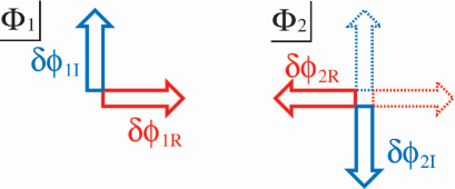
Figure 1: The relative fluctuations between $\Phi_{1}$ and $\Phi_{2}$ (solid arrows), which grows due to the $D$-term instability. The single-field parametrization deals only with the collective fluctuations shown as dotted arrows.

Note that this approximation picks out the relative fluctuations between the constituent fields $\Phi_{1}$ and $\Phi_{2}$, which are disregarded in the single-field parametrization. See Fig. 1. If all the relative fluctuations possessed very heavy masses $\sim g\left\langle\Phi\right\rangle$, the single-field parametrization might suffice. However, one of the relative fluctuations is actually a massless mode as shown below, which experiences the $D$-term instability and thereby grows rapidly.

Hereafter we follow the motion of relative fluctuations $\delta\phi_{R}$ and $\delta\phi_{I}$ defined as

$$\delta\phi_{R} \equiv \frac{\delta\phi_{1R}-\delta\phi_{2R}}{2},$$

$$\delta\phi_{I} \equiv \frac{\delta\phi_{1I}-\delta\phi_{2I}}{2},$$ (20)

and drop the subindices $``1"$ and $``2"$ at the homogeneous fields. The equations of motion for fluctuations $\delta\phi_{R}$ and $\delta\phi_{I}$ are written in the following form:

$$\left(\begin{array}[]{c}\delta\phi_{R}\\ \delta\phi_{I}\end{array}\right)^{\cdot\cdot}+\omega_{k}^{2}\left(\begin{array}[]{c}\delta\phi_{R}\\ \delta\phi_{I}\end{array}\right)=0$$ (25)

with

$$\omega_{k}^{2}\equiv\left(\begin{array}[]{cc}k^{2}+m_{\Phi}^{2}+2g^{2}\phi_{R}^{2}&2g^{2}\phi_{R}\phi_{I}\\ 2g^{2}\phi_{I}\phi_{R}&k^{2}+m_{\Phi}^{2}+2g^{2}\phi_{I}^{2}\end{array}\right).$$ (28)

In order to diagonalize $\omega_{k}^{2}$, we define $R_{k}$ and $\delta\phi_{M,m}$ as

$$\left(\begin{array}[]{c}\delta\phi_{R}\\ \delta\phi_{I}\end{array}\right)=R_{k}\left(\begin{array}[]{c}\delta\phi_{M}\\ \delta\phi_{m}\end{array}\right),~{}~{}~{}R_{k}\equiv\frac{1}{\phi_{o}}\left(\begin{array}[]{cc}\phi_{R}&-\phi_{I}\\ \phi_{I}&\phi_{R}\end{array}\right),$$ (29)

where $\phi_{o}$ is a constant representing the typical amplitude of the flat direction. The eigenvalues of $\omega_{k}^{2}$ corresponding to $\delta\phi_{M}$ and $\delta\phi_{m}$ are $k^{2}+m_{\Phi}^{2}+2g^{2}(\phi_{R}^{2}+\phi_{I}^{2})$ and $k^{2}+m_{\Phi}^{2}$, respectively. Since the frequency of $\delta\phi_{M}$ is much larger than that of the homogeneous motion, its evolution is adiabatic, which means that the particle production of $\delta\phi_{M}$ is negligible. The equation of motion for $\delta\phi_{m}$ is thus given by

$$\delta\ddot{\phi}_{m}-m_{\Phi}(1-\varepsilon^{2})\frac{\sin{2m_{\Phi}t}}{\cos^{2}{m_{\Phi}t}+\varepsilon^{2}\sin^{2}{m_{\Phi}t}}\delta\dot{\phi}_{m}+k^{2}\delta\phi_{m}=0,$$ (30)

where we have substituted the solution for the homogeneous mode:

$$\phi_{R}=\phi_{o}\cos{m_{\Phi}t},$$

$$\phi_{I}=\varepsilon\phi_{o}\sin{m_{\Phi}t},$$ (31)

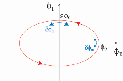
Figure 2: The homogeneous motion and the fluctuation along the elliptical orbit.

and we have neglected $\delta\dot{\phi}_{M}$ in Eq. (30) since it is rapidly oscillating. $\delta\phi_{m}$ is fluctuation along the elliptical orbit as shown in Fig. 2, which can be confirmed by noting that Eq. (30) except for the third term is same as the equation of motion for the angular variable $\theta$ of the homogeneous AD field moving in an elliptic orbit with axial ratio $\varepsilon$:

$$\ddot{\theta}+2\frac{\dot{\phi}}{\phi}\dot{\theta}=0,$$ (32)

where $\phi$ and $\theta$ represent the amplitude and angle of $\Phi$ in the single-field representaion: $\phi^{2}/2=\phi_{R}^{2}+\phi_{I}^{2}$; $\tan\theta=\phi_{I}/\phi_{R}$. Using this analogy, it is easy to see that Eq. (30) contains instabilities, leading to the rapid growth of $\delta\phi_{m}$. Clearly, the angle $\theta$ increases monotonically as the AD field moves around in its orbit. In particular, $\theta$ exhibits step-function-like behavior for $\varepsilon\ll 1$. Therefore we can deduce that $\delta\phi_{m}$ as well increases monotonically aside from the case of $\varepsilon=1$, in which $\delta\phi_{m}$ oscillates with the constant angular frequency $k$, while $\theta$ increases linearly with time.

To see the band structure of this instability, let us rewrite this equation in terms of $\tau$ and $\delta\varphi$ defined as

$$\tau \equiv m_{\Phi}t-\frac{\pi}{2},$$ (33)

$$\delta\varphi \equiv \delta\phi_{m}\sqrt{1+\varepsilon^{2}-(1-\varepsilon^{2})\cos{2\tau}}.$$ (34)

Then we obtain the final result:

$$\delta\varphi^{{}^{\prime\prime}}+\left(\frac{k^{2}}{m_{\Phi}^{2}}+F(\varepsilon,\tau)\right)\delta\varphi=0$$ (35)

with

$$F(\varepsilon,\tau)\equiv\frac{(1-\varepsilon^{2})(\sin^{4}{\tau}-\varepsilon^{2}\cos^{4}{\tau})}{(\sin^{2}{\tau}+\varepsilon^{2}\cos^{2}{\tau})^{2}},$$ (36)

where the prime denotes the differentiation with respect to $\tau$. It is worth noting that the amplitude of the flat direction $\phi_{o}$ disappears in the Eqs. (30) and (35). Therefore the instability band and exponential growth rate are independent of the amplitude.

First let us take the limit of $\varepsilon\rightarrow 1$ in Eq. (35). It then reduces to the well-known Mathieu equation mathieu :

$$\delta\varphi^{{}^{\prime\prime}}+(A-2q\cos{2\tau})\delta\varphi=0$$ (37)

with $A=k^{2}/m_{\Phi}^{2}$ and vanishingly small $q$-parameter $q\simeq 1-\varepsilon$. For $q\ll 1$, the resonance is known to occur only in narrow bands near $A=l^{2}$, $(l=1,2,\dots)$, and the instability vanishes if $q=0$. Therefore we expect that the nature of the instabilities of Eq. (35) is similar to that of the Mathieu equation, if the AD field is rotating in a roughly circular orbit. That is to say, the narrow-band resonance occurs around $k/m_{\Phi}=l$, $(l=1,2,\dots)$, and $\delta\varphi$ grows unless the flat direction is moving in an exact circular orbit (i.e., $q=1-\varepsilon=0$). The instability chart of Eq. (35) is illustrated in Fig. 3, and one can see that the narrow-band structure around $\varepsilon=1$ resembles those of the Mathieu equation.

Next we take up the other limit of $\varepsilon\ll 1$. In this case, the function $F(\varepsilon,\tau)$ behaves as follows. For $|\tau|\lesssim\varepsilon^{-1/2}$, it becomes negative and the minimum locates at $\tau=0$: $F(\varepsilon,0)=-\varepsilon^{-2}$, while $F(\varepsilon,\tau)\simeq 1$ for $|\tau|\gtrsim\varepsilon^{-1/2}$. See Fig. 4. Therefore those fluctuations with $k<\varepsilon^{-1}m_{\Phi}$ experience tachyonic instabilities and grow exponentially each time $\tau$ passes $\tau=n\pi,~{}(n=0,1,2,\dots)$. That is to say, the instability shows the step-function-like behavior, as expected. As can be seen from Fig. 3, the instabilities become stronger for smaller $\varepsilon$. However we expect that the exponential growth rate will converge to some finite value $\sim O(1)$ as $\varepsilon\rightarrow 0$.

So far we have neglected the cosmic expansion, but the above-mentioned nature of the instability does not change much even if the cosmic expansion is taken into consideration. For simplicity, let us assume that the universe is dominated by the energy of the oscillating inflaton, when the AD field starts to oscillate (i.e., $H\simeq m_{\Phi}$). Then similar arguments lead to the equation of motion of $\delta\phi_{m}$ given by Eq. (30) with $k^{2}$ replaced with $k^{2}/a^{2}$, where $a$ denotes the scale factor. Note that the solution of the homogeneous mode is now given by

$$\phi_{R}=\phi_{o}a^{-3/2}\cos{m_{\Phi}t},$$

$$\phi_{I}=\varepsilon\phi_{o}a^{-3/2}\sin{m_{\Phi}t}.$$ (38)

Due to the redshift of the momentum $k$, the band structure becomes vague as seen in Fig. 5. However, except for $\varepsilon\sim 1$ where the instability is narrow-band resonance, there still exist strong $D$-term instabilities because of their tachyonic nature.

The above argument is not limited to the parabolic potential, but it can easily be generalized to an arbitrary potential with $U(1)$ symmetry. Although the collective fluctuations as well are subject to instabilities peculiar to the potential in general, we can concentrate on the relative fluctuations by adopting Eq. (19) since they are independent. As long as the homogeneous motion satisfies the $D$-flat condition, the lighter one of the relative fluctuations satisfies

$$\delta\ddot{\phi}_{m}+2\frac{\dot{\phi}}{\phi}\delta\dot{\phi}_{m}+k^{2}\delta\phi_{m}=0,$$ (39)

where the definitions of the variables are same as before. If we rewrite this equation in terms of $\delta\varphi\equiv\phi\,\delta\phi_{m}$, we have

$$\delta\ddot{\varphi}+\left(k^{2}-\frac{\ddot{\phi}}{\phi}\right)\delta\varphi=0.$$ (40)

When the AD field comes the closest to the origin, $\ddot{\phi}/\phi$ is expected to take its maximum value, which leads to the tachyonic instabilities for $k^{2}<[\ddot{\phi}/\phi]_{\rm max}$. Also if the homogeneous motion in the limit of $\varepsilon\rightarrow 1$ can be approximated as

$$\phi_{R}=\phi_{o}\cos{\Omega t},$$

$$\phi_{I}=\varepsilon\phi_{o}\sin{\Omega t},$$ (41)

then Eq. (40) reduces to the Mathieu equation with $A=k^{2}$ and $q\simeq\Omega^{2}(1-\varepsilon)$. In this case, the instability bands are narrow and locate at $k/\Omega=l,~{}(l=1,2,\dots)$. Thus the existence of the $D$-term instability does not depend on the specific form of the potential.

In this section we have considered a simple model of $D$-flat directions. However the existence of the instability should be common to all $D$-flat directions. The reason is as follows. First, all the MSSM flat direction is at least charged under $U(1)_{Y}$. Thus $D$-term potential similar to Eq. (13) always exists. Second, the instability originates from a massless mode of the relative fluctuations between the constituent fields, the existence of which is a common feature of $D$-flat directions. To sum up the major characteristics of the $D$-term instability, (i) for $\varepsilon\sim 1$, it is narrow-band resonance similar to the one expresssed by the Mathieu equation; (ii) the tachyonic instability appears for $\varepsilon<1$; (iii) it is independent of amplitude of the flat direction. In the following sections we will see how such $D$-term instability affects the dynamics of the AD field.

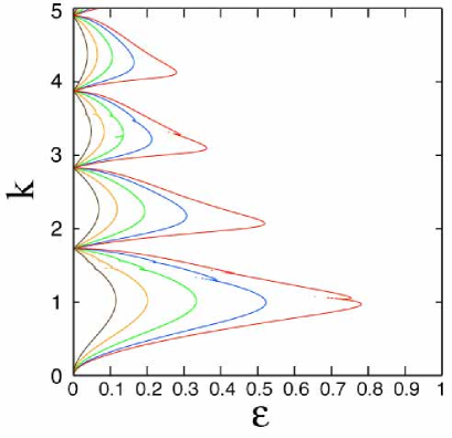
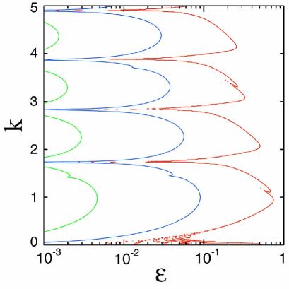
Figure 3: The instability charts of Eq. (35). The momentum $k$ is normalized by $m_{\Phi}$. The left and right panels are equivalent except for the plotted range of $\varepsilon$. Each contour line corresponds to $\mu/m_{\Phi}=0.1,0.3,0.5,0.7,0.9$ from right to left in the left panel, while $\mu/m_{\Phi}=0.1,1,2$ from right to left in the right panel, where $\mu$ is an exponential growth rate of fluctuations.

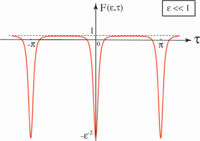
Figure 4: The typical behavior of $F(\varepsilon,\tau)$ when $\varepsilon\ll 1$.

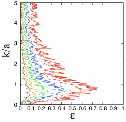
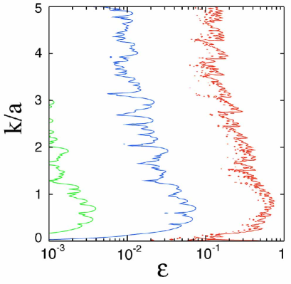
Figure 5: Same as Fig. 3 except that the cosmic expansion is taken into account. We take the initial condition as $H=m_{\Phi}$, and assumed the matted-dominated like universe.

III Effects on $Q$-ball formation

III.1 Review of $Q$-balls and $I$-balls

Let us now discuss how the $D$-term instability affects the $Q$-ball formation processes. Before we go into details, it will be useful to briefly review the $Q$-ball formation. For the moment we adopt the single-field parametrization. Let a flat direction $\Phi$ possess an unit baryon charge. During inflation $\Phi$ is assumed to take a large expectation value. When the Hubble parameter becomes comparable to the mass of $\Phi$ after inflation ends, $\Phi$ starts to oscillate in the potential Eq. (7). If the sign of $K$ is negative, it experiences spatial instabilities, leading to the $Q$-ball formation Kusenko:1997si ; Enqvist:1998en ; Kasuya:1999wu . The profile of thus formed gravity-mediation type $Q$-balls is approximated by the spherically symmetric gaussian form with good precision: Enqvist:1998en

$$\Phi = \frac{\phi_{R}+i\phi_{I}}{\sqrt{2}},$$

$$\phi_{R}(r,t) = \phi_{o}\,e^{-r^{2}/R_{Q}^{2}}\cos{\omega t},$$

$$\phi_{I}(r,t) = \phi_{o}\,e^{-r^{2}/R_{Q}^{2}}\sin{\omega t},$$ (42)

with

$$\omega \equiv m_{\Phi}\sqrt{1+2|K|},$$

$$R_{Q} \equiv \frac{\sqrt{2}}{\sqrt{|K|}m_{\Phi}},$$ (43)

where $\omega$ and $R_{Q}$ denote the angular velocity and radius of the $Q$-ball, respectively.

Although a $Q$-ball solution is realized as the energy minimum state with a fixed global $U(1)$ charge, it is a $I$-ball that is first formed in general. The profile of $I$-balls is almost same as that of $Q$-balls except for axial ratio of the orbit:

$$\phi_{R}(r,t) = \phi_{o}\,e^{-r^{2}/R_{Q}^{2}}\cos{\omega t},$$

$$\phi_{I}(r,t) = \varepsilon_{I}\,\phi_{o}\,e^{-r^{2}/R_{Q}^{2}}\sin{\omega t},~{}~{}~{}(0\leq\varepsilon_{I}<1).$$ (44)

The reason why $I$-balls are formed instead of $Q$-balls is that the quadratic potential Eq. (7) allows the dynamics of system to have another invariant, the adiabatic charge $I$ Kasuya:2002zs , and that the axial ratio of the homogeneous motion is generally less than $1$. Thanks to the conservation of the adiabatic charge, $I$-balls are formed as a quasi-stable state, and the axial ratio of the orbit inside $I$-balls, $\varepsilon_{I}$, is almost same as that of homogeneous mode before fluctuations grow, $\varepsilon_{H}$:

$$\varepsilon_{I}\simeq\varepsilon_{H}.$$

However this relation does not hold when the $D$-term instability is taken into account, and $\varepsilon_{I}$ is larger than or equal to $\varepsilon_{H}$ as shown below.

Central to this issue is how $I$-balls eventually transform into $Q$-balls. Due to the elliptical orbit, $I$-balls are considered to be an excited state of $Q$-balls. However it was unclear to date how $I$-balls emit the extra energy to settle down to $Q$-balls, since they have very long lifetime, which makes it difficult to follow the evolution in numerical calculations. Here we would like to argue that the $D$-term instability violates the conservation of the adiabatic charge, which enables $I$-balls, if formed, to immediately transform into $Q$-balls by emitting both the energy and $U(1)$ charge.

Before we proceed, however, it is necessary to ask whether $I$-balls are really formed under the influence of the $D$-term instabilities. Since the exponential growth rate of the $I$-ball formation is given by $\mu_{Q}\sim|K|m_{\Phi}\sim 0.1m_{\Phi}$ Enqvist:1998en , the $I$-ball formation will complete before the $D$-term instabilities grow sufficiently, if the initial axial ratio $\varepsilon_{H}$ is larger than $\sim 0.7$ (see Fig. 5). Furthermore, even if the $D$-term instabilities grows faster than $\sim|K|m$, some $I$-ball-like objects might be generated as a result of the interactions between the developed fluctuations, because the fastest growing mode of the $D$-term instability locates around $k/a\sim m_{\Phi}$ which is not so different from the typical size of $I$-balls. In fact, we have performed numerical calculations not taking account of the cosmic expansion and confirmed that $I$-balls are formed for $\varepsilon_{H}\geq 0.1$, but the axial ratio of the orbit inside thus formed lumps is larger than $\varepsilon_{H}$ from the beginning, e.g., $\varepsilon_{I}\sim 0.3$ for $\varepsilon_{H}=0.1$. In particular, $I$-balls with $\varepsilon_{I}\lesssim 0.2$ are not formed, probably because the $D$-term instability with $\varepsilon_{I}\lesssim 0.2$ is too strong for $I$-balls to retain their configuration. Although the cosmic expansion might make the interactions between the fluctuations less effective, some part of the charge asymmetry will still be stored inside such $I$-ball-like objects. We will discuss the evolution of the axial ratio of the trajectory inside these objects in the next two subsections.

The $I$-ball formation is not the end of the story. Once $I$-balls are formed, the dynamics of the AD field inside them decouples from the cosmic expansion. Since the $D$-term instabilities lie at smaller scales than a typical size of $I$-balls, fluctuations inside them continue to grow exponentially. It should be noted that the $D$-term instability does not depend on the amplitude, so that they will grow throughout the $I$-ball. The growth will last either until the conversion of $I$-balls into $Q$-balls completes (i.e., the axial ratio $\varepsilon$ becomes 1), or until $I$-balls are completely destroyed by the instability. We need to resort to numerical calculations to determine which is realized.

III.2 Numerical Calculations

As mentioned in the previous subsection, we have numerically investigated the formation processes of $I$-balls taking account of the $D$-term instability and found that almost all the charge asymmetry is taken in the $I$-balls for $\varepsilon_{H,{\rm ini}}\geq 0.1$:

$$f_{I}\simeq 1,$$ (45)

where $f_{I}$ denotes the fraction of the charge absorbed by the $I$-balls. Due to the technical reasons, it is difficult both to take account of the cosmic expansion and to follow the evolution of the AD field with $\varepsilon_{H,{\rm ini}}\leq 0.1$. The cosmic expansion might change the $I$-ball formation inefficient to some extent. The strong instability for $\varepsilon_{H,{\rm ini}}\ll 0.1$ as well prevents the $I$-balls to be formed. But what we would like to show here is that the charge asymmetry is partly left behind during the $Q$-ball formation, even if it is once absorbed by $I$-balls.

Assuming that $I$-balls are formed, we have followed the evolution of the $I$-ball in order to show that the $D$-term instability actually occurs inside $I$-balls. We have solved the equations of motion given by Eq. (12) on the one dimensional lattices with the initial condition:

$$\phi_{1R}=\phi_{2R} = \phi_{o}\,e^{-r^{2}/R_{Q}^{2}}\cos{m_{\Phi}t},$$

$$\phi_{1I}=\phi_{2I} = \varepsilon_{I}\,\phi_{o}\,e^{-r^{2}/R_{Q}^{2}}\sin{m_{\Phi}t}.$$ (46)

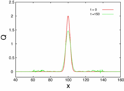
Figure 7: Spatial distributions of energy and charge of the $I$-ball with the initial axial ratio: $\varepsilon_{I}=0.5$. The $I$-ball becomes more $Q$-ball-like by emitting both the energy and the charge. Note that the energy is more efficiently released than the charge, which makes the effective axial ratio increase.

Once $I$-balls are formed, the dynamics inside them decouples from the cosmic expansion. Therefore we can safely neglect the effect in contrary to the case before the $I$-balls are formed. It should be reminded that the axial ratio $\varepsilon_{I}$ in the above equation does not necessarily coincides with that of the homogeneous motion $\varepsilon_{H}$. The space $x$ and time $t$ are normalized by the mass scale $m_{\Phi}$, while the field value is normalized by $M_{*}$. We take the following values for the model parameters: $m_{1}=m_{2}=m_{\Phi}$, $\phi_{o}/M_{*}=1$, $g^{2}M_{*}^{2}=10^{3}~{}{\rm or~{}}10^{4}\,m_{\Phi}^{2}$, and $K_{1}=K_{2}=-0.1$. The typical evolution of the axial ratio $\varepsilon_{I}$ with the initial value: $\varepsilon_{I}=0.5$, is illustrated in Fig. 6. The spatial distributions of the energy and the charge are shown in Fig. 7. As seen in the figure, the axial ratio increases, but it does not reach $1$ due to the following reasons. First of all, as the axial ratio comes closer to $1$, the instability becomes weaker as shown in Fig. 3. Thus in the finite CPU time the complete conversion of the $I$-ball to a $Q$-ball cannot be seen. Second, the finite lattice size allows the decay product emitted from the $I$-ball to be absorbed by the $I$-ball again. This effect as well prevents the $I$-ball to transform into the $Q$-ball. (We have chosen the time interval in Fig. 6, so that this effect is negligible.) However, in the real world, such a tendency toward $Q$-balls will last throughout, because the adiabatic charge is no longer conserved due to the $D$-term instability. We thus expect the conversion will be completed relatively soon after the $I$-ball formation.

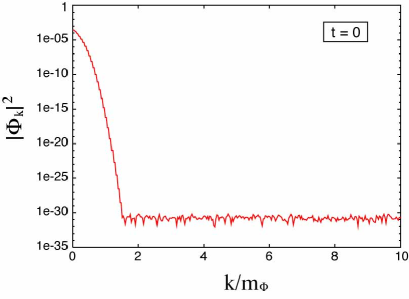
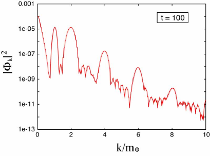
Figure 8: Power spectra of the constituent field $\Phi_{1}$. The model parameters are same as before except $K_{1}=K_{2}=-0.01$. The upper panel represents the power spectrum of the initial $I$-ball solution with $\varepsilon_{I}=0.5$, while the $D$-term instability begins to grow in the lower panel. The instability bands coincide with those obtained by the analysis of linearized fluctuations (see Fig. 3). The instability bands corresponding to $k/m_{\Phi}=2,4,6,\dots$ are enhanced due to“rescattering” processes.

We have also calculated the power spectra of one of the constituent fields, $\Phi_{1}$. See Fig. 8. We take the size of the $I$-ball larger (i.e., smaller $|K|$) to obtain clear signature of the instability band. The result coincides with the instability band obtained by the analysis of linearized fluctuations. Thus we conclude that the $D$-term instability plays an essential role to transform $I$-balls into $Q$-balls.

III.3 Modified relation between baryon and dark matter abundance

What should be emphasized at this juncture is that both the energy and charge are emitted from the $I$-ball. This is because the four-point interaction in the $D$-term inevitably induces both the charge-transferring (e.g., $\Phi_{1}\Phi_{1}\rightarrow\Phi_{1}\Phi_{1}$) and charge-conserving processes (e.g., $\Phi_{1}\Phi_{1}^{*}\rightarrow\Phi_{1}\Phi_{1}^{*}$). If almost all the charge is absorbed by the $I$-balls at their formation, the fraction of the baryon charge stored inside $Q$-balls, $f_{Q}$, depends only on the initial axial ratio . Since $f_{Q}$ is defined as the fraction of the charge stored inside $Q$-balls assuming all the charge asymmetry is once absorbed by $I$-balls, the actual fraction kept inside $Q$-balls is $f_{B}\equiv f_{I}f_{Q}$. It is important to know the value of $f_{B}$ to relate the baryon number to dark matter density. The numerical results of $f_{Q}$ for several values of $\varepsilon_{I}$ are summarized in Table 1. The values of $f_{Q}$ shown in the table should be considered to give upper bounds of $f_{B}$, since some part of the charge is left behind at the $I$-ball formation and also the conversion is not yet completed. It should be noted that the $I$-ball comes apart for $\varepsilon_{I}\leq 0.2$ due to the strong $D$-term instability. This fact agrees with the result that $I$-balls with the axial ratio smaller than $\sim 0.2$ are not formed.

The neutralino LSPs produced by the decay of $Q$-balls survive and can be the dark matter, if the decay temperature of $Q$-balls is lower than the freeze-out temperature of the LSP. Let $N$ be the average number of the LSPs produced by the decay of unit baryon charge of $Q$-balls. The abundance of the LSP dark matter is then related to that of baryon number as follows.

$$\Omega_{DM}=3\left(\frac{N}{3}\right)\left(\frac{m_{\rm LSP}}{m_{n}}\right)f_{B}\Omega_{B},$$ (47)

where $\Omega_{DM,\,B}$ denote the density parameters of the dark matter and the baryon, $m_{\rm LSP}$ and $m_{n}$ are masses of the LSP and the nucleon, respectively. Substituting the WMAP results Spergel:2003cb : $\Omega_{DM}h^{2}=0.116$ and $\Omega_{B}h^{2}=0.024$, we obtain

$$f_{B}\sim 0.02\left(\frac{3}{N}\right)\left(\frac{m_{\rm LSP}}{100{\rm GeV}}\right)^{-1}$$ (48)

Previously, $f_{B}\sim 1$ was supported by the numerical calculations Kasuya:2000wx , therefore the coincidence of the baryon and dark matter abundance cannot be explained in this way. However, thanks to the $D$-term instability, $f_{I}\ll 1$ might be achieved if $\varepsilon_{H}$ is much less than $\sim 0.1$. Since the flat direction completely decays before $I$-balls are formed for small enough $\varepsilon_{H}$, there must be an intermediate value of $\varepsilon_{H}$ that leads to $f_{B}\sim 0.02$.

On the other hand, the new-type $Q$-balls Kasuya:2000sc themselves can be the dark matter in the gauge-mediated SUSY breaking models. Since the new-type $Q$-balls are formed where the gravity-mediated potential overwhelms the gauge-mediated one, the above-mentioned arguments can be applied. If the energy per unit charge of the new-type $Q$-ball is smaller than the nucleon mass, they are stable and can be the dark matter. The relation between the dark matter and the baryon abundance is thus given by

$$\Omega_{DM}=\frac{f_{B}}{1-f_{B}}\frac{m_{3/2}}{m_{n}}\Omega_{B},$$ (49)

where we take $m_{\Phi}\simeq m_{3/2}$. This gives the constraint on $f_{B}$:

$$f_{B} = \frac{\Omega_{DM}}{\Omega_{DM}+\frac{m_{3/2}}{m_{n}}\Omega_{B}},$$ (50)

$$\simeq 1.0,~{}0.98,~{}0.83,~{}~{}~{}~{}{\rm for~{}~{}}m_{3/2}=0.01,~{}0.1,~{}1{\rm GeV},$$

which can be explained by taking e.g., $\varepsilon_{H}\gtrsim 0.4$ if $f_{I}\simeq 1$ and $\varepsilon_{H}\simeq\varepsilon_{I}$.

It has been thought that almost all the baryon number is absorbed in $Q$-balls. That is why it was necessary to estimate how much the baryon charge evaporates from the surface of $Q$-balls through the interaction with thermal plasma. However, in fact, some finite fraction is emitted from $I$-balls due to the $D$-term instability, and the fraction is determined only by the initial axial ratio, independent of the reheating temperature and so on. Thus the $D$-term instability may revive the appealing solution for the coincidence problem between the dark matter and baryon abundance, which was otherwise difficult to be achieved.

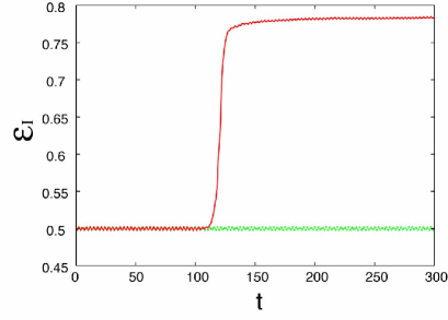
Figure 6: Evolutions of the axial ratio of the orbit inside a $I$-ball with the initial value:$\varepsilon_{I}=0.5$. Due to the $D$-term instability, $\varepsilon_{I}$ tends to approach $1$ (solid line), while it remains constant in the single-field parametrization (dotted line).

Table 1: Numerical results of the final axial ratio and $f_{Q}$. For $\varepsilon_{I}\leq 0.2$, the $I$-ball divides into mutliple $Q$-balls, and the final axial ratio and $f_{Q}$ of the largest one are shown in parenthesis below. For $\varepsilon_{I}=0.9$, the conversion of the $I$-ball to a $Q$-ball cannot be observed in the numerical calculation.

$\varepsilon_{I,{\rm ini}}$	0.1	0.2	0.3	0.4	0.5	0.6	0.7	0.8	0.9
$\varepsilon_{I,{\rm fin}}$	(0.5)	(0.6)	0.7	0.73	0.78	0.8	0.82	0.85	0.9
$f_{Q}$	(0.15)	(0.6)	0.72	0.85	0.93	0.96	0.97	0.99	1.0

IV Fate of flat directions

In the previous section we have considered the case that $Q$-balls are formed. What if $Q$-balls are not formed? If the coefficient of the one-loop correction $K$ is positive, $Q$-balls are not formed. Also even if $K$ is negative, the strong tachyonic instabilities will prevent $Q$-balls from being formed, when the initial axial ratio is small enough. It should be noted that $Q$-balls remain stable under the effect of the $D$-term instability since the instability disappears when the orbit becomes circular. In other words, unless $Q$-balls are formed, the $D$-term instability will never cease to grow. Therefore, if $K<0$ or $K>0$ with $\varepsilon_{H}\ll 1$, the flat direction experiences the $D$-term instability until it deforms into a disordered state, which will decay and/or interact with other particles and attain the thermal equilibrium sooner or later. The fate of the flat directions is thus very simple: $Q$-ball or nothing.

From the above discussion, the gravity-mediation type $Q$-balls are formed when the initial axial ratio of the orbit is large enough $\varepsilon_{H}\gtrsim 0.1$. Then what about the gauge-mediation type $Q$-balls? Since the strength of the $A$-term is proportional to the gravitino mass, the initial axial ratio tends to be much smaller than $1$ if the AD field start to oscillate in the gauge-mediated potential deGouvea:1997tn . Since the homogeneous motion in the gauge-mediated potential cannot be solved analytically, it is necessary to perform numerical calculations to investigate the $D$-term instabilities. Due to this additional instability, the $Q$-ball formation will be considerably delayed or prevented. The detailed discussion on this subject will be presented elsewhere preparation .

V discussions

In this paper we have investigated the dynamics of the flat directions taking account of the $D$-term potential. To this end, we adopted the multi-field parametrization of the flat directions, which enables us to deal with the relative fluctuations between the constituent fields. It is found that there exist instabilities due to the D-term potential and the nature of these instabilities depends on the axial ratio $\varepsilon$ of the oscillating flat direction. If $\varepsilon$ is close to $1$, the $D$-term instability is similar to narrow resonance described by the Mathieu equation with $q\ll 1$. On the other hand, the instabilities show the tachyonic nature for $\varepsilon<1$. Due to this tachyonic instability, the cosmological evolution of the flat direction are always under the influence of $D$-term instability. In particular we have shown that the existence of the instabilities is crucial to the formation of $Q$-balls. Since the $D$-term instability violates the conservation of the adiabatic charge, $I$-balls are no longer quasi-stable, and therefore the transition from $I$-balls to $Q$-balls occurs very efficiently. It is important to note that during this process some fraction of the charge of the $Q$-ball is emitted, which may revive the relation between the baryon number and dark matter density of the universe. Furthermore, the $D$-term instability drastically changes the evolution of the flat directions. Unless $Q$-balls are formed, the flat direction completely decays relatively soon after it begins to oscillate. We believe that the existence of such instabilities is generic to the system of scalar fields with the $D$-term potential. For instance, in the reheating stage of the $D$-term inflation models Binetruy:1996xj , the scalar fields are oscillating in the similar potential. Thus the reheating processes of inflation models of this type might be affected by the $D$-term instability. However, further investigation is clearly necessary and is beyond the scope of this paper.

ACKNOWLEDGMENTS

We would like to thank S. Kasuya for reading the manuscript and useful comments. F.T. would like to thank the Japan Society for the Promotion of Science for financial support. This work was partially supported by the JSPS Grant-in-Aid for Scientific Research No. 14540245 (M.K.).

References

- (1) I. Affleck and M. Dine, Nucl. Phys. B 249, 361 (1985); M. Dine, L. Randall and S. Thomas, Nucl. Phys. B 458, 291 (1996) [arXiv:hep-ph/9507453].
- (2) S. R. Coleman, Nucl. Phys. B 262, 263 (1985) [Erratum-ibid. B 269, 744 (1986)].
- (3) A. Kusenko and M. E. Shaposhnikov, Phys. Lett. B 418, 46 (1998) [arXiv:hep-ph/9709492].
- (4) K. Enqvist and J. McDonald, Nucl. Phys. B 538, 321 (1999) [arXiv:hep-ph/9803380].
- (5) S. Kasuya and M. Kawasaki, Phys. Rev. D 61, 041301 (2000) [arXiv:hep-ph/9909509].
- (6) S. Kasuya and M. Kawasaki, Phys. Rev. D 62, 023512 (2000) [arXiv:hep-ph/0002285].
- (7) S. Kasuya and M. Kawasaki, Phys. Rev. Lett. 85, 2677 (2000) [arXiv:hep-ph/0006128].
- (8) S. Kasuya and M. Kawasaki, Phys. Rev. D 64, 123515 (2001) [arXiv:hep-ph/0106119].
- (9) M. Kawasaki, F. Takahashi and M. Yamaguchi, Phys. Rev. D 66, 043516 (2002) [arXiv:hep-ph/0205101].
- (10) K. Ichikawa, M. Kawasaki and F. Takahashi, arXiv:astro-ph/0402522.
- (11) M. Kawasaki and F. Takahashi, arXiv:hep-ph/0403199.
- (12) S. Kasuya, M. Kawasaki and F. Takahashi, Phys. Lett. B 559, 99 (2003) [arXiv:hep-ph/0209358].
- (13) T. Chiba, F. Takahashi and M. Yamaguchi, Phys. Rev. Lett. 92, 011301 (2004) [arXiv:hep-ph/0304102]; F. Takahashi and M. Yamaguchi, Phys. Rev. D 69, 083506 (2004) [arXiv:hep-ph/0308173].
- (14) L. Kofman, A. D. Linde and A. A. Starobinsky, Phys. Rev. D 56, 3258 (1997) [arXiv:hep-ph/9704452]; P. B. Greene, L. Kofman, A. D. Linde and A. A. Starobinsky, Phys. Rev. D 56, 6175 (1997) [arXiv:hep-ph/9705347].
- (15) G. N. Felder, L. Kofman and A. D. Linde, Phys. Rev. D 59, 123523 (1999) [arXiv:hep-ph/9812289].
- (16) S. Kasuya, T. Moroi and F. Takahashi, arXiv:hep-ph/0312094.
- (17) N. W. Mac Lachlan, Theory and Application of Mathieu Functions (Dover, New York, 1961).
- (18) D. N. Spergel et al., Astrophys. J. Suppl. 148, 175 (2003) [arXiv:astro-ph/0302209].
- (19) A. de Gouvea, T. Moroi and H. Murayama, Phys. Rev. D 56, 1281 (1997) [arXiv:hep-ph/9701244].
- (20) S. Kasuya, M. Kawasaki and F. Takahashi, in preparation.
- (21) P. Binetruy and G. R. Dvali, Phys. Lett. B 388, 241 (1996) [arXiv:hep-ph/9606342]; E. Halyo, Phys. Lett. B 387, 43 (1996) [arXiv:hep-ph/9606423].