Effective Lagrangian for $\chi^{+}_{i}\chi_{j}^{0}H^{-}$ Interaction in the MSSM and Charged Higgs Decays

Tarek Ibrahim^a,b, Pran Nath^b and Anastasios Psinas ^b

a. Department of Physics, Faculty of Science, University of Alexandria,
Alexandria, Egypt
b. Department of Physics, Northeastern University, Boston, MA 02115-5000, USA

Abstract

We extend previous analyses of the supersymmetric loop correction to the charged Higgs couplings to include the coupling $H^{\pm}\chi^{\mp}\chi^{0}$. The analysis completes the previous analyses where similar corrections were computed for $H^{+}\bar{t}b$ ($H^{-}t\bar{b}$), and for $H^{+}\tau^{-}\bar{\nu}_{\tau}$ ($H^{-}\tau^{+}\nu_{\tau}$) couplings within the minimal supersymmetric standard model. The effective one loop Lagrangian is then applied to the computation of the charged Higgs decays. The sizes of the supersymmetric loop correction on branching ratios of the charged Higgs $H^{+}(H^{-})$ into the decay modes $t\bar{b}$ ($\bar{t}b$), $\bar{\tau}\nu_{\tau}$ ($\tau\bar{\nu}_{\tau}$), and $\chi_{i}^{+}\chi_{j}^{0}(\chi_{i}^{-}\chi_{j}^{0})$ (i=1,2; j=1-4) are investigated and the supersymmetric loop correction is found to be significant, i.e., in the range 20-30% in significant regions of the parameter space. The loop correction to the decay mode $\chi_{1}^{\pm}\chi_{2}^{0}$ is examined in specific detail as this decay mode leads to a trileptonic signal. The effects of CP phases on the branching ratio are also investigated. A brief discussion of the implications of the analysis for collders is given.

1 Introduction

The Higgs couplings to matter and to gauge fields are of great current interest as they enter in a variety of phenomena which are testable in low energy processes[1]. Specifically it has been known for some time that the loop correction to the b quark mass generates a contribution which becomes large for large $\tan\beta$ underlining the importance of the loop correction in phenomena involving the Higgs boson couplings[2]. Recently analyses of the supersymmetric one loop corrections to the Higgs boson couplings were given and its implications for the decay of the Higgs into $H^{+}\rightarrow t\bar{b}$ ($H^{-}\rightarrow\bar{t}b$) and $H^{+}\rightarrow\bar{\tau}\nu_{\tau}$ ($H^{-}\rightarrow\tau\bar{\nu}_{\tau}$) were analysed[3, 4, 5, 6, 7] . These decays are of great importance as they differ strongly from the predictions in the Higgs sector of the Standard Model and thus provide possible signals for the observation of supersymmetry at colliders. In the analysis given in Refs.[4, 5, 6, 7] the decay of the Higgs into chargino and neutralinos was, however, not considered. In this paper we extend the analysis to include the loop correction to the $H^{\pm}\chi^{\mp}\chi^{0}$ couplings. We also take into account the effects of the CP phases.

The analysis is carried out in the framework of the minimal supersymmetric standard model (MSSM). For the numerical part of the analysis we work within the framework of extended supergravity unified models. Thus the mimimal supergravity unified model (mSUGRA)[8] is parametrized by the universal scalar mass $m_{0}$, the universal gaugino mass $m_{\frac{1}{2}}$, the universal trilinear coupling $A_{0}$, the ratio of the Higgs vacuum expectation values (VEVs), i.e., $\tan\beta=<H_{2}>/<H_{1}>$ where $H_{2}$ gives mass to the up quark and $H_{1}$ gives VEV to the down quark and the lepton, and sign($\mu)$) where $\mu$ is the Higgs mixing parameter which appears in the superpotential in the form $\mu H_{1}H_{2}$. mSUGRA is based on the assumption of a flat Kahler potential and thus can be extended by inclusion of more general Kahler potentials. This allows one to introduce nonuniversalities in the soft parameters. Thus for more general analyses,we will assume nonuniversalities in the Higgs sector, and also allow for CP phases. The inclusion of phases of course involves attention to the severe experimental constraints that exist on the electric dipole moment (edm) of the electron[9], of the neutron[10] and of ${}^{199}Hg$ atom[11]. However, as is now well known there are a variety of techniques available that allow one to suppress the large edms and bring them in conformity with the current experiment[12, 13, 14, 15]. CP phases affect loop corrections to the Higgs mass[16], dark matter[17] and a number of other phenomena (for a review see Ref.[18]). The outline of the rest of the paper is as follows: In Sec.2 we compute the loop correction to the $H^{\pm}\chi^{\mp}\chi^{0}$ couplings arising from supersymmtric particle exchanges and the effects of these corrections on the charged Higgs decay. In Sec.3 we give a numerical analysis of the sizes of radiative corrections. It is found that the loop correction can be as large as 25-30% in certain parts of the parameters space. Implications of these results at colliders are briefly discussed in Sec.4 and conclusions are given in Sec.5.

2 Loop Corrections to Charged Higgs Couplings

The microscopic Lagrangian for $H^{\pm}\chi^{\mp}\chi^{0}$ interaction is

$${\cal{L}}=\xi_{ji}H_{2}^{1*}\bar{\chi}_{j}^{0}P_{L}\chi_{i}^{+}+\xi_{ji}^{\prime}H_{1}^{2}\bar{\chi}_{j}^{0}P_{R}\chi_{i}^{+}+H.c.$$ (1)

where $H_{1}^{2}$ and $H_{2}^{1}$ are the charged states of the two Higgs iso-doublets in the minimal supersymmetric standard model (MSSM), .i.e,

$$(H_{1})=\left(\matrix{H_{1}^{1}\cr H_{1}^{2}}\right),~{}~{}(H_{2})=\left(\matrix{H_{2}^{1}\cr H_{2}^{2}}\right)$$ (2)

and $\xi_{ji}$ and $\xi_{ji}^{\prime}$ are given by

$$\xi_{ji}=-gX_{4j}V_{i1}^{*}-\frac{g}{\sqrt{2}}X_{2j}V_{i2}^{*}-\frac{g}{\sqrt{2}}\tan\theta_{W}X_{1j}V_{i2}^{*}$$ (3)

and

$$\xi_{ji}^{\prime}=-gX_{3j}^{*}U_{i1}+\frac{g}{\sqrt{2}}X_{2j}^{*}U_{i2}+\frac{g}{\sqrt{2}}\tan\theta_{W}X_{1j}^{*}U_{i2}$$ (4)

where $X$, $U$ and $V$ diagonalize the neutralino and chargino mass matrices so that

$$X^{T}M_{\chi^{0}}X=diag(m_{\chi_{1}^{0}},m_{\chi_{2}^{0}},m_{\chi_{3}^{0}},m_{\chi_{4}^{0}})$$

$$U^{*}M_{\chi^{+}}V^{-1}=diag(m_{\chi_{1}^{+}},m_{\chi_{2}^{+}})$$ (5)

where $m_{\chi_{i}^{0}}$ (i=1,2,3,4) are the eigen values of the neutralino mass matrix $M_{\chi^{0}}$ and $m_{\chi_{1}^{+}},m_{\chi_{2}^{+}}$ are the eigen values of the chargino mass matrix $M_{\chi^{+}}$.

The loop corrections produce shifts in the couplings of Eq. (1) and the effective Lagrangian with loop corrected couplings is given by

$${\cal{L}}_{eff}=(\xi_{ji}+\delta\xi_{ji})H_{2}^{1*}\bar{\chi}_{j}^{0}P_{L}\chi_{i}^{+}+\Delta\xi_{ji}H_{1}^{2}\bar{\chi}_{j}^{0}P_{L}\chi_{i}^{+}$$

$$+(\xi_{ji}^{\prime}+\delta\xi_{ji}^{\prime})H_{1}^{2}\bar{\chi}_{j}^{0}P_{R}\chi_{i}^{+}+\Delta\xi_{ji}^{\prime}H_{2}^{1*}\bar{\chi}_{j}^{0}P_{R}\chi_{i}^{+}+H.c.$$ (6)

In this work we calculate the loop correction to the $\chi^{\pm}\chi^{0}H^{\mp}$ using the zero external momentum approximation.

Figure 1: The stop and sbottom exchange contributions to the $H^{-}\chi^{+}\chi^{0}$ vertex.

2.1 Loop analysis of $\Delta\xi_{ij}$

The corrections to $\Delta\xi_{ij}$ in the zero extrenal momentum approximation arise from the loop diagrams Figs.(1)-(4) so that

$$\Delta\xi_{ji}=\Delta\xi_{ji}^{(1a)}+\Delta\xi_{ji}^{(1b)}+\Delta\xi_{ji}^{(2a)}+\Delta\xi_{ji}^{(2b)}+\Delta\xi_{ji}^{(3a)}+\Delta\xi_{ji}^{(3b)}+\Delta\xi_{ji}^{(4)}$$ (7)

We note that the contribution from diagrams which have $W-Z-\chi_{i}^{0}$ and $W-Z-\chi_{i}^{+}$ exchanges in the loop vanish due to the absence of $H^{+}W^{-}Z$ vertex at tree level. This is a general feature of models with two doublets of Higgs[19]. Also the loops with $H^{+}W^{-}H^{0}_{k}$ and $H^{+}ZH^{-}$ vertices do not contribute in the zero external momentum approximation since these vertices are proportional to the external momentum. Since we wish to apply the effective couplings to the decay of the charged Higgs into charginos and neutralinos, the mass of the charged Higgs must be relatively large. Thus we have ignored the other diagrams which have $H^{\pm}$ running in the loops due to the large mass suppression. We give now the computation for each of Figs.(1)-(4).

Loop Fig.(1a): For the evluation of $\Delta\xi_{ij}$ for Fig. (1a) we need $\tilde{b}t\chi^{0}$, $\tilde{t}t\chi^{0}$ and $\tilde{b}\tilde{t}H$ interactions. These are given by

$${\cal{L}}_{\tilde{b}t\chi^{+}}=-g\bar{t}[(U_{l1}D_{b1n}-K_{b}U_{l2}D_{b2n})P_{R}-K_{t}V^{*}_{l2}D_{b1n}P_{L}]\tilde{\chi}^{+}_{l}\tilde{b_{n}}+H.c.$$ (8)

$${\cal{L}}_{\tilde{t}t\chi^{0}}=-\sqrt{2}\bar{t}[(\alpha_{tl}D_{t1n}-\gamma_{tl}D_{t2n})P_{L}+(\beta_{tl}D_{t1n}+\alpha^{*}_{tl}D_{t2n})P_{R}]\tilde{\chi}^{0}_{l}\tilde{t_{n}}+H.c$$ (9)

$${\cal{L}}_{H\tilde{t}\tilde{b}}=H^{1}_{2}\tilde{b_{k}}\tilde{t^{*}_{n}}\eta_{kn}+H^{2}_{1}\tilde{b^{*}_{k}}\tilde{t_{n}}\eta^{\prime}_{kn}+H.c$$ (10)

$$\alpha_{tk}=\frac{gm_{t}X_{4k}}{2m_{W}\sin\beta}$$

$$\beta_{tk}=eQ_{t}X_{1k}^{{}^{\prime}*}+\frac{g}{\cos\theta_{W}}X_{2k}^{{}^{\prime}*}(T_{3t}-Q_{t}\sin^{2}\theta_{W})$$

$$\gamma_{tk}=eQ_{t}X_{1k}^{\prime}-\frac{gQ_{t}\sin^{2}\theta_{W}}{\cos\theta_{W}}X_{2k}^{\prime}$$ (11)

where $X^{\prime}$’s are given by

$$X^{\prime}_{1k}=X_{1k}\cos\theta_{W}+X_{2k}\sin\theta_{W}$$

$$X^{\prime}_{2k}=-X_{1k}\sin\theta_{W}+X_{2k}\cos\theta_{W}$$ (12)

and where

$$K_{t(b)}=\frac{m_{t(b)}}{\sqrt{2}m_{W}\sin\beta(\cos\beta)}$$ (13)

Figure 2: Another set of diagrams exhibiting stop and sbottom exchange contributions to the $H^{-}\chi^{+}\chi^{0}$ vertex.

Finally, $\eta_{ij}$ is defined by

$$\eta_{ij}=\frac{gm_{t}}{\sqrt{2}m_{W}\sin\beta}m_{0}A_{t}D_{b1i}D_{t2j}^{*}+\frac{gm_{b}}{\sqrt{2}m_{W}\cos\beta}\mu D_{b2i}D_{t1j}^{*}$$

$$+\frac{gm_{b}m_{t}}{\sqrt{2}m_{W}\sin\beta}D_{b2i}D_{t2j}^{*}+\frac{gm_{t}^{2}}{\sqrt{2}m_{W}\sin\beta}D_{b1i}D_{t1j}^{*}-\frac{g}{\sqrt{2}}m_{W}\sin\beta D_{b1i}D_{t1j}^{*}$$ (14)

and $\eta_{ij}^{\prime}$ is defined by

$$\eta_{ji}^{\prime}=\frac{gm_{b}}{\sqrt{2}m_{W}\cos\beta}m_{0}A_{b}D_{b2j}^{*}D_{t1i}+\frac{gm_{t}}{\sqrt{2}m_{W}\sin\beta}\mu D_{b1j}^{*}D_{t2i}$$

$$+\frac{gm_{b}m_{t}}{\sqrt{2}m_{W}\cos\beta}D_{b2j}^{*}D_{t2i}+\frac{gm_{b}^{2}}{\sqrt{2}m_{W}\cos\beta}D_{b1j}^{*}D_{t1i}-\frac{g}{\sqrt{2}}m_{W}\cos\beta D_{b1j}^{*}D_{t1i}$$ (15)

where $D_{bij}$ is the matrix that diagonalizes the b squark $mass^{2}$ matrix so that

$$\tilde{b}_{L}=\sum_{i=1}^{2}D_{b1i}\tilde{b}_{i},~{}~{}~{}~{}~{}\tilde{b}_{R}=\sum_{i=1}^{2}D_{b2i}\tilde{b}_{i}$$ (16)

where $\tilde{b}_{i}$ are the b squark mass eigen states. In a similar fashion $D_{tij}$ diagonalizes the t squark $mass^{2}$ matrix so that

$$\tilde{t}_{L}=\sum_{i=1}^{2}D_{t1i}\tilde{t}_{i},~{}~{}~{}~{}~{}\tilde{t}_{R}=\sum_{i=1}^{2}D_{t2i}\tilde{t}_{i}$$ (17)

where $\tilde{t}_{i}$ are the t squark mass eigen states. Using the above one finds for Fig. (1a) the result

$$\Delta\xi^{(1a)}_{ji}=-\sum_{k=1}^{2}\sum_{n=1}^{2}\sqrt{2}gK_{t}V^{*}_{i2}D_{b1k}\eta^{\prime}_{kn}(\beta^{*}_{tj}D^{*}_{t1n}+\alpha_{tj}D^{*}_{t2n})(\frac{m_{t}}{16\pi^{2}})f(m^{2}_{t},{m}^{2}_{\tilde{b}_{k}},{m}^{2}_{\tilde{t}_{n}})$$ (18)

where the form factor $f(m^{2},m_{i}^{2},m_{j}^{2})$ is defined for $i\neq j$ so that

$$f(m^{2},m_{i}^{2},m_{j}^{2})=\frac{1}{(m^{2}-m_{i}^{2})(m^{2}-m_{j}^{2})(m_{j}^{2}-m_{i}^{2})}$$

$$(m_{j}^{2}m^{2}ln\frac{m_{j}^{2}}{m^{2}}+m^{2}m_{i}^{2}ln\frac{m^{2}}{m_{i}^{2}}+m_{i}^{2}m_{j}^{2}ln\frac{m_{i}^{2}}{m_{j}^{2}})$$ (19)

and for the case $i=j$ it is given by

$$f(m^{2},m_{i}^{2},m_{i}^{2})=\frac{1}{(m_{i}^{2}-m^{2})^{2}}(m^{2}ln\frac{m_{i}^{2}}{m^{2}}+(m^{2}-m_{i}^{2}))$$ (20)

Loop Fig.(1b): For this loop analysis we need the $Htb$ interaction

$${\cal{L}}_{Htb}=\frac{gm_{t}}{\sqrt{2}m_{W}\sin{\beta}}\overline{t}P_{L}bH^{1}_{2}+\frac{gm_{b}}{\sqrt{2}m_{W}\cos{\beta}}\overline{t}P_{R}b{H^{2}}^{*}_{1}+H.c$$ (21)

Using the above interaction along with $L_{\tilde{t}b\chi^{+}}$ where

$${\cal{L}}_{\tilde{t}b\chi^{+}}=-g\overline{b}[(V_{l1}D_{t1n}-K_{t}V_{l2}D_{t2n})P_{R}-K_{b}U^{*}_{l2}D_{t1n}P_{L}]\tilde{\chi^{c}_{l}}\tilde{t_{n}}+H.c$$ (22)

one finds the loop correction from Fig.(1b) so that

$$\Delta\xi^{(1b)}_{ji}=\sum_{k=1}^{2}\frac{g^{2}m_{b}}{m_{w}\cos{\beta}}[\alpha_{tj}D_{t1k}-\gamma_{tj}D_{t2k}][V^{*}_{i1}D^{*}_{t1k}-K_{t}V^{*}_{i2}D^{*}_{t2k}]\frac{m_{t}m_{b}}{16\pi^{2}}f(m^{2}_{t},m^{2}_{b},m^{2}_{\tilde{t_{k}}})$$ (23)

Loop Fig.(2a): The analysis for this graph requires in addition the $\bar{b}b\chi^{0}$ interaction, i.e.,

$${\cal{L}}_{\tilde{b}b\chi^{0}}=-\sqrt{2}\overline{b}[(\alpha_{bl}D_{b1n}-\gamma_{bl}D_{b2n})P_{L}+(\beta_{bl}D_{b1n}+\alpha^{*}_{bl}D_{b2n})P_{R}]\tilde{\chi^{0}_{l}}\tilde{b_{n}}+H.c.$$ (24)

where

$$\alpha_{bk}=\frac{gm_{b}X_{3k}}{2m_{W}\cos\beta}$$

$$\beta_{bk}=eQ_{b}X^{{}^{\prime}*}_{1k}+\frac{g}{\cos\theta_{W}}X^{{}^{\prime}*}_{2k}(T_{3b}-Q_{b}\sin^{2}\theta_{W})$$

$$\gamma_{bk}=eQ_{b}X^{\prime}_{1k}-\frac{gQ_{b}\sin^{2}\theta_{W}}{\cos\theta_{W}}X_{2k}^{\prime}$$ (25)

The analysis then gives

$$\Delta\xi^{(2a)}_{ji}=\sum_{k=1}^{2}\sum_{n=1}^{2}\sqrt{2}g(V^{*}_{i1}D^{*}_{t1k}-K_{t}V^{*}_{i2}D^{*}_{t2k})\eta^{\prime}_{nk}(\alpha_{bj}D_{b1n}-\gamma_{bj}D_{b2n})\frac{m_{b}}{16\pi^{2}}f(m^{2}_{b},m^{2}_{\tilde{t_{k}}},m^{2}_{\tilde{b_{n}}})$$ (26)

Loop Fig.(2b): Using the interactions of $\overline{b}t\chi^{+}$, $\tilde{b}b\chi^{0}$, and $Hbt$, one finds

$$\Delta\xi^{(2b)}_{ji}=-\sum_{k=1}^{2}g^{2}K_{t}V^{*}_{i2}D_{b1k}\frac{m_{b}}{m_{W}\cos{\beta}}(\beta^{*}_{bj}D^{*}_{b1k}+\alpha_{bj}D^{*}_{b2k})\frac{m_{t}m_{b}}{16\pi^{2}}f(m^{2}_{b},m^{2}_{t},m^{2}_{\tilde{b_{k}}})$$ (27)

Loop Fig.(3a): For the loop diagram of Fig.(3a) we need $\chi^{\pm}_{l}\chi^{0}_{m}W^{\mp}$ and $H^{\pm}\chi^{0}_{l}\chi^{\mp}_{m}$ interactions. The $H^{\pm}\chi^{0}\chi^{\mp}$ is given by $Eq.(1)$ while the $\chi^{+}\chi^{0}W$ interaction is given by

$${\cal{L}}_{\chi^{\pm}\chi^{0}W^{\mp}}=gW^{-}_{\mu}\overline{\chi^{0}_{i}}\gamma^{\mu}[L_{ij}P_{L}+R_{ij}P_{R}]\chi^{+}_{j}+gW^{+}_{\mu}\overline{\chi^{+}_{j}}\gamma^{\mu}[L^{*}_{ij}P_{L}+R^{*}_{ij}P_{R}]\chi^{0}_{i}.$$ (28)

where

$$L_{ij}=-\frac{1}{\sqrt{2}}X^{*}_{4i}V^{*}_{j2}+X^{*}_{2i}V^{*}_{j1}$$ (29)

and

$$R_{ij}=\frac{1}{\sqrt{2}}X_{3i}U_{j2}+X_{2i}U_{j1}$$ (30)

Our metric is such that $g_{\mu\nu}\gamma^{\mu}\gamma^{\nu}=4$, and using it one finds

$$\Delta\xi^{(3a)}_{ji}=-\sum_{m=1}^{2}\sum_{l=1}^{4}4g^{2}R^{*}_{jm}L_{li}{\xi^{\prime}_{lm}}\frac{m_{\chi^{0}_{l}}m_{\chi_{m}^{-}}}{16\pi^{2}}f(m^{2}_{\chi^{0}_{l}},m^{2}_{\chi_{m}^{-}},m^{2}_{W})$$ (31)

Loop Fig. (3b): Here we need the interactions of $Z\chi^{+}\chi^{-}$ and $Z\chi^{0}\chi^{0}$ which are given by

$${\cal{L}}_{Z^{0}\chi^{+}\chi^{-}}=\frac{g}{\cos{\theta_{w}}}Z_{\mu}[\overline{\chi^{+}_{i}}\gamma^{\mu}(L^{\prime}_{ij}P_{L}+R^{\prime}_{ij}P_{R})\chi^{+}_{j}]$$ (32)

$${\cal{L}}_{Z^{0}\chi^{0}\chi^{0}}=\frac{g}{\cos{\theta_{w}}}Z_{\mu}\frac{1}{2}[\overline{\chi^{0}_{i}}\gamma^{\mu}(L^{\prime\prime}_{ij}P_{L}+R^{\prime\prime}_{ij}P_{R})\chi^{0}_{j}]$$ (33)

where

$$L^{\prime}_{ij}=-V_{i1}V^{*}_{j1}-\frac{1}{2}V_{i2}V^{*}_{j2}+\delta_{ij}\sin^{2}{\theta_{w}}$$ (34)

Figure 3: The Chargino-Neutralino exchange contributions.

$$R^{\prime}_{ij}=-U^{*}_{i1}U_{ji}-\frac{1}{2}U^{*}_{i2}U_{j2}+\delta_{ij}\sin^{2}{\theta_{w}}$$ (35)

$$L^{\prime\prime}_{ij}=-\frac{1}{2}X^{*}_{3i}X_{3j}+\frac{1}{2}X^{*}_{4i}X_{4j}$$ (36)

$$R^{\prime\prime}_{ij}=\frac{1}{2}X_{3i}X^{*}_{3j}-\frac{1}{2}X_{4i}X^{*}_{4j}$$ (37)

Using the above one finds

$$\Delta\xi^{(3b)}_{ji}=-\sum_{l=1}^{2}\sum_{m=1}^{4}\frac{4g^{2}}{\cos^{2}{\theta_{w}}}R^{\prime\prime}_{jm}L^{\prime}_{li}\xi^{\prime}_{ml}\frac{m_{\chi^{+}_{l}}m_{\chi^{0}_{m}}}{16\pi^{2}}f(m^{2}_{\chi^{+}_{l}},m^{2}_{\chi^{0}_{m}},m^{2}_{Z^{0}})$$ (38)

Loop Fig. (4): Here we need the interactions of $H^{0}_{k}\chi^{+}\chi^{-}$ and $H^{0}_{k}\chi^{0}\chi^{0}$ which are given by

$${\cal{L}}_{H^{0}_{k}\chi^{+}\chi^{-}}=-g\overline{\chi^{+}_{i}}[(Q^{*}_{ij}(Y_{k1}-iY_{k3}\sin\beta)+$$

$$S^{*}_{ij}(Y_{k2}-iY_{k3}\cos\beta))P_{L}+(Q_{ji}(Y_{k1}+iY_{k3}\sin\beta)+S_{ji}(Y_{k2}+iY_{k3}\cos\beta))P_{R}]\chi^{+}_{j}H^{0}_{k}$$ (39)

$${\cal{L}}_{H^{0}_{k}\chi^{0}\chi^{0}}=-\frac{g}{\sqrt{2}}\overline{\chi^{0}_{i}}[(Q^{{}^{\prime}*}_{ij}(Y_{k1}-iY_{k3}\sin\beta)-S^{{}^{\prime}*}_{ij}(Y_{k2}-iY_{k3}\cos\beta))P_{L}$$

$$+(Q^{{}^{\prime}}_{ji}(Y_{k1}+iY_{k3}\sin\beta)-S^{{}^{\prime}}_{ji}(Y_{k2}+iY_{k3}\cos\beta))P_{R}]\chi^{0}_{j}H^{0}_{k}$$ (40)

Where

$$Q_{ij}=\frac{1}{\sqrt{2}}U_{i2}V_{j1},S_{ij}=\frac{1}{\sqrt{2}}U_{i1}V_{j2}$$ (41)

$$Q^{{}^{\prime}}_{ij}=\frac{1}{\sqrt{2}}[X^{*}_{3i}(X^{*}_{2j}-\tan\theta_{W}X^{*}_{1j})],S^{{}^{\prime}}_{ij}=\frac{1}{\sqrt{2}}[X^{*}_{4j}(X^{*}_{2i}-\tan\theta_{W}X^{*}_{1i})]$$ (42)

and the matrix elements $Y_{ij}$ are those of the diagonalizing matrix of the neutral Higgs mass² matrix $M^{2}_{Higgs}$ such that

$$YM^{2}_{Higgs}Y^{T}=diag(M^{2}_{H_{1}},M^{2}_{H_{2}},M^{2}_{H_{3}})$$ (43)

where in the limit of no CP violation $(H_{1},H_{2},H_{3})\rightarrow(H^{0},h^{0},A)$ where $H^{0}$ ($h^{0}$) are the CP even heavy (light) neutral Higgs and $A$ is the CP odd Higgs. Using the product $P_{L}P_{R}=0$ we find that

$$\Delta\xi^{(4)}=0$$ (44)

2.2 Loop analysis of $\delta\xi_{ji}$

For the loop corrections $\delta\xi_{ij}$ it is easy to see that

$$\delta\xi^{(1b)}_{ji}=\delta\xi^{(2b)}_{ji}=\delta\xi^{(3a)}_{ji}=\delta\xi^{(3b)}_{ji}=0$$ (45)

on using the properties of the projection operators $P_{L}$ and $P_{R}$ , i.e., $P_{L}P_{R}=0$ and $\gamma^{\mu}P_{R}=P_{L}\gamma^{\mu}$. Thus the only non vanishing $\delta\xi_{ji}$ are $\delta\xi_{ji}^{(1a)}$, $\delta\xi_{ji}^{(2a)}$ and $\delta\xi_{ji}^{(4)}$ and for these the computation following the same procedure as in Sec.(2.1) gives the following

$$\delta\xi^{(1a)}_{ji}=-\sum_{k=1}^{2}\sum_{n=1}^{2}\sqrt{2}gK_{t}V^{*}_{i2}D_{b1k}\eta^{*}_{kn}(\beta^{*}_{tj}D^{*}_{t1n}+\alpha_{tj}D^{*}_{t2n})\frac{m_{t}}{16\pi^{2}}f(m^{2}_{t},m^{2}_{\tilde{b_{k}}},m^{2}_{\tilde{t_{n}}})$$ (46)

$$\delta\xi^{(2a)}_{ji}=\sum_{k=1}^{2}\sum_{n=1}^{2}\sqrt{2}g(V^{*}_{i1}D^{*}_{t1k}-K_{t}V^{*}_{i2}D^{*}_{t2k})\eta^{*}_{nk}(\alpha_{bj}D_{b1n}-\gamma_{bj}D_{b2n})\frac{m_{b}}{16\pi^{2}}f(m^{2}_{b},m^{2}_{\tilde{t_{k}}},m^{2}_{\tilde{b_{n}}})$$ (47)

$$\delta\xi^{(4)}_{ji}=\sum_{m=1}^{4}\sum_{l=1}^{2}\sum_{k=1}^{3}\frac{g^{2}}{\sqrt{2}}\xi_{ml}B_{ilkmj}\frac{m_{\chi^{+}_{l}}m_{\chi^{0}_{m}}}{16\pi^{2}}f(m^{2}_{\chi^{+}_{l}},m^{2}_{\chi^{0}_{m}},m^{2}_{H^{0}_{k}})$$ (48)

where

$$B_{ilkmj}=[Q^{{}^{\prime}*}_{jm}(Y_{k1}-iY_{k3}\sin\beta)-S^{{}^{\prime}*}_{jm}(Y_{k2}-iY_{k3}\cos\beta)]$$

$$\times[Q^{*}_{li}(Y_{k1}-iY_{k3}\sin\beta)+S^{*}_{li}(Y_{k2}-iY_{k3}\cos\beta]$$ (49)

2.3 Loop analysis of $\Delta\xi_{ji}^{\prime}$

Analogous to the analysis of Sec.(2.1) we may also decompose $\Delta\xi_{ji}^{\prime}$ as follows corresponding to contributions arising from the loop diagrams of Figs.(1)-(3) so that

$$\Delta\xi_{ji}^{\prime}=\Delta\xi_{ji}^{{}^{\prime}(1a)}+\Delta\xi_{ji}^{{}^{\prime}(1b)}+\Delta\xi_{ji}^{{}^{\prime}(2a)}+\Delta\xi_{ji}^{{}^{\prime}(2b)}+\Delta\xi_{ji}^{{}^{\prime}(3a)}+\Delta\xi_{ji}^{{}^{\prime}(3b)}+\Delta\xi_{ji}^{{}^{\prime}(4)}$$ (50)

Following the same procedure as in Sec.(2.1) we compute the contributions of various and find the following results.

$$\Delta\xi^{\prime(1a)}_{ji}=\sum_{k=1}^{2}\sum_{n=1}^{2}\sqrt{2}g(U_{i1}D_{b1k}-K_{b}U_{i2}D_{b2k})(\eta^{*}_{kn})(\alpha^{*}_{tj}D^{*}_{t1n}-\gamma^{*}_{tj}D^{*}_{t2n})\frac{m_{t}}{16\pi^{2}}f(m^{2}_{t},m^{2}_{\tilde{b_{k}}},m^{2}_{\tilde{t_{n}}})$$ (51)

$$\Delta\xi^{\prime(1b)}_{ji}=-\sum_{k=1}^{2}g^{2}\frac{m_{t}}{m_{W}\sin{\beta}}(K_{b}U_{i2}D^{*}_{t1k})(\beta_{tj}D_{t1k}+\alpha^{*}_{tj}D_{t2k})\frac{m_{t}m_{b}}{16\pi^{2}}f(m^{2}_{t},m^{2}_{b},m^{2}_{\tilde{t_{k}}})$$ (52)

$$\Delta\xi^{\prime(2a)}_{ji}=-\sum_{n=1}^{2}\sum_{k=1}^{2}\sqrt{2}g(K_{b}U_{i2}D^{*}_{t1k})(\eta^{*}_{nk})[\beta_{bj}D_{b1n}+\alpha^{*}_{bj}D_{b2n}]\frac{m_{b}}{16\pi^{2}}f(m^{2}_{b},m^{2}_{\tilde{t_{k}}},m^{2}_{\tilde{b_{n}}})$$ (53)

$$\Delta\xi^{\prime(2b)}_{ji}=\sum_{k=1}^{2}g^{2}\frac{m_{t}}{m_{W}\sin{\beta}}(U_{i1}D_{b1k}-K_{b}U_{i2}D_{b2k})(\alpha^{*}_{bj}D^{*}_{b1k}-\gamma^{*}_{bj}D^{*}_{b2k})\frac{m_{t}m_{b}}{16\pi^{2}}f(m^{2}_{b},m^{2}_{t},m^{2}_{\tilde{b_{k}}})$$ (54)

$$\Delta\xi^{\prime(3a)}_{ji}=-\sum_{m=1}^{2}\sum_{l=1}^{4}4g^{2}L^{*}_{jm}R_{li}\xi_{lm}\frac{m_{\chi^{0}_{l}}m_{\chi^{-}_{m}}}{16\pi^{2}}f(m^{2}_{\chi^{0}_{l}},m^{2}_{\chi^{-}_{m}},m^{2}_{W})$$ (55)

$$\Delta\xi^{\prime(3b)}_{ji}=-\sum_{l=1}^{2}\sum_{m=1}^{4}\frac{4g^{2}}{\cos^{2}{\theta_{W}}}L^{\prime\prime*}_{jm}R^{\prime}_{li}\xi_{ml}\frac{m_{\chi^{+}_{l}}m_{\chi^{0}_{m}}}{16\pi^{2}}f(m^{2}_{\chi^{+}_{l}},m^{2}_{\chi^{0}_{m}},m^{2}_{Z})$$ (56)

$$\Delta\xi^{\prime(4)}=0$$ (57)

2.4 Loop analysis of $\delta\xi^{\prime}_{ji}$

An analysis similar to that of Sec.(2.3) gives

$$\delta\xi^{\prime(1b)}_{ji}=\delta\xi^{\prime(2b)}_{ji}=\delta\xi^{\prime(3a)}_{ji}=\delta\xi^{\prime(3b)}_{ji}=0$$ (58)

and the only non vanishing elements are

$$\delta\xi^{\prime(1a)}_{ji}=\sum_{k=1}^{2}\sum_{n=1}^{2}\sqrt{2}g(U_{i1}D_{b1k}-K_{b}U_{i2}D_{b2k})\eta^{\prime}_{kn}(\alpha^{*}_{tj}D^{*}_{t1n}-\gamma^{*}_{tj}D^{*}_{t2n})\frac{m_{t}}{16\pi^{2}}f(m^{2}_{t},m^{2}_{\tilde{b_{k}}},m^{2}_{\tilde{t_{n}}}),$$ (59)

Figure 4: Higgs exchange contributions.

$$\delta\xi^{\prime(2a)}_{ji}=-\sum_{k=1}^{2}\sum_{n=1}^{2}\sqrt{2}gK_{b}U_{i2}D^{*}_{t1k}(\eta^{\prime}_{nk})(\beta_{bj}D_{b1n}+\alpha^{*}_{bj}D_{b2n})\frac{m_{b}}{16\pi^{2}}f(m^{2}_{b},m^{2}_{\tilde{t_{k}}},m^{2}_{\tilde{b_{n}}})$$ (60)

and

$$\delta\xi^{\prime(4)}_{ji}=\sum_{m=1}^{4}\sum_{l=1}^{2}\sum_{k=1}^{3}\frac{g^{2}}{\sqrt{2}}\xi^{{}^{\prime}}_{ml}A_{ilkmj}\frac{m_{\chi^{+}_{l}}m_{\chi^{0}_{m}}}{16\pi^{2}}f(m^{2}_{\chi^{+}_{l}},m^{2}_{\chi^{0}_{m}},m^{2}_{H^{0}_{k}})$$ (61)

where

$$A_{ilkmj}=[Q^{{}^{\prime}}_{mj}(Y_{k1}+iY_{k3}\sin\beta)-S^{{}^{\prime}}_{mj}(Y_{k2}+iY_{k3}\cos\beta)]$$

$$\times[Q_{il}(Y_{k1}+iY_{k3}\sin\beta)+S_{il}(Y_{k2}+iY_{k3}\cos\beta]$$ (62)

2.5 Charged Higgs Decays Including Loop Effects

We summarize now the result of the analysis. Thus $L_{eff}$ of $Eq.(6)$ may be written as follows

$${\cal{L}}_{eff}=H^{-}\overline{\chi^{0}_{j}}(\alpha^{S}_{ji}+\gamma_{5}\alpha^{P}_{ji})\chi^{+}_{i}+H.c$$ (63)

where

$$\alpha^{S}_{ji}=\frac{1}{2}(\xi^{\prime}_{ji}+\delta\xi^{\prime}_{ji})\sin{\beta}+\frac{1}{2}\Delta\xi^{\prime}_{ji}\cos{\beta}+\frac{1}{2}(\xi_{ji}+\delta\xi_{ji})\cos{\beta}+\frac{1}{2}\Delta\xi_{ji}\sin{\beta}$$ (64)

and where

$$\alpha^{P}_{ji}=\frac{1}{2}(\xi^{\prime}_{ji}+\delta\xi^{\prime}_{ji})\sin{\beta}+\frac{1}{2}\Delta\xi^{\prime}_{ji}\cos{\beta}-\frac{1}{2}(\xi_{ji}+\delta\xi_{ji})\cos{\beta}-\frac{1}{2}\Delta\xi_{ji}\sin{\beta}$$ (65)

Next we discuss the implications of the above result for the decay of the charged Higgs. The effect of loop corrections on the charged Higgs decays into $\bar{t}b$ ($t\bar{b}$) and into $\tau^{-}\bar{\nu}_{\tau}$ ($\tau^{+}\nu_{\tau}$) was exhibited in the analysis of Ref.[7] but charged Higgs decays into $\chi^{\pm}_{i}\chi^{0}_{j}$ were not taken into account. However, if the kinematics allows the decay of $H^{\pm}$ into $\chi^{\pm}_{i}\chi_{j}^{0}$ then all the allowed modes must be included and the analysis of Ref.[7] along with the analysis given here allows one to do an analysis including one loop corrections of the branching ratios. We note in passing that the CP phases enter in the effective couplings and thus branching ratios will be sensitive to the CP phases. Specifically in the analysis given in this section the CP phases enter via the diagonalizing matrices U and V from the chargino sector, via the matrix X in the neutralino sector and via the matrix Y in the Higgs sector. Before proceeding further we give below the decay widths in terms of the effective couplings of Eq. (64) and of Eq. (65). One has for the decay of $H^{-}$ into $\chi^{0}_{j}\chi^{-}_{i}$ (j=1,2; i=1,2,3,4) the result

$$\Gamma_{ji}(H^{-}\rightarrow\chi^{0}_{j}\chi^{-}_{i})=\frac{1}{4\pi M^{3}_{H^{-}}}\sqrt{[(m^{2}_{\chi^{0}_{j}}+m^{2}_{\chi^{+}_{i}}-M^{2}_{H^{-}})^{2}-4m^{2}_{\chi^{+}_{i}}m^{2}_{\chi^{0}_{j}}]}$$

$$([\frac{1}{2}((|\alpha^{S}_{ji}|)^{2}+(|\alpha^{P}_{ji}|)^{2})(M^{2}_{H^{-}}-m^{2}_{\chi^{+}_{i}}-m^{2}_{\chi^{0}_{j}})-\frac{1}{2}((|\alpha^{S}_{ji}|)^{2}-(|\alpha^{P}_{ji}|)^{2})(2m_{\chi^{+}_{i}}m_{\chi^{0}_{j}})])$$ (66)

The analysis of this section is utilized in Sec.(3) where we give a numerical analysis of the size of the loop effects and discuss the effect of the loop corrections on the branching ratios.

$|d_{e}|e.cm$	$|d_{n}|e.cm$	$C_{Hg}cm$
$2.69\times 10^{-27}$	$3.37\times 10^{-26}$	$2.15\times 10^{-26}$

Table 1: The EDMs for the case when $m_{A}=950$, $m_{0}=275$, $m_{\frac{1}{2}}=270$, $\xi_{1}=.59$, $\xi_{2}=.65$, $\xi_{3}=.655$, $\alpha_{A_{0}}=1.0$, $A_{0}=4$, $\theta_{\mu}=2.5$, and $\tan\beta=50$. All masses are in GeV and all angles are in radians. $C_{Hg}$ is as defined in Ref.[14].

3 Numerical Analysis

The analysis of loop corrections given in Sec.(2) is quite general as they are computed within the framework of MSSM. However, the parameter space of MSSM is rather large, and for the purpose of numerical computations it is desirable to restrict the analysis to a more constrained space. Here we will use the framework of the extended SUGRA model for this purpose. Thus we assume the parameter space of the model to consist of $m_{A}$ (mass of the CP odd Higgs boson), $\tan\beta$, complex trilinear coupling $A_{0}$, $SU(3)$, $SU(2)$ and $U(1)_{Y}$ gaugino masses $\tilde{m}_{i}=m_{\frac{1}{2}}e^{i\xi_{i}}$ (i=1,2,3) and $\theta_{\mu}$, where $\theta_{\mu}$ is the phase of $\mu$. The analysis is carried out by evolving the soft parameters from the grand unification scale to the electroweak scale and $|\mu|$ is determined by radiative breaking of the electroweak symmetry (see, for example, Ref.[20]) while $\theta_{\mu}$ remains an arbitrary parameter. We note in passing that not all the phases are arbitrary as only specific combinations of the phases appear in the determination of physical quantities[21]. We discuss now the size of the loop correction to the branching ratios. Typically in the parameter space investigated the squarks and the sleptons are too heavy to be produced as final states in the decay of the charged Higgs. Further, the decay modes $H^{\pm}\rightarrow W^{\pm}H^{0}_{k}$ contribute less than 1$\%$ to the total Higgs decay due to a mixing angle suppression factor[22]. The decay modes of charged higgs into quarks and leptons of the first and second families can be safely ignored compared to the contribution of the third family due to the smallness of the Yukawa couplings of the first two families. Thus the decay of the charged Higgs is dominated by the following modes: top-bottom, chargino-neutralino and tau-neutrino. In Fig. 5 we give a plot of the branching ratios of $H^{-}$ to $\bar{t}b$, $\tau^{-}\bar{\nu}_{\tau}$ and $\chi_{i}^{-}\chi_{j}^{0}$ as a function of $\tan\beta$. The analysis is given at the tree level and also including the loop correction. One finds the loop correction to be substantial reaching $20\%$ or more in a significant part of the parameter space. We note that the chargino branching ratio is substantial and for small $\tan\beta$ the dominant one. We also note that the branching ratio for $\bar{t}b$ at the tree level exhibits a minimum at $\tan\beta\simeq 7$ while the branching ratio for $\chi_{i}^{-}\chi_{j}^{0}$ at the tree level exhibits a maximum at almost the same value. Further, the position of these extrema are essentially left intact when one includes the loop correction.

To understand the above phenomena we need to consider the partial width expression for the various decay modes. Thus at the tree level the partial width for the decay mode $\bar{t}b$ may be expressed as

$$\Gamma^{tree}_{\bar{t}b}=\alpha_{1}(m_{b}^{2}\tan^{2}\beta+m_{t}^{2}\cot^{2}\beta)+\alpha_{2}$$ (67)

where $\alpha_{1,2}$ are functions of the masses and the couplings but are independent of $\tan\beta$. Clearly then $\Gamma^{tree}_{\bar{t}b}$ has a minimum at

$$\tan\beta=\sqrt{\frac{m_{t}}{m_{b}}}$$ (68)

Similarly the decay width in the chargino-neutralino channel may be be expressed as

$$\Gamma^{tree}_{\chi_{i}^{-}\chi_{j}^{0}}=g^{2}[\sin^{2}\beta f_{1}(X,U,V,M)+\sin\beta\cos\beta f_{2}(X,U,V,M)]$$ (69)

where $f_{1,2}$ are functions of the matrix X which diagonalizes the neutralino mass matrix, and of matrices U and V which diagonalize the chargino mass matrix. They are also functions of the eigen spectrum of the charged Higgs, chargino and neutralino mass matrices. Now the matrices X, U and V and the eigen spectrum of the chargino-neutralino mass matrices are functions of $\tan\beta$ and thus $\Gamma^{tree}_{\chi_{i}^{-}\chi_{j}^{0}}$ are complicated functions of $\tan\beta$. However, numerical studies of these functions show that they are weak functions of $\tan\beta$. Finally the decay width in the $\bar{\nu}\tau$ channel may be written as

$$\Gamma^{tree}_{\bar{\nu}\tau}=\alpha_{3}\tan^{2}\beta$$ (70)

where $\alpha_{3}$ is a function of the masses and couplings but is independent of $\tan\beta$. The loop correction to different decay widths is generally different. In the $\bar{t}b$ channel the contribution of the loop correction to Yukawa couplings $\overline{\Delta h}_{b}$, $\overline{\delta h}_{b}$, $\overline{\Delta h}_{t}$ and $\overline{\delta h}_{t}$[7] reduce $\Gamma_{\bar{t}b}$ and the magnitude of this reduction generally increases as $\tan\beta$ increases. Thus we find that the branching ratio including the loop correction has the same behavior as the one at the tree level with a small separation between them for small $\tan\beta$ and this separation tends to get larger as $\tan\beta$ increases. Combined with the fact that the tree level minimum occurs at a small value of $\tan\beta$, one finds that the inclusion of the loop correction induces only a negligible displacement of the minimum. In the $\chi_{i}^{-}\chi_{j}^{0}$ channel, the loop effects come into play via the quantities $\Delta\xi_{ji}$, $\delta\xi_{ji}$, $\Delta\xi^{\prime}_{ji}$ and $\delta\xi^{\prime}_{ji}$. However, the effect of $\tan\beta$ on $\Gamma_{\chi^{-}_{i}\chi_{j}^{0}}$ of the chargino-neutralino channel is still small even after considering the loop effects and since the top-bottom and chargino-neutralino modes are the largest we find that the branching ratio for the chargino-neutralino channel has maxima almost at the same position as the minima for the $\bar{t}b$ mode. Finally, the decay width for the $\tau^{-}\bar{\nu}_{\tau}$ mode increases as $\tan\beta$ increases both at the tree and at the loop level. The loop effects appear via the quantities $\overline{\Delta h}_{\tau}$ and $\overline{\delta h}_{\tau}$. These corrections also lead to a $\tan^{2}\beta$ dependence of the loop corrected partial width for the $\tau\bar{\nu}_{\tau}$ mode as seen in Fig. 5.

A similar analysis but as a function of $A_{0}$ is given in Fig. 5. Again the branching ratios into $\bar{t}b$ and into $\chi_{i}^{-}\chi_{j}^{0}$ are the largest and the loop correction is again sizable reaching in this case as much as 25% or more for large values of $A_{0}$. At the tree level $\Gamma^{tree}_{\bar{t}b}$ and $\Gamma^{tree}_{\tau^{-}\bar{\nu}_{\tau}}$ are indeed independent of $A_{f}$. However $\Gamma^{tree}_{\chi_{i}^{-}\chi_{j}^{0}}$ is a function of $A_{0}$ since the value of $\mu$ that enters the chargino and neutralino mass matrices depends on $A_{0}$ through the renormalization group evolution. Inclusion of the loop effects introduce additional contributions which are $A_{0}$ dependent through the matrix elements of the diagonalizing matrices D, Y, U, V and X. The change of the partial width of the chargino-neutralino channel as $|A_{0}|$ changes is reflected in the branching ratio analysis at both the tree and the loop level as shown in Fig. 5.

In Fig. 5 we give an analysis of the branching ratios as a function of $m_{1/2}$. The dependence of the branching ratio on $m_{\frac{1}{2}}$ is easily explained by noting that the tree level expressions for the partial width of the $\bar{t}b$ and the $\bar{\nu}_{\tau}\tau$ modes are independent of $m_{1/2}$. However, the tree partial width for the chargino-neutralino mode decreases as $m_{1/2}$ increases because of the kinematic supression. In fact there is a kinematic cutoff beyond which this mode is not allowed. So the effect of $m_{1/2}$ on the tree level branching ratios comes directly from the effect of this parameter on the chargino-neutralino mode. Inclusion of the loop correction supresses the partial width of the $\bar{t}b$ mode and the magnitude of this suppression decreases as $m_{1/2}$ increases. The kinematic suppression in the case of the chargino-neutralino mode still works as for the tree level case. Using the combined effects of the above factors one finds that the loop correction for the branching ratios are largest for the smallest allowed values of $m_{1/2}$ and become relatively smaller as $m_{1/2}$ becomes relatively larger. This phenomenon is uniform between the three branching ratios plotted in Fig. 5. Finally we note that the sharp bend in the curves at the high end of $m_{\frac{1}{2}}$ arises from closing of some of the chargino-neutralino modes because the corresponding $\Gamma_{ij}$ vanish for those modes whose threshold $(m_{\chi_{i}^{\pm}}+m_{\chi_{j}^{0}})>m_{H^{\pm}}$.

A similar analysis but as a function of the universal scalar mass $m_{0}$ is given in Fig. 5. Quite interestingly here the loop correction gets larger as $m_{0}$ increases. The difference between the behavior of the branching ratio as a function of $m_{0}$ and as a function of $m_{1/2}$ after inclusion of the loop effects, comes mainly from the fact that the loop corrected decay width for $\bar{t}b$ gets suppressed relative to its tree value as $m_{0}$ increases. This arises due to the fact that the mass splitting between the squark mass eigen states that enter in the $\bar{t}b$ decay mode increases because the trilinear coupling $m_{0}A_{f}$ increases as $m_{0}$ increases. Using the same reasoning one can explain the splitting between the tree and loop corrected branching ratios in Fig. 5. Returning to Fig. 5 we note that the loop correction in Fig. 5 lies in the range of 10-30%. In Fig. 6 we give a plot of the branching ratios with and without the loop correction as a function of the CP phase $\theta_{\mu}$. At the tree level the branching ratios are flat as a function of $\theta_{\mu}$ since there is no dependence at the tree level of the decay widths into $\bar{t}b$ and into $\tau\bar{\nu}$ on $\theta_{\mu}$ and further in part of the parameter space investigated the decay width into chargino-neutralino modes depends only weakly on $\theta_{\mu}$. This situation changes dramatically when the loop correction is included. Thus the inclusion of the loop correction brings in a significant dependence on $\theta_{\mu}$. This arises mainly due to the $\theta_{\mu}$ dependence of QCD correction for the top-bottom mode where there is gluino running in the loop that contributes to the charged Higgs-top-bottom coupling. A similar analysis as a function of the CP phase $\alpha_{A_{0}}$ is given in Fig. 6. The analysis of the effect of $\alpha_{A_{0}}$ is similar to the effect of $|A_{0}|$ on the branching ratios as may be seen by a comparison of Fig. 5 and Fig. 6. In Fig. 6 we exhibit the results where the electric dipole moment (edm) constraints are included as given in Table 1. These analyses indicate that the loop correction is a sensitive function of CP phases.

An interesting phenomena arises if $H^{-}$ decays into a $\chi^{-}_{1}\chi_{2}^{0}$. The subsequent decays of $\chi^{-}_{1}$ and $\chi_{2}^{0}$ can produce a trileptonic signal $H^{-}\rightarrow\chi^{-}_{1}\chi_{2}^{0}$ $\rightarrow$ ${\it l_{1}^{-}{\it l_{2}^{+}}{\it l}_{2}^{-}}$. Such a signal is well known in the context of the decay of the W boson. For on shell decays it was discussed in early works[23] and in off shell decays in Ref.[24]. (For a recent analysis see Ref.[25]). For the charged Higgs here, the signal can appear for on shell decays since the mass of the Higgs is expected to be large enough for such a decay to occur on shell. In Fig. (7) we give an analysis of the branching ratio of $H^{-}$ decay into $\chi^{-}_{1}\chi_{2}^{0}$ which enters in the trileptonic signal. Plots as a function of $m_{\frac{1}{2}}$ (Fig. 7 - Fig. 7) and as a function of $m_{0}$ (Fig. 7 - Fig. 7) are given where Fig. 7 - Fig. 7 are at the tree level and Fig. 7 - Fig. 7 include the loop correction. A comparison of Fig. 7 and Fig. 7 and of Fig. 7 and Fig. 7 shows that the loop correction to the branching ratio is quite substantial up to 20-30%. Thus one may expect the supersymmetric radiative correction to the trileptonic signal to be substantial reaching up to the level of $20-30\%$. However, a full analysis of the loop correction on the trileptonic signal would require an analysis of the loop correction to the various decay modes of the charginos and neutlinos. Such an analysis is outside the scope of this paper and requires an independent study.

4 Conclusion

In this paper we have carried out an analysis of the supersymmetric loop correction to the $\chi^{-}\chi^{0}H^{+}$ couplings within MSSM. This analysis extends previous analyses where supersymmetric loop correction to the couplings $\bar{t}bH^{+}$ and $\tau^{-}\bar{\nu}_{\tau}H^{+}$ within the minimal supersymmetric standard model including the full set of allowed CP phases. The result of the analysis is then applied to the computation of the decay of the charged Higgs $H^{-}$ to $\bar{t}b$, $\tau\bar{\nu}_{\tau}$, and $\chi_{i}^{-}\chi_{j}^{0}$ (i=1,2; j=1-4). The effect of the supersymmetic loop ocrrection is found to be rather large, as much as 20-30% in significant regions of the parameter space. Further, the supersymmetric loop correction is found to be sizable for the full set of decay modes. Specific attention is paid to the chargino-neutralino decay mode that can lead to a trileptonic signal. It is found that the effect on these modes can also be significant reaching as much 20-30% and thus the trileptonic signal would be affected at this level. The effect of CP phases on the loop correction are also investigated and it is found that the loop correction was indeed very sensitive to the phases and that CP effects can affect the loop correction significantly consistent with the edm constraints.

Acknowledgments
This research was also supported in part by NSF grant PHY-0139967.

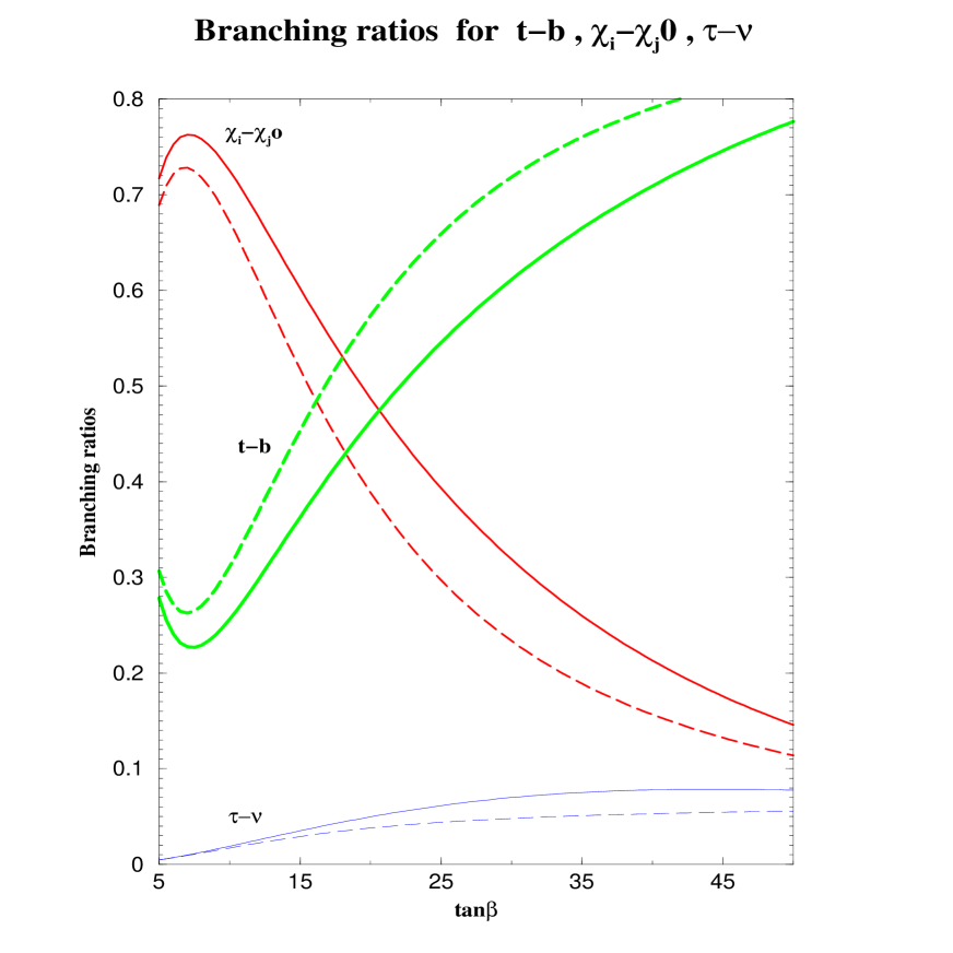
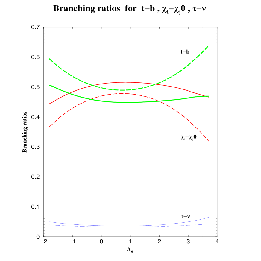
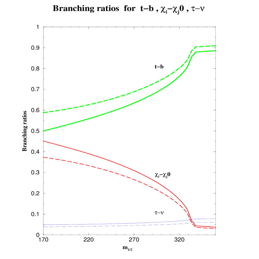
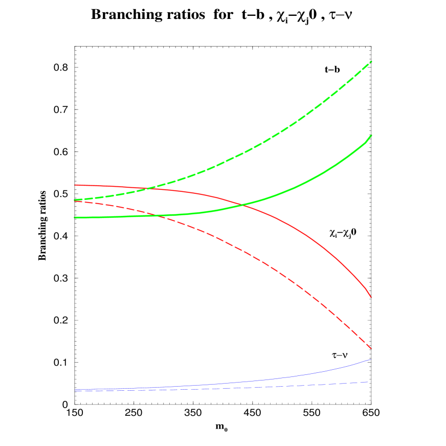
Figure 5: Plot of branching ratios for the decay of $H^{\pm}$ as a function of $\tan\beta$ in (a), as a function of $A_{0}$ in (b), as a function of $m_{\frac{1}{2}}$ in (c) and as a function of $m_{0}$ in (d). The parameters are $m_{A}=800$, $m_{0}=400$, $m_{\frac{1}{2}}=140$, $A_{0}$=3, $\tan\beta=20$, $\xi_{1}=0$, $\xi_{2}=0$, $\xi_{3}=0$, $\theta_{\mu}=0$, $\alpha_{A_{0}}=0$ except that the running parameter is to be deleted from the set for a given subgraph. The long dashed lines are the branching ratios at the tree level while the solid lines include the loop correction. The curves labelled $\chi_{i}^{-}\chi_{j}^{0}$ here and in Fig.(6) stand for sum of branching ratios into all allowed $\chi_{i}^{-}\chi_{j}^{0}$ modes. All masses are in unit of GeV and all angles in unit of radian.

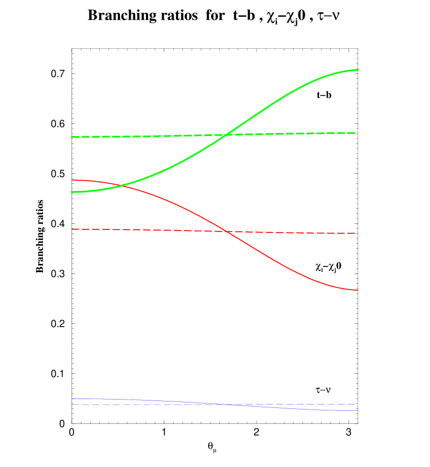
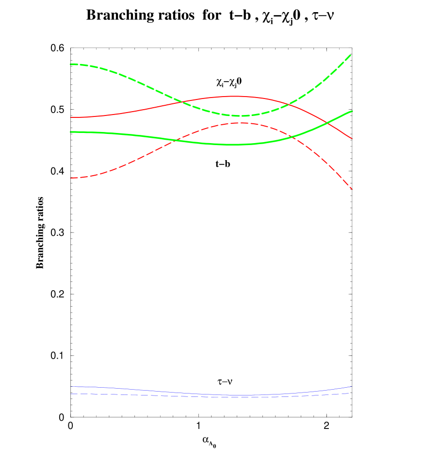
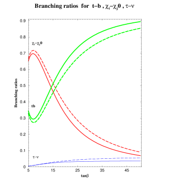
Figure 6: Plot of branching ratios for the decay of $H^{\pm}$ as a function of $\theta_{\mu}$ in (a) and as a function of $\alpha_{A_{0}}$ in (b). The parameters are $m_{A}=800$, $m_{0}=400$, $m_{\frac{1}{2}}=140$, $A_{0}$=3, $\tan\beta=20$, $\xi_{1}=0$, $\xi_{2}=0$, $\xi_{3}=0$, $\theta_{\mu}=0$, $\alpha_{A_{0}}=0$ except that the running parameter is to be deleted from the set for a given subgraph. The analysis of (c) corresponds to the input of Table 1 except that $\tan\beta$ is a running parameter. The long dashed lines are the branching ratios at the tree level while the solid lines include the loop correction. All masses are in unit of GeV and all angles in unit of radian.

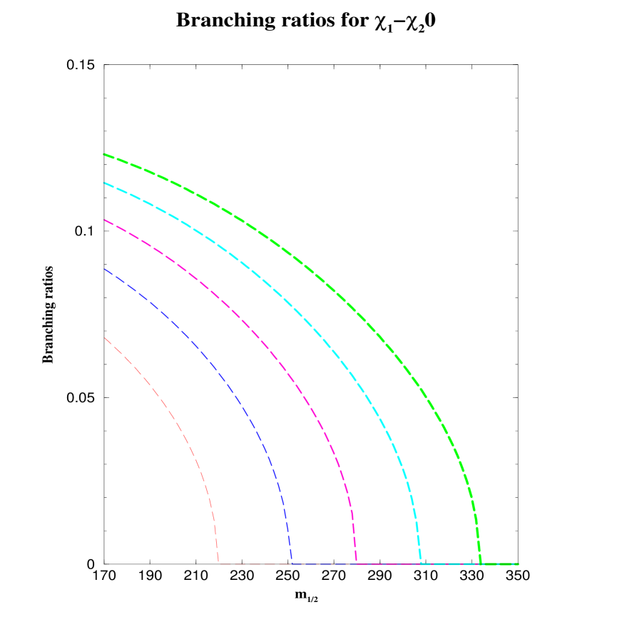
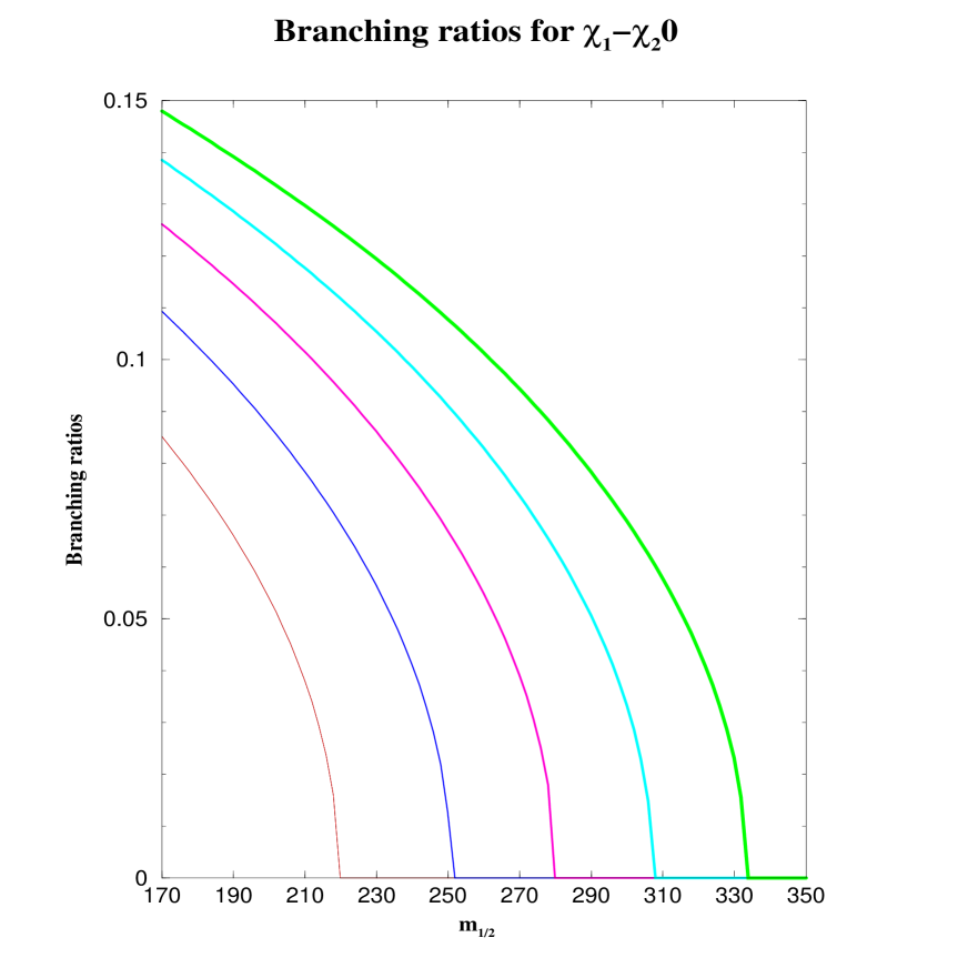
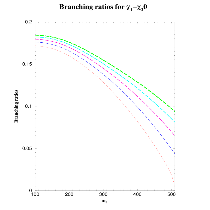
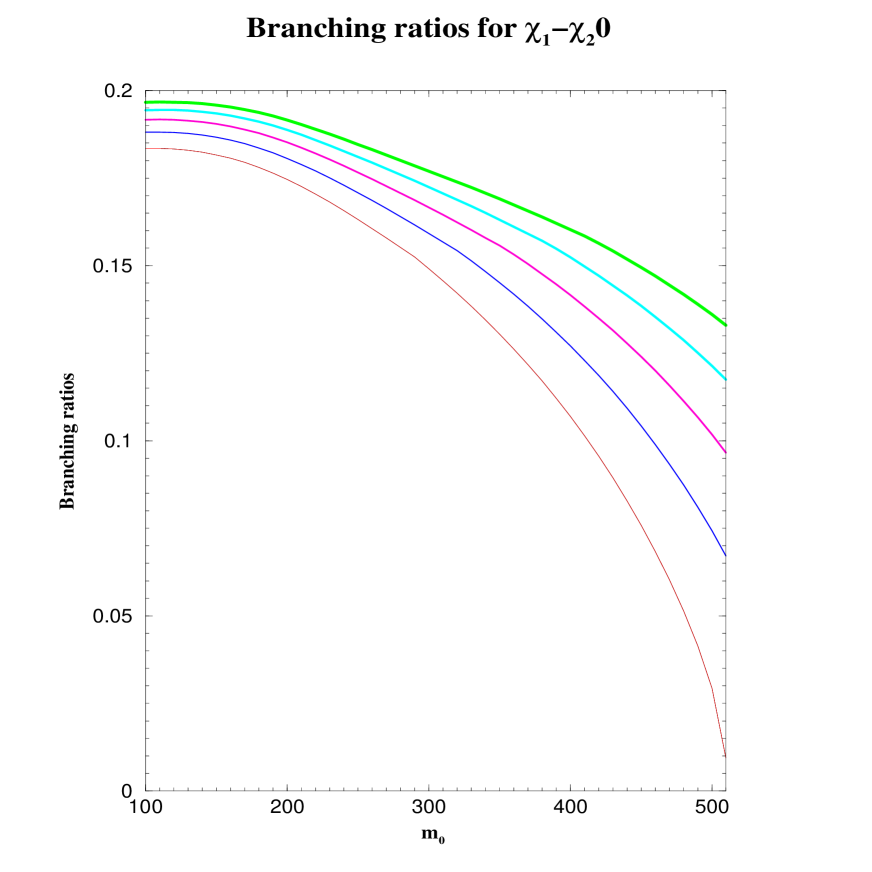
Figure 7: Plots of the branching ratio $\chi_{1}^{\pm}\chi_{2}^{0}$ for the decay of $H^{\pm}$ as a function of $m_{\frac{1}{2}}$ ( (a)-(b)), and as a function of $m_{0}$ ((c)-(d)). The common inputs are $\tan\beta=20$, $\xi_{1}=0$, $\xi_{2}=0$, $\xi_{3}=0$ , $A_{0}=3$, $\alpha_{A_{0}}=0$, and $\theta_{\mu}=0$ and $m_{A}$ ranges from $600-800$ in increments of $50$ in ascending order of curves. (a) -(b) have the additional input $m_{0}=400$ while (c)-(d) have the additional input $m_{\frac{1}{2}}=140$. (a) and (c) are for branching ratios at the tree level while (b) and (d) include the loop correction. All masses are in unit of GeV and angles in unit of radian.

References

[1]
For a recent review, see,
M. Carena and H. E. Haber,
Prog. Part. Nucl. Phys. 50, 63 (2003)
[arXiv:hep-ph/0208209].
[2] L.J. Hall, R. Rattazzi and U. Sarid, Phys. Rev D50,
7048 (1994); R. Hempfling, Phys. Rev D49, 6168 (1994); M. Carena,
M. Olechowski, S. Pokorski and C. Wagner, Nucl. Phys. B426, 269 (1994);
D. Pierce, J. Bagger, K. Matchev and R. Zhang, Nucl. Phys. B491,
3 (1997).
[3]
M. Carena, D. Garcia, U. Nierste and C. E. M. Wagner,
Nucl. Phys. B 577, 88 (2000)
[arXiv:hep-ph/9912516].
[4]
E. Christova, H. Eberl, W. Majerotto and S. Kraml,
JHEP 0212, 021 (2002)
[arXiv:hep-ph/0211063];
E. Christova, H. Eberl, W. Majerotto and S. Kraml,
Nucl. Phys. B 639, 263 (2002)
[Erratum-ibid. B 647, 359 (2002)]
[arXiv:hep-ph/0205227].
[5]
T. Ibrahim and P. Nath,
Phys. Rev. D 67, 095003 (2003)
[Erratum-ibid. D 68, 019901 (2003)]
[arXiv:hep-ph/0301110].
[6]
T. Ibrahim and P. Nath,
Phys. Rev. D 68, 015008 (2003)
[arXiv:hep-ph/0305201].
[7]
T. Ibrahim and P. Nath,
Phys. Rev. D 69, 075001 (2004)
[arXiv:hep-ph/0311242].
[8]
A.H. Chamseddine, R. Arnowitt and P. Nath, Phys. Rev. Lett. 49, 970 (1982); R. Barbieri, S. Ferrara and C.A. Savoy, Phys. Lett. B 119, 343 (1982); L. Hall, J. Lykken, and S. Weinberg,
Phys. Rev. D 27, 2359 (1983): P. Nath, R. Arnowitt and A.H. Chamseddine,
Nucl. Phys. B 227, 121 (1983).
For a recent review see, P. Nath,
“Twenty years of SUGRA,”
arXiv:hep-ph/0307123..
[9]
E. Commins, et. al., Phys. Rev. A50, 2960(1994).
[10]
P.G. Harris et.al., Phys. Rev. Lett. 82, 904(1999).
[11]
S. K. Lamoreaux, J. P. Jacobs, B. R. Heckel, F. J. Raab and E. N. Fortson,
Phys. Rev. Lett. 57, 3125 (1986).
[12]
P. Nath, Phys. Rev. Lett.66, 2565(1991);
Y. Kizukuri and N. Oshimo, Phys.Rev.D46,3025(1992).
[13]
T. Ibrahim and P. Nath, Phys. Lett. B 418, 98 (1998);
Phys. Rev. D57, 478(1998); Phys. Rev. D58, 111301(1998);
T. Falk and K Olive, Phys. Lett. B 439, 71(1998);
M. Brhlik, G.J. Good, and G.L. Kane, Phys. Rev. D59, 115004
(1999); A. Bartl, T. Gajdosik, W. Porod, P. Stockinger, and
H. Stremnitzer, Phys. Rev. 60, 073003(1999);
S. Pokorski, J. Rosiek and C.A. Savoy,
Nucl.Phys. B570, 81(2000);
E. Accomando, R. Arnowitt and B. Dutta,
Phys. Rev. D 61, 115003 (2000);
U. Chattopadhyay, T. Ibrahim, D.P. Roy, Phys.Rev.D64:013004,2001;
C. S. Huang and W. Liao,
Phys. Rev. D 61, 116002 (2000);
ibid, Phys. Rev. D 62, 016008 (2000);
A.Bartl, T. Gajdosik, E.Lunghi, A. Masiero, W. Porod,
H. Stremnitzer and O. Vives, hep-ph/0103324.
M. Brhlik, L. Everett, G. Kane and J. Lykken, Phys. Rev.
Lett. 83, 2124, 1999; Phys. Rev. D62, 035005(2000);
E. Accomando, R. Arnowitt and B. Datta,
Phys. Rev. D61, 075010(2000);
T. Ibrahim and P. Nath, Phys. Rev. D61, 093004(2000).
[14]
T. Falk, K.A. Olive, M. Prospelov, and R. Roiban, Nucl. Phys.
B560, 3(1999); V. D. Barger, T. Falk, T. Han, J. Jiang, T. Li
and T. Plehn,
Phys. Rev. D 64, 056007 (2001);
S.Abel, S. Khalil, O.Lebedev, Phys. Rev. Lett. 86, 5850(2001);
T. Ibrahim and P. Nath,
Phys. Rev. D 67, 016005 (2003)
arXiv:hep-ph/0208142.
[15]
D. Chang, W-Y.Keung,and A. Pilaftsis, Phys. Rev. Lett. 82,
900(1999).
[16]
A. Pilaftsis, Phys. Rev. D58, 096010; Phys. Lett.B435,
88(1998);
A. Pilaftsis and C.E.M. Wagner, Nucl. Phys. B553, 3(1999);
D.A. Demir, Phys. Rev. D60, 055006(1999);
S. Y. Choi, M. Drees and J. S. Lee,
Phys. Lett. B 481, 57 (2000);
T. Ibrahim and P. Nath,
Phys.Rev.D63:035009,2001; hep-ph/0008237;
T. Ibrahim,
Phys. Rev. D 64, 035009 (2001);
T. Ibrahim and P. Nath,
Phys. Rev. D 66, 015005 (2002);
S. W. Ham, S. K. Oh, E. J. Yoo, C. M. Kim and D. Son,
arXiv:hep-ph/0205244;
M. Boz,
Mod. Phys. Lett. A 17, 215 (2002).
;
M. Carena, J. R. Ellis, A. Pilaftsis and C. E. Wagner,
Nucl. Phys. B 625, 345 (2002)
[arXiv:hep-ph/0111245].
:
J. Ellis, J. S. Lee and A. Pilaftsis,
arXiv:hep-ph/0404167.
[17]
U. Chattopadhyay, T. Ibrahim and P. Nath,
Phys. Rev. D60,063505(1999);
T. Falk, A. Ferstl and K. Olive, Astropart. Phys. 13, 301(2000);
S. Khalil, Phys. Lett. B484, 98(2000);
S. Khalil and Q. Shafi, Nucl.Phys. B564, 19(1999);
K. Freese and P. Gondolo, hep-ph/9908390;
S.Y. Choi, hep-ph/9908397;
M. E. Gomez, T. Ibrahim, P. Nath and S. Skadhauge,
arXiv:hep-ph/040402;
T. Nihei and M. Sasagawa,
arXiv:hep-ph/0404100.
[18]
For a more complete set of references see,
T. Ibrahim and P. Nath,
“Phases and CP violation in SUSY,”
arXiv:hep-ph/0210251 published in
P. Nath and P. M. . Zerwas,
“Supersymmetry and unification of fundamental interactions.
Proceedings, 10th International Conference, SUSY’02, Hamburg, Germany, June 17-23,
2002,” DESY-PROC-2002-02
[19]
J. A. Grifols and A. Mendez,
Phys. Rev. D 22, 1725 (1980).
[20]
R. Arnowitt and P. Nath,
Phys. Rev. Lett. 69, 725 (1992).
[21]
T. Ibrahim and P. Nath,
Phys. Rev. D 58, 111301 (1998)
[arXiv:hep-ph/9807501].
[22]
J. F. Gunion and H. E. Haber,
Nucl. Phys. B 307, 445 (1988)
[Erratum-ibid. B 402, 569 (1993)].
[23]
D. A. Dicus, S. Nandi and X. Tata,
Phys. Lett. B 129, 451 (1983);
A. H. Chamseddine, P. Nath and R. Arnowitt,
Phys. Lett. B 129, 445 (1983);
H. Baer, K. Hagiwara and X. Tata,
Phys. Rev. D 35, 1598 (1987).
[24]
P. Nath and R. Arnowitt,
Mod. Phys. Lett. A 2, 331 (1987).
[25]
For a review and a more complete set of references, see
S. Abel et al. [SUGRA Working Group Collaboration],
arXiv:hep-ph/0003154. For a more recent update see,
H. Baer, T. Krupovnickas and X. Tata,
JHEP 0307, 020 (2003)
[arXiv:hep-ph/0305325].