GLUEBALLS, HYBRIDS, PENTAQUARKS:
Introduction to Hadron Spectroscopy
and Review of Selected Topics

Hadron spectroscopy has received revitalised interest due to the discovery of states with unexpected properties. The BABAR collaboration found a $\rm D_{sJ}(2317)$ (likely scalar) meson, accompanied by a second state, the $\rm D_{sJ}(2463)$ with preferred spin $J=1$, discovered at CLEO. Both are found at an unexpectedly low mass and are narrow. A further narrow resonance, discovered at BELLE in its decay into $\pi\pi$J/$\psi$, might be a $\rm DD^{*}$ molecule or a $c\bar{c}$ meson in which the color field, concentrated in a flux tube, is excited. A $q\bar{q}$ state with excited gluon field is called hybrid, such excitations are expected from QCD. The mass of the state at the $\rm DD^{*}$ threshold underlines the importance of meson–meson interactions or four–quark dynamics at the opening of new thresholds. BES reports a signal in radiative J/$\psi$ decays into a proton and an antiproton which has the properties as predicted for $N\bar{N}$ quasi-nuclear bound states. And last not least the $\Theta^{+}(1540)$, seen in several experiments, shows that the ’naive’ quark model needs to be extended. There is also considerable progress in understanding the dynamics of quarks in more conventional situations even though the view presented here is not uncontested. In meson and in baryon spectroscopy, evidence is emerging that one–gluon–exchange does not provide the appropiate means to understand low–energy QCD; instanton–induced interactions yield much more insight. In particular the rich spectrum of baryon resonances is very well suited to test dynamical quark models using constituent quarks, a confinement potential plus some residual interactions. The baryon spectrum favors definitely instanton–induced interactions over long–range one–gluon exchange. A still controversial issue is the question if glueballs and hybrids exist. There is the possibility that two $q\bar{q}$ scalar states and a glueball form three observed resonances by mixing. However, there is also rather conclusive evidence against this interpretation. Mesons with exotic quantum numbers have been reported but there is no reason why they should be hybrids: a four–quark interpretation is enforced for the $\pi_{1}(1400)$ and not ruled out in the other cases. This report is based on a lecture series which had the intent in the other cases. This report is based on a lecture series which had the intent to indroduce young scientists into hadron spectroscopy. The attempt is made to transmit basic ideas standing behind some models, without any formulae. Of course, these models require (and deserve) a much deeper study. However, it may be useful to explain in a simple language some of the ideas behind the formalisms. Often, a personal view is presented which is not shared by many experts working in the field. In the last section, the attempt is made to combine the findings into a picture of hadronic interactions and to show some of the consequences the picture entails and to suggest further experimental and theoretical work. This report is based on a lecture series which had the intent and so in the other cases. This file contains the abstract only. The full text with 27 Tables and 81 figures including a tar file is available at www.uni-bonn.de/ek/ hugs_proc.tar   

1 Getting started

1.1 Historical remarks

Nuclear interactions

In the beginning of the 1930’ties, three particles were known from which all matter is built: protons and neutrons form the nuclei and their charges are neutralized by very light electrons. The binding forces between electrons and nuclei were reasonably well understood as electromagnetic interaction but nobody knew why protons and neutrons stick together forming nuclei. Protons and neutrons have similar masses; Heisenberg suggested they be consider as one particle called nucleon. He proposed a new quantum number, isospin $I$, with $I=1/2,I_{3}=1/2$ for protons and $I=1/2,I_{3}=-1/2$ for neutrons. Pauli had suggested that a massless weakly interacting neutrino ($\nu$) should exist, but it was considered to be undetectable.

In 1935 Hideki Yukawa published an article $\!{}^{{\bf?}}$ in which he proposed a field theory of nuclear forces to explain their short range and predicted the existence of a meson, called $\pi$-meson or pion. While the Coulomb potential is given by

$$V_{QED}=\frac{e}{4\pi\epsilon_{0}r}$$ (1)

and originates from the exchange of photons with zero mass, Yukawa proposed that strong interactions may be described by the exchange of a particle having a mass of about 100 MeV leading to a potential with a range 1/$m_{\pi}$:

$$V_{strong}=\frac{g}{4\pi r}\cdot e^{-m_{\pi}r}.$$ (2)

The pion was discovered by C. Powell in 1947 $\!{}^{{\bf?}}$, and two years later Yukawa received the Nobel prize. We now know that there are 3 pions, $\pi^{+}$, $\pi^{0}$, and $\pi^{-}$. This is an isospin triplet with $I=1$ and the third component being $I_{3}=1,0$, or $-1$.

Resonances in strong interactions

In 1952 E. Fermi and collaborators measured the cross section for $\pi^{+}p\to\pi^{+}p$ and found it steeply rising $\!{}^{{\bf?}}$. Modern data (extracted from $\!{}^{{\bf?}}$) on $\pi N\to\pi N$ scattering are shown in figure 1. Cross sections are given for elastic and charge exchange scattering, with maximum cross sections

$\sigma_{tot,\pi^{+}p}=210$ mb	$\sigma_{tot,\pi^{-}p}=70$ mb
$\sigma_{el,\pi^{+}p}=210$ mb	$\sigma_{el,\pi^{-}p}=23$ mb.

The largest cross section occurs at an invariant mass of 1230 MeV. It is a resonance, called $\Delta(1232)$. It can be observed in four different charge states $\Delta^{++}(1232)$, $\Delta^{+}(1232)$, $\Delta^{0}(1232)$, $\Delta^{-}(1232)$. Like in the case of the nucleon these states are put into an isospin multiplet with $I=3/2$, and $I_{3}=3/2,I=1/2,I=-1/2$ and $I=-3/2$, respectively.

The $\Delta(1232)$ has a width of 150 MeV and thus a lifetime $\tau=\hbar/\Gamma\sim 0.45\ 10^{-23}$ s. This is really a short time; within $\tau$ a particle travels about 1 fm at the speed of light.

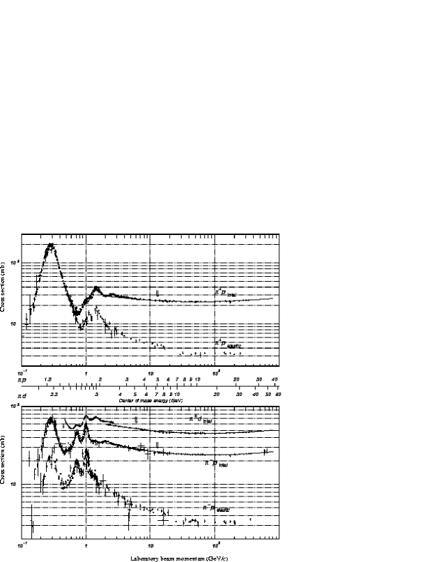
Figure 1: Cross sections for $\pi N$ scattering (from $\!{}^{{\bf?}}$)

.

Clebsch Gordan coefficients

The peak cross sections for $\Delta(1232)$ production in $\pi^{+}$p, $\pi^{-}$p elastic scattering and for $\pi^{-}$p charge exchange differ substantially. Moreover, there are further peaks, some of which show up only in $\pi^{-}$p scattering and not in $\pi^{+}$p. Here we can see the utility of the isospin concept. Pions have isospin 1, nucleons isospin 1/2. In strong interactions isospin is conserved: we can form two scattering amplitudes, one with isospin 3/2 (leading to the $\Delta(1232)$ and to $\Delta^{*}$ resonances) and one with isospin 1/2 which contains resonance excitations of the nucleon. $\pi^{+}$p is always isospin 3/2 (since $I_{3}=3/2$); $\pi^{-}$p can either have $I=1/2$ or $I=3/2$. The ratio is given by Clebsch–Gordan coefficients, the same as used to add angular momenta.

To understand the height of the various cross sections, these are compared to squared Clebsch–Gordan coefficients. It is a very useful exercise to look up these coefficients in a table and to compare the numbers with those listed explicitly below. The cross sections for $\Delta(1232)$ production scale as predicted from (squared) Clebsch–Gordan coefficients !

$\sigma_{tot,\pi^{+}p}$	=	$\sigma_{\pi^{+}p\to\pi^{+}p}$	=	210 mb	$\propto 1\times 1$
$\rm CG_{(I=1/2,I_{3}=1/2)+(I=1,I_{3}=1)\to(I=3/2,I_{3}=3/2)}\times CG_{(I=3/2,I_{3}=3/2)\to(I=1/2,I_{3}=1/2)+(I=1,I_{3}=1)}$
$\sigma_{el,\pi^{+}p}$	=	$\sigma_{\pi^{+}p\to\pi^{+}p}$	=	210 mb	$\propto 1\times 1$
$\rm CG_{(I=1/2,I_{3}=1/2)+(I=1,I_{3}=1)\to(I=3/2,I_{3}=3/2)}\times CG_{(I=3/2,I_{3}=3/2)\to(I=1/2,I_{3}=1/2)+(I=1,I_{3}=1)}$
$\sigma_{tot,\pi^{-}p}$	=	$\sigma_{\pi^{-}p\to\pi^{-}p}+\sigma_{\pi^{-}p\to\pi^{0}n}$	=	70 mb	$\propto 1/3\times 2/3+1/3\times 1/3$
$\rm CG_{(I=1/2,I_{3}=1/2)+(I=1,I_{3}=-1)\to(I=3/2,I_{3}=-1/2)}+CG_{(I=1/2,I_{3}=-1/2)+(I=1,I_{3}=0)+(I=3/2,I_{3}=-1/2)}$
$\sigma_{el,\pi^{-}p}$	=	$\sigma_{\pi^{-}p\to\pi^{-}p}$	=	23 mb	$\propto 1/3\times 1/3$
$\rm CG_{(I=1/2,I_{3}=1/2)+(I=1,I_{3}=-1)\to(I=3/2,I_{3}=-1/2)}\times CG_{(I=3/2,I_{3}=-1/2)\to(I=1/2,I_{3}=1/2)+(I=1,I_{3}=-1)}$

The particle zoo

In the same year 1949, Rochester and Butler $\!{}^{{\bf?}}$ found reactions of the type ${\rm\pi^{-}p\mbox{$\rightarrow$}\ \Lambda K_{s}^{0}}$ where both particles had long lifetimes, on the order of $10^{-10}\,s$. This seems to be a short time but when we consider the $\rm K_{s}^{0}$ as a composite particle like positronium (the $\rm e^{+}e^{-}$ analogue of hydrogen atoms) consisting of a quark and an antiquark rotating with the velocity of light and a radius of 0.5 fm, then the $\rm K_{s}^{0}$ lives for $\sim 10^{13}$ revolutions. A fantastically long life time ! The earth has only encircled the sun for $5\cdot 10^{9}$ revolutions. The surprise was that these particles are produced via strong interactions and in pairs (in this case a $\rm K_{s}^{0}$ and a $\Lambda$). This phenomenon was called associated production by Pais in 1952 $\!{}^{{\bf?}}$. Both particles decay by weak interaction. To explain this strange behavior, production by strong interactions and decay via weak interactions, a new additive quantum number was introduced called strangeness $S$. Strangeness is produced as $S$ and anti-$S$ (or $\bar{S}$) pairs and conserved in strong interactions. The $\Lambda$, e.g., carries strangeness $S=-1$ and does not decay via strong interactions. Instead, as all strange particles, it decays via weak interactions, $\rm\Lambda\to N\pi$, with a long life time.

The first idea was to consider the proton, neutron, and the $\Lambda$ as building blocks in nature but more and more strongly interacting particles were discovered and the notion ’the particle zoo’ was created. In particular there are 3 pions having a mass of 135 MeV, the $\pi^{+},\pi^{-}$ and the $\pi^{0}$; the $\eta(547)$ and $\eta^{\prime}(958)$; and four Kaons K⁺, K^-, K${}^{0}_{s}$, K${}^{0}_{l}$ having a mass close to 500 MeV. All these particles have spin 0. The three $\rho^{+-0}(770)$, the $\omega(782)$, the $\Phi(1020)$ and four $\rm K^{*}(892)$ have spin 1 and there are particles with spin 2, i.e. the $\rm a_{2}(1320)$ and $\rm f_{2}(1270)$, among others. These particles have, like photons, integer spins; they are bosons obeying Bose symmetry: the wave function of, let us say $n_{\pi^{0}}$ neutral pions, must be symmetric with respect to the exchange of any pair of $\pi^{0}$’s. All these particles can be created or destroyed as the number of bosons is not a conserved quantum number.

Protons, neutrons and $\Lambda$’s are different: they have spin 1/2 and obey Fermi statistics. A nuclear wave function must be antisymmetric when two protons are exchanged. These particles are called baryons. The number of baryons is a conserved quantity. More baryons were discovered, $\Sigma^{+}$, $\Sigma^{0}$, $\Sigma^{-}$ with three charge states, pair $\Xi^{0}$, $\Xi^{-}$, the $\Delta(1232)$ and many more.

Of course not all of these particles can be ’fundamental’. In 1964, Gell-Mann suggested the quark model $\!{}^{{\bf?}}$. He postulated the existence of three quarks called up $(u)$, down $(d)$, and strange $(s)$. All baryons can then be classified as bound systems of three quarks, and mesons as bound states of one quark and one antiquark. With the quarks $u,d,s$ we expect families (with identical spin and parities) of 9 mesons. This is indeed the case. Baryons consist of 3 quarks, $qqq$. We might expect families of 27 baryons but this is wrong; the Pauli principle reduces the number of states.

Color

In the quark model, the $\Delta^{++}(1232)$ consists of three $u$ quarks with parallel spin, all in an $S$–wave. Quarks are Fermions and the Pauli principle requires the wave function to be antisymmetric with respect to the exchange of two identical quarks. Hence the three quarks cannot be identical. A possible solution is the introduction of a further quark property, the so–called color. There are three colors, red, green, and blue. A baryon then can be written as the determinant of three lines $q_{1}$, $q_{2}$, $q_{3}$, and three rows, flavor, spin, color. The determinant has the desired antisymmetry. When color was introduced $\!{}^{{\bf?}}$ it was to ensure antisymmetry of baryon wave functions. It was only with the advent of quantum chromodynamics that color became a source of gluon fields and resumed a decisive dynamical role. Colored quarks and gluons interact via exchange of gluons in the same way as charges interact via exchange of photons.

Units

We use $\hbar=c=1$ in these lecture notes. The fine structure constant is defined as

$$\alpha=\frac{e^{2}}{4\pi\epsilon_{0}\hbar c}=1/137.036.$$ (3)

The factor $4\pi\epsilon_{0}\hbar c$ depends on the units chosen; but one does not need to remember units. If you take a formula from a textbook, look up the Coulomb potential and replace it with $eV_{Coulomb}=\alpha/r$. If there is a factor $4\pi\epsilon_{0}$ or $\epsilon_{0}$ in a formula, replace it by 1 whenever it occurs. (But remember wether $4\pi\epsilon_{0}$ or $\epsilon_{0}$ is equal to 1 !) If there is electron charge $e$ the interaction will be $e^{2}$, which is $\alpha$.

A second important number to remember is

$$\hbar c=197.327(\sim 200)\ {\mathrm{M}eV\,fm}.$$ (4)

If your final number does not havethe units you want, multiply with $\hbar c$ and with $c$ until you get the right units. It sounds like a miracle, but this technique works.

1.2 Mesons and their quantum numbers

Quarks have spin $S=1/2$ and baryon number $B=1/3$, antiquarks $S=1/2$ and $B=-1/3$. Quarks and antiquarks couple to $B=0$ and spin $S=1$ or $S=0$. Conventional mesons can be described as $q\bar{q}$ systems and thus have the following properties.

The parity due to angular momentum is $P=(-1)^{L}$. Quarks have intrinsic parity which we define to be $P=1$; antiquarks have opposite parity (this follows from the Dirac equation). The parity of a $q\bar{q}$ meson is hence given by

$$P=(-1)^{L+1}.$$ (5)

Neutral mesons with no strangeness are eigenstates of the charge conjugation operator, sometimes called $C$–parity,

$$C=(-1)^{L+S}$$ (6)

which is only defined for neutral mesons. A proton and neutron form a isospin doublet with $I=1/2$, $I_{3}=\pm 1/2$ for (p,n). The three pions have isospin $I=1$. From these quantum numbers we can define the $G$-parity

$$G=(-1)^{L+1+I}$$ (7)

which is approximately conserved in strong interactions. However, chiral symmetry is not an exact symmetry, and $G$–parity can be violated like in $\eta\to 3\pi$ or in $\omega\to 2\pi$ decays.

We can use these quantum numbers to characterize a meson by its $J^{PC}$ values. These are measured quantities. We may also borrow the spectroscopic notation ${}^{2s+1}L_{J}$ from atomic physics. Here, $s$ is the total spin of the two quarks, $L$ their relative orbital angular momentum and $J$ the total angular momentum.

The mesons with lowest mass have $L=0$ and the two quark spins have opposite directions: $\vec{s}_{1}+\vec{s}_{2}=0$. This leads to quantum numbers $J^{PC}=0^{-+}$. These mesons form the nonet of pseudoscalar mesons

with $\pi^{0}=\frac{1}{\sqrt{2}}\left|u\bar{u}-d\bar{d}\right>$, $\eta_{8}=\frac{1}{\sqrt{6}}\left|u\bar{u}+d\bar{d}-2s\bar{s}\right>$, and $\eta_{1}=\frac{1}{\sqrt{3}}\left|u\bar{u}+d\bar{d}+s\bar{s}\right>$.

Mixing angles

The two states $\eta_{8}$ and $\eta_{1}$ have identical quantum numbers, hence they can mix; the mixing angle is denoted by $\Theta_{ps}$:

$\eta$	=	$\cos\Theta_{ps}\,\eta_{8}$	-	$\sin\Theta_{ps}\,\eta_{1}$
$\eta^{\prime}$	=	$\sin\Theta_{ps}\,\eta_{8}$	+	$\cos\Theta_{ps}\,\eta_{1}$

Apart from these well established $\bar{q}q$ mesons, other kinds of mesons could also exist: glueballs, mesons with no (constituent) $\bar{q}q$ content, hybrids in which the binding fields between $\bar{q}$ and $q$ are excited, or multiquark states like $\bar{q}\bar{q}qq$ or meson–meson molecular–type states. As we will see, these are predicted by theory. We may then cautiously extend the mixing scheme to include a possible glueball content

$\eta$	=	${X_{\eta}}\cdot\frac{1}{\sqrt{2}}\left|\,u\bar{u}+d\bar{d}\,\right>$	+	${Y_{\eta}}\cdot\left|\,s\bar{s}\,\right>$	+	${Z_{\eta}}\cdot\left|\,{\rm glue}\,\right>$
$\eta^{\prime}$	=	${X_{\eta^{\prime}}}\cdot\frac{1}{\sqrt{2}}\left|\,u\bar{u}+d\bar{d}\,\right>$	+	${Y_{\eta^{\prime}}}\cdot\left|\,s\bar{s}\,\right>$	+	${Z_{\eta^{\prime}}}\cdot\left|\,{\rm glue}\,\right>$
		light quark		strange quark		inert

Experimentally it turns out that ${Z_{\eta}=Z_{\eta^{\prime}}\sim 0}$. The pseudoscalar glueball, if it exists, does not mix strongly with the ground–state pseudoscalar mesons $\!{}^{{\bf?}}$.

Mixing angles, examples

We now write down the wave functions for a few special mixing angles. We define $n\bar{n}=1/\sqrt{2}(u\bar{u}+d\bar{d})$.

$\Theta_{PS}=0^{\circ}$	$\left|\eta\right\rangle=\sqrt{\frac{1}{3}}\,\left|n\bar{n}-\sqrt{2}s\bar{s}\right\rangle$	$\left|\eta^{\prime}\right\rangle=\sqrt{\frac{2}{3}}\,\left|n\bar{n}+\frac{1}{\sqrt{2}}s\bar{s}\right\rangle$
$\Theta_{PS}=-11.1^{\circ}$	$\left|\eta\right\rangle=\frac{1}{\sqrt{2}}\,\left|n\bar{n}-s\bar{s}\right\rangle$	$\left|\eta^{\prime}\right\rangle=\frac{1}{\sqrt{2}}\,\left|n\bar{n}+s\bar{s}\right\rangle$
$\Theta_{PS}=-19.3^{\circ}$	$\left|\eta\right\rangle=\sqrt{\frac{2}{3}}\,\left|n\bar{n}-\frac{1}{\sqrt{2}}s\bar{s}\right\rangle$	$\left|\eta^{\prime}\right\rangle=\sqrt{\frac{1}{3}}\,\left|n\bar{n}+\sqrt{2}s\bar{s}\right\rangle$
$\Theta_{PS}=\Theta_{ideal}=35.3^{\circ}$	$\left|\eta\right\rangle=\left|s\bar{s}\right\rangle$	$\left|\eta^{\prime}\right\rangle=\left|n\bar{n}\right\rangle$

For $\Theta_{PS}=0$ we retain the octet and singlet wave functions. $\Theta_{PS}=-11.1^{\circ}$ is used often in older literature; with this mixing angle, $\eta$ and $\eta^{\prime}$ have the same strangeness content. For $\Theta_{PS}=-19.3^{\circ}$, the wave function is similar to the octet/singlet wave functions, except for the sign. The $\bar{s}s$ component in the $\eta^{\prime}$ is now twice as strong as in the $\eta$. Finally $\Theta_{PS}=35.3^{\circ}$ gives a decoupling of the $\bar{s}s$ from $(u\bar{u}+d\bar{d})$. This is the ideal mixing angle. For most meson nonets the mixing angle is approximately ideal. Exceptions are the nonet of pseudoscalar and scalar mesons.

For $L=0$ and $\vec{s}_{1}+\vec{s}_{2}=\vec{S}$ and $S=1$ we get the nonet of vector mesons with $J^{PC}=1^{--}$. Additionally there can be orbital angular momentum between the quark and antiquark, and $\vec{L}$ and $\vec{S}$ can combine to $J=2$ thus forming the nonet of tensor mesons with $J^{PC}=2^{++}$.

The vector and tensor mixing angles, $\Theta_{V}$ and $\Theta_{T}$, are both close to $35.3^{\circ}$. Hence we have

$\omega$	=	$\frac{1}{\sqrt{2}}\left(u\bar{u}+d\bar{d}\right)$	$\Phi$	=	$s\bar{s}$
$f_{2}(1270)$	=	$\frac{1}{\sqrt{2}}\left(u\bar{u}+d\bar{d}\right)$	$f_{2}(1525)$	=	$s\bar{s}$

Quarks and antiquarks can have any orbital angular momentum. Combined with the spin, there is a large variety of mesons which can be formed. Not all of them are known experimentally. Their masses provide constraints for the forces which tie together quarks and antiquarks.

The Gell-Mann-Okubo mass formula

We now assume that mesons have a common mass $M_{0}$ plus the mass due to its two flavor-dependent quark masses $M_{q_{1}}$ and $M_{q_{2}}$. Then the masses can be written as

$$M_{\pi} = M_{0}+2M_{q}$$

$$M_{K} = M_{0}+M_{q}+M_{s}$$

$$M_{\eta} = M_{8}\cos^{2}\Theta+M_{1}\sin^{2}\Theta$$

$$M_{\eta^{\prime}} = M_{8}\sin^{2}\Theta+M_{1}\cos^{2}\Theta$$

$$M_{1}=M_{0}+4/3M_{q}+2/3M_{s}$$

$$M_{8}=M_{0}+2/3M_{q}+4/3M_{s}$$

From these equations we derive the linear mass formula:

$$\tan^{2}\Theta=\frac{3M_{\eta}+M_{\pi}-4M_{K}}{4M_{K}-3M_{\eta^{\prime}}-M_{\pi}}$$ (8)

The Gordon equation is quadratic in mass, hence we may also try the quadratic mass formula $\!{}^{{\bf?}}$:

$$\tan^{2}\Theta=\frac{3M^{2}_{\eta}+M_{\pi}^{2}-4M_{K}^{2}}{4M_{K}^{2}-3M^{2}_{\eta^{\prime}}-M_{\pi}^{2}}$$ (9)

A better justification for the quadratic mass formula is the fact that in first order of chiral symmetry breaking, squared meson masses are linearly related to quark masses.

Nonet members	$\Theta_{\rm linear}$	$\Theta_{\rm quad}$
$\pi,K,\eta^{\prime},\eta$	$-23^{\circ}$	$-10^{\circ}$
$\rho,K^{*},\Phi\ ,\omega$	$36^{\circ}$	$39^{\circ}$
$a_{2}(1320),K^{*}_{2}(1430),f_{2}(1525),f_{2}(1270)$	$26^{\circ}$	$29^{\circ}$

Naming scheme

In table 1 a summary of light mesons for intrinsic orbital angular momenta up to 4 is given.

Regge trajectories

The squared meson masses are linearly dependent on the total angular momentum J, meson resonances lie on Regge trajectories $\!{}^{{\bf?}}$. Figure 2 shows such a plot for light $\bar{n}n$ mesons with $J=L+1$. The mesons belong to nonets with an approximately ideal mixing angle; the masses of the $\bar{u}u\pm\bar{d}d$ mesons are degenerate. Their mean value is used. The dotted line represents a fit to the meson masses taken from the PDG $\!{}^{{\bf?}}$; the error in the fit is given by the PDG errors and a second systematic error of 30 MeV is added quadratically. The slope is determined to 1.142 GeV².

Table 1 contains only the ground states, but as in atomic physics there are also radial excitations, states with wave functions having nodes. The $\rho$ meson for example is the $1^{3}S_{1}\rho(770)$ ground state. It has a radial excitation denoted as $2^{3}S_{1}\rho(1440)$. The state $1^{3}D_{1}\rho(1700)$ has the same measurable quantum numbers $J^{PC}=1^{--}$. Generally we cannot determine the internal structure of a meson with

Table 1: Naming scheme for light mesons

		$J^{PC}$	${}^{2s+1}L_{J}$	I=1	I=0 $(n\bar{n})$	I=0 $(s\bar{s})$	I=1/2
L=0	S=0	$0^{-+}$	${}^{1}S_{0}$	$\pi$	$\eta$	$\eta^{\prime}$	$K$
	S=1	$1^{--}$	${}^{3}S_{1}$	$\rho$	$\omega$	$\Phi$	$K^{*}$
L=1	S=0	$1^{+-}$	${}^{1}P_{1}$	$b_{1}$	$h_{1}$	$h_{1}^{\prime}$	$K_{1}$
	S=1	$0^{++}$	${}^{3}P_{0}$	$a_{0}$	$f_{0}$	$f_{0}^{\prime}$	$K_{0}^{*}$
		$1^{++}$	${}^{3}P_{1}$	$a_{1}$	$f_{1}$	$f_{1}^{\prime}$	$K_{1}$
		$2^{++}$	${}^{3}P_{2}$	$a_{2}$	$f_{2}$	$f_{2}^{\prime}$	$K_{2}^{*}$
L=2	S=0	$2^{-+}$	${}^{1}D_{2}$	$\pi_{2}$	$\eta_{2}$	$\eta_{2}^{\prime}$	$K_{2}$
	S=1	$1^{--}$	${}^{3}D_{1}$	$\rho$	$\omega$	$\Phi$	$K_{1}^{*}$
		$2^{--}$	${}^{3}D_{2}$	$\rho_{2}$	$\omega_{2}$	$\Phi_{2}$	$K_{2}$
		$3^{--}$	${}^{3}D_{3}$	$\rho_{3}$	$\omega_{3}$	$\Phi_{3}$	$K_{3}^{*}$
L=3	S=0	$3^{+-}$	${}^{1}F_{3}$	$b_{3}$	$h$	$h^{\prime}_{3}$	$K_{3}$
	S=1	$2^{++}$	${}^{3}F_{2}$	$a_{2}$	$f_{2}$	$f_{2}^{\prime}$	$K_{2}^{*}$
		$3^{++}$	${}^{3}F_{3}$	$a_{3}$	$f_{3}$	$f_{3}^{\prime}$	$K_{3}$
		$4^{++}$	${}^{3}F_{4}$	$a_{4}$	$f_{4}$	$f_{4}^{\prime}$	$K_{4}^{*}$
L=4	S=0	$4^{-+}$	${}^{1}G_{2}$	$\pi_{4}$	$\eta_{4}$	$\eta_{4}^{\prime}$	$K_{4}$
	S=1	$3^{--}$	${}^{3}G_{1}$	$\rho_{3}$	$\omega_{3}$	$\Phi_{3}$	$K_{3}^{*}$
		$4^{--}$	${}^{3}G_{2}$	$\rho_{4}$	$\omega_{4}$	$\Phi_{4}$	$K_{4}$
		$5^{--}$	${}^{3}G_{3}$	$\rho_{5}$	$\omega_{5}$	$\Phi_{5}$	$K_{5}^{*}$

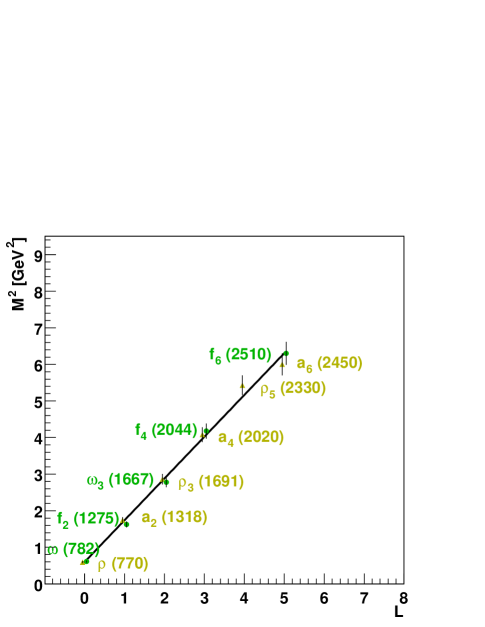
Figure 2: Regge trajectory for mesons with $J=L+1$.

given quantum numbers $J^{PC}$ and a given mass. A spectroscopic assignment requires models but a given state can be assigned to a spectroscopic state on the basis of its decays or due to its mass. Of course, mixing is possible between different internal configurations.

In figure 3 squared meson masses are plotted all having the same quantum numbers $J^{PC}$. The $\rho(770)$ as $1^{3}S_{1}$ is followed by the $2^{3}S_{1}$ and $3^{3}S_{1}$. A new sequence is started for the $1^{3}D_{1}$, $2^{3}D_{1}$, and $3^{D}S_{1}$. Likewise, $L=2$ and $L=4$ can couple to form two $J^{PC}=3^{--}$ series. Figure 3 is taken from $\!{}^{{\bf?}}$.

$\hskip 267.45572pt{}^{3}F_{4}\;q\bar{q}(L=3)$

$\hskip 267.45572pt{}^{3}F_{2}\;q\bar{q}(L=3)$

$\hskip 34.1433pt{}^{3}D_{1}\;q\bar{q}(L=2)\hskip 48.36967pt^{3}G_{3}\;q\bar{q}(L=4)\hskip 51.21495pt^{3}P_{2}\;q\bar{q}(L=1)$

$\hskip 34.1433pt{}^{3}S_{1}\;q\bar{q}(L=0)\hskip 51.21495pt^{3}D_{3}\;q\bar{q}(L=2)\hskip 51.21495pt^{3}P_{0}\;q\bar{q}(L=1)$

Figure 3: Mesons of identical $J^{PC}$ fall onto linear trajectories with a slope $(1.15-1.30)$ GeV² which is similar to the Regge slope found in figure 2. Note that many resonances shown here are not listed by the PDG. Hence some interpretation of the data is required. (The data are from $\!{}^{{\bf?}}$).

1.3 Charmonium and bottonium

Discovery of the J/$\psi$

A narrow resonance was discovered in 1974 in two reactions. At Brookhaven National Laboratory (BNL) in Long Island, New York, the process proton + Be $\to e^{+}e^{-}$ + anything was studied $\!{}^{{\bf?}}$; at the Stanford University, the new resonance was observed in the SPEAR storage ring in $e^{+}e^{-}$ annihilation to $\mu^{+}\mu^{-},e^{+}e^{-}$ and into hadrons $\!{}^{{\bf?}}$ This discovery initiated the “November revolution of particle physics”.

Electrons and positrons are rarely produced in hadronic reactions. Dalitz pairs (from $\pi^{0}\to\gamma e^{+}e^{-}$) have very low invariant masses; the probability to produce an $e^{+}e^{-}$ pair having a large invariant mass is very small. In the BNL experiment $e^{+}e^{-}$ pairs with large invariant masses were observed. The two particles were identified by Cerenkov radiation and time–of–flight, their momenta were measured in two spectrometers. In the $e^{+}e^{-}$ invariant mass distribution, $M^{2}=(\sum E_{i})^{2}-(\sum\vec{p}_{i})^{2}$, a new resonance showed up which was named $J$. This type of experiment is called a production experiment. In production experiments the width of a narrow peak is given by the resolution of the detector.

SPEAR was a $e^{+}e^{-}$ storage ring in which $e^{+}$ and $e^{-}$ pairs annihilated into virtual photons. These virtual photons couple to mesons (having the same quantum numbers as photons), to $J^{PC}=1^{--}$ vector mesons. The momenta of $e^{+}$ and $e^{-}$ are the same in magnitude but opposite in sign. Vector mesons are formed when the total energy W, often called $\sqrt{s}$, coincides with their mass. W is varied while scanning the resonance. The width of a narrow peak is given by the accuracy with which the beams can be tuned. This type of experiment is called a formation experiment.

Figure 4 shows (see http://bes.ihep.ac.cn/besI&II/physics/JPSI/index.html) a modern scan of the beam energy across a resonance which was named $\psi$. It is the same resonance as the $J$ particle, hence its name J/$\psi$. The width of the resonance is less than the spread of the beam energies, which is less than 1 MeV. Due to the production mode via an intermediate virtual photon, spin, parity and charge conjugation are $J^{PC}=1^{--}$ (as the $\rho$-meson). The J/$\psi$ is a vector meson.

Width of the J/$\psi$

The natural width of the J/$\psi$ is too narrow to be determined from figure 4 but it is related to the total cross section. The cross section can be written in the form

$$\sigma(E)=(4\pi)(\lambda^{2}/4\pi^{2})\frac{\Gamma^{2}/4}{\left[\left(E-E_{R}\right)+\Gamma^{2}/4\right)]}\frac{2J+1}{(2s_{1}+1)(2s_{2}+1)}$$ (10)

with $\lambda/2\pi=1/p=2/E$ being the de Broglie wave length of $e^{+}$ and $e^{-}$ in the

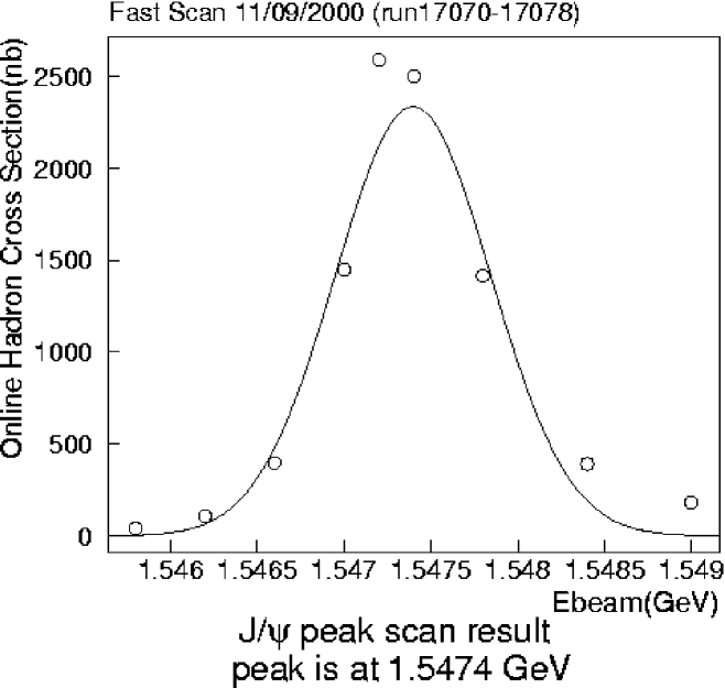
Figure 4: Scan of the beam energies in $e^{+}e^{-}$ scattering through the J/$\psi$ resonance region; (see http://bes.ihep.ac.cn/besI&II/physics/ JPSI/index.html).

center–of–mass system (cms), $E$ the cms energy, and $\Gamma$ the total width. The first term of the right–hand side of (10) is the usual Breit–Wigner function describing a resonant behavior. The second part sums over the spin components in the final state and averages over the spin components in the initial state. $s_{1}=s_{2}=1/2$ are electron and positron spin; $J=1$ is the J/$\psi$ total angular momentum.

In case of specific reactions, like $e^{+}e^{-}\to\psi\to e^{+}e^{-}$, we have to replace the total width in the numerator by

$$\Gamma^{2}\to\Gamma_{initial}\Gamma_{final}=\Gamma^{2}_{e^{+}e^{-}},$$ (11)

where $\Gamma_{e^{+}e^{-}}$ is the partial width for the decay into $e^{+}e^{-}$. Then:

$$\sigma(E_{e^{+}e^{-}\to\psi\to e^{+}e^{-}})=(3\pi)(\lambda^{2}/4\pi^{2})\frac{\Gamma^{2}_{e^{+}e^{-}}/4}{\left(E-E_{R}\right)+\Gamma^{2}/4}$$ (12)

The number of $e^{+}e^{-}$ pairs is proportional to

$$\int_{0}^{\infty}\sigma(E)dE=\frac{3\pi^{2}}{2}\frac{\lambda^{2}}{4\pi^{2}}\frac{\Gamma^{2}_{e^{+}e^{-}}}{\Gamma^{2}}\Gamma.$$ (13)

After substituting $\tan\theta=2(E-E_{R})/\Gamma$ the integration can be carried out and results in

$$\int_{0}^{\infty}\sigma(E_{e^{+}e^{-}\to e^{+}e^{-},\mu^{+}\mu^{-},\mathrm{hadrons}})dE=\frac{6\pi^{2}}{E_{R}^{2}\Gamma}\Gamma_{e^{+}e^{-}}\Gamma_{(e^{+}e^{-},\mu^{+}\mu^{-},\mathrm{hadrons})}.$$ (14)

The total width is given by the sum of the partial decay widths:

$$\Gamma=\Gamma_{e^{+}e^{-}}+\Gamma_{\mu^{+}\mu^{-}}+\Gamma_{hadrons}$$ (15)

Imposing $\Gamma_{e^{+}e^{-}}=\Gamma_{\mu^{+}\mu^{-}}$ yields 3 equations and thus 3 unknown widths.

The J/$\psi$ has a mass $(3096.87\pm 0.04)$ MeV and a width $87\pm 5$ keV. We may compare this to the $\rho$ mass, 770 MeV, and its width 150 MeV. Obviously the J/$\psi$ is extremely narrow. This can be understood by assuming that the J/$\psi$ is a bound state of a new kind of quarks called charmed quarks $c$, and that

J/$\psi=c\bar{c}$.

The Okubo–Zweig–Ishida (OZI) rule then explains why the J/$\psi$ is so narrow.

The OZI rule and flavor tagging

A low–lying $c\bar{c}$ bound state cannot decay into two $D$ mesons having open charm (see figure 5). The J/$\psi$ must annihilate completely and new particles have to be created out of the vacuum. Such processes are suppressed; the four-momentum of the $c\bar{c}$ bound state must convert into gluons carrying a large four-momentum, and we will see in section 3 that the coupling of quarks to gluons with large four-momenta is small. Hence the J/$\psi$ is narrow. This OZI rule can be exploited to tag the flavor of mesons produced in J/$\psi$ decays in cases where one of the two mesons has a known flavor content. If it is a $\bar{u}u+\bar{d}d$ meson, like the $\omega$, the recoiling meson couples with its $\bar{u}u+\bar{d}d$ component. If a $\Phi(1020)$ meson is produced, the recoiling meson couples with its $\bar{s}s$ component. Thus the flavor structure of mesons can be determined. This was done for the $\eta$ and $\eta^{\prime}$ mesons and led to the pseudoscalar mixing angle as discussed above $\!{}^{{\bf?},{\bf?}}$.

Figure 5: Decays of charmonium states into $\rm\bar{D}D$ are allowed only above the $\rm\bar{D}D$ threshold, the J$/\psi$ (and the $\eta_{c}$ and $\chi$ states) can decay only into light quarks. A $\omega$ or $\Phi(1020)$ signal determines the $\bar{u}u+\bar{d}d$ and $\bar{s}s$ component, respectively, of the recoiling meson. The thick lines represent charmed quarks.

The cross section for $e^{+}e^{-}$ annihilation into hadrons shown in figure 6 gives access to a variety of physics questions. At low energies the cross section is dominated by $\rho,\omega$ and $\Phi$ mesons. Then it falls off according to $(4\pi\alpha^{2}/3\,s)\cdot 3\cdot\sum Q^{2}_{i}$ where $Q_{i}$ are the quark charges and the sum extends over all quarks which can be created at the given energy. The factor $3$ accounts for the three different colors. There are two narrow $c\bar{c}$ states, the J/$\psi$ and the $\psi(2S)$, and three narrow $b\bar{b}$ states, the $\Upsilon,\Upsilon(2S)$, and $\Upsilon(3S)$. At 90 GeV the $Z^{0}$ resonance, the neutral weak interaction boson, is observed. The ratio $R$ of the cross section for $e^{+}e^{-}\to$ hadrons to that for $\mu^{+}\mu^{-}$ is given by $R=3\times\sum Q_{i}^{2}$ and increases above quark-antiquark thresholds. In figure 7 we see that $R$ increases from the value 2.2 below the J/$\psi$ to 3.7 above. For quarks with charges 2/3 we expect an increase of $3\times(2/3)^{2}=4/9\simeq 0.44$. To account for the observed increase we have to include $\tau^{+}\tau^{-}$ production, setting in at about the open $\bar{c}c$ threshold. The $\tau$ charge is $1$, so $R$ should increase by 1.44, apart from corrections due to gluon radiation.

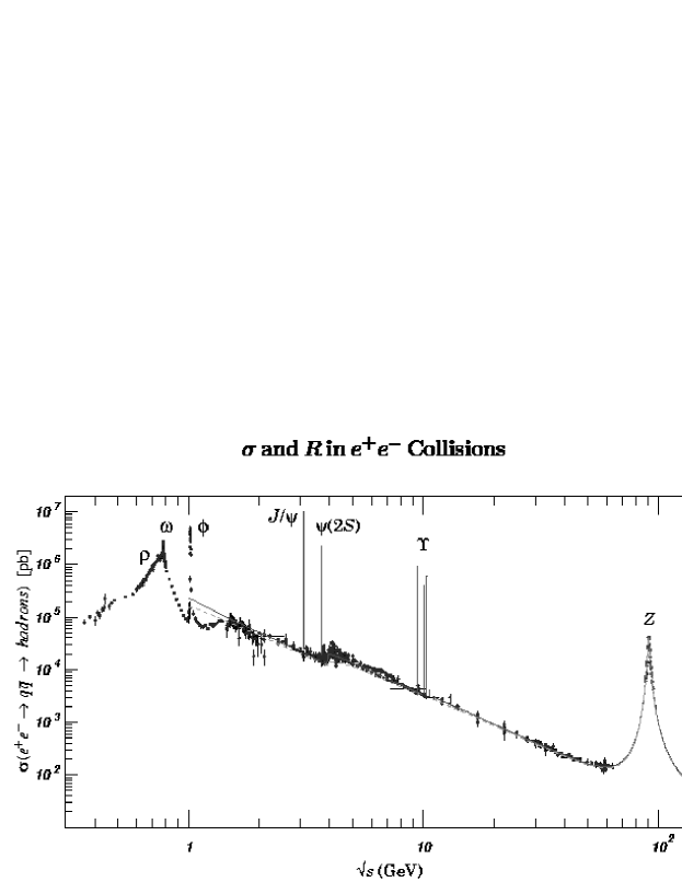
Figure 6: $e^{+}e^{-}$ hadronic cross section (from $\!{}^{{\bf?}}$).

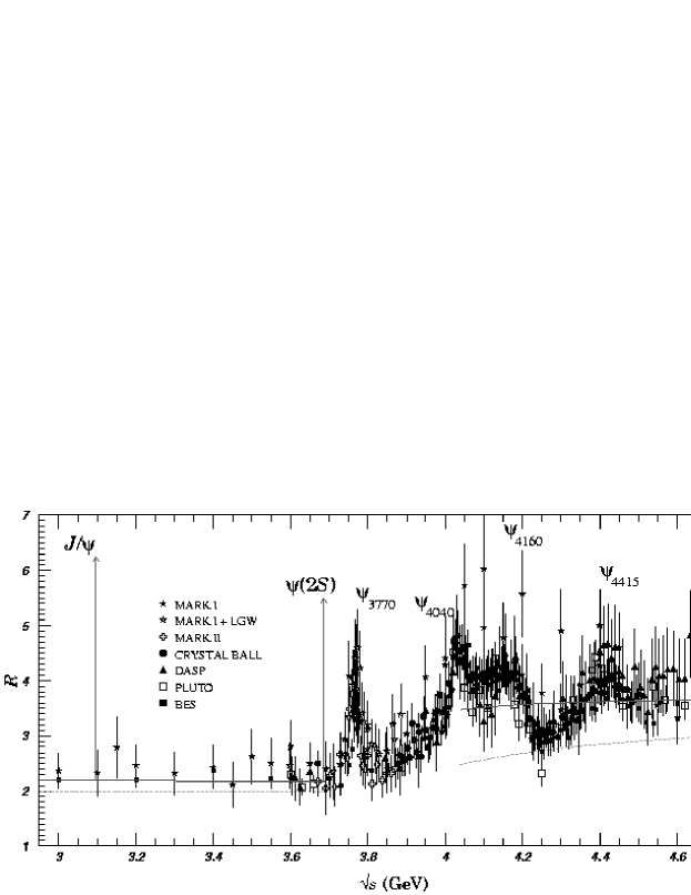
Figure 7: $e^{+}e^{-}\to$ hadrons versus $\mu^{+}\mu^{-}$ in the $c\bar{c}$ region (from $\!{}^{{\bf?}}$).

A closer look reveals additional peaks in the cross sections. These resonaces decay into mesons with open charm like $D^{+}D^{-}$ or $D^{0}\overline{D^{0}}$. Their mass is $D^{\pm}=1870$ MeV and $D^{0}=1865$ MeV, respectively. They carry open charm, their quark content is $c\bar{d}$ and $d\bar{c}$, and $c\bar{u}$ and $u\bar{c}$, respectively, and their quantum numbers are $J^{PC}=0^{-+}$. The states map the Kaon states onto the charm sector.

J/$\psi$ decays to $e^{+}e^{-}$

In J/$\psi$ decays to $e^{+}e^{-}$ the intermediate state is a single virtual photon. This resembles QED in positronium atoms and indeed, one can adopt the transition rate from positronium to $\bar{c}c$ decays. The van Royen Weisskopf equation $\!{}^{{\bf?}}$ reads

$$\Gamma(J/\psi\to e^{+}e^{-})=\frac{16\pi\alpha^{2}Q^{2}}{M_{V}^{2}}|\psi(0)|^{2}$$ (16)

Here $Q^{2}$ is the squared sum of contributing quark charges (see table 2).

Table 2: Photo–coupling of vector mesons.

Meson	wave function	$Q^{2}$
$\rho^{0}$:	$\frac{1}{\sqrt{2}}\left(u\bar{u}-d\bar{d}\right)$	$\left[\frac{1}{\sqrt{2}}\left(2/3-(-1/3)\right)\right]^{2}$	1/2
$\omega$:	$\frac{1}{\sqrt{2}}\left(u\bar{u}+d\bar{d}\right)$	$\left[\frac{1}{\sqrt{2}}\left(2/3+(-1/3)\right)\right]^{2}$	1/18
$\Phi$:	$\left(s\bar{s}\right)$	$\left(1/3\right)^{2}$	1/9
J/$\psi$:	$\left(c\bar{c}\right)$	$\left(2/3\right)^{2}$	4/9

This is an important result: photons couple to $\rho$ (in amplitude) 3 times stronger than to $\omega$. The hypothesis that photons couple to hadrons dominantly via intermediate vector mesons is known as vector meson dominance. As a side remark; the N N $\omega$ coupling is (again in amplitude) $\sim 3.5$ times stronger than the N N $\rho$ coupling.

Charmonium states in radiative decays

In $e^{+}e^{-}$ annihilation, only mesons with quantum numbers $J^{PC}=1^{--}$ are formed. But we also expect charmonium states to exist with other quantum numbers, in particular states with positive $C$–parity. The transitions can be searched for in radiative transitions from the $\psi(2S)$ state. Figure 8 shows the inclusive photon spectrum from the $\psi(2S)$ states $\!{}^{{\bf?}}$. A series of narrow states is seen identifying the masses of intermediate states. The level scheme assigns the lines to specific transitions

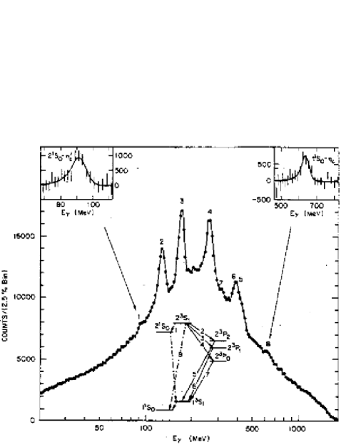
Figure 8: Radiative transitions between charmonium levels (from $\!{}^{{\bf?}}$).

as expected from charmonium models. The width of the lines is given by the experimental resolution of the detector; the charmonium states are produced. The lowest mass state, the $1^{1}S_{0}$ state, is called $\eta_{c}$. It is the $\bar{c}c$ analogue of

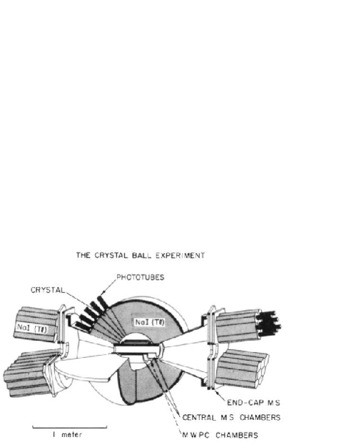
Figure 9: The Crystal Ball detector $\!{}^{{\bf?}}$.

the $\eta$. Its radial excitation is called $2^{1}S_{0}$ or $\eta_{c}^{\prime}$. The small peak assigned to it turned out to be fake in later experiments. The ${}^{3}P_{J}$ states are the lowest–mass $P$-states and are now called $\chi$– or $\chi_{cJ}(1P)$ states. The photons from these transitions were detected in the Crystal Ball detector, a segmented scintillation counter shown in figure 9 which at that time was installed at the SPEAR storage ring.

Charmonium states in $\bar{p}p$ annihilation

Due to the quantum numbers of the virtual photon, $\chi$ states can only be produced, not formed, in $e^{+}e^{-}$ annihilation; formation in this process is restricted to vector mesons. The $\bar{p}p$ annihilation process is much richer due to the finite size and compositeness of the collision partners, hence $\chi$ states can also be observed in a formation experiment. The instrumental width with which a resonance can be seen is limited only by the momentum resolution of the beam and not by the detector resolution. The detector is needed only to identify the number of $\chi$ states. However, $\bar{p}p$ annihilation is dominated by multi–meson final states; the total cross section is on the order of $\sigma_{hadronic}=100mb$. When $\bar{c}c$ states are to be formed, the 3 quarks and antiquarks have to annihilate and then a $\bar{c}c$ pair has to be created. This is an unlikely process, the cross section is correspondingly small, $\sigma_{c\bar{c}}=1\mu b$. Hence, the background below the signal is huge. These problems can be overcome by insisting that the $\bar{c}c$ state should decay into the J/$\psi$ or $\eta_{c}$ which then decays into two electrons or photons, respectively, having a high invariant mass. In this way, the background can be greatly suppressed. The small branching ratio for J/$\psi$ or $\eta_{c}$ decays into the desired final state reduces the rate even further, high count rates are mandatory.

An experiment of this type $\!{}^{{\bf?}}$ was carried out at Fermilab (see figure 10).

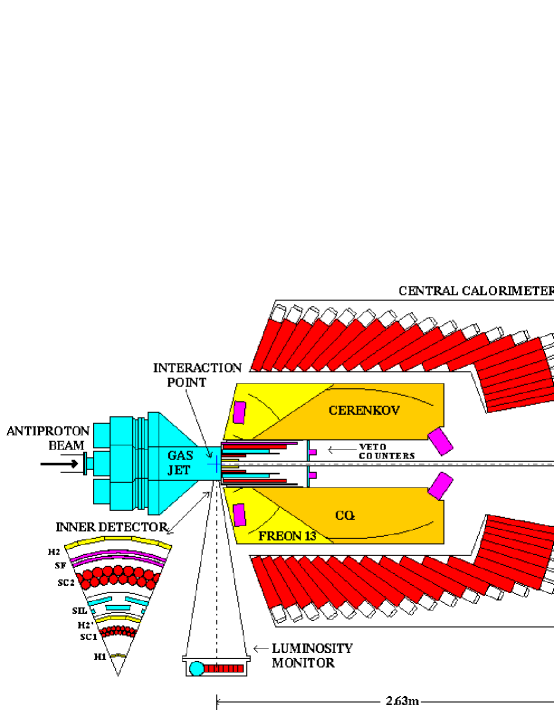
Figure 10: Experiment E760/E835 at FNAL $\!{}^{{\bf?}}$.

Antiprotons were produced by bombarding a target with high–energy protons. The antiprotons are cooled in phase space in a storage ring and are then accelerated to study $\bar{p}p$ collisions at extremely high energies. A fraction of the antiprotons were used for medium–energy physics: $8\cdot 10^{11}$ antiprotons circulated in the Fermilab accumulator ring with a frequency $f_{rev}=0.63$MHz. At each revolution antiprotons are passed through a hydrogen gas jet target, with $\rho_{jet}=3\cdot 10^{14}$H${}_{2}/cm^{3}$, which results in a luminosity $L=N_{\bar{p}}f_{rev}\rho_{jet}$ of $2\cdot 10^{31}$/cm²s. The energy of the antiproton beam, and thus the invariant mass of the $\bar{p}p$ system, can be tuned very precisely according to $\sqrt{s}=m_{p}\cdot\sqrt{2(1+m_{p}E_{\bar{p}})}$. The luminosity is an important concept; the observed rate $R$ of events is related to the luminosity by $R=\sigma\cdot L$. The hadronic background is produced with $R=2\cdot 10^{6}$/s.

Figure 11 shows scans of the $\chi_{c1}(1P)$ and $\chi_{c1}(2P)$ regions. The experimental resolution, given by the precision of the beam momentum, is shown as dashed line. The observed distributions are broader: the natural widths of the states due to their finite life time can now be observed.

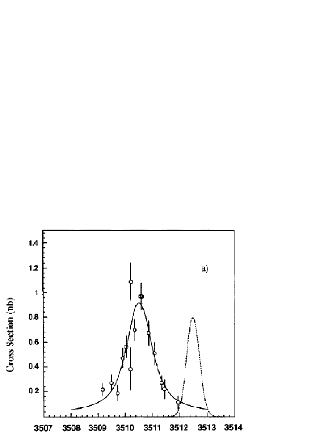
Figure 11: The number of J/$\psi$ as a function of the $\bar{p}p$ mass in the $\chi_{1}$ (a) and $\chi_{2}$ (b) mass regions $\!{}^{{\bf?}}$.

New players at Bejing and Cornell

Charmonium physics came out of the focus of the community. However a new $e^{+}e^{-}$ collider ring was constructed at Bejing, and is

Figure 12: Radiative transitions of the $\psi(2S)$ charmonium state $\!{}^{{\bf?}}$.

producing results. The BES detector measures charged and neutral particles, therefore reactions like $\psi(2S)\rightarrow\gamma\pi^{+}\pi^{-}$ and $\gamma K^{+}K^{-}$ can be studied $\!{}^{{\bf?}}$ (see figure 12). From this data, spin, parities and decay branching ratios of the $\chi$–states can be determined. At present, the $e^{+}e^{-}$ collider ring at Cornell is reduced in energy but upgraded in luminosity and will take data very soon in the charmonium region with extremely high precision.

Figure 13 summarizes the charmonium levels and the transitions between them. The level scheme clearly resembles positronium.

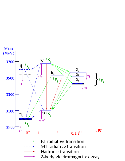
Figure 13: The charmonium level scheme and radiative and hadronic transitions $\!{}^{{\bf?}}$.

1.4 D and B mesons

The charmed quark enriches the spectrum of mesons and baryons by new classes of hadrons with open and hidden charm. Similarly, even more hadrons can be formed with the bottom quark $b$ coming into the play. Mesons with one charmed quark are called $D$-mesons, mesons with one charmed and one strange quark are known as $D_{s}$, and mesons with one bottom quark are $B$-mesons. These have spin $S=0$ and angular momentum $l=0$, and they are pseudoscalar mesons. Vector mesons with $L=0,S=1$ are called $D^{*}$ or $B^{*}$. The $D^{*}_{2}$ has $S=1$ and $L=1$ coupling to $J=2$. Mesons with one bottom and one charmed quark are called $B_{c}$. Mesons with hidden charm are the J/$\psi$, $\psi(2S)$, .., the $\chi_{cJ}(1P)$ states (with $S=1$) or $h_{c}(1P)$ (with $S=0$).

Heavy baryons have been been discovered as well, like the $\Lambda_{c}$ or the $\Lambda_{b}$ with one charmed (bottom) quark, $\Sigma_{c}$ or $\Sigma_{b}$, and so on. These mesons and baryons have very different masses, but the forces between quarks of different flavor are the same ! This can be seen in figure 14.

Figure 14: Flavor independence of the strong forces: Left panel: Mass differences for $L=1$ excitations of mesons and baryons (for systems with aligned spin). Right panel: Mass square differences between PS and V mesons for L=0 octet-decuplet and $L=1$ singlet-octet baryons.

The left panel shows the mass gap for $L=1$ excitations with quark spins aligned, to the $L=0$ meson or baryon ground states (again with aligned quark spins). On the right panel, the ’magnetic’ mass splitting between states with aligned and not aligned spins is plotted. In this case, the differences in mass square are plotted. Note that $M_{1}^{2}-M_{2}^{2}=(M_{1}-M_{2})\cdot(M_{1}+M_{2})$. If this is a constant, $M_{1}-M_{2}$ scales with $1/M$.

1.5 The new states

Exciting discoveries were made last year. Several strikingly narrow resonances were observed, at unexpected masses or with exotic quantum numbers. These were mostly mesons and will be discussed here. Among the new states are two baryon resonance, called $\Theta^{+}(1540)$ and $\Xi^{--}(1862)$. Their discussion is deferred to section 5.

The detectors involved in the discovery of the new meson resonances all provide very good momentum resolution (charged particles are tracked through a magnetic field), photon detection, and particle identification. Even though the correct discrimination of kaons against the pion background or identification of single photons not originating from $\pi^{0}$ decay deserves focused attention, we will assume here that the final state particles are unambiguously identified.

The BABAR resonance

The primary aim of the BABAR (and BELLE) experiments is the study of CP violation in the $b\bar{b}$ system. The colliding $e^{+}e^{-}$ beams produce however many final states; the study reported here was done by searching inclusively (i.e. independent of other particles

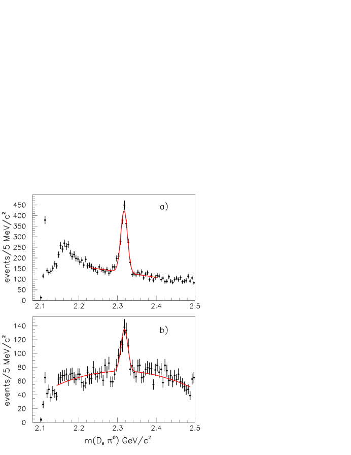
Figure 15: The $D_{s}^{+}\mbox{$\pi^{0}$}$ mass distribution for (a) the decay $D_{s}^{+}\to\rm K^{+}K^{-}\pi^{+}$ and (b) the decay $D_{s}^{+}\to\rm K^{+}K^{-}\pi^{+}\pi^{0}$. The fits to the mass distributions as described in the text are indicated by the curves $\!{}^{{\bf?}}$.

also produced in the same event) for events with two charged kaons, one charged pion, and at 2 or 4 photons which can be combined to one or two $\pi^{0}$. Calculating the $\rm K^{+}K^{-}\pi^{+}$ (or $\rm K^{+}K^{-}\pi^{+}\pi^{0}$) invariant mass reveals contributions from the $D_{s}^{+}$. Then, the $D_{s}^{+}\pi^{0}$ invariant mass spectra are calculated and shown in figure 15. The two spectra refer to two different decay modes of the $D_{s}^{+}$. The fit yields a mass $(2316.8\pm 0.4)$ MeV and $(2317.6\pm 1.3)$ MeV respectively and a width estimated to be less than 10 MeV $\!{}^{{\bf?}}$.

The angular momentum of the $D_{sJ}(2317)^{+}$ is not known but due to its low mass $J=0$ seems to be most likely.

The CLEO resonance

The CLEO collaboration confirmed the $D_{s}^{+}(2317)$ and observed a further $D_{sJ}$ resonance $\!{}^{{\bf?}}$ called $D_{sJ}(2463)^{+}$. The mass difference spectrum $\Delta M(D_{s}^{*}\pi^{0})=M(D_{s}^{*}\pi^{0})-M(D_{s}^{*})$

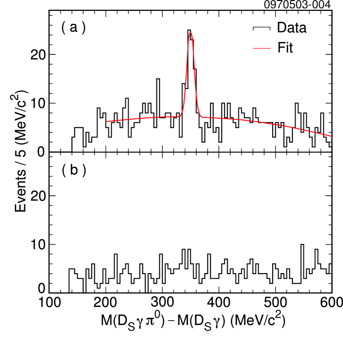
Figure 16: (a) The mass difference spectrum $\Delta M(D_{s}^{*}\pi^{0})=M(D_{s}\gamma\pi^{0})-M(D_{s}\gamma)$ for combinations where the $D_{s}\gamma$ system is consistent with $D_{s}^{*}$ decay (b) The corresponding spectrum where $D_{s}\gamma$ combinations are selected from the $D_{s}^{*}$ side band regions which are defined as $20.8<|\Delta M(D_{s}\gamma)-143.9\,\mbox{MeV/c}^{2}|<33.8\,\mbox{MeV/c}^{2}$ (from $\!{}^{{\bf?}}$).

is shown in figure 16 where the $D_{s}^{*}$ is defined by its $D_{s}\gamma$ decay mode. The signal is kinematically linked to the $D_{sJ}(2317)^{+}$; the two resonances contribute mutually to a peaked background. A correlation study demonstrates the existence of both resonances. The authors argue that, likely, $J=1$.

The BELLE resonance

The BELLE resonance is observed $\!{}^{{\bf?}}$ in the exclusive decay process $B^{\pm}\to\rm K^{\pm}X^{0},X^{0}\to\pi^{+}\pi^{-}J/\psi$. The data was collected with the $e^{+}e^{-}$ beams set to the $\Upsilon(4S)$ resonance which decays into two B mesons.

The beam energy is more precisely known than the momenta of the decay particles. Therefore, B mesons decaying to $\rm K^{+}\pi^{+}\pi^{-}J/\psi$ are reconstructed using the beam-energy constrained mass $M_{\rm bc}$ and the energy difference $\Delta E$

$$M_{\rm bc}\equiv\sqrt{(E_{\rm beam}^{\rm CM})^{2}-(p_{B}^{\rm CM})^{2}}\qquad \qquad\Delta E\equiv E_{B}^{\rm CM}-E_{\rm beam}^{\rm CM},$$ (17)

where $E_{\rm beam}^{\rm CM}$ is the beam energy in the CM system, and $E_{B}^{\rm CM}$ and $p_{B}^{\rm CM}$ are the CM energy and momentum of the $B$ candidate.

Figures 17(a), (b) and (c) show the $M_{\rm bc}$, $M_{\pi^{+}\pi^{-}J/\psi}$, and $\Delta E$ distributions, respectively. The superimposed curves indicate the results of a fit giving a mass of $(3872.0\pm 0.6{\rm(stat)}\pm 0.5{\rm(syst)})$ MeV.

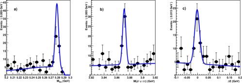
Figure 17: Signal-band projections of (a) $M_{\rm bc}$, (b) $M_{\pi^{+}\pi^{-}J/\psi}$ and (c) $\Delta E$ for the $X(3872)\to\pi^{+}\pi^{-}J/\psi$ signal region with the results of the un-binned fit superimposed $\!{}^{{\bf?}}$.

The result was confirmed at Fermilab by the CDFII collaboration in proton antiproton collisions at $\sqrt{s}=1.96TeV$ $\!{}^{{\bf?}}$.

The BES resonance

At BES a narrow enhancement is observed $\!{}^{{\bf?}}$ in radiative $J/\psi\to\gamma\bar{p}p$ decays. Its mass is very close to $2m_{p}$. No similar structure is seen in $J/\psi\to\pi^{0}\bar{p}p$ decays. Figure 18 shows the $p\bar{p}$ mass distribution without (a) and with (b) phase space correction. The strong contribution at threshold suggests that $p$ and $\bar{p}$ should be in an S-wave. If fit with a Breit Wigner function the peak mass is below $2m_{p}$, at $M=(1859^{~{}+3}_{-10}~{}{\rm(stat)}^{~{}+5}_{-25}~{}{\rm(sys))}~{}{\rm MeV}/c^{2}$, and the total width is $\Gamma<30$ MeV/$c^{2}$ at the 90% confidence level. Since charge conjugation must be positive, the most likely quantum numbers are $J^{PC}=0^{-+}$. The decay angular distribution is not incompatible with this conjecture.

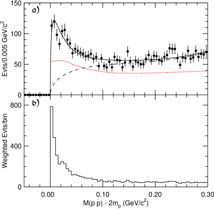
Figure 18: (a) The near threshold $M_{\mbox{$\mbox{p}\bar{\mbox{p}}$}}-2m_{p}$ distribution for the $\gamma\mbox{$\mbox{p}\bar{\mbox{p}}$}$ event sample. The dashed curve is a background function. The dotted curve indicates how the acceptance varies with $\mbox{p}\bar{\mbox{p}}$ invariant mass; the dashed curve shows the fitted background function. (b) The $M_{\mbox{$\mbox{p}\bar{\mbox{p}}$}}-2m_{p}$ distribution with events weighted by $q_{0}/q$ $\!{}^{{\bf?}}$.

Discussion

The two new resonances, $D_{s0}(2317)^{+}$ and $D_{s1}(2463)^{+}$, belong to the family of $D_{sJ}^{+}$ resonances where some members are already known $\!{}^{{\bf?}}$: the pseudoscalar ground state $D_{s}^{+}$ at 1970 MeV, the vector state $D_{s1}^{*}(2112)^{+}$ and two states with orbital angular momentum one, the $D_{s1}(2536)^{+}$ and $D_{s2}(2573)^{+}$. Figure 19 shows the mass spectrum of $D_{sJ}^{+}$ resonances. We expect 2 states with $L=0$ and $S=0$ or $S=1$, and four states with $L=1$ and $S=0$ or $S=1$ where $S=1$ and $L=1$ couple to $J=0,1,2$.

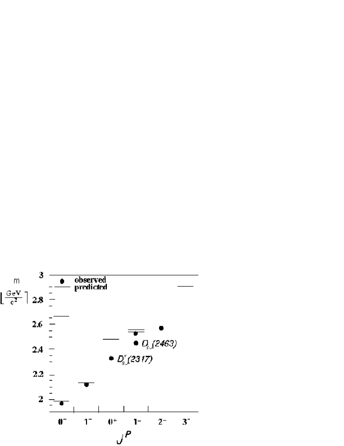
Figure 19: The mass spectrum of $D_{sJ}^{+}$ resonances and their quantum numbers (mostly to be confirmed). The two states ${}^{3}P_{1}$ and ${}^{1}P_{1}$ differ only by their C-parity which is undefined for states with open charm and/or strangeness. Hence the two states mix to form the two mass eigenstates. The predictions of Godfrey and Isgur  $\!{}^{{\bf?}}$ are represented by lines and the data by $\bullet$.

In addition higher mass resonances, radial and higher orbital excitations can be seen to be predicted. The new states do not fit well to the expected masses and there is an intense discussion why the masses of the new mesons are so low. For mesons with one heavy and one light quark one may assume that the light quark spin and orbital angular momenta couple to $j_{\ell}=l_{\ell}+s_{\ell}$, which then couples to the spin of the heavy quark. The heavy quark is supposed to be so heavy that its motion can be neglected. Models based on this assumption are called heavy quark effective theories (HQET). Within this frame the masses can be reproduced reasonably well $\!{}^{{\bf?}}$ but other approaches are certainly not excluded.

The BELLE resonance has a mass of $3872.0$ MeV and is thus far above the $\rm D\bar{D}$ threshold. Its decay mode shows that it is a state with hidden charm, that it contains a $c\bar{c}$ pair. The $\psi(3770)$ has a full width of 24 MeV; the BELLE resonance with its higher mass should be wider. It is not, it is narrow ! This is unexpected. A hint for a solution may lie in the fact that its mass is very close to the $M_{D}+M_{D^{*}}$ mass threshold. There are speculations that the resonance might be a $c\bar{c}g$ state where the $c$ quark and the $\bar{c}$ antiquark couple to a color octet which then is color–neutralized by the gluon field $\!{}^{{\bf?}}$. Such objects are called hybrids.

The BES resonance is a meson with strong coupling to proton plus antiproton. It is narrow,too. It might decay into multi-meson final states with ample phase space but it does not (otherwise it would be a broad resonance). Hence it is interpreted as a $p\bar{p}$ bound state $\!{}^{{\bf?}}$. While $p\bar{p}$ bound states close to the $p\bar{p}$ threshold having very high intrinsic orbital angular momenta might survive annihilation, a narrow state with pseudoscalar quantum numbers seems very unlikely to exist $\!{}^{{\bf?}}$. Th. Walther pointed out that the mass distribution might be faked by bremsstrahlung $\!{}^{{\bf?}}$.

1.6 Baryons

Symmetries play a decisive role in the classification of baryon resonances. The baryon wave function can be decomposed into a color wave function, which is antisymmetric with respect to the exchange of two quarks, the spatial and the spin-flavor wave function. The second ket in the wave function

$$\rm|qqq>=|colour>_{A}\cdot \rm|space;\ spin,flavour>_{S}$$

$$\rm O(6)\qquad SU(6)$$

must be symmetric. The SU(6) part can be decomposed into SU(3)$\otimes$SU(2).

The spatial wave function

The motion of three quarks at positions $r_{i}$ can be described using Jacobean coordinates:

$$\qquad r_{1}-r_{2}$$ (19)

$$\qquad r_{1}+r_{2}-2r_{3}$$ (20)

$$\qquad r_{1}+r_{2}+r_{3}$$ (21)

Equation (21) describes the baryon center–of–mass motion and is not relevant for the internal dynamics of the 3–quark system. There remain two separable motions, called $\rho$ and $\lambda$, where the first one is antisymmetric and the second symmetric with respect to the exchange of quarks 1 and 2.

SU(3) and SU(6)

From now on, we restrict ourselves to light flavors i.e. to $up,down$ and $strange$ quarks. The flavor wave function is then given by SU(3) and allows a decomposition

$$\rm 3\otimes\ 3\otimes\ 3=10_{S}\oplus\ 8_{M}\oplus\ 8_{M}\oplus\ 1_{A},$$ (22)

into a decuplet symmetric w.r.t. the exchange of any two quarks and an antisymmetric singlet and two octets of mixed symmetry. The two octets have different SU(3) structures and only one of them fulfills the symmetry requirements in the total wave functions. Remember that the SU(3) multiplets contain six particle families:

SU(3)	N	$\Delta$	$\Lambda$	$\Sigma$	$\Xi$	$\Omega$
1	no	no	yes	no	no	no
8	yes	no	yes	yes	yes	no
10	no	yes	no	yes	yes	yes

The spin-flavor wave function can be classified according to SU(6).

$$\rm 6\otimes\ 6\otimes\ 6=56_{S}\oplus\ 70_{M}\oplus\ 70_{M}\oplus\ 20_{A}$$ (23)

In the ground state the spatial wave function is symmetric, and the spin-flavor wave function has to be symmetric too. Then, spin and flavor can both be symmetric; this is the case for the decuplet. Spin and flavor wave functions can individually have mixed symmetry, with symmetry in the combined spin-flavor wave function. This coupling represents the baryon octet. The 56-plet thus decomposes into a decuplet with spin 3/2 (four spin projections) plus an octet with spin 1/2 (two spin projections) according to

$$56={{}^{4}}10\ \oplus\ ^{2}8.$$ (24)

Octet and decuplet are schematically presented in figure 20.

Figure 20: Octet and decuplet baryons

The $\Omega^{-}$ was predicted $\!{}^{{\bf?}}$ on the basis of SU(3) by Gell-Mann. Its experimental discovery $\!{}^{{\bf?}}$ was a striking confirmation of SU(3) and of the quark model.

The spin-flavor wave functions can also have mixed symmetry. The 70-plet can be written as

$$70={{}^{2}}10\ \oplus\ {{}^{4}}8\ \oplus\ {{}^{2}}8\ \oplus\ {{}^{2}}1.$$ (25)

Decuplet baryons, e.g. $\Delta^{*}$, in the 70-plet have intrinsic spin 1/2; octet baryons like excited nucleons can have spin 1/2 or 3/2. Singlet baryons with J=1/2, the $\Lambda_{1}$ resonances only exist for spin-flavor wave functions of mixed symmetry. The ground state (with no orbital excitation) has no $\Lambda_{1}$.

The 20-plet is completely antisymmetric and requires an antisymmetric spatial wave function. It is decomposed into an octet with spin 1/2 and a singlet with spin 3/2:

$$20={{}^{2}}8\ \oplus\ {{}^{4}}1.$$ (26)

Regge trajectories

In figure 21 we compare the Regge trajectory for $\Delta^{*}$ resonances having $J=L+3/2$ with the meson trajectory. The offset is given by the $\Delta(1232)$ mass but the slope is the same for both trajectories. Mesons and baryons have the same Regge slope. The QCD forces between quarks and antiquarks are the same as those between quark and diquark. This is an important observation which will be taken up again in section 5.

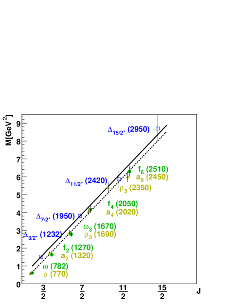
Figure 21: Regge trajectory for $\Delta^{*}$ resonances in comparison to the meson trajectory.

2 Particle decays and partial wave analysis

The aim of an analysis is to determine masses and widths of resonances, their spins, parities and flavor structure.

In the simplest case, a resonance is described by a single–channel Breit-Wigner amplitude; however, a resonance may undergo distortions. The opening of a threshold for a second decay mode reduces the intensity in the channel in study, an effect which is accounted for by use of the Flatte formula. The amplitudes for two resonances close by in masses must not be added; the sum would violate unitarity. Instead, a K–matrix must be used. The partial decay widths to different final states may require the use of multichannel analyses. The couplings of resonances follow SU(2) and SU(3) relations.

Spin and parity of a resonance are reflected in their decay angular distributions. These can be described in the non–relativistic Zemach $\!{}^{{\bf?}}$ or relativistic Rarita-Schwinger $\!{}^{{\bf?}}$ formalism, or using the helicity formalism $\!{}^{{\bf?}}$.

2.1 Particle decays

The transition rate for particle decays are given by Fermi’s golden rule:

$$T_{if}=2\pi|{\cal M}|^{2}\rho(E_{f})$$

$T_{if}$ is the transition probability per unit time. With N particles, the number of decays in the time interval $dt$ is $NT_{if}dt$ or

$$dN=-NT_{if}dt$$

and

$$N=N_{0}e^{-T_{if}t}=N_{0}e^{-(t/\tau)}=N_{0}e^{-\Gamma t}$$

$$\Gamma\tau=\hbar=1$$

The latter equation is the well–known uncertainty principle.

Now we turn to short–lived states in quantum mechanics. Consider a state with energy $E_{0}=\hbar\omega$; it is characterized by a wave function $\psi(t)=\psi_{0}(t)e^{-iE_{0}t}$. Now we allow it to decay:

$\psi\psi=\psi^{*}_{0}(t)\psi_{0}(t)$ $=\psi^{*}_{0}(t=0)\psi_{0}(t=0)e^{-t/\tau}$. Probability density must decay exponentially.

$$\longrightarrow\psi(t)=\psi(t=0)e^{-iE_{0}t}e^{-t/2\tau}$$

A damped oscillation contains more than one frequency. The frequency distribution can be calculated by the Fourier transformation:

$$f(\omega) = f(E)=\int_{0}^{\infty}{\psi(t=0)e^{-iE_{0}t-t/2\tau}}e^{iEt}dt$$

$$= \int_{0}^{\infty}\psi(t=0)e^{-i\left((E_{0}-E)-1/2\tau\right)t}dt\quad=\quad\frac{\psi(t=0)}{\left(E_{0}-E\right)-i/\left(2\tau\right)}$$

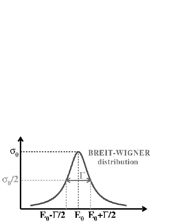
Figure 22: Breit–Wigner resonance.

The probability of finding the energy $E$ is given by

$$f^{*}(E)f(E)=\frac{|\psi(t=0)|^{2}}{\left(E_{0}-E\right)^{2}+1/\left(2\tau\right)^{2}}$$

and, replacing $\tau$ with $1/\Gamma$,

$$\frac{(\Gamma/2)^{2}}{\left(E_{0}-E\right)^{2}+(\Gamma/2)^{2}}$$

gives the Breit–Wigner function. However, resonances are described by amplitudes:

$$BW(E)=\frac{\Gamma/2}{\left(E_{0}-E\right)-i\Gamma/2}=\frac{1/2}{\left(E_{0}-E\right)/\Gamma-i/2}.$$

With

$$2\left(E_{0}-E\right)/\Gamma=\cot\delta:\quad f(E)=\frac{1}{\cot\delta-i}=e^{i\delta}\sin\delta=\frac{i}{2}\left(1-e^{-2i\delta}\right)$$

This formula can be derived from $S$ matrix theory; $\delta$ is called phase shift. The amplitude is zero for $\Gamma/(E-E_{0})<<0$ and starts to be real and positive with a small positive imaginary part. For $\Gamma/(E-E_{0})>>0$ the amplitude is small, real and positive with an small negative imaginary part. The amplitude is purely imaginary $(i)$ for $E=E_{0}$. The phase $\delta$ goes from 0 to $\pi/2$ at resonance and to $\pi$ at high energies.

The Argand circle

The amplitude can be represented conveniently in an Argand diagram (figure 23). The scattering amplitude starts when the real and imaginary part both equal zero. In case of the absence of inelasticities (only elastic scattering is allowed), the scattering amplitude makes one complete circle while the energy runs across the resonance. Inelasticities reduce the amplitude which always stays inside of the circle.

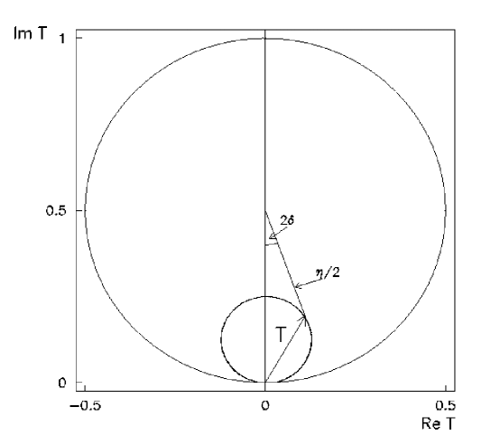
Figure 23: Scattering amplitude T in case of inelastic scattering. Definition of phase $\delta$ and inelasticity $\eta$.

A concrete example $\!{}^{{\bf?}}$ is shown in figure 24: the Argand diagram and cross section for $\pi^{-}p\to\pi^{-}p$ via formation of the N(1650)$D_{1,5}$ resonance (L=2).

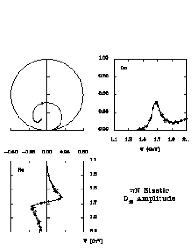
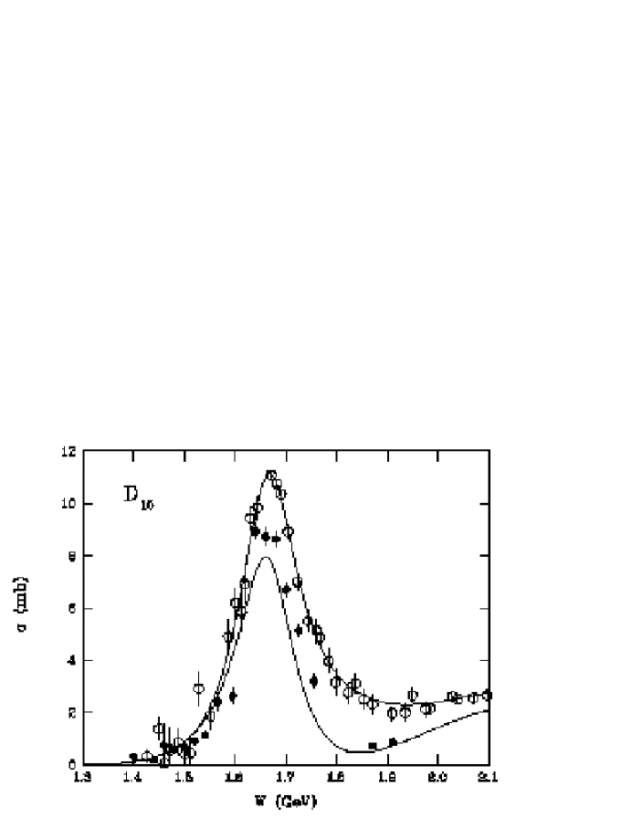
Figure 24: Elastic channel (upper curve), $\pi p\to\pi\pi p$ (lower curve), difference $\pi p\to\eta p$ or $\pi p\to\Lambda$K; from $\!{}^{{\bf?}}$.

The K–matrix

Consider two-body scattering from the initial state i to the final state f, $ab\to cd$. Then

$$\frac{d\sigma_{fi}}{d\Omega}=\frac{1}{(8\pi)^{2}s}\frac{q_{f}}{q_{i}}|{\cal{M}}_{fi}|^{2}=|f_{fi}(\Omega)|^{2}$$

where $s=m^{2}=$ squared CMS energy; q break-up momenta. In case of spins, one has to average over initial spin components and sum over final spin components. The scattering amplitude can be expanded into partial-wave amplitudes:

$$f_{fi}(\Omega)=\frac{1}{q_{i}}\sum(2J+1)T^{J}_{fi}D^{J*}_{\lambda\mu}(\Phi,\Theta,0)$$

One may remove the probability that the particles do not interact by $S=I+iT$. Probability conservation yields $SS^{\dagger}=I$ from which one may define

$$K^{-1}=T^{-1}+iI.$$

From time reversal follows that K is real and symmetric. Below the lowest inelasticity threshold the $S$–matrix can be written as

$$S=e^{2i\delta}\qquad T=e^{i\delta}sin\delta$$

For a two-channel problem, the S-matrix is a $2\times 2$ matrix with

$$S_{ik}S^{*}_{jk}=\delta_{ij}.$$

$$S_{11}=\eta e^{2i\delta_{1}}\qquad S_{22}=\eta e^{2i\delta_{2}}\qquad S_{12}=ie^{i\delta_{1}+\delta_{2}}\sqrt{1-\eta^{2}}.$$

So far, the T matrix is not relativistically invariant. This can be achieved by introducing $\hat{T}$:

$$T_{ij}=\left(\rho_{i}^{\frac{1}{2}}\right)\hat{T}_{ij}\left(\rho_{i})^{\frac{1}{2}}\right)$$

where $\rho_{n}=2q_{n}/m$ are phase space factors. The amplitude now reads

$$\hat{T}^{J}_{fi}(\Omega)=\frac{1}{q_{i}}\sum(2J+1)\hat{T}^{J}_{fi}D^{J*}_{\lambda\mu}(\Phi,\Theta,0)$$

with

$$\rho_{n}=2q_{n}/m=\sqrt{\left[1-\left(\frac{m_{a}+m_{b}}{m}\right)^{2}\right]\left[1-\left(\frac{m_{a}-m_{b}}{m}\right)^{2}\right]}$$

Now the following relations hold:

$$\hat{T}=\frac{1}{\rho}e^{i\delta}sin\delta;\qquad\ \hat{K}^{-1}=\hat{T}^{-1}+i\rho$$

$$\hat{T}=\frac{1}{1-\rho_{1}\rho_{2}\hat{D}-i\left(\rho_{1}\hat{K}_{11}+\rho_{2}\hat{K}_{22}\right)}\left(\begin{array}[]{cc}\hat{K}_{11}-i\rho_{2}\hat{D}&\hat{K}_{12}\\ \hat{K}_{21}&\hat{K}_{22}-i\rho_{1}\hat{D}\end{array}\right)$$

and $\hat{D}=\hat{K}_{11}\hat{K}_{22}-\hat{K}_{12}^{2}$. In case of resonances, we have to introduce poles into the K-matrix:

$$K_{ij}=\sum_{\alpha}\frac{g_{\alpha i}(m)g_{\alpha j}(m)}{m_{\alpha}^{2}-m^{2}}+c_{ij}$$

$$\hat{K}_{ij}=\sum_{\alpha}\frac{g_{\alpha i}(m)g_{\alpha j}(m)}{\left(m_{\alpha}^{2}-m^{2}\right)\sqrt{\rho_{i}\rho_{j}}}+\hat{c}_{ij}$$

The coupling constants g are related to the partial decay widths.

$$g_{\alpha i}^{2}=m_{\alpha}\Gamma_{\alpha i}(m)\qquad\ \Gamma_{\alpha}(m)=\sum_{i}\Gamma_{\alpha i}(m)$$

The partial decay widths and couplings depend on the available phase space,

$$g_{\alpha i}(m)=g_{\alpha i}(m_{\alpha})B^{l}_{\alpha i}(q,q_{\alpha})\sqrt{\rho_{i}}$$

These formulae can be used in the case of several resonances (sum over $\alpha$) decaying into different final states (i). The K–matrix preserves unitarity and analyticity. It is a multi-channel approach.

An example for the use of the K–matrix is shown in figure 25 where two scalar resonances are added, first within the K–matrix formalism (left and center) and then, on the right as a sum of two Breit–Wigner amplitudes. The latter prescription violates unitarity. A more detailed description can be found in $\!{}^{{\bf?}}$.

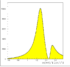
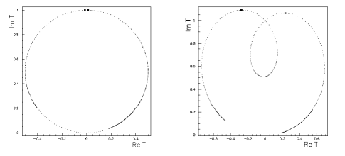
Figure 25: Two close–by resonances added within a K–matrix and as sum of two Breit–Wigner amplitudes (see $\!{}^{{\bf?}}$.

Three-body decays

A particularly important case is that of annihilation into three final-state particles, $M\to(m_{1},m_{2},m_{3})$. The 3 four–momenta define 12 dynamical quantities which are constrained by energy and momentum conservation. The three masses can be determined from a measurement of the particle momenta, and from dE/dx or time–of–flight measurements. Three arbitrary Euler angles define the orientation of the three-body system in space. Hence two variables are needed (and suffice) to be identify the full dynamics. The two variables used to define the Dalitz plot are customly chosen as squared invariant masses ${m_{12}}^{2}$ and ${m_{13}}^{2}$. Then the partial width can be expressed as

$$d\Gamma=\frac{1}{(2\pi)^{3}}\frac{1}{32M}\cdot\overline{|{\cal M}|^{2}}\cdot dm_{12}^{2}dm_{13}^{2}.$$

Events are uniformly distributed in the ($m_{12}^{2},m_{13}^{2}$) plane if the reaction leading to the three particle final state has no internal dynamics. If particles with spin are produced in flight however, the spin may be aligned, the components $m_{j}$ can have a non-statistical distribution and the angular distribution can be distorted.

The Dalitz plot

Events are represented in a Dalitz plot by one point in a plane defined by $m_{12}^{2}$ in x and $m_{23}^{2}$ in the y direction. Since the Dalitz plot represents the phase space, the distribution is flat in case of absence of any dynamical effects. Resonances in $m_{12}^{2}$ are given by a vertical line and those in $m_{23}^{2}$ as horizontal lines. Since

$$m_{13}^{2}=(M_{p}^{2}+m_{1}^{2}+m_{2}^{2}+m_{3}^{2})-(m_{12}^{2}-m_{23}^{2})$$

particles with defined $m_{13}^{2}$ mass are found on the second diagonal.

From the invariant mass of particles 2 and 3

$$m_{23}^{2}=\left(E_{2}+E_{3}\right)^{2}-\left(\vec{p}_{2}+\vec{p}_{3}\right)^{2}$$

we derive

$$m_{23}^{2}=(m_{2}^{2}+m_{3}^{2}+2\cdot E_{2}\cdot E_{3})-(2\cdot|\vec{q}_{2}|\cdot|\vec{q}_{3}|)\cdot\cos\theta$$

with $\theta$ being the angle between $\vec{q}_{2}$ and $\vec{q}_{3}$. This can be rewritten as

$$m_{23}^{2}=\left[\left(m_{23}^{2}\right)_{max}+\left(m_{23}^{2}\right)_{min}\right]+\left[\left(m_{23}^{2}\right)_{max}-\left(m_{23}^{2}\right)_{min}\right]\cdot\cos\theta$$

For a fixed value of $m_{1,2}$ the momentum vector $\vec{p}_{3}$ has a $\cos\theta$ direction w.r.t. the recoil $\vec{p}_{1}$ proportional to $m_{23}^{2}$.

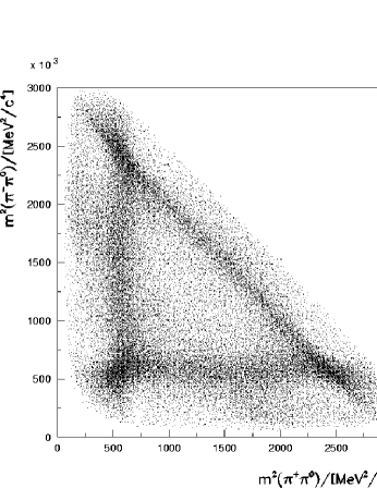
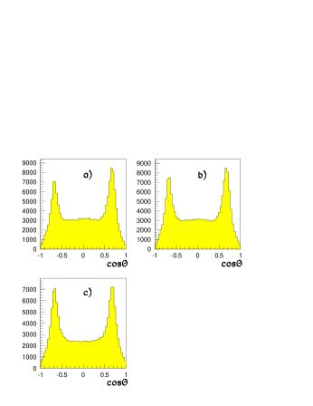
Figure 26: The $\pi^{+}\pi^{-}\pi^{0}$ Dalitz plot in $\rm p\bar{p}$ annihilation at rest, and $\rho^{+}$ (a), $\rho^{-}$ (b) and $\rho^{0}$ (c) decay angular distributions $\!{}^{{\bf?}}$.

The Dalitz plot of figure 26 shows striking evidence for internal dynamics. High-density bands are visible at fixed values of $m_{12}^{2},m_{13}^{2}$, and $m_{23}^{2}$. The three bands correspond to the annihilation modes $\bar{p}p$ $\to$ $\rho^{+}$$\pi^{-}$, $\rho^{-}$$\pi^{+}$, and $\rho^{0}$$\pi^{0}$, respectively. The enhancements due to $\rho$ production as intermediate states are described by dynamical functions $\cal F$.

The three $\rho$ decay angular distributions exhibit two peaks. They are generated by choosing a slice $m_{12}^{2}=m_{\mbox{$\rho^{+}$}}^{2}\pm\Delta m_{\mbox{$\rho^{+}$}}^{2}$  and plotting the number of events as a function of $m_{13}^{2}$. The origin of the peaks in the decay angular distributions is immediately evident from the Dalitz plot. The three bands due to the three $\rho$ charged states cross; at the crossing two amplitudes interfere and the observed intensity increases by a factor of four as one should expect from quantum mechanics. Apart from the peaks the decay angular distribution is approximately given by $\sin^{2}\theta$, hence ${\cal A}\sim\sin\theta$. The three $\rho$ production amplitudes have obviously the same strength indicating that the $\bar{p}p$ initial state(s) from which $\rho$ production occur(s) must have isospin zero.

2.2 Angular distributions

Zemach formalism

Returning to figure 26, the right panel presents decay angular distributions. The $\rho$ is emitted with a momentum $\vec{p}_{\rho}$ and then decays in a direction characterized, in the $\rho$ rest frame, by one angle $\Theta$ and the momentum vector $\vec{p}_{\pi}$. The $\bar{p}p$ initial state has $L=0$; the parity of the initial state is -1 (in both cases), the parities of $\pi$ and $\rho$ are -1. Hence there must be an angular momentum $l_{\rho}=1$ between $\pi$ and $\rho$. This decay is described by the vector $\vec{p}_{\rho}$. The $\rho$ decays also with one unit of angular momentum, with $l_{\pi}=1$. From the two rank-one tensors (=vectors) we have to construct the initial state:

$$\vec{J}=\vec{S}=\left\{\begin{array}[]{ccccc}J&\quad{}^{2s+1}L_{J}&\quad J^{PC}&\quad Zemach&\quad\rm angle\\ 0&\quad{}^{1}S_{0}&\quad 0^{-+}&\quad\vec{p}_{\rho}\cdot\vec{p}_{\pi}&\quad\cos\Theta\\ 1&\quad{}^{3}S_{1}&\quad 1^{--}&\quad\vec{p}_{\rho}\times\vec{p}_{\pi}&\quad\sin\Theta\end{array}\right.$$

For higher spins appropiate operators can be constructed according to the following rules: the operators are

1. traceless: $trace\ t=0$    $\sum t^{i}=0;\qquad\ \sum t^{ii}=0;\qquad\ \sum t^{iii}=0;\ \ldots$

2. symmetric:    $t^{ij}=t^{ji};\qquad\ t^{ijk}=t^{jik}=t^{ij}=t^{ikj}$

3. can be constructed as products of lower-rank tensors   
   $t^{i}t^{j}\Longrightarrow\frac{1}{2}(t^{i}t^{j}+t^{i}t^{j})-\frac{1}{3}t^{2}\delta^{ij}$

4. To reduce rank, multiply with $\delta^{ij}\delta^{kl}$ or $\epsilon^{ijk}$

Helicity formalism

This section is adapted from an unpublished note written by Ulrike Thoma $\!{}^{{\bf?}}$.

The helicity of a particle is defined as the projection of its total angular momentum $\vec{J}=\vec{l}+\vec{s}$ onto its direction of flight.

$$\lambda=\vec{J}\cdot\frac{\vec{p}}{|\vec{p}|}=l\cdot\frac{\vec{p}}{|\vec{p}|}+m_{s}=m_{s}\,\,,$$

Consider a particle A decaying into particles B and C with spins $s_{1}$, $s_{2}$. The particles move along the z-axis (quantization axis). The final state is described by $(2s_{1}+1)\cdot(2s_{2}+1)$ helicity states $\left|p\lambda_{1}\lambda_{2}\right>$; $\lambda_{i}$ are the helicities of the particles and $p$ is their center of mass momentum.

The particle B emitted in a arbitrary direction can be described in spherical coordinates by the angles $\theta$, $\phi$.

Coordinate system for $A\to BC$ decays.

In this case the helicity states are defined in the coordinate system $\Sigma_{3}$ which is produced by a rotation of $\Sigma_{1}$ into the new system.

$$R(\theta,\phi)=\rm{R}_{y2}(\theta)\rm{R}_{z1}(\phi)$$

Using $d$-functions the rotation can be written as

$$D^{J}_{mm^{\prime}}(\theta,\phi)=e^{im^{\prime}\phi}d^{J}_{mm^{\prime}}(\theta)$$

The final states in system $\Sigma_{1}$ can be expressed as

$$\left|p\theta\phi\lambda_{1}\lambda_{2}M\right>_{1}=D^{J}_{M\lambda}(-\theta,-\phi)\cdot\left|p\lambda_{1}\lambda_{2}\right>_{3}$$

with $\lambda=\lambda_{1}-\lambda_{2}$. The transition matrix for the decay is given by

$f_{\lambda_{1}\lambda_{2},M}(\theta,\phi)$	=	$\left<p\theta\phi\lambda_{1}\lambda_{2}M\right|T\left|M^{\prime}\right>$	=	$D^{J\,*}_{M\lambda}(-\theta,-\phi)\left<\lambda_{1}\lambda_{2}\right|T\left|M^{\prime}\right>$
	=	$e^{i\lambda\Phi}d_{\lambda M}^{J}(\theta,\phi)\cdot T_{\lambda_{1}\lambda_{2}}$	=	$D^{J^{\prime}}_{\lambda M}(\theta,\phi)T_{\lambda_{1}\lambda_{2}}\,\,$

The interaction is rotation invariant. The transition amplitude is a matrix with (2$s_{1}$+1)(2$s_{2}$+1) rows and (2$J$+1) columns. $D^{J^{\prime}}_{\lambda M}$($\theta$, $\phi$) describes the geometry, the rotation of the system $\Sigma_{3}$ where the helicity states are defined, back into the CMS system of the resonance; $T_{\lambda_{1}\lambda_{2}}$ describes the dependence on the spins and the orbital angular momenta of the different particles in the decay process. The general form of $T_{\lambda_{1}\lambda_{2}}$ is given by

$$T_{\lambda_{1}\lambda_{2}}=\sum_{ls}\limits\alpha_{ls}\left<J\lambda|ls0\lambda\right>\left<s\lambda|s_{1}s_{2}\lambda_{1},-\lambda_{2}\right>$$

where $\alpha_{ls}$ are unknown fit parameters.

The parameters define the decay spin and orbital angular momentum configuration. The brackets are Clebsch-Gordan couplings for $\vec{J}=\vec{l}+\vec{s}$ and $\vec{s}=\vec{s}_{1}+\vec{s}_{2}$. The sum extends over all allowed $l$ and $s$. Thus:

$$w_{D}(\theta,\phi)=Tr(\rho_{f})=Tr(f\rho_{i}f^{+})$$

where $\rho_{f}$ is the final state density matrix of the dimension (2$s_{1}$+1)(2$s_{2}$+1) and $\rho_{i}$ is the initial density matrix of dimension (2J+1).

Assume that not only A decays into B and C but also B and C decay further into $B_{1}B_{2}$ and $C_{1}C_{2}$. Figure 27 shows a sequential decay of the $\bar{p}$N system. Sequential decays are combined to form one common amplitude. The individual amplitudes are combined as scalar products if they are linked by a line, otherwise by a tensor product. Thus the amplitude is determined to

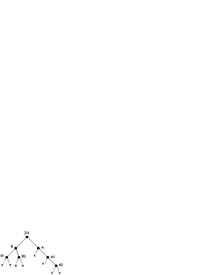
Figure 27: Decay sequence

$$f_{tot}=\left[\,\,(\,\,f(A2)f(A1)f(A)\,\,)\otimes(\,\,[\,\,f(B2)\otimes f(B1)\,\,]\,\,f(B)\,\,)\,\,\right]f(\bar{p}N)\qquad\quad$$

where $\otimes$ represents the tensor product of two matrices. The total helicity amplitude for a reaction $A\to BC$, $B\to B_{1}B_{2}$, $C\to C_{1}C_{2}$, has the form:

$f_{tot}$	=	$\left[f(B)\otimes f(C)\right]f(A)$
	=	$\sum_{{\small\lambda(B)\lambda(C)}}\limits\left[f_{\lambda(B1)\lambda(B2),\lambda(B)}\otimes f_{\lambda(C1)\lambda(C2),\lambda(C)}\right]f_{\lambda(B)\lambda(C),\lambda(A)}$.

The helicity formalism in photo–production processes

In photo–production, a resonance is produced in the process and then decays. We first consider a nucleon resonance that is produced and decays only into two particles, e.g.: $\gamma p\to N^{*}\to p\eta$. The $\gamma p$-system defines the z-axis ($\theta,\phi=0$) and determines the spin density matrix of the $N^{*}$-resonance.

The reaction $\gamma p\to N^{*}$ is related to $N^{*}\to\gamma p$ (which can be calculated using the formalism discussed above) by time reversal invariance. Using

$$f_{\lambda_{c}\lambda_{d},\lambda_{a}\lambda_{b}}(\theta)=(-1)^{\lambda^{\prime}-\lambda}f_{\lambda_{a}\lambda_{b},\lambda_{c}\lambda_{d}}(\theta)\quad\quad$$

valid for $ab\to cd$ with $\lambda^{\prime}=\lambda_{c}-\lambda_{d}$ and $\lambda=\lambda_{a}-\lambda_{d}$, we can write

$$f(\gamma p\to N^{*}\to p\eta)=f(N^{*}\to p\eta)\cdot f^{T}(N^{*}\to\gamma p)$$

Note that $\lambda^{\prime}=\lambda_{N^{*}}=\lambda_{p}-\lambda_{\gamma}$ always holds.

The photo–production amplitude needs to describe the decay of a resonance $R$ $f(R\to N\,X)$ into the channel N X and its production $\gamma p\to R$ calculated using the transposed decay amplitude $f^{T}(R\to p\gamma)$. For photo–production of spin 0 mesons this matrix has the form

$$f^{tot}=\left(\begin{matrix}\left[+\frac{1}{2}\,,-1;+\frac{1}{2}\right]&\left[-\frac{1}{2}\,-1;+\frac{1}{2}\right]&\left[+\frac{1}{2}\,,+1;+\frac{1}{2}\right]&\left[-\frac{1}{2}\,+1;+\frac{1}{2}\right]\cr\left[+\frac{1}{2}\,,-1;-\frac{1}{2}\right]&\left[-\frac{1}{2}\,-1;-\frac{1}{2}\right]&\left[+\frac{1}{2}\,,+1;-\frac{1}{2}\right]&\left[-\frac{1}{2}\,+1;-\frac{1}{2}\right]\cr\end{matrix}\right)$$

where the numbers in the brackets represent [$\lambda_{p},\lambda_{\gamma};\lambda_{p^{f}}$] with $p,\,p^{f}$ being the initial and final state proton. The angular part of the differential cross section is then given by

$$\frac{\rm d\sigma}{\rm d\Omega}=\quad\sim\frac{1}{4}\cdot\sum_{\lambda_{p}\lambda_{\gamma}\lambda^{\prime}}|T(\lambda_{p}\lambda_{\gamma}\lambda_{p^{f}})|^{2}.$$

We now discuss photo–production of the $\rm S_{11}$ and $\rm P_{11}$ resonances and their decay into p$\eta$. The photons are assumed to be unpolarized.

• $S_{11}\to p\eta$

To determine the angular distribution of the decay process the helicity matrix $\rm T_{\lambda_{1}\lambda_{2}}$ has to be calculated,

$$T_{\pm\frac{1}{2},0}=\alpha_{0\,\frac{1}{2}}\left<\,\frac{1}{2},\pm\frac{1}{2}\mid 0,\frac{1}{2};0,\pm\frac{1}{2}\right>\left<\,\frac{1}{2},\pm\frac{1}{2}\mid\frac{1}{2},0;\pm\frac{1}{2},0\right>=\alpha_{0\,\frac{1}{2}}=const.$$

The transition matrix is then given by (the constant is arbitrarily set to 1):

$$f_{\pm\frac{1}{2}\,0,\,M}(\theta,\phi)=\left(\begin{matrix}D^{\frac{1}{2}^{\prime}}_{\frac{1}{2}\,\frac{1}{2}}&D^{\frac{1}{2}^{\prime}}_{\frac{1}{2}\,-\frac{1}{2}}\cr D^{\frac{1}{2}^{\prime}}_{-\frac{1}{2}\,\frac{1}{2}}&D^{\frac{1}{2}^{\prime}}_{-\frac{1}{2}\,-\frac{1}{2}}\cr\end{matrix}\right)$$

where columns represent the spin projections $M_{S_{11}}=\frac{1}{2},\,\,-\frac{1}{2}$ and the rows illustrate $\lambda^{\prime}_{p}=\frac{1}{2},\,\,-\frac{1}{2}$. The z-axis corresponds to direction of flight. The process does not depend on $\phi$. Ee can choose $\phi=0$ and obtain

$$f_{S_{11}\to p\eta}=\left(\begin{matrix}\cos(\frac{\theta}{2})&-\sin(\frac{\theta}{2})\cr\sin(\frac{\theta}{2})&\cos(\frac{\theta}{2})\cr\end{matrix}\right).$$

• $\gamma p\to S_{11}$

First we calculate $S_{11}\to p\gamma$, for $\frac{1}{2}^{-}\to\frac{1}{2}^{+}1^{-}$ and $\ell=0$. Two proton helicities occur $\lambda_{1}=\pm\frac{1}{2}$; the two photon helicities are $s_{2}=1$, $\lambda_{2}=\pm 1\,\,$; $\lambda_{2}=0$ is excluded for real photons. One finds that $\rm T_{\frac{1}{2}\,-1}=T_{-\frac{1}{2}\,+1}=0$, $T_{-\frac{1}{2}\,-1}=-\sqrt{\frac{2}{3}}$, $T_{\frac{1}{2}\,1}=+\sqrt{\frac{2}{3}}$. Setting $\theta$ and $\phi$ to 0 (the $\gamma p$ is parallel to the z-axis), $D_{\lambda\,M}^{J}(0,0)$ is non–zero only for $\lambda=M$.

$$f_{S_{11}\to p\gamma}=\left(\begin{matrix}0&0\cr-\sqrt{\frac{2}{3}}&0\cr 0&\sqrt{\frac{2}{3}}\cr 0&0\cr\end{matrix}\right)$$

The rows correspond to different $\lambda$-values, thus:

$$f(\gamma p\to S_{11})=f^{T}(S_{11}\to p\gamma)=\left(\begin{matrix}0&-\sqrt{\frac{2}{3}}&0&0\cr 0&0&\sqrt{\frac{2}{3}}&0\cr\end{matrix}\right).$$

• $\gamma p\to S_{11}\to p\eta$:

For the whole reaction we obtain

$$f_{\gamma p\to S_{11}\to p\eta}=\left(\begin{matrix}\cos(\frac{\theta}{2})&-\sin(\frac{\theta}{2})\cr\sin(\frac{\theta}{2})&\cos(\frac{\theta}{2})\cr\end{matrix}\right)\cdot\left(\begin{matrix}0&-\sqrt{\frac{2}{3}}&0&0\cr 0&0&\sqrt{\frac{2}{3}}&0\cr\end{matrix}\right)$$

$$\phantom{f_{\gamma p\to S_{11}\to p\eta}}=\left(\begin{matrix}0&-\sqrt{\frac{2}{3}}\cos(\frac{\theta}{2})&-\sqrt{\frac{2}{3}}\sin(\frac{\theta}{2})&0\cr 0&-\sqrt{\frac{2}{3}}\sin(\frac{\theta}{2})&\sqrt{\frac{2}{3}}\cos(\frac{\theta}{2})&0\cr\end{matrix}\right)$$

$${\mathrm{With}}\qquad\qquad\frac{\rm d\sigma}{\rm d\Omega}=\quad\sim\frac{1}{4}\cdot\sum_{\lambda_{p}\lambda_{\gamma}\lambda^{\prime}}|T(\lambda_{p}\lambda_{\gamma}\lambda^{\prime})|^{2}$$

a flat angular distribution is found.

$$\frac{\rm d\sigma}{\rm d\Omega}\sim|A_{S_{11}}|^{2}$$

• $\rm\gamma p\to P_{11}\to p\eta$

The helicity matrix for $P_{11}\to p\eta$ involves the quantum numbers: $\frac{1}{2}^{+}\to\frac{1}{2}^{+}0^{-},\quad\ell=1$ and the matrix elements $T_{\pm\frac{1}{2},0}=\pm\frac{1}{\sqrt{3}}\alpha_{1\,\frac{1}{2}}$. The scattering amplitude is now given by

$$f_{P_{11}\to p\eta}=\left(\begin{matrix}-\frac{1}{\sqrt{3}}\cos(\frac{\theta}{2})&-\frac{1}{\sqrt{3}}(-\sin(\frac{\theta}{2}))\cr\frac{1}{\sqrt{3}}\sin(\frac{\theta}{2})&\frac{1}{\sqrt{3}}\cos(\frac{\theta}{2})\cr\end{matrix}\right)$$

In the next step $P_{11}\to p\gamma$ is calculated ($\frac{1}{2}^{+}\to\frac{1}{2}^{+}1^{-},\quad\ell=1$). Two values for the spin $s$ are possible: $s=\frac{1}{2}$, $s=\frac{3}{2}$. The Clebsch Gordan coefficients depend on $s$ leading to a different $T_{\lambda_{1}\lambda_{2}}$ for the two spins. The D-matrices depend only on $J,\,\lambda$ and $M$, so that they are the same for both cases. One finds
$T_{+\frac{1}{2}\,-1}=T_{-\frac{1}{2}\,+1}=0$ and $T_{-\frac{1}{2}\,-1}=T_{+\frac{1}{2}\,+1}=\alpha_{1\frac{3}{2}}(-\frac{1}{3})+\alpha_{1\frac{1}{2}}(+\frac{\sqrt{2}}{3})=-a$, and

$$f_{\gamma p\to P_{11}}=f^{T}_{P_{11}\to p\gamma}=\left(\begin{matrix}0&-a&0&0\cr 0&0&-a&0\cr\end{matrix}\right)$$

• $\gamma p\to P_{11}\to p\eta$:

For the whole process

$$f_{\gamma p\to P_{11}\to p\eta}=\left(\begin{matrix}0&+\frac{1}{\sqrt{3}}a\,\cos(\frac{\theta}{2})&-\frac{1}{\sqrt{3}}a\,\sin(\frac{\theta}{2})&0\cr 0&-\frac{1}{\sqrt{3}}a\,\sin(\frac{\theta}{2})&-\frac{1}{\sqrt{3}}a\,\cos(\frac{\theta}{2})&0\cr\end{matrix}\right)$$

which leads again to a flat angular distribution; the differential cross section does not depend on $\theta$.

Finally we assume that both resonances are produced; their interference leads to a non-flat angular distribution.

$$f_{\gamma p\to(S_{11}+P_{11})\to p\eta}=\left(\begin{matrix}0&(-\frac{2}{\sqrt{3}}S_{11}+\frac{a}{\sqrt{3}}P_{11})\cos(\frac{\theta}{2})&(-\frac{2}{\sqrt{3}}S_{11}-\frac{a}{\sqrt{3}}P_{11})\sin(\frac{\theta}{2})&0\cr 0&(-\frac{2}{\sqrt{3}}S_{11}-\frac{a}{\sqrt{3}}P_{11})\sin(\frac{\theta}{2})&(\frac{2}{\sqrt{3}}S_{11}-\frac{a}{\sqrt{3}}P_{11})\cos(\frac{\theta}{2})&0\cr\end{matrix}\right).$$

Fir $s=\frac{2}{\sqrt{3}}S_{11}$ and $p=\frac{a}{\sqrt{3}}P_{11}$,

$$\begin{matrix}\frac{\rm d\sigma}{\rm d\Omega}&\,\sim\,&\frac{1}{4}\cdot 2\left[\sin^{2}(\frac{\theta}{2})\cdot|s+p|^{2}+\cos^{2}(\frac{\theta}{2})\cdot|s-p|^{2}\right]\cr&\,\sim\,&|s|^{2}\,+\,|p|^{2}\,-\,2Re(s^{*}p)\cdot\cos(\theta)\cr\end{matrix}.$$

The interference term $2Re(s^{*}p)\cdot\cos(\theta)$ produces a non-flat angular distribution.

2.3 Flavor structure of mesons

Isoscalar coefficients for meson decays

Decays of mesons belonging to one SU(3) multiplet are related by SU(3). The relations are called isoscalar coefficients; they are generalizations of the Clebsch–Gordan coefficients. A restricted set is shown below. Note that $\Sigma$ stands for the SU(3) classification for the isospin triplet system. It can be a $\pi$, $\rho$ or $a_{2}(1320)$. The $\Lambda$ is the symbol for both the singlet and the octet particle. There are three types of transitions needed to describe meson decays into two octet mesons:

$\bf 1\to 8\otimes 8$

$\left(\begin{matrix}\Lambda\end{matrix}\right)$ =

$\left(\begin{matrix}N\bar{K}\ &\ \Sigma\pi\ &\ \Lambda\eta\ &\ \Xi K\end{matrix}\right)$ =

$\frac{1}{\sqrt{8}}\left(\begin{matrix}2\ &\ 3\ &\ -1\ &\ -2\end{matrix}\right)^{1/2}$

$\bf 8_{1}\to 8\otimes 8$

$\left(\begin{matrix}N\ \\ \ \Sigma\ \\ \Lambda\ \\ \ \Xi\ \end{matrix}\right)$ =

$\left(\begin{matrix}\qquad N\pi\ &\ N\eta\ &\ \Sigma K\ &\ \Lambda K\\ N\bar{K}\ &\Sigma\pi\ &\Lambda\pi\ &\Sigma\eta\ &\Xi K\\ \qquad N\bar{K}\ &\ \Sigma\pi\ &\ \Lambda\eta\ &\ \Xi K\\ \qquad\Sigma\bar{K}\ &\ \Lambda\bar{K}\ &\ \Xi\pi\ &\ \Xi\eta\ \\ \end{matrix}\right)$ =

$\left(\begin{matrix}\qquad 9\ &\ -1\ &\ -9\ &\ -1\\ -6\ &0\ &4\ &4\ &-6\\ \qquad 2\ &\ -12\ &\ -4\ &\ -2\\ \qquad 9\ &\ -1\ &\ -9\ &\ -1\ \\ \end{matrix}\right)^{1/2}$

$\bf 8_{2}\to 8\otimes 8$

$\left(\begin{matrix}N\ \\ \ \Sigma\ \\ \Lambda\ \\ \ \Xi\ \end{matrix}\right)$ =

$\left(\begin{matrix}\qquad N\pi\ &\ N\eta\ &\ \Sigma K\ &\ \Lambda K\\ N\bar{K}\ &\Sigma\pi\ &\Lambda\pi\ &\Sigma\eta\ &\Xi K\\ \qquad N\bar{K}\ &\ \Sigma\pi\ &\ \Lambda\eta\ &\ \Xi K\\ \qquad\Sigma\bar{K}\ &\ \Lambda\bar{K}\ &\ \Xi\pi\ &\ \Xi\eta\ \\ \end{matrix}\right)$ =

$\left(\begin{matrix}\qquad 3\ &\ 3\ &\ 3\ &\ -3\\ 2\ &8\ &0\ &0\ &-2\\ \qquad 6\ &\ 0\ &\ 0\ &\ 6\\ \qquad 3\ &\ 3\ &\ 3\ &\ -3\ \\ \end{matrix}\right)^{1/2}$

The $()^{1/2}$ indicates that the square root should be calculated for each matrix element. There are coupling constants defined through the relations:

$$a_{2}(1320)\to\mbox{$\eta$}_{1}\pi=g_{1}\qquad a_{2}(1320)\to\mbox{$\eta$}_{8}\pi=\sqrt{\frac{1}{5}}g_{8}\qquad a_{2}(1320)\to\mbox{$\eta$}_{s\bar{s}}\pi=0$$

from which $g_{1}=-\sqrt{\frac{4}{5}}g_{8}$ can be derived.

The singlet component of the $f_{2}(1270)$ and $f2(1525)$ decays into $\pi\pi,\eta\eta,\eta\eta^{\prime}$, and $\rm K\bar{K}$ with ratios 3:1:0:4. A useful ’rule of thumb’ helps to decide if $8_{1}$ or $8_{2}$ decays should be used; $8_{1}$ is responsible for decays in which the decay of the neutral member of the primary octet into the neutral members of the two octets in the final states are allowed. In this case the product $C^{\prime}$ of the $C$ parities of the neutral members of the three involved octets is positive. $8_{2}$ should be used when $C^{\prime}$ is negative. Examples for $8_{1}$ decays (with $C^{\prime}=1$) are $f_{2}(1270),f2(1525)\to\pi\pi,\eta\eta,\eta\eta^{\prime},\rm K\bar{K}$ or $a_{2}(1320)\to\eta\pi,\rm K\bar{K};\ K_{2}^{*}(1430)\to K\pi,K\eta,K\eta^{\prime}$, $a_{2}(1320)\to\rho\pi$ is an example for $8_{2}$ decays (with $C^{\prime}=-1$).

Table 3: Isoscalar coefficients for decays of mesons with $I=1$ and $I=1/2$.

decay	sym.	antissym.	decay	sym.	antisym.
$\pi\rightarrow\pi\pi$	0	$\frac{\sqrt{2}}{\sqrt{3}}$	$K\rightarrow K\pi$	$\frac{3}{\sqrt{20}}$	$\frac{1}{2}$
$\pi\rightarrow K\bar{K}$	$\frac{1}{\sqrt{6}}$	$\frac{\sqrt{3}}{\sqrt{10}}$	$K\rightarrow K\eta,K\phi$	$\frac{\cos\theta_{\eta}+2\sqrt{2}\sin\theta_{\eta}}{\sqrt{20}}$	$\frac{\cos\theta_{\eta}}{2}$
$\pi\rightarrow\pi\eta,\pi\phi$	0	$\frac{\cos\theta_{\eta}-\sqrt{2}\sin\theta_{\eta}}{\sqrt{5}}$	$K\rightarrow K\eta^{\prime},K\omega$	$\frac{2\sqrt{2}\cos\theta_{\eta}-\sin\theta_{\eta}}{\sqrt{20}}$	$\frac{\sin\theta_{\eta}}{2}$
$\pi\rightarrow\pi\eta^{\prime},\pi\omega$	0	$\frac{\sin\theta_{\eta}+\sqrt{2}\cos\theta_{\eta}}{\sqrt{5}}$

The matrix elements become a bit tedious when final state mesons with mixing angles are involved. With $i$ and $f$ denoting the initial and final state nonet mixing angle, respectively, the SU(3) couplings for $\eta^{\prime}$–, $f_{2}(1270)$– and $\omega$ (dominant $\mbox{u}\bar{\mbox{u}}$ and $\mbox{d}\bar{\mbox{d}}$)–like mesons with nonet mixing are given as

Table 4: Isoscalar coefficients for decays of isoscalar ($\omega$–type) mesons.

decay	symmetric	antisymmetric
$f\rightarrow\pi\pi$	$\sqrt{3}\mbox{$\frac{\sqrt{2}\cos\theta_{f}+\sin\theta_{f}}{\sqrt{10}}$}$	0
$f\rightarrow K\bar{K}$	$\frac{\sin\theta_{f}-2\sqrt{2}\cos\theta_{f}}{\sqrt{10}}$	$\frac{\sin\theta_{f}}{2}$
$f\rightarrow\eta\eta,\phi\phi$	$\frac{-\cos\theta_{\eta}^{2}\sin\theta_{f}-\sqrt{2}(2\sin\theta_{f}\cos\theta_{\eta}\sin\theta_{\eta}-\cos\theta_{f})}{\sqrt{5}}$	0
$f\rightarrow\eta^{\prime}\eta^{\prime},\omega\omega$	$\frac{\sin\theta_{\eta}^{2}\sin\theta_{f}+\sqrt{2}(2\sin\theta_{f}\cos\theta_{\eta}\sin\theta_{\eta}+\cos\theta_{f})}{\sqrt{5}}$	0
$f\rightarrow\eta\eta^{\prime},\phi\omega$	$\frac{\sin\theta_{f}(\sqrt{2}(\cos\theta_{\eta}^{2}-\sin\theta_{\eta}^{2})-\cos\theta_{\eta}\sin\theta_{\eta}}{\sqrt{5}}$	0

while those for $\eta$–, $f^{\prime}_{2}(1525)$– and $\phi$ (dominant $\mbox{s}\bar{\mbox{s}}$)–like mesons read as follows:

Table 5: Isoscalar coefficients for decays of isoscalar ($\Phi$–type) mesons.

decay	symmetric	antisymmetric
$f^{\prime}\rightarrow\pi\pi$	$\sqrt{3}\mbox{$\frac{\sqrt{2}\sin\theta_{f}-\cos\theta_{f}}{\sqrt{10}}$}$	0
$f^{\prime}\rightarrow K\bar{K}$	$\frac{\cos\theta_{f}+2\sqrt{2}\sin\theta_{f}}{\sqrt{10}}$	$\frac{\cos\theta_{f}}{2}$
$f^{\prime}\rightarrow\eta\eta,\phi\phi$	$\frac{-\cos\theta_{\eta}^{2}\cos\theta_{f}-\sqrt{2}(2\cos\theta_{f}\cos\theta_{\eta}\sin\theta_{\eta}+\sin\theta_{f})}{\sqrt{5}}$	0
$f^{\prime}\rightarrow\eta^{\prime}\eta^{\prime},\omega\omega$	$\frac{\sin\theta_{\eta}^{2}\sin\theta_{f}+\sqrt{2}(2\sin\theta_{f}\cos\theta_{\eta}\sin\theta_{\eta}+\cos\theta_{f})}{\sqrt{5}}$	0
$f^{\prime}\rightarrow\eta\eta^{\prime},\phi\omega$	$\frac{\cos\theta_{f}(\sqrt{2}(\cos\theta_{\eta}^{2}-\sin\theta_{\eta}^{2})-\cos\theta_{\eta}\sin\theta_{\eta}}{\sqrt{5}}$	0

The names in the tables are generic, i.e. $f^{\prime}$ stands for $\Phi_{3}$, $f_{4}^{\prime}$ and so on.

Fits

We now ask if the SU(3) isoscalar coefficients are as useful as the Clebsch–Gordan coefficients proved to be. For this purpose we apply the matrix elements to relate tensor decays into two pseudoscalar mesons and decays into a vector and a pseudoscalar meson. The former transitions are of type $C^{\prime}=1$, the latter ones of type $C^{\prime}=-1$.

The matrix element $\cal M$

$$d\Gamma=\frac{1}{32\pi^{2}}|{\cal M}|^{2}\frac{q}{m^{2}}d\Omega$$

contains a coupling constant, $C_{T\mbox{$\rightarrow$}PS+PS}$ or $C_{T\mbox{$\rightarrow$}V+PS}$ (which is calculable in dynamical models), the SU(3) amplitudes $c_{isoscalar}$ and a dynamical function $F(q)$ with $q$ being the breakup momentum.

$$B_{2}(qR)=\sqrt{\frac{13(qR)^{2}}{9+3(qR)+9(qR)^{2}}}$$

$$BW(m)=\frac{m_{0}\Gamma_{0}}{m^{2}-m_{0}^{2}-im_{0}\Gamma_{0}}\$$

Decay	Data				Fit		$\chi^{2}$
	$\Gamma$		$\sigma_{\Gamma}$		$\Gamma$
$a_{2}\mbox{$\rightarrow$}\pi\eta$	15.	95 $\pm$	1.	32	24.	8	2.	99
$a_{2}\mbox{$\rightarrow$}\pi\eta^{\prime}$	0.	63 $\pm$	0.	12	1.	2	4.	39
$a_{2}\mbox{$\rightarrow$}K\bar{K}$	5.	39 $\pm$	0.	88	5.	2	0.	01
$f_{2}\mbox{$\rightarrow$}\pi\pi$	157.	0 $\pm$	5.	0	117.	1	2.	77
$f_{2}\mbox{$\rightarrow$}K\bar{K}$	8.	5 $\pm$	1.	0	8.	0	0.	08
$f_{2}\mbox{$\rightarrow$}\eta\eta$	0.	8 $\pm$	1.	0	1.	5	0.	44
$f^{\prime}_{2}\mbox{$\rightarrow$}\pi\pi$	4.	2 $\pm$	1.	9	3.	7	0.	07
$f^{\prime}_{2}\mbox{$\rightarrow$}K\bar{K}$	55.	7 $\pm$	5.	0	48.	6	0.	43
$f^{\prime}_{2}\mbox{$\rightarrow$}\eta\eta$	6.	1 $\pm$	1.	9	5.	3	0.	12
$f^{\prime}_{2}\mbox{$\rightarrow$}\eta\eta^{\prime}$	0.	0 $\pm$	0.	8	0.	7	0.	77
$K_{2}\mbox{$\rightarrow$}K\pi$	48.	9 $\pm$	1.	7	61.	1	0.	99
$K_{2}\mbox{$\rightarrow$}K\eta$	0.	14 $\pm$	0.	28	0.	2	0.	02

Decay	Data				Fit		$\chi^{2}$
	$\Gamma$		$\sigma_{\Gamma}$		$\Gamma$
$a_{2}\mbox{$\rightarrow$}\pi\rho$	77.	1 $\pm$	3.	5	66.	0	0.	67
$f_{2}\mbox{$\rightarrow$}K^{*}\bar{K}$	0.	0 $\pm$	1.	8	0.	2	0.	01
$f^{\prime}_{2}\mbox{$\rightarrow$}K^{*}\bar{K}$	10.	0 $\pm$	10.	0	11.	8	0.	03
$K_{2}\mbox{$\rightarrow$}K\rho$	8.	7 $\pm$	0.	8	11.	5	1.	29
$K_{2}\mbox{$\rightarrow$}K\omega$	2.	7 $\pm$	0.	8	1.	0	0.	00
$K_{2}\mbox{$\rightarrow$}K^{*}\pi$	24.	8 $\pm$	1.	7	24.	1	0.	02
$K_{2}\mbox{$\rightarrow$}K^{*}\eta$	0.	0 $\pm$	1.	0	0.	9	0.	81

Results of the final fit. The $\chi^{2}$ values

include 20% SU(3) symmetry breaking.

Obviously tensor meson decays are nearly compatible with SU(3). One has to assume 20% symmetry breaking to achieve a fit with $\chi^{2}/N_{F}\sim 1$. From the fit nonet mixing angles can be determined. They are not inconsistent with the values obtained from the Gell-Mann–Okubo mass formula.

$$\begin{matrix}\Theta_{ps\ }&=&-(14.4\pm\ 2.9)^{\circ}&\qquad\ &R&=&0.2\pm\ 0.04\,fm\cr\Theta_{vec}\ &=&+(37.5\pm\ 8.0)^{\circ}&&C_{T\mbox{$\rightarrow$}PS+PS}&=&1.11\pm 0.05\cr\Theta_{ten}\ &=&+(28.3\pm\ 1.6)^{\circ}&&C_{T\mbox{$\rightarrow$}PS+V\ }&=&2.07\pm 0.13\cr\lambda\ &=&0.77\pm\ 0.10&&&&\cr\end{matrix}$$

SU(3) is broken; the chance of producing an $\bar{s}s$ pair out of the vacuum is reduced by $0.77\pm\ 0.10$ compared to the chance of producing a light $\bar{q}q$ pair. The matrix elements and fits are taken from $\!{}^{{\bf?}}$.

3 Particles and their interaction

3.1 The particles: quark and leptons

Quarks and leptons are the basic building blocks of matter. These particles have spin 1/2 and are fermions fulfilling the Pauli principle which states: the wave functions of two identical fermions must be antisymmetric with respect to their exchange. Fermions interact via exchange of bosons, with spin 0 (e.g. pions in nuclear physics), spin 1 (photons, gluons, vector mesons, weak interaction bosons) or spin 2 (gravitons, tensor mesons).

Leptons

Table 6 lists charged ($e^{-},\mu^{-},\tau^{-}$) and neutral ($v_{e},\nu_{\mu},\nu_{\tau}$) leptons. All leptons (and all quarks) have their own antiparticles. Fermions and antifermions have two spin components but weak interaction couples only to left–hand currents of fermions and to the right–hand currents of antifermions. The separate conservation of the 3 lepton numbers is deduced from, e.g., the absence of electrons in a beam of high energy neutrinos originating from $\pi^{-}\to\mu^{-}\nu$ decays, or from the non-observation of $\tau^{-}\to e^{-}\gamma$ decays. We now know that the 3 generations are mixed, i.e. that the mass eigenstates are not identical with the weak–interaction eigenstates.

Table 6: Leptons and their quantum numbers.

Classification	$e^{-}/\nu_{e}$	$\mu^{-}/\nu_{\mu}$	$\tau^{-}/\nu_{\tau}$
e-lepton number	1	0	0
$\mu$-lepton number	0	1	0
$\tau$-lepton number	0	0	1

Quarks and their quantum numbers

Quarks have charges of 2/3 or -1/3 and not 1 (in units of the positron charge $e$). Additionally quarks carry a new type of charge, called color, in 3 variants defined to be red, blue, and green. Antiquarks have the complementary colors anti-red, anti-blue, and anti-green. Mesons composed of a quark and an antiquark can be written as superposition (in the quantum mechanical sense) $q_{red}\overline{q_{red}}+q_{blue}\overline{q_{blue}}+q_{green}\overline{q_{green}}$, and baryons as $q_{red}q_{blue}q_{green}$. Color and anti-color neutralize and so do three colors or three anti-colors.

Table 7: Quarks and their quantum numbers

Classification	$d$	$u$	$s$	$c$	$b$	$t$
Charge	-1/3	2/3	-1/3	2/3	-1/3	2/3
Isospin $I$	1/2	1/2	0	0	0	0
$I_{3}$	-1/2	1/2	0	0	0	0
Strangeness $s$	0	0	-1	0	0	0
Charm $c$	0	0	0	1	0	0
Beauty (bottom) $b$	0	0	0	0	-1	0
Truth (top) $t$	0	0	0	0	0	1

All quantities like strangeness $s$ or topness $t$ except the isospin $I$ change sign when a particle is replaced by its antiparticle. The sign of the flavor in Table 7 is given by the sign of the meson charge. Examples: Charge(K⁺) = Charge($u{\bar{s}}$) = +1      Strangeness of $\bar{s}$: $S=1$ Charge(D⁺) = Charge(${c}\bar{d}$) = +1      Charm of $c$: $C=1$ Charge(B^-) = Charge(${b}\bar{u}$) = -1      Beauty of $b$: $B=-1$

The masses of quarks are much more difficult to determine. Even the concept of a quark mass is difficult to understand. No free separated quark has ever been observed; quarks are confined and we cannot make a quark mass measurement. What we can do is construct a model for mesons and baryons as being composed of two or three constituent quarks. We may guess an interaction and then hope that for a good choice of quark masses there is approximate agreement between model and experiment. In this way we determine constituent quark masses. Or we may try to solve the theory of strong interactions (to be outlined below). For the full theory, we have no chance except for very high momentum transfer (perturbation theory) or in the framework of effective field theory at very low momenta (chiral perturbation theory). The quark masses enter these calculations as parameters which can then be determined by comparison of the computational results with data. In this case, we solve the equations of strong interactions and the resulting quark masses are called current quark masses. In table 8, mean values $\!{}^{{\bf?}}$ are given.

Table 8: Constituent and current quark masses

Quark masses:
Classification	$d$	$u$	$s$		$c$	$b$	$t$
Current mass	$\sim$6	$\sim$ 3	$\sim$115	MeV	$\sim$1.2	$\sim$4.2	$\sim$174	GeV
Constituent mass	$\sim$340	$\sim$340	$\sim$510	MeV	$\sim$1.2	$\sim$4.2	$\sim$174	GeV

3.2 Quarks and leptons and their interactions

The Standard Model and QCD

Within the Standard Model we have 6 leptons and 6 quarks with different flavors (see figure 28). They interact via exchange of photons or of the 3 weak interaction bosons $W^{\pm},Z^{0}$. This part of the interaction is called quantum flavor dynamics; it unifies quantum electrodynamics and weak interactions. The four vector bosons ($\gamma,W^{\pm},Z^{0}$) couple to the electric and weak charges but not to color. Quarks carry a further charge, color, and interact in addition via the exchange of gluons. Color is triple valued; all objects directly observable in experiments are color–neutral. Gluons can be thought to carry one color and one anticolor in a color octet configuration; the completely symmetric configuration $1/\sqrt{3}(\bar{r}r+\bar{b}b+\bar{g}g)$ is a color singlet and excluded, hence there exist 8 gluons. The gauge group of strong interactions is thus $SU_{C}(3)$. Likewise the gauge group of weak interaction is $SU(2)$ and $U(1)$ the gauge group of QED.

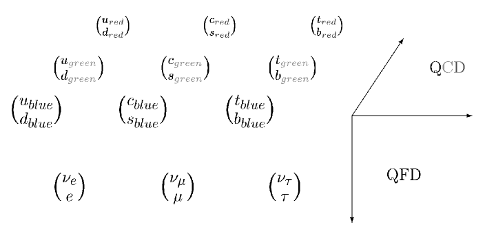
Figure 28: Particles and interactions in the Standard Model.

The Standard Model can be broken into its components:

$SU_{C}(3)$	$\otimes$	$SU(2)$	$\otimes$	$U(1)$
$\Downarrow$		$\Downarrow$		$\Downarrow$
8 gluons		$W^{\pm},Z^{0}$		photon
strong interactions		electro-weak interactions

Gluons are massless particles like photons. It is unclear if the notion of a constituent gluon mass (from an effective parameterization of gluon self–interactions) is meaningful. Sometimes a constituent mass of 700 MeV is assigned to them. Gluons carry the same quantum numbers as photons, $J^{PC}=1^{--}$. Unlike the electrically neutral photons, they carry color. Not only quarks and gluons interact; gluon–gluon interactions are possible as well with three– and four–point vertices.

A theory of strong interactions based on the exchange of colored gluons between colored quarks can be constructed in analogously to quantum electro dynamics. It was a great success that the resulting theory, quantum chromo dynamics, can be shown to be renormalizable. Like in QED, some expressions give infinite contributions, but the renormalization scheme allows one to control all divergencies. The color-electromagnetic fields

$$F_{\mu\nu}^{a}=\delta_{\mu}A_{\nu}^{a}-\delta_{\nu}A_{\mu}^{a}+g_{s}f_{abc}A_{\mu}^{b}A_{\nu}^{c}$$

resemble QED very much, except for the color indices $a,b$, and $c$ and the third term describing gluon–gluon interactions.

The beauty of QCD as a theory of strong interactions has some ugly spots. The coupling constant $\alpha_{s}$ increases dramatically with decreasing momentum transfer, and QCD predictions in the low–energy regime are (mostly) not possible. Only at high momentum transfer is $\alpha_{s}$ small and does QCD become a testable and useful theory. Numerically, there is progress to calculate QCD quantities on a discrete space–time lattice. Figure 29 shows as example the static $Q\bar{Q}$ potential as a function of separation $\!{}^{{\bf?}}$. It is the potential energy between two heavy quarks; the possibility that virtual $\bar{q}q$ pairs can be created is neglected. The line represents a superposition of a $1/r$ potential as expected from one–gluon exchange between quarks and a linearly rising part reflecting confinement.

Figure 29: The potential energy between two heavy quarks (with fixed positions) as a function of their separation from lattice QCD. The solid line represents a potential in the form $V(r)=\frac{4}{3}\frac{\alpha_{s}}{r}+b\cdot r$; from  $\!{}^{{\bf?}}$.

From large energies to large distances

Figure 30 sketches the situation. At very large energies QCD can be treated perturbatively. The strong interaction constant $\alpha_{s}$ decreases and particles behave asymptotically as if they were free. For lower $Q^{2}$ confinement becomes the most important aspect of strong interactions. This is the realm of non–perturbative QCD or of strong QCD. At very small $Q^{2}$, in the chiral limit, observables can be expanded in powers of masses and momenta and chiral perturbation theory leads to reliable predictions $\!{}^{{\bf?}}$. In an extremely hot and dense environment we expect quarks to become free; a phase transition to the quark–gluon plasma is expected $\!{}^{{\bf?}}$ and has likely been observed $\!{}^{{\bf?}}$.

The region of interest here is the one where QCD is really strong, where perturbative QCD and chiral perturbation theory both fail. This is the region most relevant to our daily life; in this region protons and neutrons and their excitations exist. For momentum scales given by typical hadron masses, not only $\alpha_{s}$ changes but also the relevant degrees of freedom change from current quarks and gluons to constituent quarks, instantons and vacuum condensates. To understand this transition is one of the most challenging intellectual problems.

Figure 30: QCD observables as a function of $Q^{2}$.

Basic questions in strong QCD

A clarification of the following central issues is needed:

• What are the relevant degrees of freedom that govern hadronic phenomena ? The relevant degrees of freedom in superconductors are Cooper pairs and not electrons. In meson and baryon spectroscopy, the constituent quarks seem to play an important role, but how are they formed and what is their interaction ?

• What is the relation between partonic degrees of freedom in the infinite momentum frame and the structure of hadrons in the rest frame ? At large momentum transfers we know that about 50% of the momentum of a proton is carried by gluons and not by quarks. In deep inelastic scattering structure functions reveal the importance of sea quarks. Do these participate in the dynamics of mesons and baryons and, is so, how ?

• What are the mechanisms for confinement and for chiral symmetry breaking ? Are deconfinement and chiral symmetry restoration linked and can precursor phenomena be seen in nuclear physics ? At very large densities and temperatures, quarks can no longer be assigned to a particular proton; quarks can be exchanged frequently and propagate freely in this dense material, conserving chirality. This is a phase transition from the regime of broken chiral symmetry to a regime were it is restored; and from the hadronic phase to the quark–gluon plasma. It is unknown whether these two phase transitions are identical, occurring under the same conditions.

Modeling strong QCD

The answers to these questions will not be the direct result of experiments. Models are needed to link observables to these fundamental questions. Significant observables are the nucleon excitation spectrum and their electromagnetic couplings including their off-shell behavior and the response of hadronic properties to the exposure by a nuclear environment.

For many physicists the ultimate hope of ’solving’ QCD is performing numerical calculations on a space–time lattice. At least for the years to come we have to rely on models. These models try to shape what we know or believe about QCD; they are called QCD inspired models.

Gluon exchange and the flux tube model

A very popular version introduces a linear confinement potential and a kind of ’effective’ one-gluon exchange (with $\alpha_{s}$ chosen arbitrarily and neglecting higher orders of an expansion in $\alpha_{s}$). Flux tube models concentrate the gluon field connecting a quark and an antiquark in a tube of constant energy density. The flux tube introduces a new degree of freedom into hadrons; while the orbital angular momentum along the direction between $e^{+}$ and $e^{-}$ in positronium vanishes, the flux tube can rotate around this axis. This dynamical enrichment leads to a richer spectrum. The additional states are called hybrids.

Chiral symmetry and instanton–induced interactions

The $u,d$,and $s$ quarks are nearly massless; the so–called “current” quark masses (.i.e. those which appear in the fundamental QCD Lagrangian) are in the mass range, respectively, from 1.5 to 5 MeV; 3 to 9 MeV, or 60 to 170 MeV $\!{}^{{\bf?}}$. In the chiral limit QCD possesses a large symmetry, and quarks with vanishing mass preserve their handiness, their chirality. If chiral symmetry were unbroken, all baryons would appear as parity doublets. Obviously this is not the case since the masses of proton and its first orbital–angular momentum excitation N(1535)S₁₁ are very different. Hence the (approximate) chiral symmetry is broken spontaneously. As a result the eight pseudoscalar mesons $\rm\pi,K$, and $\eta$ are light Goldstone bosons. They are light but not massless (as the Goldstone therorem  $\!{}^{{\bf?}}$ would require) because the current quarks have small (but finite) masses.

Compared to the proton or $\Lambda$, the 8 pseudoscalar mesons $\pi,\eta$ and K have small masses; their masses are remnants of the Goldstone theorem. Now we have a problem. The $\eta^{\prime}$ mass is close to the proton mass, but due to flavor $SU(3)$, or $SU_{F}(3)$, it should have a small mass too but it has not. As an $SU_{F}(3)$ singlet it couples directly to the gluon fields. This gives rise to an additional interaction introduced by ’t Hooft $\!{}^{{\bf?}}$. It originates from the spontaneously broken chiral symmetry and the occurance of instantons in the QCD vacuum $\!{}^{{\bf?},{\bf?},{\bf?}}$. Their action on the masses of pseudoscalar and scalar mesons can be seen in figure 31 $\!{}^{{\bf?}}$).

Instanton–induced interactions originate from vacuum fluctuations of the gluon fields. Already in QED there are vacuum fluctuations of the electromagnetic fields. Unlike QED, QCD allows solutions to have “topological charge” or a “winding number” (I like to interprete theses as field vortices since they can flip quark spins; technically, QCD vortices are different objects and may have non–integer winding numbers).

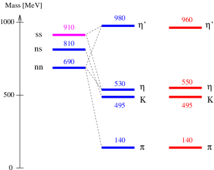
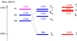
Figure 31: The action of instantons in the mass spectrum of pseudoscalar (left) and scalar (right) mesons. Shown are the spectra as calculated using only a confinement potential and the mass shifts resulting from instantons (from $\!{}^{{\bf?}}$).

Quarks can flip helicity when scattering on instanton fluctuations. Instantons change quark helicity from right to left, anti–instantons from left to right. Therefore, when quarks scatter on many instantons and anti–instantons they acquire a dynamical mass signaling the spontaneous breaking of chiral symmetry.

These induced spin–flips are the origin of the instanton–induced interactions. The same interaction acts independently on $u,d$, and $s$ quarks so that each of them flip helicity. Averaging over the positions of the instanton fluctuation induces a correlation between the $u,d$, and $s$ quarks, which can be written conventiently in the form of the ’t Hooft interaction. Instanton–induced interactions violate the OZI rule. In mesons, a quark can flip its spin only when the antiquark flips its spin simultaneously since the total spin is conserved. $J$ is conserved, too. Thus $J$ must vanish, and instanton–induced interactions contribute only to pseudoscalar and scalar mesons. In baryons, spin and flavor flips can only occur when the two–quark wave function is antisymmetric in spin and in flavor $\!{}^{{\bf?}}$ when the two quarks are exchanged. In baryons with a total quark spin 1/2, the $(qq)$–spin vanishes for one component of the baryonic wave function, and this component is antisymmetric. In octet baryons one $(qq)$ is antisymmetric in flavor. In singlet baryons all three $(qq)$ pairs are antisymmetric w.r.t. their exchange.

Due to spontaneous symmetry breaking, the isovector $q\bar{q}$ pairs in ${}^{3}S_{1}$ acquire the $\rho$ mass; the pion remains massless. However there is a second kind how chiral symmetry is broken. The massless quarks couple, like leptons, to the Higgs field which generates the current quark masses. The current quark mass then gives a finite mass to the pion. Chiral symmetry leads to constituent quarks and is responsible for the largest fraction of the proton mass.

The situation can be compared to the more familiar magnetism. Individual Fe atoms have a magnetic moment and their directions are arbritrary. Many Fe atoms cluster to the Weiss districts with a macroscopic magnetization in a fixed direction. The direction is random; even though the atoms within the Weiss district have no ’reason’, they decide spontaneously to magnetically point in a specific direction. An external magnetic field may induce a preferred direction; this is an induced (external) breaking of rotational symmetry.

The chiral soliton model

The concept of a nucleon composed of 3 constituent quarks is certainly oversimplified and the hadronic properties of nucleons cannot be understood or, at least, are not understood in terms of quarks and their interactions. Skyrme studied the pion field and discovered that by adding a non–linear “$\sigma$ term” to the pion field equation, stable solutions can result $\!{}^{{\bf?}}$. These solutions have half integer spin and a winding number identified by Witten $\!{}^{{\bf?}}$ as the baryon number. These stable solutions of the pion field equation are called soliton solutions.

Of course the Skyrme model does not imply that there are no quarks. Again we compare the situation with magnetic interactions. The theory of ferromagnetism does not imply that Weiss districts are elementary physics. The Skyrme view can be used to understand aspects of baryons from a different point of view. In a modification of the Skyrme model, in the chiral soliton model $\!{}^{{\bf?}}$, the Skyrme solitons tur out to be the self–consistent field that binds quarks inside a baryon.

Figure 32: Quarks and sea quarks are dynamically coupled. The equations of motion support soliton solutions which can be organized into multiplets. The lowest lying multiplets are ${\bf 8}$ and ${\bf 10}$ and $\bf\overline{10}$.

Translated into the quark language, the baryon does not consist only of 3 quarks but there are also sea quarks. If $q\bar{q}$ pairs are assembled in light chiral fields, it costs little additional energy to produce the pairs, provided their flavor content is matched to the quantum numbers of the baryon. Baryons are never three–quark states; there is always an admixture of additional $q\bar{q}$ pairs. Thus, not only octet and decuplet baryons are to be expected, but also higher multiplets.

In the Skyrme model spin and isospin are coupled and we expect ’rotational bands’ with $I=J$. Indeed, octet baryons have $J=1/2$ and $I=1/2$, and decuplet baryons coorespond to $J=3/2$ and $I=3/2$. We should expect a multiplet with $J=5/2$ and $I=5/2$ but baryons with isospin 5/2 have never been found. Such states would be expected as members of a higher SU(3) multiplet. An excuse may be that these baryons could be very broad.

The chiral soliton model predicts the existence of an antidecuplet $\!{}^{{\bf?},{\bf?}}$ shown in figure 33. The flavor wave function in the minimum quark model configuration is given by $\Theta^{+}=uudd\bar{s}$; it is called

a pentaquark $\!{}^{{\bf?}}$. The strange quark fraction increases from 1 to 2 units in steps of 1/3 additional $s$ quark. The increase in mass per unit of strangeness is is 540 MeV, instead of 120 MeV when the $\rho$ or $\omega$ mass is compared to the K^∗ mass. The splitting is related to the so–called $\sigma_{\pi N}$ term in low–energy $\pi$ N scattering. Its precise value is difficult to determine and undergone a major revision. The splitting is now expected to be on the order of 110 MeV for an additional 1/3 $s$ quark $\!{}^{{\bf?}}$. Note that the three corner states have quantum numbers which cannot be constructed out of 3 quarks.

$\rm uudd\bar{s}$
$\rm uud(1/\sqrt{3}d\bar{d}+\sqrt{2/3}s\bar{s})\phantom{rrrrr}$
$\rm uu{s}(1\sqrt{3}{s\bar{s}}+\sqrt{2/3}d\bar{d})$rrrrrrrr
$\rm uu{ss}\bar{d}$rrrrrrrrr

Figure 33: The antidecuplet and its quark model decomposition. The antidecuplet predicted by the chiral soliton model describes nucleons in terms of the pion field and not by the number of quarks $\!{}^{{\bf?}}$

The recent discovery of the $\Theta^{+}(1540)$ (the experimental evidence for it will be discussed in section 5.4) with properties as predicted in the chiral soliton model has ignited a considerable excitation about this new spectroscopy and its interpretation. In the chiral soliton model, the members of the antidecuplet all have $J^{P}=1/2^{+}$. This must be been tested experimentally. A principle concern is the lack of predictions in the Skyrme model of baryons with negative parity. I do not know if this is a limitation of the model or if this fact just reflects the limited interest and scope of the physicists working on the Skyrme model.

Confinement

The formation of constituent quarks and their confinement is a central issue of theoretical developments. These questions are beyond the scope of these lectures. We refer to two recent papers $\!{}^{{\bf?},{\bf?}}$.

3.3 Quark models for mesons

Explicit quark models start from a confining potential, mostly in the form $V=V_{0}+a\,r$ where $a$ is the string constant, $a=0.2$ GeV². At small distances, a Coulomb–like potential $V=-\frac{4}{3}\frac{\alpha_{s}}{r}$ due to one-gluon exchange is added. The (constituent) mass of the quarks is a parameter of the model. A central question now is how the effective interaction between constituent quarks should be described. Three suggestions are presently discussed:

1. Is there an effective one-gluon exchange ?

2. Do quarks in baryons exchange Goldstone bosons, i.e. pseudoscalar mesons ?

3. Or is the interaction best described by instanton-induced interactions ?

The Godfrey-Isgur model

The first unified constituent quark model for all $q\bar{q}$-mesons was developed by Godfrey and Isgur $\!{}^{{\bf?}}$. The model starts from a Hamiltonian

$$H\Psi=(H_{0}+V)\Psi=E\Psi,\qquad H_{0}=\sqrt{{m_{q}}^{2}+|\vec{p}|^{2}}+\sqrt{{m_{\bar{q}}}^{2}+|\vec{p}|^{2}}\,,$$

with $\vec{p}$ the relative momentum in the CM-frame, and an interaction part

$$V=H^{c}+H^{h\!f}+H^{SS}+H^{A}$$

which contains the central potential (linear confinement $br+c$ and Coulomb potential), the spin–spin and tensor interaction and an annihilation contribution for flavor–neutral mesons.

The potential is generated by a vector (gluon) exchange

$$G(Q^{2})=-\frac{4}{3}\,\alpha_{s}(Q^{2})\frac{4\pi}{Q^{2}}$$

where $\alpha_{s}(Q^{2})=\sum_{k}\,\alpha_{k}\,\ e^{-\frac{Q^{2}}{4\gamma_{k}^{2}}}$ is a parameterization of the running coupling, with ${\alpha_{s}(0)}$ finite, and a long-range confining potential $S(Q^{2})$, $S(r)={b}r+{c}$. Here, $\vec{Q}=\vec{p}^{\prime}-\vec{p}$. These potentials are “smeared out” to avoid singularities at the origin. Relativistic effects are partly taken into account, but spin–orbit forces are suppressed; there are no spin-orbit forces in the Hamiltonian. The excuse for this suppression is the experimental observation that these are weak or absent in the data. From the theoretical side, spin–orbit forces are at least partly compensated by the so–called Thomas precession, a relativistic generalisation of Coriolis forces. Within a fully relativistic treatment, the Thomas precession can be calculated but it fails to cancel the spin–orbit forces at the level required by data $\!{}^{{\bf?}}$.

Annihilation is taken into account by parameterizing the annihilation amplitude, one for non-pseudoscalar flavor-neutral mesons and a different one for pseudoscalar mesons. All mesons are assumed to be “ideally mixed”, except the pseudoscalar mesons. Finally, it may be useful to give (table 9) the list of parameters which were tuned to arrive at the meson spectra.

Table 9: Parameters of the Godfrey-Isgur model. The quark masses are constituent masses, $b$ and $c$ describe the confinement potential, $\alpha(0)$ is the coupling constant as defined in the text, the $\epsilon$ are various correction factors, the $A$’s give mass contributions from virtual annihilationand $M_{0}$ is a mean meson mass $\!{}^{{\bf?}}$.

masses	$m_{n}$	220	MeV	$m_{s}$	419	MeV
confinement	b	910	MeV/fm	c	-253	MeV
OGE	$\alpha_{s}(0)$	0.60		$\Lambda$	200	MeV
	$\epsilon_{SS}$	-0.168		$\epsilon_{T}$	0.025
	$\epsilon_{LS}^{C}$	-0.035		$\epsilon_{LS}^{S}$	0.055
“smearing”	$\sigma_{0}$	0.11	fm	$s$	1.55
annihilation	$A(^{3}S_{1})$	2.5		$A(^{3}P_{2})$	-0.8
	$A_{0}$	0.5 (0.55)		$M_{0}$	550(1170)	MeV

Meson exchange between quarks ?

The absence of strong spin–orbit forces in the meson and baryon spectrum sheds some doubts on one–gluon exchange as a leading mechanism in hadron spectroscopy. Also the low mass of the N(1440)$P_{11}$ (Roper) resonance is a point of concern. As radial excitation it belongs to the second excitation band, but its mass is lower than the N(1535)$S_{11}$ and N(1520)$D_{13}$. Riska and Glozman $\!{}^{{\bf?}}$ suggested that constituent quarks may interact via exchange of Goldstone bosons (i.e. of pseudoscalar mesons). The masses of low–lying N^∗ and $\Delta^{*}$ resonances have been reproduced very well; no attempt was made to calculate the full mass spectrum or to address questions like missing resonances. Glozman emphasized that in the high–mass spectrum new phenomena may occur. He suggested that chiral symmetry could be restored at large excitation energies and that the mass spectrum organizes into parity doublets $\!{}^{{\bf?}}$. A large number of parity doublets is indeed observed but the doublets can also be explained $\!{}^{{\bf?}}$ by assuming that radial excitation energy (per $N$) and orbital excitation energy (per $L$) are the same. This is approximately true in meson spectroscopy (see figure 3).

The Bonn model

An ambitious program was started in Bonn many years ago. The aim is to calculate meson $\!{}^{{\bf?}}$ and baryon $\!{}^{{\bf?}}$ resonances and their properties starting from field theory, which amounts to solving the homogeneous, instantaneous Bethe–Salpeter equation. The interactions used in the model differ from the models described above in two important aspects. First, as a relativistic theory, the confinement is described by a linear potential only in the rest frame. The potential can be boosted into any other system and then develops a time component. The potential has a Lorentz structure; the relativistic transformation properties are chosen to minimize the (unwanted) spin–orbit coupling. Two variants of the Lorentz structure are used, defining model $\cal A$ and $\cal B$. The two Lorentz structures are given in table 10 which also lists the parameters of the model. Second, not one–gluon exchange is used but instanton-induced interactions are used instead. The strengths of the interaction for $u\bar{u}\to d\bar{d}$ and for $u\bar{u}\to s\bar{s}$ transitions are fit to describe the ground state pseudoscalar mesons.

Figs. 34-35 compare the experimental meson mass spectrum with model calculations. Notice the good agreement in the number of states and their approximate positions except for four cases.

Table 10: Parameters used in the Bonn model. The confinement potential is given by a constant $a_{C}$ and a slope $b_{C}$; the strength of instanton–induced interactions is $g$ for $u\bar{u}\to d\bar{d}$ and $g^{\prime}$ for $n\bar{n}\to s\bar{s}$. The interaction is regularized by by a cut–off $\lambda$. The confinement potential is defined including its change in relativistic boosts, written symbolically as $\Gamma\cdot\Gamma$ $\!{}^{{\bf?}}$.

		Model ${\cal A}$		Model ${\cal B}$
masses	$m_{n}$	306	MeV	419	MeV
	$m_{s}$	503	MeV	550	MeV
confinement	$a_{C}$	-1751	MeV	-1135	MeV
	$b_{C}$	2076	MeV/fm	1300	MeV/fm
	$\Gamma\cdot\Gamma$	$\frac{1}{2}({\rm 1\kern-2.70003ptI}\cdot{\rm 1\kern-2.70003ptI}-\gamma_{0}\cdot\gamma_{0})$		$\frac{1}{2}({\rm 1\kern-2.70003ptI}\cdot{\rm 1\kern-2.70003ptI}-\gamma_{5}\cdot\gamma_{5}-\gamma^{\mu}\cdot\gamma_{\mu})$
instanton	$g$	1.73	GeV-2	1.63	GeV-2
induced	$g^{\prime}$	1.54	GeV-2	1.35	GeV-2
interaction	$\lambda$	0.30	fm	0.42	fm

1. There is one extra isoscalar pseudoscalar state, the $\eta$(1295), which is not expected in quark models.

2. There is one extra isoscalar pseudovector state, the $f_{1}(1420)$, which is not expected in quark models.

3. There is an abundacy of scalar and tensor states. Figs. 34-35 do not support an easy identification of quark–antiquark mesons and intruders (glueballs, hybrids or multiquark states).

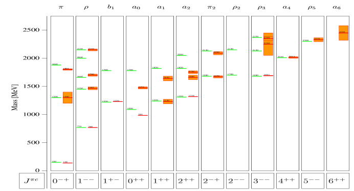
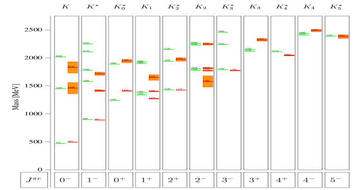
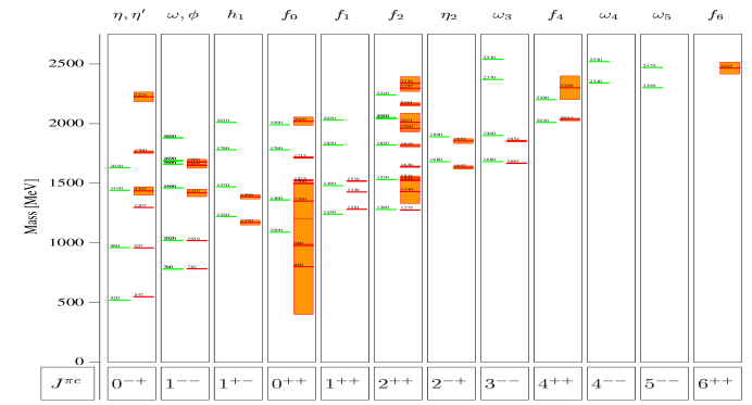
Figure 34: Mass spectra of light mesons for isovector (top),    isodoublet (center) and    isoscalar (bottom)    mesons. Experimental results (on the right, with error bars) are compared with the Godfrey–Isgur model (left) $\!{}^{{\bf?}}$.

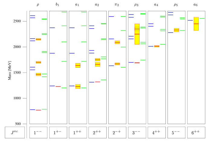
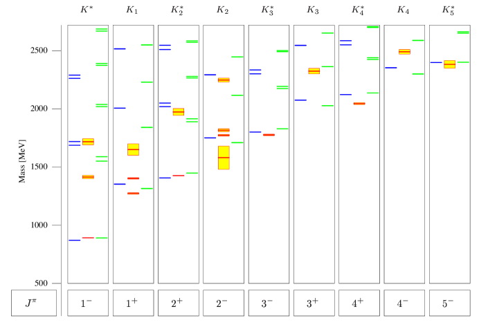
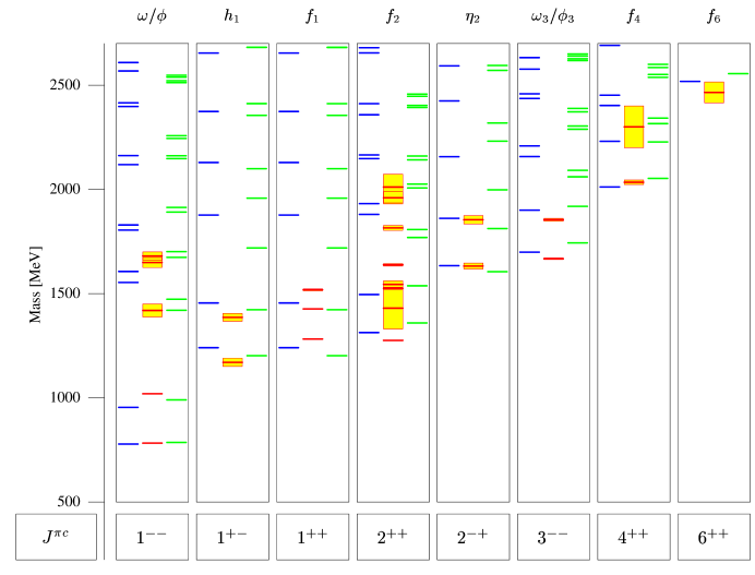
Figure 35: Mass spectra of light mesons for isovector (top), isodoublet (center) and isoscalar (bottom) mesons. Experimental results (for each partial wave in the center) are compared to the Bonn model, model A (left) and model B (right) $\!{}^{{\bf?}}$.

3.4 Quark models for baryons

The spatial wave function

The three-particle motion can be decomposed in Jacobian coordinates into two relative motions and the center-of-mass motion. The two internal oscillations can be assigned to an oscillation of two quarks in a diquark and of the third quark against the diquark. These two oscillators (usually called $\rho$– and $\lambda$ oscillators) support rotational and vibrational excitations and lead to a large number of expected resonances. The spatial wave functions of mesons can be classified in the 3-dimensional rotational group O(3); the three-body motion requires O(6).

The quark dynamics can be approximated by two harmonic oscillators. To first order, harmonic-oscillator wave-functions can be used. The rotational group O(6) can be expanded into O(6)$\rightarrow$O(3)$\otimes$O(2) $\!{}^{{\bf?}}$. Table 11 gives the expected multiplet structure in an O(6)$\otimes$SU(6) classification scheme for the four lowest excitation quantum numbers $N$. With increasing $N$, an increasing number of multiplets develop. The decomposition of the orbital wave-functions results in a complicated multiplet structure of harmonic-oscillator wave-functions. It should be mentioned that some of these multiplets need two quark excitations. In the lowest 20-plet, at $N=2$, two quarks are excited, each carrying one unit of orbital angular momentum; the two orbital angular momenta add to a total orbital angular momentum 1 with positive (!) parity.

Table 11: Multiplet-structure of harmonic oscillator wave functions $\!{}^{{\bf?}}$.

N	$\ O(6)$	$\ O(3)\otimes O(2)$	$\ (D,L^{P}_{N})$
0	1	$\ 1\otimes 1$	$\ (56,0^{+}_{0})$
1	6	$\ 3\otimes 2_{1}$	$\ (70,1^{-}_{1})$
2	20	$\ (5+1)\otimes 2_{2}$	$\ (70,2^{+}_{2})$, $\ (70,0^{+}_{2})$
		$\ 5\otimes 1$	$\ (56,2^{+}_{2})$
		$\ 3\otimes 1$	$\ (20,1^{+}_{2})$
	1	$\ 1\otimes 1$	$\ (56,0^{+}_{2})$
3	50	$\ (7+3)\otimes 2_{3}$	$\ (56,3^{-}_{3})$, $\ (20,3^{-}_{3})$, $\ (56,1^{-}_{3})$, $\ (20,1^{-}_{3})$
		$\ (7+5+3)\otimes 2_{1}$	$\ (70,3^{-}_{3})$, $\ (70,2^{-}_{3})$, $\ (70,1^{-}_{3})$
	6	$\ 3\otimes 2_{1}$	$\ (70,1^{-}_{3})$
4	105	$\ (9+5+1)\otimes 2_{4}$	$\ (70,4^{+}_{4})$, $\ (70,2^{+}_{4})$, $\ (70,0^{+}_{4})$
		$\ (9+7+5+3)\otimes 2_{2}$	$\ (70,4^{+}_{4})$, $\ (70,3^{+}_{4})$, $\ (70,2^{+}_{4})$, $\ (70,1^{+}_{4})$
		$\ (9+5+1)\otimes 1$	$\ (56,4^{+}_{4})$, $\ (56,2^{+}_{4})$, $\ (56,0^{+}_{4})$
		$\ (7+5)\otimes 1$	$\ (20,3^{+}_{4})$, $\ (20,2^{+}_{4})$
	20	$\ (5+1)\otimes 1$	$\ (70,2^{+}_{4})$, $\ (70,0^{+}_{4})$
		$\ 3\otimes 1$	$\ (20,1^{+}_{4})$
		$\ 5\otimes 1$	$\ (56,2^{+}_{4})$
	1	$\ 1\otimes 1$	$\ (56,0^{+}_{4})$

The ground state $N=0$ is readily identified with the well-known octet and decuplet baryons. The first excitation band ($N=1$) has internal orbital angular momentum L=1 ; both oscillators are excited coherently and there is one coherent excitation mode of the two oscillators. This information is comprised in the notation $3\otimes 2_{1}$. The next excitation band involves several dynamical realizations. The intrinsic orbital angular momentum L can be associated with two different quarks; the vector sum of the two l_i can be 0, 1 or 2, giving rise to the series $5\otimes 1$ to $1\otimes 1$ where the $3\otimes 1$ is antisymmetric w.r.t. quark exchange, and the other two are symmetric. Two linearly independent coherent two-oscillator excitations exist having mixed–symmetry spatial wave functions. The baryon is excited radially where the three quarks oscillate against their common center of mass. This mode is represented by $1\otimes 1$.

With increasing $N$ the number of multiplets increases strongly; multiplets belonging to bands of up to 12 were calculated $\!{}^{{\bf?}}$. So far, the multitude of predicted resonances have escaped experimental observation. This is the so–called missing-resonance problem and the basis for experimental searches for new states  $\!{}^{{\bf?},{\bf?}}$.

Quark model predictions

Figs. 37-37 show the mass spectra of N^∗ and $\Delta^{*}$ resonances using one–gluon exchange or instanton–induced interactions plus a linear confinement potential; the spectra for baryons with strangeness were also calculated in these models but are not reproduced here.

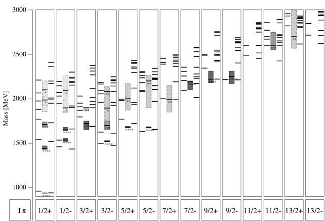
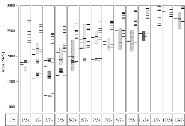
Figure 36: The spectrum of N^∗ resonances. For each partial wave, data (in the center row) are compared to predictions from one–gluon exchange $\!{}^{{\bf?}}$ (left) and from instanton–induced interactions $\!{}^{{\bf?}}$ (right).

Figure 37: The spectrum of $\Delta^{*}$ resonances. For each partial wave, data (in the center row) are compared to predictions from one–gluon exchange $\!{}^{{\bf?}}$ (left) and from instanton–induced interactions $\!{}^{{\bf?}}$ (right).

3.5 Conclusions

QCD inspired models are well suited to describe hadron mass spectra. In meson spectroscopy, wildly discrepant interpretations are found in the pseudoscalar and scalar sector. This is very exciting, since QCD allows not only the existence of $\bar{q}q$ mesons and $qqq$ baryons but also other forms of hadronic matter, like glueballs, hybrids, and multiquark states. In baryon physics, the most exciting issue is the possible discovery of the $\Theta^{+}(1540)$. If confirmed, the $\Theta^{+}(1540)$ would open a new spectroscopy, and it is still completely open what we will learn from it about QCD. Even if the $\Theta^{+}(1540)$ should not survive, I am convinced that baryon spectroscopy, due to the richness of the 3–particle dynamics, is the best testing ground to determine the degrees of freedom relevant to understand low–energy QCD. These questions will be discussed in the second half of the lecture series.

4 The quest for glueballs

4.1 Glueballs in “gluon-rich” processes

Glueballs, bound states of gluons with no constituent quarks, are predicted to exist and have been searched for in numerous experiments. There is an extensive folklore on how to hunt for glueballs $\!{}^{{\bf?}}$ and which distinctive features should identify them as non–$\bar{q}q$ mesons. Glueballs should, e.g., be produced preferentially in so–called gluon–rich processes; some are depicted in Fig. 38.

Figure 38: Diagrams possibly leading to the formation of glueballs: radiative J/$\psi$ decays, Pomeron-Pomeron collisions in hadron hadron diffractive scattering, and in $\rm p\bar{p}$ annihilation.

The most suggestive process is the radiative J/$\psi$ decay. The J/$\psi$ is narrow; the $D\bar{D}$ threshold is above the mass of the J/$\psi$ and the OZI rule suppresses decays of the $c\bar{c}$ system into light quarks. In most decays, the J/$\psi$ undergoes a transition into 3 gluons which then convert into hadrons. But the J/$\Psi$ can also decay into 2 gluons and a photon. The photon can be detected, the two gluons interact and must form glueballs - if they exist.

Central production is another process in which glueballs should be produced abundantly. In central production two hadrons pass by each other ‘nearly untouched’ and are scattered diffractively in forward direction. No valence quarks are exchanged. The process is often called Pomeron-Pomeron scattering. The absence of valence quarks in the production process makes central production a good place to search for glueballs.

In $\bar{p}p$ annihilation, quark-antiquark pairs annihilate into gluons, they interact and may form glueballs. Glueballs decay into hadrons and hence hadro–production of glueballs is always possible.

Production of glueballs should be suppressed in $\gamma\gamma$ collisions since photons couple to the intrinsic charges. So we should expect a glueball to be strongly produced in radiative J/$\psi$ decays but not in $\gamma\gamma$ fusion. Radial excitations might be visible only weakly in J/$\psi$ decays but they should couple to $\gamma\gamma$.

Further distinctive features can be derived from their decays (glueballs are flavor singlets). Decays to $\eta\eta^{\prime}$ identify a flavor octet; radiative decays of glueballs are forbidden. All these arguments have to be taken with a grain of salt: mixing of a glueball with mesons having the same quantum numbers can occur and would dilute any selection rule.

4.2 E/$\iota$ saga

The $\eta(1440)$ was the first glueball candidate and is still topic of a controversial discussion. It is instructive to outline its history.

Short history of the $\eta(1440)$

The E/$\iota$ was discovered 1967 in $p\bar{p}$ annihilation at rest into $(K\bar{K}\pi)\pi^{+}\pi^{-}$. It was the first meson found in a European experiment, and was called E-meson $\!{}^{{\bf?}}$. Mass and width were determined to $M=1425\pm 7,\Gamma=80\pm 10$  MeV; the quantum numbers to $J^{PC}=0^{-+}$. Also seen, 1967, was a state with $M=1420\pm 20,\Gamma=60\pm 20$ MeV but $J^{PC}=1^{++}$, now in the charge exchange reaction $\pi^{-}p\to n\rm K\bar{K}\pi$ using a 1.5 to 4.2 GeV/c pion beam $\!{}^{{\bf?}}$. Even though the quantum numbers had changed, it was still called E-meson.

In 1979, there was a claim for a $\eta(1295)$ which was later confirmed in several experiments $\!{}^{{\bf?}}$. The E–meson was observed in 1980 in radiative J/$\psi$ decays $\!{}^{{\bf?}}$ into $(K\bar{K}\pi)$ with $M=1440\pm 20,\Gamma=50\pm 30$ MeV; and quantum numbers ‘rediscovered’ $\!{}^{{\bf?}}$ to be $J^{PC}=0^{-+}$. It was now called $\iota(1440)$ to underline the claim that it was the $\iota^{\rm st}$ glueball. The $\iota(1440)$ is a very strong signal, one of the strongest in radiative J/$\psi$ decays (see Fig. 39). The radial excitation $\eta(1295)$ is not seen in this reaction; hence the $\iota(1440)$ must have a different nature. At that time it was proposed (and often still is) to be a glueball.

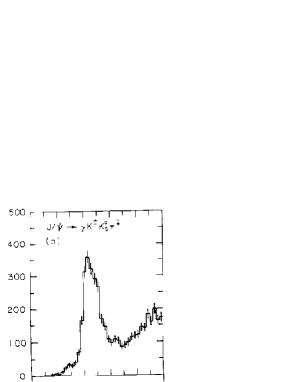
1295 MeV $\bf\Uparrow$    $\bf\Uparrow$  1440 MeV

Further studies showed that the $\iota(1440)$ is split into two components, a $\eta_{L}\to a_{0}(980)\pi$ with $M=1405\pm 5,\Gamma=56\pm 6$ MeV and a $\eta_{H}\to\rm K^{*}\bar{K}+\bar{K}^{*}K$ with $M=1475\pm 5,\Gamma=81\pm 11$ MeV. Hence, there seem to be 3 $\eta$ states in the mass range from 1280 to 1480  MeV.

Figure 39: The $\iota(1440)$ is a strong signal in radiative J/$\psi$ decay. It cannot be described by a single Breit-Wigner resonance. There is no evidence for the $\eta(1295)$ from radiative J/$\psi$ decay $\!{}^{{\bf?}}$.

The $\eta(1295)$ is then likely the radial excitation of the $\eta$. It is mass degenerate with the $\pi(1300)$, hence the pseudoscalar radial excitations seem to be ideally mixed ! Then, the $\bar{s}s$ partner is expected to have a mass 240 MeV higher. The $\eta_{H}$ could play this role. The $\eta_{L}$ finds no slot in the spectrum of $\bar{q}q$ mesons; the low mass part of the $\iota(1440)$ could be a glueball. This conjecture is consistent with the observed decays. A pure flavor octet $\eta(xxx)$ state decays into $\rm K^{*}K$ but not into $a_{0}(980)\pi$. In turn, a pure flavor singlet $\eta(xxx)$ state decays into $a_{0}(980)\pi$ but not into $\rm K^{*}K$. (Both, $(\bar{u}u+\bar{d}d)$ and $\bar{s}s$ states, may decay into $\rm K^{*}K$ and $a_{0}(980)\pi$. For $\sigma\eta$ decays there are no flavor restrictions.) The $\eta_{H}$, with a large coupling to $\rm K^{*}K$, cannot possibly be a glueball, while the $\eta_{L}$ with its $a_{0}(980)\pi$ decay mode can be.

Two quantitative tests have been proposed to test if a particular meson is glueball–like: the stickiness and the gluiness. The stickiness of a resonance R with mass $m_{\rm R}$ and two–photon width $\Gamma_{{\rm R}\mbox{$\rightarrow$}\gamma\gamma}$ is defined as:

$$S_{\rm R}=N_{l}\left(\frac{m_{\rm R}}{K_{{\rm J}\to\gamma{\rm R}}}\right)^{2l+1}\frac{\Gamma_{{\rm J}\to\gamma{\rm R}}}{\Gamma_{{\rm R}\mbox{$\rightarrow$}\gamma\gamma}}\ ,$$

where $K_{{\rm J}\to\gamma{\rm R}}$ is the energy of the photon in the J rest frame, $l$ is the orbital angular momentum of the two initial photons or gluons ($l=1$ for $0^{-}$), $\Gamma_{{\rm J}\to\gamma{\rm R}}$ is the J radiative decay width for R, and $N_{l}$ is a normalization factor chosen to give $S_{\eta}=1$. The L3 collaboration determined $\!{}^{{\bf?}}$ this parameter to $S_{\eta(1440)}=79\pm 26$.

The gluiness ($G$) was introduced $\!{}^{{\bf?},{\bf?}}$ to quantify the ratio of the two–gluon and two–photon coupling of a particle, it is defined as:

$$G=\frac{9\,e^{4}_{q}}{2}\,\biggl{(}\frac{\alpha}{\alpha_{s}}\biggr{)}^{2}\,\frac{\Gamma_{{\rm R}\mbox{$\rightarrow$}{\rm gg}}}{\Gamma_{{\rm R}\mbox{$\rightarrow$}\gamma\gamma}}\ ,$$

where $e_{q}$ is the relevant quark charge, calculated assuming equal amplitudes for $\mbox{u}\bar{\mbox{u}}$ and $\mbox{d}\bar{\mbox{d}}$ and zero amplitude for $\mbox{s}\bar{\mbox{s}}$. $\Gamma_{{\rm R}\mbox{$\rightarrow$}{\rm gg}}$ is the two–gluon width of the resonance R, calculated from equation (3.4) of Reference $\!{}^{{\bf?}}$. Whereas stickiness is a relative measure, the gluiness is a normalised quantity and is expected to be near unity for a $\mbox{q}\bar{\mbox{q}}$ meson. The L3 collaboration determined $\!{}^{{\bf?}}$ this quantity to $G_{\eta(1440)}=41\pm 14$.

These numbers can be compared to those for the $\eta^{\prime}$ for which $S_{\eta^{\prime}}=3.6\pm 0.3$ and $G_{\eta^{\prime}}=5.2\pm 0.8$ for $\alpha_{s}(958MeV)=0.56\pm 0.07$ is determined. Hence also the $\eta^{\prime}$ is ‘gluish’, but much more the $\eta_{L}$. The $\eta_{L}$ is the first glueball !

We should not stop here, instead we should also collect arguments which speak against this interpretation. Is the $\eta_{H}$ a $\bar{s}s$ state, and is the $\eta(1295)$ the radial excitation of the $\eta$ ?

As $\bar{s}s$ state, the $\eta_{H}$ should be produced in $\rm K^{-}\ p\to\ \Lambda\ \ \eta_{H}$.

As $\bar{s}s$ state, the $\eta_{H}$ should not be produced in $\rm\pi^{-}\ p\to\ n\ \eta_{H}$.

It is not !

But it is !

In the diagram, the thicker lines represent a strange quarks. The $\eta(1440)$ region does not contain a large $s\bar{s}$ component. The $\eta_{H}=\eta_{s\bar{s}}$ is not a $s\bar{s}$ state !

Fig. 39, with the strong $\eta(1440)$ signal, shows no sign of the hypothetical radial excitation of the $\eta$, of the $\eta(1295)$. Is there evidence for this state in other reactions ?

The $\eta(1295)$ and the $\eta(1440)$ in $\gamma\gamma$ at LEP

Photons couple to charges; in $\gamma\gamma$ fusion a radial excitation is hence expected to be produced more frequently than a glueball. In $\gamma\gamma$ fusion, both electron and positron scatter by emitting a photon. If the momentum transfer to the photons is small, the $e^{+}$ and $e^{-}$ are scattered into forward angles (passing undetected through the beam pipe), thus

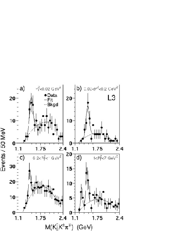
$\gamma\gamma\to\eta(1295)$:

CG${(1,0)+(1,0)\to(0,0)}\neq 0$

$\gamma\gamma\not\to f_{1}(1285)$:

CG${}_{(1,0)+(1,0)\to(1,0)}=0$

$\gamma^{*}\gamma\to f_{1}(1285)$:

CG$\_{(1,M)+(1,0)\to(1,M)}\neq 0$

Figure 40: $\rm\gamma\gamma^{*}\to K^{0}_{s}K^{\pm}\pi^{\mp}$ from L3. At low $q^{2}$, a peak at 1440 MeV is seen, it requires high $q^{2}$ to produce a peak at 1285 MeV. A pseudoscalar state is produced also at vanishing $q^{2}$ while $J^{PC}=1^{++}$ is forbidden for $q^{2}\to 0$. Hence the structure at 1285 MeV is due to the $f_{1}(1285)$ and not due to $\eta(1295)$. There is no evidence for the $\eta(1295)$ from $\gamma\gamma$ fusion. The stronger peak contains contributions from the $\eta(1440)$ and $f_{1}(1420)$ $\!{}^{{\bf?}}$.

the two photons are nearly real. If the $e^{+}$ or $e^{-}$ has a large momentum transfer, the photon acquires mass, and we call the process $\gamma\gamma^{*}$ collision.

Fig. 40 shows data from the L3 experiment $\!{}^{{\bf?}}$. Selection rules for production of $\eta$ and $f_{1}$ mesons are also given. The peak at low mass and high $Q^{2}$ must be the $f_{1}(1285)$, since it is not produced for low $Q^{2}$. The higher mass peak can have contributions from both, from the $f_{1}(1420)$ and the $\eta(1440)$. These contributions can be separated due to their different dependence on $Q^{2}$ or $P_{T}^{2}$. As a result we can state that the $\eta(1440)$ is definitely produced in $\gamma\gamma$ collisions. There is no sign of the $\eta$(1295). The coupling of the $\eta$(1440) to photons is stronger than that of the $\eta$(1295): the assumption that the $\eta$(1295) is a $(u\bar{u}+d\bar{d})$ radial excitation must be wrong ! The mass of the pseudoscalar resonance in $\gamma\gamma$ fusion is about 1460 MeV, and it decays mainly into $\rm K^{*}K$. Hence we identify the state with the $\eta_{H}$.

The $\eta(1295)$ and $\eta(1440)$ in $p\bar{p}$ annihilation

The $\eta(1295)$ and $\eta(1440)$ can be searched for in the reaction $p\bar{p}\to\pi^{+}\pi^{-}\eta(xxx)$, $\eta(xxx)\to\eta\pi^{+}\pi^{-}$. The search is done by assuming the presence of a pseudoscalar state of given mass and width, mass and width are varied and the likelihood of the fit is plotted. Fig. 41 shows such a plot $\!{}^{{\bf?}}$. A clear pseudoscalar resonance signal is seen at 1405 MeV. Two decay modes are observed, $a_{0}(980)\pi$ and $\eta\sigma$ with a ratio $0.6\pm 0.1$.

A scan for an additional $0^{+}0^{-+}$ resonance provides no evidence for the $\eta(1295)$ but for a second resonance at 1480 MeV, see Fig. 41, with $M=1490\pm 15,\Gamma=74\pm 10$. This is the $\eta_{H}$. It decays to $a_{0}(980)\pi$ and $\eta\sigma$ with a ratio $0.16\pm 0.10$.

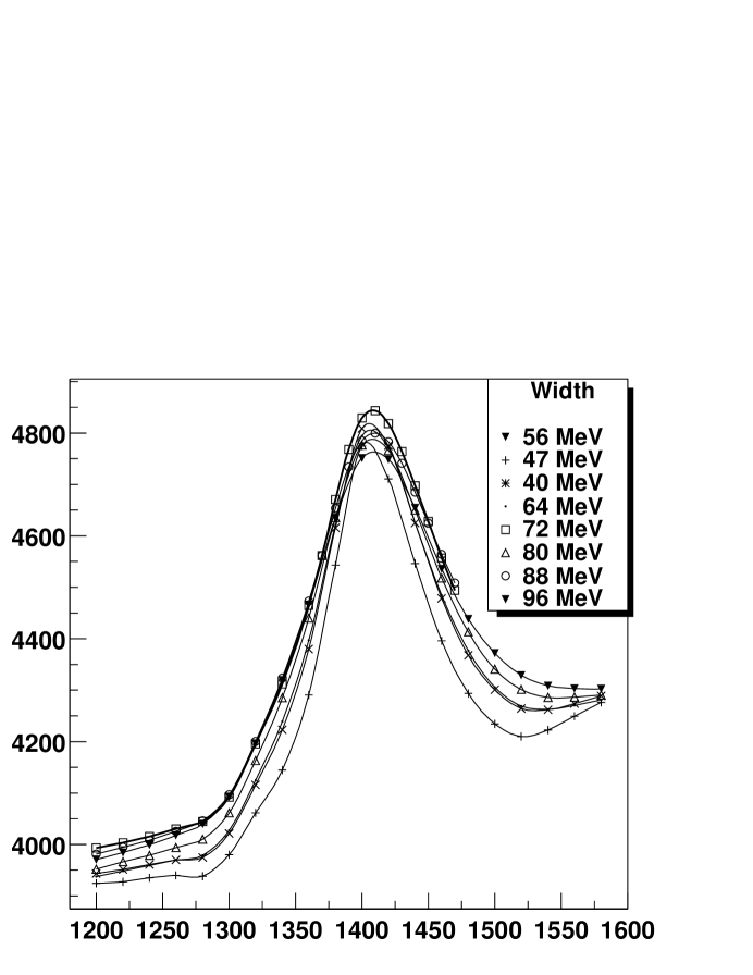
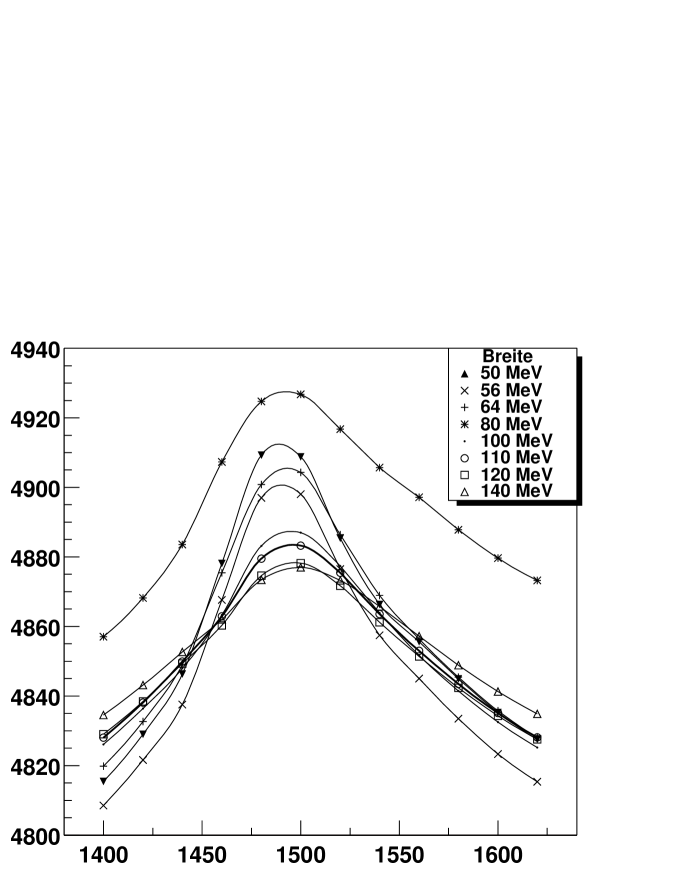
Figure 41: Scan for a $0^{+}0^{-+}$ resonance with different widths. The likelihood optimizes for $M=1407\pm 5,\Gamma=57\pm 9$ MeV. The resonance is identified with the $\eta_{L}$. A search for a second pseudoscalar resonance (right panel) gives evidence for the $\eta_{H}$ with $M=1490\pm 15,\Gamma=74\pm 10$ MeV. From $\!{}^{{\bf?}}$.

$E/\iota$ decays in the ${}^{3}P_{0}$ model

The phenomena observed in the pseudoscalar sector are confusing: The $\eta(1295)$, the assumed radial excitation of the $\eta$, is only seen in $\pi^{-}p\to n(\eta\pi\pi)$, not in $p\bar{p}$ annihilation, nor in radiative J/$\psi$ decay, nor in $\gamma\gamma$ fusion. In all these reactions, except perhaps in radiative J/$\psi$ decays, it should have been observed. There is no reason for it not being produced if it is a $\bar{q}q$ state. On the other hand, we do not expect glueballs, hybrids or multiquark states so low in mass. In the 70’s, the properties of the $a_{1}(1260)$ were obscured by the so–called Deck effect ($\rho$–$\pi$ rescattering in the final state). Possibly, $a_{0}(980)\pi$ rescattering fakes a resonant–like behavior but the $\eta(1295)$ is too narrow to make this possibility realistic. Of course, there is the possibility that the $\eta(1295)$ is mimicked by feed–through from the $f_{1}(1285)$. In any case, we exclude the $\eta(1295)$ from the further discussion.

The next puzzling state is the $\eta(1440)$. It is not produced as $\bar{s}s$ state but decays with a large fraction into $\rm K\bar{K}\pi$ and it is split into two components. We suggest that the origin of all these anomalies are due to a node in the wave function of the $\eta(1440)$ ! The node has an impact on the decay matrix element which were calculated by $\!{}^{{\bf?}}$ within the ${}^{3}P_{0}$ model.

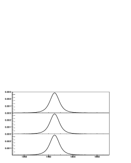
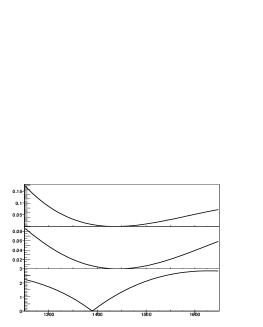
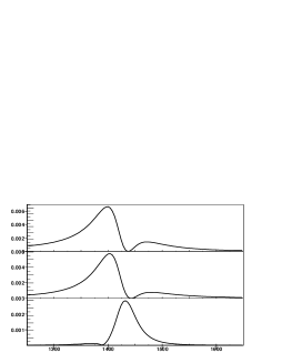
Figure 42: Amplitudes for $\eta(1440)$ decays to $a_{0}\pi$ (first row), $\sigma\eta$ (second row): $\rm K^{*}\bar{K}$ (third row) the Breit-Wigner functions are shown on the left, then the squared decay amplitudes $\!{}^{{\bf?}}$ and, on the right, the resulting squared transition matrix element.

The matrix elements for decays of the $\eta(1440)$ as a radial excitation (=$\eta_{R}$) depend on spins, parities and decay momenta of the final state mesons. For $\eta_{R}$ decays to $\rm K^{*}K$, the matrix element is given by

$$f_{P}=\frac{2^{9/2}\cdot 5}{3^{9/2}}\cdot x\left(1-\frac{2}{15}x^{2}\right).$$

In this expression, $x$ is the decay momentum in units of 400 MeV/c, the scale is determined from comparisons of measured partial widths to model predictions. The matrix element vanishes for $x=0$ and $x^{2}=15/2$, or $p=1$ GeV/c. These zeros have little effect on the shape of the resonance.

The matrix element for $\eta_{R}$ decays to $a_{0}(980)\pi$ or $\sigma\eta$ has the form

$$f_{S}=\frac{2^{4}}{3^{4}}\cdot\left(1-\frac{7}{9}x^{2}+\frac{2}{27}x^{2}\right)$$

and vanishes for $p=0.45$ GeV/c. So, if $\eta_{R}=\eta(1440)$, the decay to $a_{0}(980)\pi$ vanishes at the mass 1440 MeV. This does have a decisive impact on the shape, as seen in Figure 42. Shown are the transition matrix elements as given by Barnes et al. $\!{}^{{\bf?}}$ and the product of the squared matrix elements and a Breit–Wigner distribution with mass 1420 MeV and a width of 60 MeV.

We note that $\eta(1440)\to a_{0}(980)\pi$ and $\to\rm K^{*}K$ have different peak positions; at approximately the $\eta_{L}$ and $\eta_{H}$ masses. Hence there is no need to introduce the $\eta_{L}$ and $\eta_{H}$ as two independent states. One $\eta(1420)$ and the assumption that it is a radial excitation describes the data.

This can be further tested by following the phase motion of the $a_{0}(980)\pi$ or $\sigma\eta$ isobar $\!{}^{{\bf?}}$. The phase changes by $\pi$ and not by 2$\pi$, see Fig. 43.

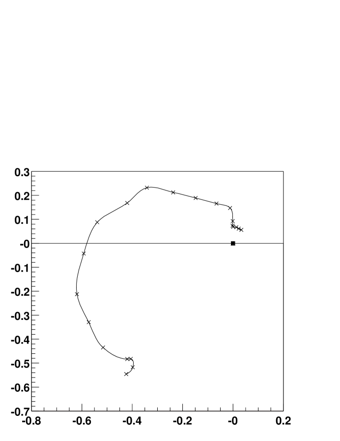
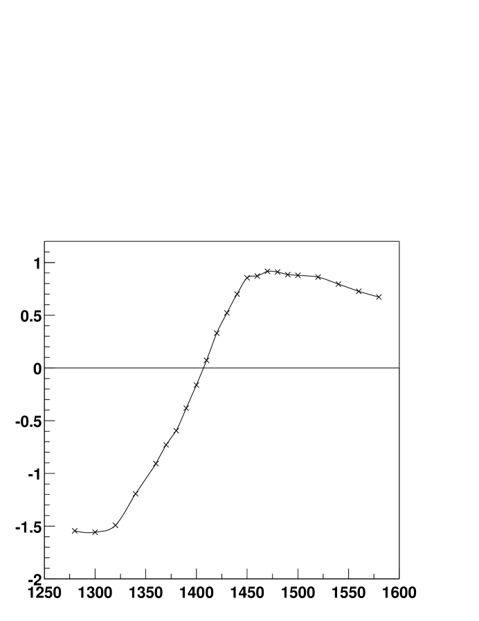
Figure 43: Complex amplitude and phase motion of the $a_{0}(980)\pi$ isobars in $\rm p\bar{p}$ annihilation into $4\pi\eta$. In the mass range from 1300 to 1500 MeV the phase varies by $\pi$ indicating that there is only one resonance in the mass interval. The $\sigma\eta$ (not shown) exhibits the same behavior $\!{}^{{\bf?}}$.

Conclusions

We summarize the results for the radial excitations of pseudoscalar mesons.

1. The $\eta(1295)$ is not a $q\bar{q}$ meson.

2. The $\eta(1440)$ wave function has a node leading to two appearantly different states $\eta_{L}$ and $\eta_{H}$.

3. The node suppresses OZI allowed decays into $a_{0}(980)\pi$ and allows $K^{*}K$ decays.

4. There is only one $\eta$ state, the $\eta(1420)$ in the mass range from 1200 to 1500 MeV and not 3 !

5. The $\eta(1440)$ is the radial excitation of the $\eta$.

6. The radial excitation of the $\eta^{\prime}$ is expected at about 1800 MeV; it might be the $\eta(1760)$.

The following states are most likely the pseudoscalar ground states and radial excitations:

$1^{1}S_{0}$	$\pi$	$\eta^{\prime}$	$\eta$	K
$2^{1}S_{0}$	$\pi(1300)$	$\eta(1760)$	$\eta(1440)$	K(1460)

Warning lesson from the $\bf\iota(1440)$:

You can build up a case, convince the community, yet still be wrong !

4.3 Glueball masses from the lattice

At the time when the $\eta(1440)$ was claimed to be the first glueball, mass estimates were not yet reliable and required normalization. Often, the mass of the $\eta(1440)$ was used as input to define the scale of glueball masses. Today, the best estimates come from lattice gauge calculations. In figure 44, we show the results obtained from an anisotropic lattice (where the (Eukledian) time grid extends over more grid points than the spatial grid).

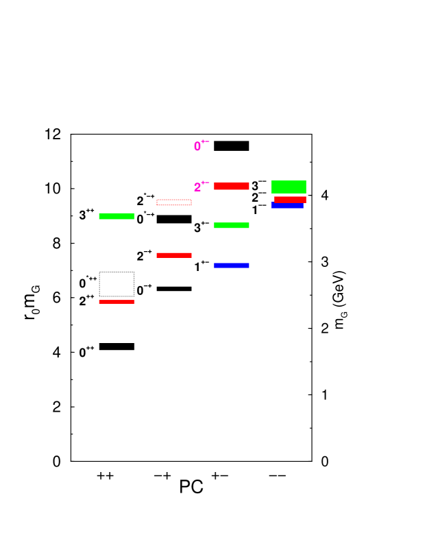
Figure 44: The glueball spectrum from an anisotropic lattice study $\!{}^{{\bf?}}$. A pseudoscalar glueball should have a mass of about 2.5 GeV ! Obviously, the $\eta(1440)$ cannot be a glueball. The scalar glueball is expected at $1.7$ GeV.

4.4 The enigmatic scalar mesons

The lowest–mass glueball has scalar quantum numbers. Its predicted mass ($\sim 1700$ MeV) falls into a region in which one may hope to get a consistent picture of the mass spectrum of all scalar mesons. Table 12 lists the spectrum of scalar mesons as given by the Particle Data Group. Let us recall what we expect: scalar mesons have intrinsic orbital angular momentum $L=1$ and quark spin $S=1$ which couple to $J=0$. Since spin–orbit interactions are not very large (the $a_{1}(1260)$ and $a_{2}(1320)$ masses are not very different), we might expect an $a_{0}(1300)$, a K${}^{*}_{0}(1430)$, and two $f_{0}$ with a mass difference of about 250 MeV (like the $f_{2}(1270)$ and $f_{2}(1525)$ mass splitting) or about 400 MeV which is the mass difference between the $\eta$ and the $\eta^{\prime}$. In the case of baryons, we have seen that radial excitations have a gap in mass square to the ground states in the order of 1.2 GeV². Thus we expect radial excitations to have masses of about 1700 MeV and above. Including radial excitations, there should be two $a_{0}$, two K${}^{*}_{0}$ (which we find) and four $f_{0}$’s. But there are 7 $f_{0}$’s. (At high masses we combine separate candidates in one entry. We will omit the $f_{0}(2200,2330)$ from our discussion.) Hence we need to identify the four $\bar{q}q$ states and discuss what the nature of the remaining states might be.

I = 1/2	I = 1	I = 0
		$f_{0}(600)$
	$a_{0}(980)$	$f_{0}(980)$
		$f_{0}(1370)$
$K_{0}^{*}(1430)$	$a_{0}(1490)$	$f_{0}(1500)$
		$f_{0}(1710)$
$K_{0}^{*}(1950)$
		$f_{0}(2020,2100)$
		$f_{0}(2200,2330)$

Table 12: The Particle Data Group lists 12 scalar mesons. Within the quark model we expect 4 ground state mesons and 4 radial excitations.

Scalar mesons below 1 GeV

The $f_{0}(600)$, the lowest mass scalar meson often called $\sigma(600)$, has rather ill-defined properties. The Particle Data Group assigns to it a mass range from 400 to 1200 MeV. In partial wave analyses, it is seen as a pole at about 470 MeV. However, the phase reaches $90^{\circ}$ only at $\sim 780$ MeV. Its nature is hotly debated: a very attractive conjecture assigns the $\sigma(600)$ to a nonet ($a_{0}(980),\sigma(600),f_{0}(980)$, $\kappa(900)$) where $\kappa(900)$ represents the K$\pi$ S–wave which may have a pole at about 900 MeV. As a nonet of ‘normal’ $q\bar{q}$ mesons, their mass seem to be too low, but Jaffe $\!{}^{{\bf?}}$ showed that the nonet may be composed of $qq\bar{q}\bar{q}$ states where the $a_{0}(980)$ and $f_{0}(980)$ carry an additional $s\bar{s}$ pair (explaining their large coupling to $\rm K\bar{K}$). Or, they may be relativistic S-wave $q\bar{q}$ states (‘chiralon’)s $\!{}^{{\bf?}}$. In the limit of chiral symmetry, we expect scalar partners of the pseudoscalar nonet, and these 9 scalar resonances are identified as scalar companions of the pseudoscalar mesons.

Even if all four particles ($\sigma(600),\kappa(900),a_{0}(980)$ and $f_{0}(980)$ exist, there is no proof that they form one nonet $\!{}^{{\bf?}}$. Other scenarios are feasible where the dynamical origin of the $\sigma(600),\kappa(900)$ and of the $a_{0}(980)$ and $f_{0}(980)$ are different. The $a_{0}(980)$ and $f_{0}(980)$ are often considered as $\rm K\bar{K}$ molecular–like bound states. Their masses are close to the $\rm\bar{K}K$ threshold, hence K and $\rm\bar{K}$ could be weakly bound, forming two resonances in isospin $I=0$ and $I=1$, as suggested by Isgur and Weinstein $\!{}^{{\bf?}}$, by Speth and collaborators $\!{}^{{\bf?}}$ or by Markushin and Locher $\!{}^{{\bf?}}$. The $\sigma(600)$ and $\kappa(900)$ are both very wide objects; they might be due to attractive $\pi\pi$ or $\rm K\pi$ interactions, generated dynamically, (or by ‘left–hand cuts’ in a technical language). Practically, the $\sigma(600)$ and $\kappa(900)$ do not play a role in the discussion of glueballs, and the reader is referred to a recent review $\!{}^{{\bf?}}$.

Scalar mesons above 1 GeV

The Crystal Barrel collaboration proposed the existence of two scalar isoscalar mesons, the $f_{0}(1370)$ and $f_{0}(1500)$. Their main properties were derived from four Dalitz plots  $\!{}^{{\bf?},{\bf?},{\bf?},{\bf?}}$, shown in figure 45, and from the analysis of different 5 pion final states $\!{}^{{\bf?},{\bf?},{\bf?},{\bf?}}$. In the 3$\pi^{0}$ (upper left) and the $\pi^{0}$2$\eta$ (upper right) Dalitz plots the $f_{0}(1500)$ is clearly seen as band structure. In $\pi^{0}$$\eta$$\eta^{\prime}$ a strong threshold enhancement in the $\eta$$\eta^{\prime}$ invariant mass is seen (lower left); the final state K_lK_l$\pi^{0}$ has prominent K^∗ bands; their interference with the $f_{0}(1500)$ makes the intensity so large in the left corner of the Dalitz plot (lower right). The reactions $p\bar{p}\to\pi^{+}\pi^{-}3\pi^{0}$ $\!{}^{{\bf?}}$, $p\bar{p}\to 5\pi^{0}$ $\!{}^{{\bf?}}$, $p\bar{n}\to\pi^{-}4\pi^{0}$  $\!{}^{{\bf?}}$ and $p\bar{n}\to 2\pi^{-}2\pi^{0}\pi^{+}$  $\!{}^{{\bf?}}$ were studied to determine decays into 4 pions.

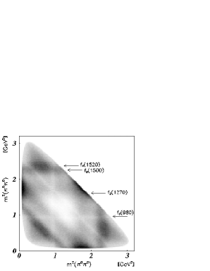
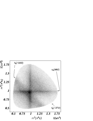
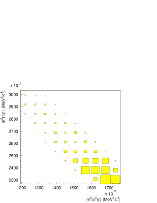
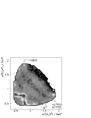
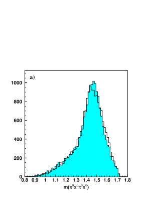
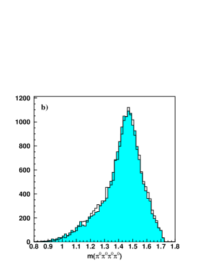
Figure 45: Dalitz plots for $p\bar{p}$ annihilation at rest into 3$\pi^{0}$ (upper left), $\pi^{0}2\eta$ (upper right), $\pi^{0}\eta\eta^{\prime}$ (lower left), $\rm K_{l}K_{l}\pi^{0}$ (lower right). The $f_{0}(1370)$ contributes to (a,b,d), the $f_{0}(1500)$ to all 4 reactions. The $\rm K_{l}K_{l}\pi^{0}$ is difficult to interpret in the black-and-white version; the colored Dalitz plot can be found on the web. The data are from $\!{}^{{\bf?},{\bf?},{\bf?},{\bf?}}$. The two lowest plots show the 4$\pi^{0}$ invariant mass in the reaction $\rm\bar{p}n\to\pi^{-}4\pi^{0}$. A fit (including other amplitudes) with one scalar state fails; two scalar resonances at 1370 and 1500 MeV give a good fit. Note that the full 8-dimensional phase space is fitted and not just the mass projection shown here $\!{}^{{\bf?}}$.

We have seen that decays of mesons are constrained by SU(3) relations. So there is hope that the glueball nature of a state can be unraveled by inspecting the coupling to various final states.

Table 13 lists partial widths of the $f_{0}(1370)$ and $f_{0}(1500)$ as derived from the Crystal Barrel Collaboration. Neither the $f_{0}(1370)$ nor the $f_{0}(1500)$, has a large coupling to $\rm K\bar{K}$, so none of them carries a large $s\bar{s}$ fraction. For an interpretation as ground state plus radial excitation, their mass difference is too small. Hence one of them might be the scalar glueball. The partial decay widths for the decays into $\eta$$\eta$ and $\eta$$\eta^{\prime}$ and the smallness of the $\rm K\bar{K}$ coupling of the $f_{0}(1500)$ show that the $f_{0}(1500)$ cannot be a pure glueball: For a glueball or any other isosinglet meson we expect ratios for $\pi\pi$ : $\eta$$\eta$ : $\eta$$\eta^{\prime}$ : $\rm K\bar{K}$ of 3 :1 : 0 : 4, after removal of phase space. Since the coupling to $\eta$$\eta^{\prime}$ is large, the $f_{0}(1500)$

Table 13: Partial decay widths of the $f_{0}(1370)$ $f_{0}(1370)$rrr $f_{0}(1370)$ and $f_{0}(1500)$.

	$f_{0}(1370)$	$f_{0}(1500)$
$\Gamma_{tot}$	$\sim 350$	$\sim 109$
$\Gamma_{\pi\pi}$	$\sim 90$	$\sim 32$
$\Gamma_{\eta\eta}$	$\sim 1$	$\sim 6$
$\Gamma_{\eta\eta^{\prime}}$		$\sim 3$
$\Gamma_{\bar{K}K}$	$\sim 50$	$\sim 6$
$\Gamma_{4\pi}$	$\sim 210$	$\sim 62$
$\Gamma_{\sigma\sigma}$	$\sim 106$	$\sim 20$
$\Gamma_{\rho\rho}$	$\sim 55$	$\sim 10$
$\Gamma_{\pi^{*}\pi}$	$\sim 36$	$\sim 25$
$\Gamma_{a_{1}\pi}$	$\sim 13$	$\sim 7$

cannot be a pure glueball, it must mix with nearby states. The $f_{0}(1370)$ has important couplings to two pairs of $\pi^{0}$-mesons, to $\sigma\sigma$. This is evident from the two plots at the bottom of figure 45.

Three striking peaks were observed in the $\eta$$\eta$ invariant mass spectrum produced in $\bar{p}p$ annihilation in flight into $\pi^{0}$$\eta$$\eta$ $\!{}^{{\bf?}}$, $1500,1750$ and $2100$ MeV. The data were not decomposed into partial waves in a partial wave analysis, so the peaks could have J${}^{\rm P\rm C}=0^{++}$, $2^{++}$, or higher. If the states would have J${}^{\rm P\rm C}=2^{++}$, their decay into $\eta$$\eta$ would be suppressed by the angular momentum barrier. The peaks are seen very clearly suggesting $0^{++}$ quantum numbers.

The same pattern of states was seen at BES in radiative J/$\psi$ decays $\!{}^{{\bf?}}$ into 2$\pi^{+}$2$\pi^{-}$. The results of a partial wave analysis in figure 46 show a slowly rising instrumental background and 3 important contributions with scalar, pseudoscalar and tensor quantum numbers.

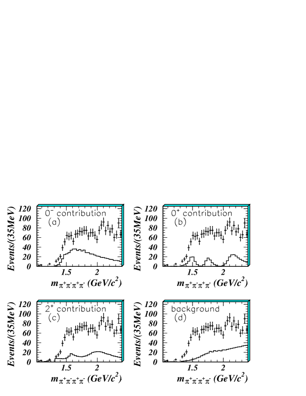
Figure 46: Partial wave decomposition of radiative J/$\psi$ decays into 2$\pi^{+}$2$\pi^{-}$$\!{}^{{\bf?}}$.

The scalar part contains three resonances, at 1500, 1710 and 2100 MeV. This pattern of states was already suggested in a reanalysis of MARKIII data $\!{}^{{\bf?}}$. The $f_{0}(1500),f_{0}(1710)$ and the $f_{0}(2100)$ have a similar production and decay pattern. Neither a $f_{0}(1370)$ nor a ‘background’ intensity is assigned to the scalar isoscalar partial wave.

4.5 Scalar mesons: interpretation

There is no agreement how to interpret the scalar spectrum, there are numerous experimental and theoretical contributions to this field. Here we discuss three typical scenarios.

The ‘narrow’ glueball

The first interpretation $\!{}^{{\bf?}}$, also adopted by the Particle Data Group, identifies the $a_{0}(980)$ and $f_{0}(980)$ as non–$q\bar{q}$ states. They might form, together with the $\sigma(600)$ and $\kappa(900)$, a nonet of four–quark states, or they could form a nonet of ‘chiralons’, but they are left out for further discussion. In the mass region where the scalar $1^{3}P_{0}$ mesons are expected, there are now 10 states while the quark model predicts only 9 (3 $a_{0}1450)$, 4K${}^{*}_{0}(1430)$, and 2 $f_{0}$’s). One of the states, $f_{0}(1370)$ or $f_{0}(1500)$ or $f_{0}(1710)$, must be the scalar glueball !

However, the $f_{0}(1500)$ couples strongly to $\eta\eta^{\prime}$; these are two SU(3) orthogonal states and cannot come from a singlet. The $f_{0}(1500)$ must hence have a strong flavor–octet component, it cannot be a pure glueball. The $f_{0}(1370)$ and $f_{0}(1500)$ decay strongly to $2\pi$ and into $4\pi$ and weakly to $\rm\bar{K}K$, they both cannot carry a large $\bar{s}s$ component. The $f_{0}(1370)$ is, perhaps, too light to be the scalar glueball. So, none of the three states ’smells’ like a glueball. A way out is mixing; the two scalar $\bar{q}q$ states and the scalar glueball have the same quantum numbers, they mix and form the three observed states. Table 14 summarizes this interpretation.

Table 14: Possible interpretation of the scalar mesons. The three states $f_{0}(1370)$, $f_{0}(1500)$ and $f_{0}(1710)$ originate from 2 $q\bar{q}$ states and a glueball.

I = 1/2	I = 1	I = 0
		$f_{0}(600)$		$\sigma(600)$ meson
				chiral partner of the $\pi$
	$a_{0}(980)$	$f_{0}(980)$		$\rm K\bar{K}$ molecules
		$f_{0}(1370)$		$q\bar{q}$ state
$K_{0}^{*}(1430)$	$a_{0}(1490)$	$f_{0}(1500)$		2 $q\bar{q}$ states, glueball
		$f_{0}(1710)$		$q\bar{q}$ state
$K_{0}^{*}(1950)$				$q\bar{q}$ state
		$f_{0}(2100)$		$q\bar{q}$ state
		$f_{0}(2200,2330)$		$q\bar{q}$ state

Several mixing scenarios have been suggested $\!{}^{{\bf?},{\bf?},{\bf?},{\bf?},{\bf?},{\bf?},{\bf?}}$ and some of them are capable of reproducing the decay pattern. So, in these scenarios two scalar states plus an intruder, the scalar glueball, mix. The lattice gauge predictions for the existence of a glueball and the mass estimates are beautifully confirmed, and there is only the need to confirm some further glueball predictions.

The ‘narrow’ glueball scrutinized

An important ingredient of the ‘narrow–glueball’ is the interpretation of the $f_{0}(980)$ and $a_{0}(980)$ as alien objects, unrelated to the spectroscopy of $\mbox{q}\bar{\mbox{q}}$ mesons. Several experiments were directed to determine the structure of these two mesons, like two-photon production $\!{}^{{\bf?}}$, or $\Phi$ radiative decay rate into $f_{0}(980)$ $\!{}^{{\bf?},{\bf?}}$ and into $a_{0}(980)$ $\!{}^{{\bf?},{\bf?}}$. The conclusions drawn from these results are, however, ambiguous.

At LEP, the fragmentation of quark- and gluon jets has been studied intensively $\!{}^{{\bf?}}$. In particular the inclusive production of the $f_{0}(980)$ and $a_{0}(980)$ provides insight into their internal structure. Some total inclusive rates are listed in Table 15. The rates depend on the meson mass and on the spin multiplicity. The three mesons $\eta^{\prime}$, $f_{0}(980)$ and $a_{0}(980)$ - which have very similar masses - have production rates which are nearly identical (the two charge modes of the $a_{0}(980)^{\pm}$ need to be taken into account). Hence there is primary evidence that the three mesons have the same internal structure and that they are all three $q\bar{q}$ states. This conclusion was substantiated by further studies $\!{}^{{\bf?}}$ of the production characteristics of the $f_{0}(980)$ as compared to those of f${}_{2}(1270)$ and $\Phi(1020)$ mesons, and with the Lund string model of hadronization within which the $f_{0}(980)$ is treated as a conventional meson. No difference is observed in any of these comparisons between the $f_{0}(980)$ and the f${}_{2}(1270)$ and $\Phi(1020)$.

$\pi^{0}$	$9.55\pm 0.06\pm 0.75$
$\eta$	$0.97\pm 0.03\pm 0.11$
$\eta^{\prime}$	$0.14\pm 0.01\pm 0.02$
$a_{0}^{\pm}(980)$	$0.27\pm 0.04\pm 0.10$
$f_{0}(980)$	$0.141\pm 0.007\pm 0.011$
$\Phi(1020)$	$0.091\pm 0.002\pm 0.003$
$f_{2}(1270)$	$0.155\pm 0.011\pm 0.018$

Table 15: Yield of light mesons per hadronic $Z^{0}$ decay $\!{}^{{\bf?},{\bf?}}$.

Now, what is the nature of the $f_{0}(980)$ and $a_{0}(980)$ ? Presumably, their wave function has a complex mass and momentum dependence. Likely, the outer part of the wave function contains a large $\rm K\bar{K}$ component, in particular close to the $\rm K\bar{K}$ threshold. The fragmentation process couples to the $\mbox{q}\bar{\mbox{q}}$ core. If this is true, the $f_{0}(980)$ and $a_{0}(980)$ mesons cannot be disregarded when the spectrum of scalar $\mbox{q}\bar{\mbox{q}}$ mesons is discussed.

Evidence for a very wide glueball

In meson–meson scattering in relative S–wave, coupled channel effect play a decisive role. The opening of thresholds attracts pole positions and the resonances found experimentally do not need to agree with masses as calculated in quark models. Under normal circumstances, $K$–matrix poles, poles of the scattering matrix $T$ and positions of observed peaks agree apprximately, and the interpretation is unambiguous. In S–waves, the situation is more complicated.

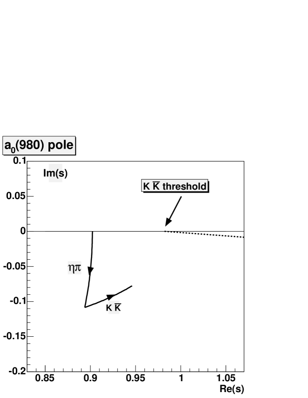
Figure 47: Pole positions of a $T$-matrix describing $\pi\eta$ S–wave interactions as a function of the couplings to $\eta\pi$ and $\rm\bar{K}K$.

Figure 47 shows e.g. the $T$-matrix pole position of a $a_{0}(980)$ resonance coupling to $\eta\pi$ and $\rm\bar{K}K$. When the coupling to the final state is set to zero, the pole position falls onto the real axis, and coincides with the $K$–matrix pole, chosen at $900$ MeV. When the coupling to $\eta\pi$ is turned on, the resonances acquires width and the pole moves into the complex plane $\sqrt{s}$ plane. Then the coupling to $\rm\bar{K}K$ is turned on; the resonance gets narrower and the pole approaches the $\rm\bar{K}K$ threshold.

The mass of the resonance as quoted by experiments is the

Table 16: The K–matrix poles of $\!{}^{{\bf?}}$ show a remarkable agreement with the results of the Bonn model $\!{}^{{\bf?}}$, version B. There is an additional pole at $1400\pm 200$ MeV, far from the real axis (i.e. $\sim 1000$ MeV broad) which is a flavor singlet and could be the glueball.

K-matrix poles			Bonn model, B
	$a_{0}(980\pm 30)$	$f_{0}(680\pm 50)$		$a_{0}(1057)$	$f_{0}(665)$
$\rm K_{0}^{*}(1230\pm 40)$	$a_{0}(1630\pm 40)$	$f_{0}(1260\pm 30)$	$\rm K_{0}^{*}(1187)$	$a_{0}(1665)$	$f_{0}(1262)$
		$f_{0}(1400\pm 200)$
		$f_{0}(1600)$			$f_{0}(1554)$
$\rm K_{0}^{*}(1885^{+50}_{-100})$			$\rm K_{0}^{*}(1788)$
		$f_{0}(1810\pm 50)$			$f_{0}(1870)$

$T$ matrix pole. Quark models usually do not take into account the couplings to the final state. So we might need to compare the $K$–matrix poles with quark model results.

This comparison is made in Table 16. The $K$–matrix poles come from a series of coupled–channel analyses $\!{}^{{\bf?},{\bf?},{\bf?}}$, mean values and errors are estimates provided by one of the authors $\!{}^{{\bf?}}$. The quark model states are from the Bonn model $\!{}^{{\bf?}}$, with the Lorentz structure B of the confinement potential.

There is excellent agreement. The two lowest scalar nonets are identified, and there is one additional state, the $f_{0}(1400\pm 200)$. Its coupling to two pseudoscalar mesons are flavor–blind, it is an isoscalar state. So it can be identified as a scalar glueball. Problematic is the width: it exceeds 2 GeV. In the next section we ask if we can identify a pole of such an enormous width as a resonance. An excellent review of this approach can be found in $\!{}^{{\bf?}}$.

The ‘wide’ glueball scrutinized

Before we continue the discussion we have to introduce a further concept: $s$–channel resonances and $t$–channel exchanges. There are two processes which may contribute to the $\pi\pi$ scattering amplitude: formation of $s$-channel resonances and scattering via $t$-channel exchanges. They are schematically drawn in Figure 48. Scattering processes can be represented by a sum of $s$-channel resonances or by $t$-channel exchanges; in Regge theory this is called duality and is the basis for the Veneziano model. So you may analyze a data set and describe the data by a sum over $s$-channel resonances and get a very good description with a finite number of complex poles in the $\pi\pi$ S-wave scattering amplitude. You could also analyze the data by a summation over $t$-channel exchange amplitudes and also get a good fit. If you add amplitudes for both processes, you run the risk of double counting.

Figure 48: Scattering of two pions (left) via $s$-channel resonances (center) and $t$-channel exchange.

There is a common belief that the interpretation of a pole in the complex scattering energy plane as originating from $s$-, $t$- or $u$-channel phenomenon is a matter of convenience. Indeed, $t$–channel exchanges can lead to resonances; the exchanges represent forces and can lead to binding, can create poles. The $f_{0}(400-1200)$, often called $\sigma(600)$ meson, is certainly present in scattering data with a pole in the complex energy plane. And you may choose to describe this pole as $s$-channel resonance even if its true origin might be $t$-channel exchange. But it is hard to believe that the $\omega$ can be created by $t$–channel forces in the $\rho\pi$ channel. Hence particles may exist which are not created by $t$–channel exchanges. Also the reverse statement is true: not all poles created by exchanges forces need to have particle properties. So, how does one decide if a particular pole in the scattering plane is due to a $s$-channel resonance or to $t$-channel exchanges ?

$s$-channel resonances always have the same ratio of couplings to different final states. The partial widths of the $f_{0}(1500)$ must not depend on the way in which it was produced. This is different for poles generated by $t$-channel exchanges. If properties of a pole depend on the production process, then the pole is not a particle.

Figure 49 shows the $\pi\pi$ scattering amplitude as seen in the GAMS experiment. The modulus of the amplitude shows two dips, at the mass of the $f_{0}(980)$ and $f_{0}(1500)$: intensity is taken from $\pi\pi$ scattering to inelastic channels. The first peak in the scattering amplitude at low energy is the $f_{0}(400-1200)$ and often called $\sigma$-meson; the second bump at 1300 MeV was called $\epsilon(1300)$.

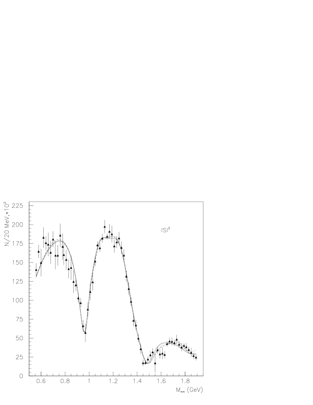
Figure 49: The $\pi\pi$ scattering amplitude measured in the GAMS experiment. From $\!{}^{{\bf?}}$.

The $\pi\pi$ scattering amplitude exhibits a continuously and slowly rising phase and a sudden phase increase at 980 MeV. The rapid phase motion is easily identified with the $f_{0}(980)$, the slowly rising phase can be associated with an $s$-channel resonance which was called $f_{0}(1000)$ by Morgan and Pennington $\!{}^{{\bf?}}$ and the Red Dragon by Minkowski and Ochs $\!{}^{{\bf?}}$. It

extends at least up to 1400 MeV. It has been suggested $\!{}^{{\bf?}}$ that this broad enhancement is the scalar glueball. It seems to agree with the broad glueball discussed in the last section. This broad background amplitude - including the monotonously rising phase - can however well be reproduced by an amplitude for $\rho$ exchange in the $t$-channel. From a fit to the $\pi\pi$ S-wave scattering data even mass and width of the $\rho$ exchanged in the $t$-channel can be determined. So this background amplitude

Figure 50: 4$\pi$ invariant mass spectrum produced by two protons in central collisions. A cut is made on the angle in the transverse direction between the two outgoing protons. Left, 90-135^∘. Right, 135-180^∘. The latter setting corresponds to the so-called glueball filter. The $f_{0}(1500)$ shows up as a dip just like the $f_{0}(980)$ in $\pi\pi$ scattering$\!{}^{{\bf?}}$.

is likely not a $f_{0}(1000)$ $q\bar{q}$ state, nor two mesons, $\sigma(600)$ and $\epsilon(1300)$; it is caused by $\rho$ (and possibly other less important) exchanges in the $t$-channel.

Now, consider figure 50. On the right side, a selection is made for small momentum transfers to the 4$\pi$ system. At small momentum transfer, the $f_{0}(1500)$ is seen as a dip. This resembles very much the data of the GAMS collaboration on $\pi\pi$ scattering (Figure 49). So the question arises if the enhancement seen in the left part of figure 50 is a $q\bar{q}$ resonance. Or can it be traced to $\rho$ and other exchanges in the $t$-channel ? We now argue that the latter is indeed the case.

We now assume that Pomeron-Pomeron scattering can also proceed via $\rho$ exchange in the $t$-channel (figure 51). This $t$-channel amplitude then interferes with the production of the $q\bar{q}$ state $f_{0}(1500)$ producing a dip, very much alike the dip seen at 980 and 1500 MeV in $\pi\pi$ scattering. This conjecture leads to measurable consequences.

Figure 51: Scattering of two Pomerons via $s$-channel resonances and $t$-channel exchange into $\rho\rho$ and into $\sigma\sigma$. Production of $\sigma\sigma$ via $t$–channel exchange seems to be suppressed.

In Pomeron-Pomeron scattering, $\rho$ exchange in the $t$-channel may occur leading to production of two $\rho$ mesons. Isospin conservation does not allow $\sigma\sigma$ production via $\rho$ exchange. Hence we may expect the 4$\pi$ background amplitude not to couple to $\sigma\sigma$.

Figure 52 shows 4$\pi$ invariant mass spectra from the WA102 experiment $\!{}^{{\bf?}}$. A large peak at 1370 MeV is seen followed by a dip in the 1500 MeV region and a further (asymmetric) bump.

Figure 52: 4$\pi$ invariant mass (in GeV) spectra from central production. First row: 2$\pi^{+}$2$\pi^{-}$; second row $\pi^{+}$$\pi^{-}$2$\pi^{0}$; left: $\rho\rho$ S-wave; right: $\sigma\sigma$ S-wave. Third row: $\sigma\sigma$ S-wave in 4$\pi^{0}$ $\!{}^{{\bf?}}$.

The 4$\pi^{0}$ invariant mass spectrum shows the $f_{0}(1500)$ but nearly no background ! The partial wave analysis confirms these findings: it determines contributions from several scalar resonances, the $f_{0}(1370),f_{0}(1500)$ and $f_{0}(1750)$ and a new $f_{0}(1900)$. The partial wave analysis finds $f_{0}(1370)$ decays into $\rho\rho$ but not into $\sigma\sigma$ while the $f_{0}(1500)$ shows both decay modes. In the Crystal Barrel experiment the $f_{0}(1370)$ decays into $\rho\rho$ and into $\sigma\sigma$ with similar strength, see Table 13.

Here we have made an important step. We now understand why the left-hand spectra of figure 52 differ so much from the right-hand spectra. The $\sigma\sigma$ final state can be reached only via $s$-channel resonances and there is only one, the $f_{0}(1500)$. The $\rho$$\rho$ final state is produced by $t$-channel exchanges; they generate the broad enhancement extending over the full accessible mass range. It rises at threshold for 4$\pi$ production and falls off because of the kinematics of central production. High mass systems are suppressed with 1/M².

Notice the similarity of the $f_{0}(1370)$ and the old $\epsilon(1300)$. The relation between these two phenomena is not well understood. The reason that the old $\epsilon(1300)$ was not identified with the $f_{0}(1370)$ lies just here. The $\epsilon(1300)$ was seen in $\pi\pi$ scattering with a small inelasticity, i.e. small coupling to 4$\pi$ while the $f_{0}(1370)$ has small coupling to $\pi\pi$ and a large one to 4$\pi$. This is naturally explained when the 1300 MeV region interacts via $t$-channel exchange. Then $\pi\pi$ goes to $\pi\pi$ , $\rm K\bar{K}$ to $\rm K\bar{K}$, Pomeron-Pomeron to $\pi\pi$ by pion exchange, to $\rho\rho$ via $\rho$ exchange, etc.

Is there no glueball ?

A broad enhancement is observed in the isoscalar S–wave, in $\pi\pi$ and $\rho\rho$ interactions. The enhancement can be interpreted as a scalar glueball $\!{}^{{\bf?}}$. However, at least a large fraction of it must be generated by $t$–channel exchanges, by left–hand cuts. The identification of a glueball component, beneath the intensity generated by $t$–channel exchanges, seems to be hopeless, at least at present. We conclude that there is no ‘narrow’ glueball; a scalar glueball with a width of $\sim 2$ GeV may exist but the experimental methods are not adequate to identify such a broad object as genuine resonance.

Finally, we come back to the question wether the $f_{0}(1370)$ is a genuine resonance. The reaction $\bar{p}p\to\eta 2\pi^{+}2\pi^{-}$ was studied $\!{}^{{\bf?}}$ and it was shown that a large fraction of the final state is reached via the $f_{0}(1370)\eta$ isobar. Due to phase space limitations, no influence by the $f_{0}(980)$ or $f_{0}(1500)$ must be expected. Figure 53 shows amplitude and phase of the $\rho\rho$ system (the $\sigma\sigma$ system shows the same behavior). Amplitude and phase are determined by fitting the data with a $f_{0}(1370)$ of variable width (scanning the mass). For each mass, the fits returns a best complex amplitude. The 4$\pi$ decays give the largest contributions to its width; hence there should be a phase variation by $\pi$. On the contrary, there is not. The $f_{0}(1370)$, the cornerstone of most interpretations of the $f_{0}(1500)$ as scalar glueball, does not behave like a genuine resonance. On the other hand the determination of the phase motion is indirect. The least one can say is that the results in figure 53 do not support the interpretation of the $f_{0}(1370)$ as a normal resonance.

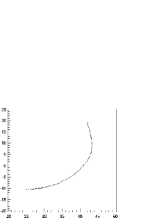
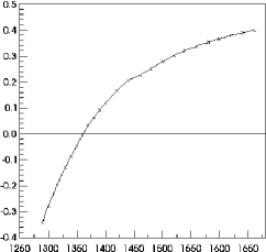
Figure 53: Complex amplitude and phase motion of the $\rho\rho$ scalar isoscalar isobar in $\rm p\bar{p}$ annihilation into $4\pi\eta$. In the mass range from 1300 to 1500 MeV the phase varies by $<0.6$ questioning (but not excluding) the $f_{0}(1370)$ as genuine resonance. The $\sigma\sigma$ (not shown) exhibits the same behavior $\!{}^{{\bf?}}$.

Assuming that the $f_{0}(1370)$ is not a genuine $q\bar{q}$ resonance but generated by $t$–channel exchange, there are left four distinct scalar isoscalar resonances at 980, 1500, 1710 and 2100 MeV. The complicated structure of the resonances with distinct $T$ and $K$-matrix poles may originate from the production and dynamics of hadrons. In “simple” situations like $p\bar{p}$ annihilation in flight into $\pi\eta\eta$ $\!{}^{{\bf?}}$ or radiative J/$\psi$ decays into $4\pi$ $\!{}^{{\bf?}}$ only poles at 1500, 1710, and 2100 MeV show up. These are the “true” quarkonium states. A scalar glueball is not needed to understand the mass spectrum of scalar mesons.

4.6 Hybrids

Hybrids, mesons with an intrinsic gluonic excitation, were first predicted shortly after the development of the bag model  $\!{}^{{\bf?}}$. At that time, hybrids were thought of as $q\bar{q}$ pair in color octet neutralized in color by a constituent gluon $\!{}^{{\bf?},{\bf?}}$. More recent autors expect hybrids as excitations of the gluon fields providing the binding forces between quark and antiquark, as excitations of the color flux tube linking quark and antiquark $\!{}^{{\bf?}}$. The QCD sum rule approach is not as model dependent and finds the lowest $J^{PC}=1^{-+}$ excitation at about 1400 MeV $\!{}^{{\bf?}}$. Due to its inclusive approach, sum rules do not predict if an exotic meson should have a large “$q\bar{q}$ + gluon field” contribution, or if it is dominantly a multiquark state.

The flux tube can have a non–zero orbital–angular–momentum component $\Lambda$ along the $q\bar{q}$ axis, and the following quantum numbers are now possible:

$$S=0\Rightarrow J^{PC}=1^{++},1^{--}$$

$$S=1\Rightarrow J^{PC}=(0,1,2)^{-+},(0,1,2)^{+-}$$

The quantum numbers $J^{PC}=1^{-+},0^{+-},2^{+-},\cdots$ are of particular interest; they are exotic. In the quark model $q\bar{q}$ states cannot be formed with these quantum numbers. Hybrids are expected at masses around 2 GeV and higher $\!{}^{{\bf?}}$ and to decay into two mesons with one of them having one unit of orbital angular momentum $\!{}^{{\bf?}}$.

The $\pi_{1}(1370)$

Indeed an exotic meson has been seen to decay into a $p$-wave $\eta\pi$ system. The quantum numbers in this partial wave are $I^{G}(J^{PC})=1^{-}(1^{-+})$. These are not quantum numbers which are accessible to the $q\bar{q}$ system; they are exotic.

A meson with quantum numbers $I^{G}(J^{PC})=1^{-}(0^{-+})$ is called a $\pi$ and one with $I^{G}(J^{PC})=1^{-}(2^{-+})$ is called $\pi_{2}$. These latter two mesons are well established $q\bar{q}$ mesons. A meson with quantum numbers $I^{G}(J^{PC})=1^{-}(1^{-+})$ is called $\pi_{1}$. Its mass is added to the name in the form $\pi_{1}(1370)$ to identify the meson because there could be (and there are) more than one resonance in this partial wave.

A meson with exotic quantum numbers like the $\pi_{1}(1370)$ cannot be a regular $q\bar{q}$ meson. It must have a more complex structure. It could be a hybrid but it might also be a four-quark ($qq\bar{q}\bar{q}$) resonance. The quantum numbers give no hint which of the two possibilities is realized in nature. Before we discuss arguments in favor of a four-quark assignment let us first have a look at the experimental findings.

At BNL, the reaction

$$\mbox{$\pi^{-}$}\ p\mbox{$\rightarrow$}\ \mbox{$\pi^{-}$}\mbox{$\eta$}\ p$$

was studied at 18 GeV/c $\!{}^{{\bf?},{\bf?}}$. The data shows a large asymmetry in the angular distribution evidencing interference between even and odd angular momentum contributions. Figure 54 shows data and the results of the partial wave analysis. In a scattering process, the $\pi\eta$ system can be produced

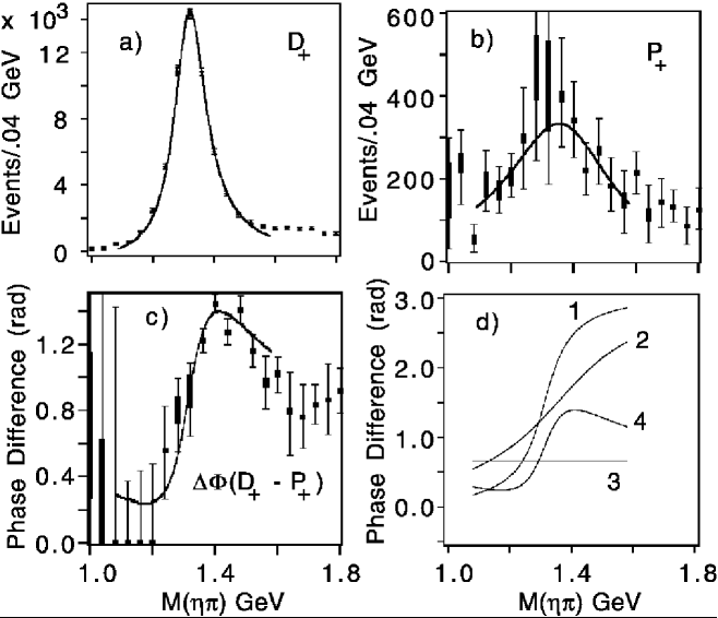
Figure 54: The squared scattering amplitude for the $D^{+}$ (a) and $P^{+}$ (b) waves. The +sign indicates natural parity exchange. The relative phase between the two waves is shown in (c). The lines correspond to the expectation for two Breit-Wigner amplitudes. In (d) the (fitted) phases for the D- (1) and P-wave (2) are shown. The $P$- and $D$-production phases are free parameters in the fits; their difference is plotted as line 3, and - with a different scale - as 4 $\!{}^{{\bf?}}$.

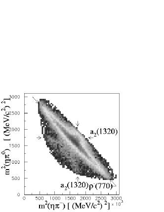
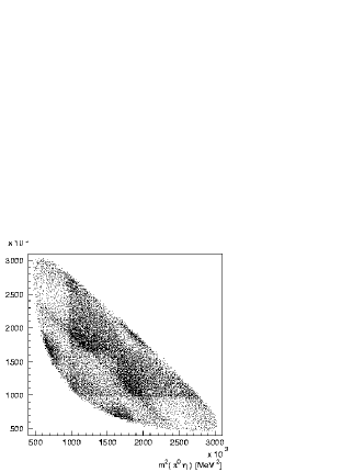
Figure 55: Dalitz plot for the reaction $\bar{p}n\to$ $\pi^{-}$$\pi^{0}$$\eta$ for antiproton annihilation at rest in liquid D₂. Annihilation on quasi-free neutrons is enforced by a cut in the proton momentum ($p_{proton}\leq 100$ MeV/c. The data requires contributions from the $I^{G}(J^{PC})=1^{-}(1^{-+})$ partial wave in the $\eta\pi$ system $\!{}^{{\bf?},{\bf?}}$.

in different partial waves ($S,P,D$ waves). In the $t$-channel quantum numbers are exchanged corresponding to natural ($0^{++},1^{--},2^{++}$) or unnatural ($0^{-+},1^{+-},2^{-+}$) parity. The naturality is a good quantum number for a given partial wave and is added as suffix, + for natural and - for unnatural exchange.

The data is fully compatible with the existence of a resonance in the $I^{G}(J^{PC})=1^{-}(1^{-+})$ partial wave produced via natural parity exchange. Mass and width are fit to values given in Table 17. Since the spin in the final state is one, the exchanged particle cannot have scalar quantum numbers. The resonance is not observed in the charge exchange reaction $\!{}^{{\bf?}}$ (with $\pi^{0}$$\eta$ in the final state), hence the exchanged particle cannot be the $\rho$. The particle exchanged is the $f_{2}(1270)$ (or the tensor part of a Pomeron). The authors of ref. $\!{}^{{\bf?}}$ deduce from the absence of the $\pi_{1}(1370)$ in $\pi^{0}$$\eta$ that the $\pi_{1}(1370)$ might not exist, but what follows is only that it is not produced by $\rho$ exchange. This is further discussed in ref. $\!{}^{{\bf?},{\bf?}}$.

The VES collaboration used $\pi^{-}Be$ interactions at momenta of about 25 GeV/c. They observed a very similar amplitude and phase, in their data from 1993 $\!{}^{{\bf?}}$ and in their more recent data $\!{}^{{\bf?}}$. They cautiously pointed out that background amplitudes can be constructed leading to an acceptable fit to the data in figure 54. Thus they do not see the mandatory need to introduce a new resonance in an exotic partial wave.

The Crystal Barrel Collaboration studied the reaction $\bar{p}n\to\pi^{-}\pi^{0}\eta$ . Figure 55 shows the $\pi^{-}$$\pi^{0}$$\eta$ Dalitz plot. Clearly visible are $\mbox{$\rho$}^{-}\eta$ , $a_{2}(1320)\pi$ with $a_{2}(1320)\to\eta\pi$ (in two charge modes) as intermediate states. A fit with only conventional mesons gives a bad description. The difference between data and predicted Dalitz plot shows a pattern very similar to the contributions expected from the interference of the $\pi_{1}(1370)$ with the amplitudes for production of conventional mesons $\!{}^{{\bf?}}$. Introducing the exotic partial wave, the fit optimizes for values listed in Table 17. Selection rules (and the PWA) attribute the production of the exotic partial wave to the $\bar{p}p$ (${}^{3}S_{1}$) initial atomic state.

A similar analysis on the reaction $\bar{p}p$$\rightarrow$2$\pi^{0}$$\eta$ was carried out. In this case the $\pi_{1}(1370)$ can only be produced from the ${}^{1}S_{0}$ state; its production is considerably reduced in this situation. The small contribution could only be unraveled when data taken by stopping antiprotons in liquid and gaseous H₂ was analyzed. In these two data sets the fraction of annihilation contributions from atomic S and P states is different (their ratio is known from cascade models). Thus S and P wave contributions are constrained. It is only under these conditions that positive evidence for the small contribution from the exotic partial wave could be found $\!{}^{{\bf?}}$, see however ref $\!{}^{{\bf?}}$.

In a partial wave analysis of $\bar{\textrm{p}}\textrm{n}\to\pi^{-}3\pi^{0}$ a $\pi_{1}(1370)$ is seen at slightly higher mass, but with a production characteristic distinctively different from the $\pi_{1}(1370)$ seen in $\pi\eta$ $\!{}^{{\bf?}}$. Hence it is listed as separate exotic meson in Table 17.

Table 17: Evidence for J${}^{\textrm{PC}}$ = $1^{-+}$ exotics. States supposed to be distinct are separated by double–lines. The six entries in the 1600 to 1700 MeV range might be one or two states.

Experiment	mass (MeV/c2)	width (MeV/c2)	decay mode	reaction
BNL $\!{}^{{\bf?}}$	1370 $\pm$ 16 ${}^{+\,\,\,\,\,\,50}_{-\,\,\,\,\,\,30}$	385 $\pm$ 40 ${}^{+\,\,\,65}_{-105}$	$\eta\pi$	$\pi^{-}\textrm{p}\to\eta\pi^{-}\textrm{p}$
BNL $\!{}^{{\bf?}}$	1359 $\,{}^{+\,\,\,\,\,16}_{-\,\,\,\,\,14}$ $\,{}^{+\,\,\,\,\,10}_{-\,\,\,\,\,24}$	314 $\,{}^{+31}_{-29}$ $\,\,\,\,{}^{+\,\,9}_{-66}$	$\eta\pi$	$\pi^{-}\textrm{p}\to\eta\pi^{-}\textrm{p}$
CBar $\!{}^{{\bf?}}$	1400 $\pm$ 20 $\pm$ 20	310 $\pm$ 50 ${}^{+50}_{-30}$	$\eta\pi$	$\bar{\textrm{p}}\textrm{n}\to\pi^{-}\pi^{0}\eta$
CBar $\!{}^{{\bf?}}$	1360 $\pm$ 25	220 $\pm$ 90	$\eta\pi$	$\bar{\textrm{p}}\textrm{p}\to\pi^{0}\pi^{0}\eta$
CBar $\!{}^{{\bf?}}$	$\sim$1440	$\sim$400	$\rho\pi$	$\bar{\textrm{p}}\textrm{n}\to\pi^{-}3\pi^{0}$
BNL $\!{}^{{\bf?}}$	1593 $\pm$ 8 ${}^{+29}_{-47}$	168 $\pm$ 20 ${}^{+150}_{-\,\,\,12}$	$\rho\pi$	$\pi^{-}\textrm{p}\to\pi^{+}\pi^{-}\pi^{-}\textrm{p}$
BNL $\!{}^{{\bf?}}$	1596 $\pm$ 8	387 $\pm$ 23	$\eta^{\prime}\pi$	$\pi^{-}\textrm{p}\to\pi^{-}\eta^{\prime}\textrm{p}$
VES $\!{}^{{\bf?}}$	1610 $\pm$ 20	290 $\pm$ 30	$\rho\pi,\eta^{\prime}\pi$	$\pi^{-}$N$\to\pi^{-}\eta^{\prime}$N
BNL $\!{}^{{\bf?}}$	1709 $\pm$24$\pm$41	403$\pm$80 $\pm$115	$f_{1}(1285)\pi$	$\pi^{-}\textrm{p}\to\eta\pi^{+}\pi^{-}\pi^{-}\textrm{p}$
BNL $\!{}^{{\bf?}}$	1664 $\pm$8$\pm$4	185 $\pm$ 25 $\pm$12	$b_{1}(1235)\pi$	$\pi^{-}\textrm{p}\to\omega\pi^{0}\pi^{-}\textrm{p}$
CBar $\!{}^{{\bf?}}$	1590$\pm$50	280 $\pm$75	$b_{1}(1235)\pi$	$\bar{\textrm{p}}\textrm{p}\to\pi^{+}\pi^{-}\pi^{0}\omega$
BNL $\!{}^{{\bf?}}$	$\sim$2003$\pm$88$\pm$148	306$\pm$132$\pm$121	$f_{1}(1285)\pi$	$\pi^{-}\textrm{p}\to\eta\pi^{+}\pi^{-}\pi^{-}\textrm{p}$
BNL $\!{}^{{\bf?}}$	2000 $\pm$20$\pm$10	230$\pm$32$\pm$15	$\omega\pi^{0}\pi^{-}$	$\pi^{-}\textrm{p}\to\omega\pi^{0}\pi^{-}\textrm{p}$

The $\pi_{1}(1625)$

The $\pi_{1}(1370)$ is not the only resonance observed in this partial wave. At BNL, the $\eta^{\prime}\pi$ is also observed to exhibit a resonant behavior $\!{}^{{\bf?}}$ at about 1600 MeV. A partial wave analysis of the $\rho\pi$ system $\!{}^{{\bf?}}$ reveals an exotic meson with mass and width given in Table 17.

At Protvino, the $\pi\eta^{\prime}$ , $\rho\pi$ and the $b_{1}(1235)\pi$ systems were studied in a 40 GeV/c $\pi^{-}$ beam. In all three systems a resonant contribution in the exotic $I^{G}(J^{PC})=1^{-}(1^{-+})$ partial wave was found. A combined fit found a mass of $\sim$ 1600 MeV and a width of $\sim$ 300 MeV $\!{}^{{\bf?}}$. Possibly these are three different decay modes of one resonance.

The VES collaboration has carried out a partial wave analysis of data on $\omega\pi\pi$ production. The partial waves $\omega\rho$, $b_{1}(1235)\pi$, $\rho_{3}(1690)\pi$, and $\rho_{1}(1450)\pi$ are included in the wave set. The $2^{+}(\omega\rho)$ wave, shown in figure 56a was found to be a dominant wave with a clear $a_{2}(1320)$ peak and a broad bump at 1.7 GeV. A significant $1^{-}(b_{1}\pi)$ wave shown in figure 56b is observed with a broad bump at 1.6 GeV. In figure 56f an $80^{\circ}$ phase rise of the $1^{-}$-wave phase relative to the $2^{+}$-wave phase is observed, which may be attributed to a $1^{-}$ resonance.

A fit describes the interference pattern satisfactorily as seen in figure 56. The data is consistent with the resonant description of the $1^{-}1^{+}S1(b_{1}\pi)$ with the mass 1.6 GeV and width 0.33 GeV. Other hypotheses, including a partially coherent background, did not result in better fits.

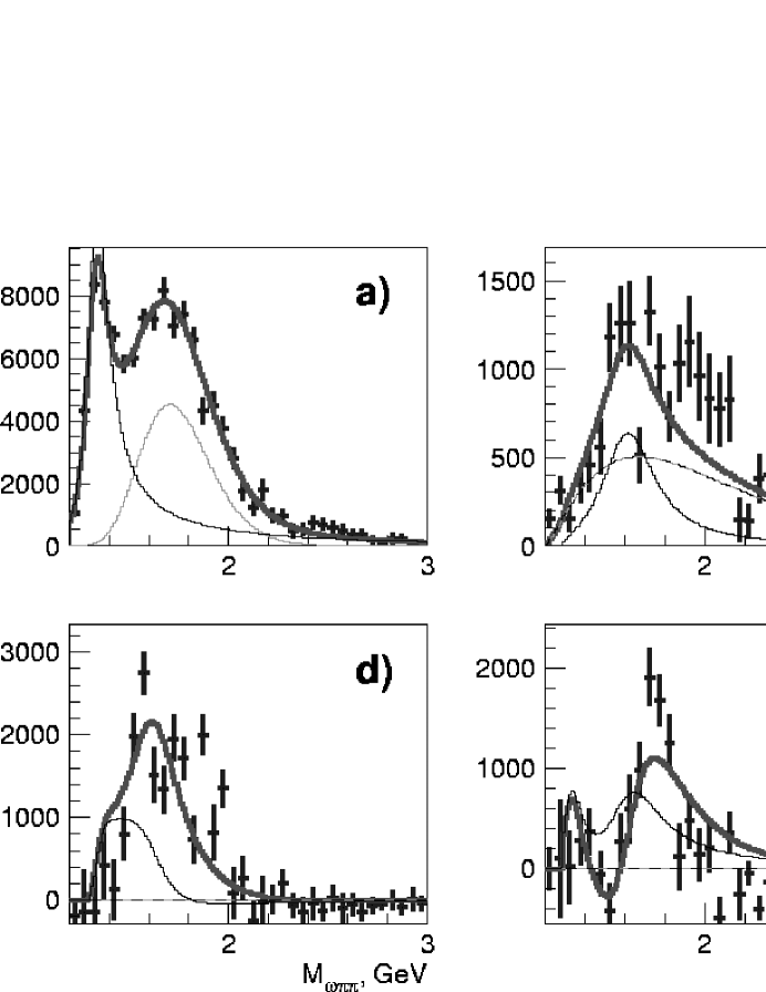
Figure 56:     a) $2^{+}(\omega\rho)$ intensity. b) $1^{-}(b_{1}\pi)$ intensity. c) Coherence parameter. The real d) and imaginary e) parts of their non-diagonal $\rho$-matrix element. f) The $1^{-}$ phase relative to $2^{+}$. The smooth curves are fit results.

Higher-mass exotics

Hybrid mesons are expected to have masses of about 2 GeV and to decay into a P–wave and a S–wave meson. Due to its narrow width, hybrid decays into $\pi^{0}f_{1}(1285)$ are particularly well suited for a search. The two mesons are produced in part with zero orbital angular momentum between them, and this leads to the exotic $I^{G}(J^{PC})=1^{-}(1^{-+})$ partial wave. The amplitude and phase motion in this partial wave (and two other partial waves) are shown in figure 57. A fit with one pole in the $\pi^{0}f_{1}(1285)$ $1^{-+}$ partial wave is obviously not consistent with the data (a fit with no pole is not shown); two poles are required. The results for mass and width are given in Table 17.

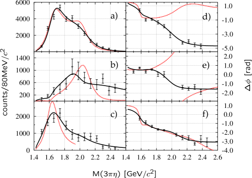
Figure 57: PWA results: $f_{1}(1285)\pi^{-}$ intensity distributions  (a) $1^{++}0^{+}f_{1}\pi^{-}P$, (b) $2^{-+}0^{+}f_{1}\pi^{-}D$, (c) $1^{-+}1^{+}f_{1}\pi^{-}S$ and phase difference distributions (d) $\phi(1^{-+})-\phi(2^{-+})$, (e) $\phi(1^{-+})-\phi(1^{++})$, (f) $\phi(1^{++})-\phi(2^{-+})$. The results from a least squares fit are overlaid as the solid line (two poles in the $1^{-+}f_{1}\pi$ wave) and the dashed line (one pole in the $1^{-+}f_{1}\pi$ wave). From $\!{}^{{\bf?}}$.

The exotic $1^{-+}f_{1}\pi^{-}$ contribution is only observed in positive reflectivity waves, indicating that the process is mediated by exchange of natural parity Reggeons, most likely $\rho(770)$ or $f_{2}(1270)$/Pomeron. An unpublished thesis $\!{}^{{\bf?}}$ reports observation of two $1^{-+}$ exotic mesons decaying into $b_{1}(1235)\pi$. The results are included in Table 17.

Why are so many exotic resonances in this one partial wave ? The number of resonances seems to be three or four: $\pi_{1}(1370)$, $\pi_{1}(1440)$, $\pi_{1}(1625)$, and $\pi_{1}(2000)$. The large number of states in one partial and in such a narrow mass interval is certainly surprising. All have exotic quantum numbers, so they cannot possibly be $q\bar{q}$ states. We now discuss whether they are likely four-quark states or the searched–for hybrid mesons.

The Fock-space expansion

The majority of established mesons can be interpreted as $q\bar{q}$ bound states. This can be an approximation only; the $\rho$-meson e.g. with its large coupling to $\pi\pi$ must have a four-quark component and could as well have contributions from gluonic excitations. The Fock space of the $\rho$ must be more complicated than just $q\bar{q}$. We may write

$$\rho\ =\alpha q\bar{q}+\beta_{1}b\bar{q}q\bar{q}q+...+\gamma_{1}q\bar{q}g+...$$ (27)

where we have used $q\bar{q}g$ as short–hand for a gluonic excitation. The orthogonal states may be shifted into the $\pi\pi$ continuum. Now one might ask, “are the higher-order terms important and what is the relative importance of the $\beta$ and $\gamma$ series ?”

Possibly this question can be answered by truncating the $\alpha$-term. Exotic mesons do not contain a $q\bar{q}$ component and they are rare. Naively we may expect the production of exotics in hadronic reactions to be suppressed by a factor 10 when one of the coefficients, $\alpha_{1}$ or $\beta_{1}$, is of the order 0.3. We thus expect additional states having exotic quantum numbers, quantum numbers which are not accessible to the $q\bar{q}$ system. Their production rate should be suppressed compared to those for regular $q\bar{q}$ mesons. In non-exotic waves the four-quark and hybrid configurations are likely subsumed into the Fock expansion. If we can decide what kind of exotic mesons we observe, four-quarks, hybrids or both, we can say what the most important contributions in (27) are.

SU(3) relations

The $\pi_{1}(1370)$ decays strongly into $\pi\eta$ and the $\pi_{1}(1625)$ into $\pi\eta^{\prime}$; decays of the $\pi_{1}(1370)$ into $\pi\eta^{\prime}$ and of the $\pi_{1}(1625)$ into $\pi\eta$ were not observed or reported. Figure 58 shows the exotic wave for the $\pi\eta$ and $\pi\eta^{\prime}$ systems as a function of their mass; the $\pi\eta$ intensity is concentrated around 1400 MeV, the $\pi\eta^{\prime}$ intensity at 1600 MeV. A resonance decaying into $\pi\eta^{\prime}$ should also decay into $\pi\eta$ , and a $\pi\eta$ resonance should also have a sizable coupling to $\pi\eta^{\prime}$. Why is there such a strange decay pattern ?

Figure 58: The squared scattering amplitude in the $I^{G}(J^{PC})=1^{-}(1^{-+})$ partial wave for the $\pi\eta$ and $\pi\eta^{\prime}$ systems $\!{}^{{\bf?}}$.

We first consider the limit of flavor symmetry. The $\eta$ is supposed to belong to the pseudoscalar octet and the $\eta^{\prime}$ is considered to be a pure singlet SU(3) state. Mixing is neglected. The $\pi_{1}$ states, having isospin one, cannot be isoscalar states. Now I claim that a meson belonging to an octet with exotic quantum numbers $J^{PC}=1^{-+}$ cannot decay into two octet pseudoscalar mesons.

The argument goes as follows: decays of particles belonging to an octet of states into two other octet mesons, decays of the type $8\mbox{$\rightarrow$}8\otimes 8$, may have symmetric or antisymmetric couplings. The two octets can be combined using symmetric structure constants $d_{ijk}$ or antisymmetric structure constants $f_{ijk}$. The decay $\pi_{1}(1370)$ into two pseudoscalar mesons is governed by the symmetric couplings. SU(3) demands the decay amplitude for $\pi_{1}$ decays into two pseudoscalar mesons not to change sign when the two mesons are exchanged. The orbital angular momentum $l=1$ between the two mesons requires the opposite. The two mesons must be in a state $\pi\eta-\eta\pi$. Both requirements cannot be fulfilled at the same time: the decay of a $\pi_{1}$ which belongs to an SU(3) octet into two octet pseudoscalar mesons is forbidden $\!{}^{{\bf?}}$.

There are immediate consequences. Let us begin with the $\pi_{1}(1625)$ and assume that it belongs to an octet of states. Then it must decay into $\pi\eta^{\prime}$ while the decay into $\pi\eta$ is forbidden. This is precisely what we see. But what happens in case of the $\pi_{1}(1370)$ ? It does decay into $\pi\eta$, why ? As we have seen, it cannot belong to an SU(3) octet; it must belong to a SU(3) decuplet $10$ or $\bar{10}$. As member of a decuplet, it cannot decay into $\pi\eta^{\prime}$, into an octet and a singlet meson, and it cannot possibly be a hybrid since gluonic excitations do not contribute to the flavor. Mesonic hybrids can only be SU(3) singlets or octets. The strange phenomenon that the $\pi_{1}(1625)$ does not decay into $\pi\eta$ thus provides the clue for the interpretation of the $\pi_{1}(1370)$ as a four–quark (decuplet) state.

The above arguments hold in the limit of flavor symmetry. Due to $\eta-\eta^{\prime}$ mixing, the exotic $\pi_{1}(1625)$ could decay into $\eta\pi$ via the small singlet component of the $\eta$. A small coupling of the $\pi_{1}(1370)$ to $\eta^{\prime}\pi$ is also possible.

Four-quark states in SU(3)

In the limit of SU(3) symmetry, the $\pi_{1}(1370)$ with its large $\pi\eta$ decay rate must belong to a decuplet and must hence be a four-quark state. The $\pi_{1}(1625)$ must belong to an octet of states and could thus be a hybrid. There is no rigid argument against this conjecture. However, the mass difference between the $\pi_{1}(1370)$ and $\pi_{1}(1625)$ is typical for SU(3) multiplet splitting. It has the same order of magnitude as the octet-decuplet splitting in baryon spectroscopy, only the mass ordering is reversed.

Let us discuss how we can construct a decuplet of states from two quarks and two antiquarks. Two quarks in flavor 3 combine to $3\otimes 3=\bar{3}+6$, two antiquarks to $3+\bar{6}$. Now we construct

$$(\bar{3}+6)\otimes(3+\bar{6})=\bar{3}\otimes 3+\bar{3}\otimes\bar{6}+6\otimes 3+6\otimes\bar{6}$$

$$=1+8+8+10+8+\bar{10}+1+8+27$$

We can construct $10+\bar{10}$ and $10-\bar{10}$ multiplets and four different octets. A large number of different states with the same quantum numbers should be expected from four-quark states.

4.7 Exotic(s) summary

Several exotic mesons are observed, all in one partial wave $I^{G}(J^{PC})=1^{-}(1^{-+})$. The decay pattern of the two resonances at 1400 and 1600 MeV suggests that at least the $\pi_{1}(1370)$ should be a four-quark resonance belonging to a decuplet of states. Then further resonances with quantum numbers $I^{G}(J^{PC})=1^{-}(1^{-+})$ are to be expected and may have been found.

Even though there is no argument against the hypothesis that one of the other observed resonances could be a hybrid, there is at present no experimental support for this hypothesis. Once Pandora’s box of four-quark states has been opened, it is very hard to establish experimentally that mesons with gluonic excitations be found in an experiment.

Finally, do glueballs exist ? This is still an unresolved issue ! We do find natural explanations for the spectrum without request for the presence of a glueball while all interpretations of the spectrum of scalar resonances (which necessitates a scalar glueball) contradict some experimental results, or make questionable assumptions. Of course it is very difficult or even impossible to prove that glueballs and hybrids do not exist. There is, however, no positive evidence that they are needed to understand low–energy hadron physics.

5 Baryon spectroscopy

Baryon resonances have been studied since the early 50’s and a wealth of information is available. Still there are many open questions. The Particle Data Group lists more than 100 baryon resonances; 85 of them have known spin parity but only $\sim 50$ of these are well established, with 3^∗ and 4^∗ ratings. The breakdown of baryon resonances according to their SU(3) classification is given in table 18.

Table 18: Status of baryon resonances according to the The Particle Data Group.

Octet	N		$\Sigma$	$\Lambda$	$\Xi$
Decuplet		$\Delta$	$\Sigma$		$\Xi$	$\Omega$
Singlet				$\Lambda$
****	11	7	6	9	2	1
**	3	3	4	5	4	1
*	6	6	8	1	2	2
	2	6	8	3	3	0
No J	-	-	5	-	8	4
Total	22	22	26	18	11	4

5.1 N^∗ and $\Delta^{*}$ resonances

Spin–orbit forces and the multiplet structure

A severe problem of quark models using one–gluon exchange as residual interaction is posed by the absence of spin–orbit interactions. (The residual interaction was defined by the additional interaction between constituent quarks once confinement is taken into account by a linear potential and chiral symmetry breaking by giving quarks an effective mass.) If the $\Delta$–N mass difference is assigned to the magnetic hyperfine interaction, then large spin–orbit splittings are expected, which is in contrast to experimental findings. The conjecture that the Thomas precession may counterbalance spin–orbit forces is an excuse; model calculations do not support the idea $\!{}^{{\bf?}}$. In this section we show that the systematics of baryon masses suggest that the residual interactions are induced by instantons.

The smallness of spin–orbit forces provides a distinctive benefit when the baryon resonances are to be grouped into supermultiplets. In absence of strong spin–orbit splitting, there are multiplets of approximate equal masses – four resonances with $J=L\pm 3/2,L\pm 1/2$ and two resonances with $J=L\pm 1/2$. Often not all of them are experimentally established, so some interpretation of the data is needed. An assignment of all known N^∗ and $\Delta^{*}$ states is suggested in Table 19.

56	S=1/2;L=0;N=0		N${}_{1/2^{+}}$(939)			939 MeV
	S=3/2;L=0;N=0			$\Delta_{3/2^{+}}$(1232)		1232 MeV
70	S=1/2;L=1;N=0		N${}_{1/2^{-}}(1535)$	N${}_{3/2^{-}}(1520)$		1530 MeV
	S=3/2;L=1;N=0		N${}_{1/2^{-}}$(1650)	N${}_{3/2^{-}}(1700)$	N${}_{5/2^{-}}(1675)$	1631 MeV
	S=1/2;L=1;N=0		$\Delta_{1/2^{-}}(1620)$	$\Delta_{3/2^{-}}(1700)$		1631 MeV
70	S=1/2;L=1;N=2		N${}_{1/2^{-}}(2090)$	N${}_{3/2^{-}}(2080)$		2151 MeV
	S=3/2;L=1;N=2		N${}_{1/2^{-}}$	N${}_{3/2^{-}}$	N${}_{5/2^{-}}$	2223 MeV
	S=1/2;L=1;N=2		$\Delta_{1/2^{-}}(2150)$	$\Delta_{3/2^{-}}$		2223 MeV
56	S=1/2;L=1;N=1		N${}_{1/2^{-}}$	N${}_{3/2^{-}}$		1779 MeV
	S=3/2;L=1;N=1		$\Delta_{1/2^{-}}(1900)$	$\Delta_{3/2^{-}}(1940)$	$\Delta_{5/2^{-}}(1930)$	1950 MeV
56	S=1/2;L=2;N=0		N${}_{3/2^{+}}(1720)$	N${}_{5/2^{+}}(1620)$		1779 MeV
	S=3/2;L=2;N=0	$\Delta_{1/2^{+}}(1910)$	$\Delta_{3/2^{+}}(1920)$	$\Delta_{5/2^{+}}(1905)$	$\Delta_{7/2^{+}}(1950)$	1950 MeV
70	S=1/2;L=2;N=0		N${}_{3/2^{+}}$	N${}_{5/2^{+}}$		1866 MeV
	S=3/2;L=2;N=0	N${}_{1/2^{+}}$	N${}_{3/2^{+}}(1900)$	N${}_{5/2^{+}}(2000)$	N${}_{7/2^{+}}(1990)$	1950 MeV
	S=1/2;L=2;N=0		$\Delta_{3/2^{+}}$	$\Delta_{5/2^{+}}$		1950 MeV
70	S=1/2;L=3;N=0		N${}_{5/2^{-}}$	N${}_{7/2^{-}}$		2151 MeV
	S=3/2;L=3;N=0	N${}_{3/2^{-}}$	N${}_{5/2^{-}}(2200)$	N${}_{7/2^{-}}(2190)$	N${}_{9/2^{-}}(2250)$	2223 MeV
	S=1/2;L=3;N=0		$\Delta_{5/2^{-}}$	$\Delta_{7/2^{-}}(2200)$		2223 MeV
56	S=1/2;L=3;N=1		N${}_{5/2^{-}}$	N${}_{7/2^{-}}$		2334 MeV
	S=3/2;L=3;N=1	$\Delta_{3/2^{-}}$	$\Delta_{5/2^{-}}(2350)$	$\Delta_{7/2^{-}}$	$\Delta_{9/2^{-}}(2400)$	2467 MeV
56	S=1/2;L=4;N=0		N${}_{7/2^{+}}$	N${}_{9/2^{+}}(2220)$		2334 MeV
	S=3/2;L=4;N=0	$\Delta_{5/2^{+}}$	$\Delta_{7/2^{+}}(2390)$	$\Delta_{9/2^{+}}(2300)$	$\Delta_{11/2^{+}}(2420)$	2467 MeV
70	S=1/2;L=5;N=0		N${}_{9/2^{-}}$	N${}_{11/2^{-}}(2600)$		2629 MeV
56	S=3/2;L=5;N=1	$\Delta_{7/2^{-}}$	$\Delta_{9/2^{-}}$	$\Delta_{11/2^{-}}$	$\Delta_{13/2^{-}}(2750)$	2893 MeV
56	S=1/2;L=6;N=0		N${}_{11/2^{+}}$	N${}_{13/2^{+}}(2700)$		2781 MeV
	S=3/2;L=6;N=0	$\Delta_{9/2^{+}}$	$\Delta_{11/2^{+}}$	$\Delta_{13/2^{+}}$	$\Delta_{15/2^{+}}(2950)$	2893 MeV
70	S=1/2;L=7;N=0		N${}_{13/2^{-}}$	N${}_{15/2^{-}}$		3033 MeV
56	S=3/2;L=7;N=1	$\Delta_{11/2^{-}}$	$\Delta_{13/2^{-}}$	$\Delta_{15/2^{-}}$	$\Delta_{17/2^{-}}$	3264 MeV
56	S=1/2;L=8;N=0		N${}_{15/2^{+}}$	N${}_{17/2^{+}}$		3165 MeV
	S=3/2;L=8;N=0	$\Delta_{13/2^{+}}$	$\Delta_{15/2^{+}}$	$\Delta_{17/2^{+}}$	$\Delta_{19/2^{+}}$	3264 MeV

Table 19: Multiplet structure of nucleon and $\Delta$ resonances. The table contains all known resonances except radial excitations of the N${}_{1/2^{+}}$(939) and $\Delta_{3/2^{+}}$(1232).

Regge trajectories

The masses of meson- and $\Delta^{*}$ resonances for which all intrinsic angular momenta are aligned ($J=L+1$ and $J=L+3/2$, respectively) fall onto Regge trajectories as we had seen in figure 21. Figure 59 differs from the standard Regge trajectory by plotting the mass square against the orbital angular momentum L instead of J. Since spin-orbit forces are small, the orbital angular momentum is well defined. We choose L to be one variable because this allows us to combine baryons of positive and negative parity. The figure includes $\Delta^{*}$ resonances with intrinsic spin 3/2 and 1/2 (the latter ones must have negative parity !), and N^∗ intrinsic quark spin 3/2.

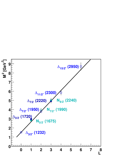
Figure 59: Regge trajectory for $\Delta^{*}$ resonances with with intrinsic spin $S=1/2$ and $3/2$, and for N^∗’s with spin $S=3/2$. They all fall onto the same trajectory.

Not included in figure 59 are the nucleon and nucleon resonances with spin 1/2. In figure 60 we compare the squared masses of positive- and negative-parity baryon resonances having intrinsic spin $S=1/2$ to the standard Regge trajectory of figure 59. All resonances are lower in mass compared to the trajectory, except the $\Delta^{*}$ states. The mass shifts are discrete. The shift (in mass square) for negative–parity singlet states is 0.99. For positive–parity octet states it equals 0.66, and for negative–parity octet states 0.33. For negative–parity decuplet states the shift is 0. The $\Delta$–nucleon mass shift is e.g. given by

$$\rm s_{i}=M^{2}_{\Delta(1232)}-M^{2}_{nucleon}=0.64.$$ (28)

We note that nucleons with S=1/2 are shifted in mass and nucleons with spin 3/2 are not. $\Delta$ excitations do not have this spin-dependent mass shift. The mass shift occurs only for baryons having wave-functions antisymmetric w.r.t. the exchange of two quarks in both, in spin and in flavor (not only in their spin–flavor wave function). As we have seen in section 3, this is the selection rule for instanton–induced interactions acting only between pairs of quarks antisymmetric w.r.t. their exchange in spin and flavor $\!{}^{{\bf?}}$. We consider the even-odd staggering of figure 60 as the most striking evidence for the role of instanton–induced interactions in low-energy strong interactions (or of other field configurations with a non–vanishing winding number).

Radial excitations

Some partial waves show a second resonance at a higher mass. The best known example is the Roper resonance, the N${}_{1/2^{+}}$(1440). Its mass is rather low compared to most calculations because in the harmonic oscillator description of baryon resonances it is found in the second excitation band ($N=2$). Table 20 lists consecutive states and their mass–square splitting, all compatible with the N–Roper mass difference.

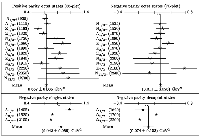
Figure 60: Mass square shift (in GeV²) of spin-1/2 baryons w.r.t. the Regge trajectory $\rm M^{2}=M_{\Delta}^{2}+{n_{s}}/3\cdot M_{s}^{2}+a\,(L+N)$ defined by baryons with S=3/2 (hyperfine splitting). The mass shifts scale as 1 : 1/2 : 3/2 : 0 times $\rm M_{\Delta}^{2}-M_{\rm N}^{2}$ as we proposed in mass formula (29) $\!{}^{{\bf?}}$.

Table 20: Radial excitations of baryon resonances

Baryon	$\delta\rm M^{2}\ (GeV^{2})$		Baryon	$\delta\rm M^{2}\ (GeV^{2})$
N${}_{1/2^{+}}(939)$			$\Delta_{3/2^{+}}(1232)$
N${}_{1/2^{+}}(1440)$	$1\cdot 1.18$		$\Delta_{3/2^{+}}(1600)$	$1\cdot 1.04$
N${}_{1/2^{+}}(1710)$	$2\cdot 1.02$		$\Delta_{3/2^{+}}(1920)$	$2\cdot 1.08$
N${}_{1/2^{+}}(2100)$	$3\cdot 1.18$
$\Delta_{1/2^{-}}(1620)$			$\Delta_{3/2^{-}}(1700)$
$\Delta_{1/2^{-}}(1900)$	$1\cdot 0.99$		$\Delta_{3/2^{-}}(1940)$	$1\cdot 0.87$
$\Delta_{1/2^{-}}(2150)$	$2\cdot 1.00$
N${}_{1/2^{-}}(1530)$			N${}_{3/2^{-}}(1520)$
N${}_{1/2^{-}}$(1530)			N${}_{3/2^{-}}$(1530)
N${}_{1/2^{-}}(2090)$	$2\cdot 1.01$		N${}_{3/2^{-}}(2080)$	$2\cdot 1.01$
$\Lambda_{1/2^{+}}(1115)$			$\Sigma_{1/2^{+}}(1193)$
$\Lambda_{1/2^{+}}(1600)$	$1\cdot 1.24$		$\Sigma_{1/2^{+}}(1560)$	$1\cdot 1.04$
$\Lambda_{1/2^{+}}(1810)$	$2\cdot 0.98$		$\Sigma_{1/2^{+}}(1880)$	$1\cdot 1.06$

Resonances with strangeness

The mass of a baryon increases with its strangeness content. The dependence is usually assumed to be linear. Here the squared baryon masses are given as linear functions of the strangeness. There are small deviations from the interpolation between the $\Omega$ and the $\Delta$ when using squared masses. A linear mass interpolation does not yield a better agreement.

5.2 Observations and conclusions

We now recall the basic experimental observations and draw obvious conclusions from these facts.

1. The slope of the Regge trajectory for meson- and $\Delta$-excitations is identical. Baryon resonances are quark-diquark excitations.

2. $\ \Delta^{*}$ resonances with S=1/2 and S=3/2 fall onto the same Regge trajectory. There is no significant spin-spin splitting due to color-magnetic interactions. Gluon exchange, often assumed to be responsible for the N-$\Delta$ splitting, should also lead to a mass shift of the $\Delta_{1/2^{-}}$(1620) and $\Delta_{3/2^{-}}$(1700) relative to the leading Regge trajectory, in the same order of magnitude as in the case of the N-$\Delta$ splitting. This is not the case. Gluon exchange is not responsible for the N-$\Delta$ splitting.

3. N and $\Delta$ resonances with spin S=3/2 lie on a common Regge trajectory. There is no genuine octet-decuplet splitting. For spin-3/2 resonances, there is no interaction associated with the SU(6) multiplet structure.

4. N^∗s and $\Delta^{*}$s can be grouped into super-multiplets with defined orbital angular momenta L and intrinsic spin S, but different total angular momentum J. There is no significant spin-orbit ($\vec{\rm L}\cdot\vec{\rm S}$) interaction. This is again an argument against a large role of gluon exchange forces (even though the spin-orbit splitting due to one-gluon exchange could be compensated by the Thomas precession in the confinement potential).

5. Octet baryons with intrinsic spin 1/2 have a shift in the squared mass. The shift is larger (by a factor 2) for even orbital angular momenta than for odd angular momenta. Wave functions of octet baryons with spin 1/2 contain a component $\rm\left(q_{1}q_{2}-q_{2}q_{1}\right)\left(\uparrow\downarrow\ -\downarrow\uparrow\right)$. The mass shift is proportional to this component. Instanton interactions act on quark pairs antisymmetric in their spin and their flavor wave function with respect to their exchange. The mass shifts shown in figure 59 manifest the importance of instanton–induced interactions in the baryon spectrum.

6. Daughter trajectories have the same slope as the main trajectory and an intercept higher by $a=1.142$ GeV² per $\ n$, both for mesons and baryons. The similarity of the spacings between radial excitations of mesons and baryons supports the interpretation of baryon resonances as quark-diquark excitations.

These observations allow us to write down a simple formula $\!{}^{{\bf?}}$ reproducing all 100 (but four) masses of baryon resonances observed so far.

$$\rm M^{2}=M_{\Delta}^{2}+\frac{n_{s}}{3}\cdot M_{s}^{2}+a\cdot(L+N)-s_{i}\cdot I_{sym},$$ (29)

where

$$\rm M_{s}^{2}=\left(M_{\Omega}^{2}-M_{\Delta}^{2}\right),\qquad\ \rm s_{i}=\left(M_{\Delta}^{2}-M_{\rm N}^{2}\right),$$

$n_{s}$ is the number of strange quarks in a baryon, and L is the intrinsic orbital angular momentum. N is the principal quantum number (we start with N=0 for the ground state); L+2N gives the harmonic-oscillator band N. $\rm I_{sym}$ is the fraction of the wave function (normalized to the nucleon wave function) antisymmetric in spin and flavor. It is given by

$\rm I_{sym}=$	1.0	for S=1/2 and	octet in 56-plet;
$\rm I_{sym}=$	0.5	for S=1/2 and	octet in 70-plet;
$\rm I_{sym}=$	1.5	for S=1/2 and	singlet;
$\rm I_{sym}=$	0	otherwise.

$\rm M_{N},M_{\Delta},M_{\Omega}$ are input parameters taken from PDG; $a=1.142$/GeV² is the Regge slope as determined from the meson spectrum.

Data and the mass formula (29) are compared in Tables 21 to 24. To estimate if the agreement is good, we need errors. In the Particle Data Listings these are only given for well known baryons. We could relate the errors to the widths, but the widths are also known only with large uncertainties. We estimate the widths of a baryon according to

$$\Gamma_{\rm B}=\frac{1}{4}Q$$ (30)

were $Q$ is the largest decay momentum (into N$\pi$ for N^∗ and $\Delta^{*}$) of a resonance. The calculated widths are also given in Tables 21 to 24. One quarter of the width is assumed to be the error in mass. A resonance may decay and rescatter into the resonance again in the form of loop diagrams. Such virtual decays lead to hadronic shifts. We estimate that these could be on the order of 1/4 of the line width. With this definition the ground state masses have no error and some errors become very small. Hence we adopt a model error of 30 MeV which is added quadratically to the error due to hadronic shifts.

Table 21: Mass spectrum of N resonances. See caption of Table (22).

Baryon	Status	$\rm D_{L}$	N	Mass	(29)	$\Gamma$	(30)	$\sigma$	$\chi^{2}$
N${}_{1/2^{+}}(939)$	****	$(56,^{2}8)_{0}$	0	939	-	-	-	-	-
N${}_{1/2^{+}}(1440)$	****	$(56,^{2}8)_{0}$	1	1450	1423	250-450	87	37	0.53
N${}_{1/2^{+}}(1710)$	***	$(56,^{2}8)_{0}$	2	1710	1779	50-250	176	53	1.69
1N${}_{1/2^{+}}(2100)$	*	$(56,^{2}8)_{0}$	2	2100	2076	-	251	70	0.12
N${}_{1/2^{-}}(1535)$	****	$(70,^{2}8)_{1}$	0	1538	1530	100-250	114	41	0.04
N${}_{3/2^{-}}(1520)$	****	$(70,^{2}8)_{1}$	0	1523	1530	110-135	114	41	0.03
N${}_{1/2^{-}}(1650)$	****	$(70,^{4}8)_{1}$	0	1660	1631	145-190	139	46	0.4
N${}_{3/2^{-}}(1700)$	***	$(70,^{4}8)_{1}$	0	1700	1631	50-150	139	46	2.25
N${}_{5/2^{-}}(1675)$	****	$(70,^{4}8)_{1}$	0	1678	1631	140-180	139	46	1.04
N${}_{3/2^{+}}(1720)$	****	$(56,^{2}8)_{2}$	0	1700	1779	100-200	176	53	2.22
N${}_{5/2^{+}}(1680)$	****	$(56,^{2}8)_{2}$	0	1683	1779	120-140	176	53	3.28
N${}_{3/2^{+}}(1900)$	**	$(70,^{4}8)_{2}$	0	1900	1950	-	219	62	0.65
N${}_{5/2^{+}}(2000)$	**	$(70,^{4}8)_{2}$	0	2000	1950	-	219	62	0.65
N${}_{7/2^{+}}(1990)$	**	$(70,^{4}8)_{2}$	0	1990	1950	-	219	62	0.42
N${}_{1/2^{-}}(2090)$	*	$(70,^{2}8)_{1}$	2	2090	2151	-	269	74	0.68
N${}_{3/2^{-}}(2080)$	**	$(70,^{2}8)_{1}$	2	2080	2151	-	269	74	0.92
N${}_{5/2^{-}}(2200)$	**	$(70,^{2}8)_{3}$	0	2220	2151	-	269	74	0.87
N${}_{7/2^{-}}(2190)$	****	$(70,^{2}8)_{3}$	0	2150	2151	350-550	269	74	0
N${}_{9/2^{-}}(2250)$	****	$(70,^{4}8)_{3}$	0	2240	2223	290-470	287	78	0.05
N${}_{9/2^{+}}(2220)$	****	$(56,^{2}8)_{4}$	0	2245	2334	320-550	315	84	1.12
N${}_{11/2^{-}}(2600)$	***	$(70,^{2}8)_{5}$	0	2650	2629	500-800	389	102	0.04
N${}_{13/2^{+}}(2700)$	**	$(56,^{2}8)_{6}$	0	2700	2781	-	427	111	0.53
						dof:	21	$\sum\chi^{2}$:	17.53

¹ Based on its mass, the N${}_{1/2^{+}}(2100)$ is likely a radial excitation. It could also be the $(70,^{4}8)_{2}$ N${}_{1/2^{+}}$ state expected at 1950 MeV. The SAPHIR collaboration suggested a N${}_{1/2^{+}}$ at 1986 MeV $\!{}^{{\bf?}}$ which would, if confirmed, be a natural partner to complete the quartet of L=2, S=3/2 nucleon resonances.

The mass formula reproduces not only the masses of N^∗, $\Delta^{*}$’s, $\Sigma^{*}$’s and $\Lambda^{*}$’s which are reproduced in tables here, it is also compatible with the few entries for $\Xi^{*}$’s $\Omega^{*}$’s.

Table 22: Mass spectrum of $\Delta$ resonances. A baryon resonance is characterized by its $\rm J^{P}$ as subscript and its nominal mass (in parenthesis). The PDG rating is given by the number of *’s. Its classification into multiplets is discussed in section (6). The PDG lists a range of acceptable values, we give the central mass (in MeV), compared to the predicted mass from eq. (29). We list the PDG range of acceptable widths $\Gamma$ and compare them to eq. (30). The width parameterization is only used to estimate errors. The mass errors $\sigma$ are given by $\sigma^{2}=\frac{\Gamma^{2}}{16}+30^{2}$ where the first error allows for hadronic mass shifts on the order of 1/4 of the line width, the second one for uncertainties in the mass formula. The last column gives the $\chi^{2}$ contribution from the mass comparison. The $\chi^{2}$s are summed up and compared to the degrees of freedom in the last column.

Baryon	Status	$\rm D_{L}$	N	Mass	(29)	$\Gamma$	(30)	$\sigma$	$\chi^{2}$
$\Delta_{3/2^{+}}(1232)$	****	$(56,^{4}10)_{0}$	0	1232	1232	-	-	-	-
$\Delta_{3/2^{+}}(1600)$	***	$(56,^{4}10)_{0}$	1	1625	1631	250-450	139	46	0.02
$\Delta_{1/2^{+}}(1750)$	*	$(70,^{2}10)_{0}$	1	1750	1631	-	139	46	6.69
$\Delta_{1/2^{-}}(1620)$	****	$(70,^{2}10)_{1}$	0	1645	1631	120-180	139	46	0.09
$\Delta_{3/2^{-}}(1700)$	****	$(70,^{2}10)_{1}$	0	1720	1631	200-400	139	46	3.74
$\Delta_{1/2^{-}}(1900)$	**	$(56,^{4}10)_{1}$	1	1900	1950	140-240	219	62	0.65
$\Delta_{3/2^{-}}(1940)$	*	$(56,^{4}10)_{1}$	1	1940	1950	-	219	62	0.03
$\Delta_{5/2^{-}}(1930)$	***	$(56,^{4}10)_{1}$	1	1945	1950	250-450	219	62	0.01
$\Delta_{1/2^{+}}(1910)$	****	$(56,^{4}10)_{2}$	0	1895	1950	190-270	219	62	0.79
$\Delta_{3/2^{+}}(1920)$	***	$(56,^{4}10)_{2}$	0	1935	1950	150-300	219	62	0.06
$\Delta_{5/2^{+}}(1905)$	****	$(56,^{4}10)_{2}$	0	1895	1950	280-440	219	62	0.79
$\Delta_{7/2^{+}}(1950)$	****	$(56,^{4}10)_{2}$	0	1950	1950	290-350	219	62	0
$\Delta_{1/2^{-}}(2150)$	*	$(70,^{2}10)_{1}$	2	2150	2223	-	287	78	0.88
$\Delta_{7/2^{-}}(2200)$	*	$(70,^{2}10)_{3}$	0	2200	2223	-	287	78	0.09
${}^{1}\Delta_{5/2^{+}}(2000)$	**	$(70,^{2}10)_{2}$	1	2200	2223	-	287	78	0.09
$\Delta_{5/2^{-}}(2350)$	*	$(56,^{4}10)_{3}$	1	2350	2467	-	348	92	1.62
$\Delta_{9/2^{-}}(2400)$	**	$(56,^{4}10)_{3}$	1	2400	2467	-	348	92	0.53
$\Delta_{7/2^{+}}(2390)$	*	$(56,^{4}10)_{4}$	0	2390	2467	-	348	92	0.7
$\Delta_{9/2^{+}}(2300)$	**	$(56,^{4}10)_{4}$	0	2300	2467	-	348	92	3.3
$\Delta_{11/2^{+}}(2420)$	****	$(56,^{4}10)_{4}$	0	2400	2467	300-500	348	92	0.53
$\Delta_{13/2^{-}}(2750)$	**	$(56,^{4}10)_{5}$	1	2750	2893	-	455	118	1.47
$\Delta_{15/2^{+}}(2950)$	**	$(56,^{4}10)_{6}$	0	2950	2893	-	455	118	0.23
						dof:	21	$\sum\chi^{2}$:	22.31

¹The PDG quotes two entries, at 1752 and 2200 MeV, respectively, and gives 2000 as ”our estimate”. We use the higher mass value for our comparison.

Table 23: Mass spectrum of $\Sigma$ resonances. See caption of Table (21).

Baryon	Status	$\rm D_{L}$	N	Mass	(29)	$\Gamma$	(30)	$\sigma$	$\chi^{2}$
$\Sigma_{1/2^{+}}(1193)$	****	$(56,^{2}8)_{0}$	0	1193	1144	-	-	30	2.67
$\Sigma_{3/2^{+}}(1385)$	****	$(56,^{4}10)_{0}$	0	1384	1394	-	-	30	0.11
$\Sigma(1480)$	*
$\Sigma(1560)$	**	$(56,^{2}8)_{0}$	1	1560	1565	-	32	31	0.03
$\Sigma_{1/2^{+}}(1660)$	***	$(70,^{2}8)_{0}$	1	1660	1664	40-200	57	33	0.01
$\Sigma_{1/2^{+}}(1770)$	*	$(70,^{2}10)_{0}$	1	1770	1757	-	80	36	0.13
$\Sigma_{1/2^{+}}(1880)$	**	$(56,^{2}8)_{0}$	2	1880	1895	-	115	42	0.13
$\Sigma_{1/2^{-}}(1620)$	**	$(70,^{2}8)_{1}$	0	1620	1664	-	57	33	1.78
$\Sigma_{3/2^{-}}(1580)$	**	$(70,^{2}8)_{1}$	0	1580	1664	-	57	33	6.48
$\Sigma(1690)$	**	$(70,^{2}10)_{1}$	0	1690	1757	-	80	36	3.46
$\Sigma_{1/2^{-}}(1750)$	***	$(70,^{4}8)_{1}$	0	1765	1757	60-160	80	36	0.05
$\Sigma_{3/2^{-}}(1670)$	****	$(70,^{4}8)_{1}$	0	1675	1757	40-80	80	36	5.19
$\Sigma_{5/2^{-}}(1775)$	****	$(70,^{4}8)_{1}$	0	1775	1757	105-135	80	36	0.25
$\Sigma_{1/2^{-}}(2000)$	*	$(70,^{2}8)_{1}$	1	2000	1977	-	135	45	0.26
$\Sigma_{3/2^{-}}(1940)$	***	$(70,^{2}8)_{1}$	1	1925	1977	150-300	135	45	1.34
$\Sigma_{3/2^{+}}(1840)$	*	$(56,^{2}8)_{2}$	0	1840	1895	-	115	42	1.71
$\Sigma_{5/2^{+}}(1915)$	****	$(56,^{2}8)_{2}$	0	1918	1895	80-160	115	42	0.3
${}^{1}\Sigma_{3/2^{+}}(2080)$	**	$(56,^{4}10)_{2}$	0	2080	2056	-	155	49	0.24
${}^{1}\Sigma_{5/2^{+}}(2070)$	*	$(56,^{4}10)_{2}$	0	2070	2056	-	155	49	0.06
${}^{1}\Sigma_{7/2^{+}}(2030)$	****	$(56,^{4}10)_{2}$	0	2033	2056	150-200	155	49	0.22
$\Sigma(2250)$	***	$(70,^{2}8)_{3}$	0	2245	2248	60-150	203	59	0
$\Sigma_{7/2^{-}}(2100)$	*	$(70,^{2}8)_{3}$	0	2100	2248	-	203	59	6.29
$\Sigma(2455)$	**	$(56,^{2}8)_{4}$	0	2455	2424	-	247	69	0.2
$\Sigma(2620)$	**	$(70,^{2}8)_{5}$	0	2620	2708	-	318	85	1.07
$\Sigma(3000)$	*	$(56,^{2}8)_{6}$	0	3000	2857	-	355	94	2.31
$\Sigma(3170)$	*	$(70,^{2}8)_{7}$	0	3170	3102	-	416	108	0.4
						dof:	25	$\sum\chi^{2}$:	34.69

¹ These three resonances, and the missing $\Sigma_{1/2^{+}}$, can belong to the octet or to the decuplet; the mass formula (29) predicts identical masses.

Table 24: Mass spectrum of $\Lambda$ resonances. See caption of Table (22).

Baryon	Status	$\rm D_{L}$	N	Mass	(29)	$\Gamma$	(30)	$\sigma$	$\chi^{2}$
$\Lambda_{1/2^{+}}(1115)$	****	$(56,^{2}8)_{0}$	0	1116	1144	-	-	30	0.87
$\Lambda_{1/2^{+}}(1600)$	***	$(56,^{2}8)_{0}$	1	1630	1565	50-250	32	31	4.4
$\Lambda_{1/2^{+}}(1810)$	***	$(56,^{2}8)_{0}$	2	1800	1895	50-250	115	42	5.12
$\Lambda_{1/2^{-}}(1405)$	****	$(70,^{2}1)_{1}$	0	1407	1460	50	6	30	3.12
$\Lambda_{3/2^{-}}(1520)$	****	$(70,^{2}1)_{1}$	0	1520	1460	16	6	30	4
$\Lambda_{1/2^{-}}(1670)$	****	$(70,^{2}8)_{1}$	0	1670	1664	25-50	57	33	0.03
$\Lambda_{3/2^{-}}(1690)$	****	$(70,^{2}8)_{1}$	0	1690	1664	50-70	57	33	0.62
$\Lambda_{1/2^{-}}(1800)$	***	$(70,^{4}8)_{1}$	0	1785	1757	200-400	80	36	0.6
$\Lambda_{5/2^{-}}(1830)$	****	$(70,^{4}8)_{1}$	0	1820	1757	60-110	80	36	3.06
$\Lambda_{3/2^{+}}(1890)$	****	$(56,^{2}8)_{2}$	0	1880	1895	60-200	115	42	0.13
$\Lambda_{5/2^{+}}(1820)$	****	$(56,^{2}8)_{2}$	0	1820	1895	70-90	115	42	3.19
$\Lambda(2000)$	*	$(70,^{4}8)_{2}$	0	2000	2056	-	155	49	1.31
$\Lambda_{5/2^{+}}(2110)$	***	$(70,^{4}8)_{2}$	0	2115	2056	150-250	155	49	1.45
$\Lambda_{7/2^{+}}(2020)$	*	$(70,^{4}8)_{2}$	0	2020	2056	-	155	49	0.54
$\Lambda_{7/2^{-}}(2100)$	****	$(70,^{2}1)_{3}$	0	2100	2101	100-250	166	51	0
$\Lambda_{3/2^{-}}(2325)$	*	$(70,^{2}8)_{1}$	2	2325	2248	-	203	59	1.7
$\Lambda_{9/2^{+}}(2350)$	***	$(56,^{2}8)_{4}$	0	2355	2424	100-250	247	69	1
$\Lambda(2585)$	**	$(70,^{4}8)_{2}$	0	2585	2551	-	279	76	0.2
						dof:	18	$\sum\chi^{2}$:	31.34

It is remarkable that all observed resonances are well reproduced by the mass formula. If we assume that the mass formula calculates $(qqq)$–baryon masses, there is no hot candidate left for other forms of baryons which are predicted by models: hybrid baryons or pentaquarks. These will be the topic of sections 5.5.

5.3 The ’missing resonances’

A three–body system supports a rich dynamical spectrum. This can be seen when looking at Table 25 which lists the wave functions in the harmonic oscillator basis. For each of these realizations there is the full decomposition in SU(6). Hence a multitude of baryon resonances is expected. The number of known resonances is much smaller: this is the problem of the so–called ’missing resonances’. Many more resonances are expected to exist than observed experimentally. This is not a problem of an incomplete stamp collection. A large number of resonances are missing and we do not know the guiding principle which leads to the observation of some resonances and the non–observation of others.

There are two possible solutions. One is that the resonances have not been discovered so far. In particular one can argue that some of the resonances may have a weak coupling only to the N$\pi$ channel. Since nearly all N^∗ and $\Delta^{*}$ resonances were discovered in $\pi$N scattering, they may have escaped discovery. These resonances are however predicted to have normal coupling to $\gamma$N. Photo–production of baryon resonances and detection of multibody final states should therefore reveal if these states exist or not.

Table 25: Harmonic oscillator wave functions as excitations in the $\lambda$ and $\rho$ oscillator basis. Baryons can be excited orbitally ($l_{i}$) and radially ($n_{i}$). Radial excitations carry two $\hbar\omega$, the excitation to the Roper with $n_{1}=1$ is therefore in the 2^nd band ($N=2$). The two orbital angular momenta $l_{i}$ couple to the total angular momentum $L$. The shell quantum number $N$ is hence $N=l_{1}+l_{2}+2n_{1}+2n_{2}$. The multiplicity is given by ${\rm n}=2L+1$. The $\sum\rm n$ gives the total number of realizations in a shell. A smaller number of wave functions can be realized if it is required that only one of the two oscillators is excited.

$N$	n	$l_{1}$	$l_{2}$	$n_{1}$	$n_{2}$	$L$	$\sum\rm n$	$N$	n	$l_{1}$	$l_{2}$	$n_{1}$	$n_{2}$	$L$	$\sum\rm n$
0	1	0	0	0	0	0	1 / 1	4	9	4	0	0	0	4
1	3	1	0	0	0	1		4	9	0	4	0	0	4
1	3	0	1	0	0	1	6 / 6	4	21	3	1	0	0	2,3,4
2	5	2	0	0	0	2		4	21	1	3	0	0	2,3,4
2	5	0	2	0	0	2		4	25	2	2	0	0	1,2-4
2	5	1	1	0	0	2		4	5	2	0	1	0	2
2	3	1	1	0	0	1		4	5	0	2	1	0	2
2	1	1	1	0	0	0		4	9	1	1	1	0	0,1,2
2	1	0	0	1	0	0		4	5	2	0	0	1	2
2	1	0	0	0	1	0	21 / 12	4	5	0	2	0	1	2
3	7	3	0	0	0	3		4	9	1	1	0	1	0,1,2
3	7	0	3	0	0	3		4	1	0	0	2	0	0
3	15	2	1	0	0	1,2,3		4	1	0	0	0	2	0
3	15	1	2	0	0	1,2,3		4	1	0	0	1	1	0	126 / 30
3	3	1	0	1	0	1
3	3	0	1	1	0	1
3	3	1	0	0	1	1
3	3	0	1	0	1	1	56 / 20

Could it be that these resonances do not exist at all ? One often discussed solution of the ’missing resonances’ problem is the possibility that two quarks in a baryon form a quasi–stable diquark $\!{}^{{\bf?}}$. Such scenarios are back in the center of the scientific discussion since Lipkin and Karliner $\!{}^{{\bf?},{\bf?},{\bf?}}$ Jaffe and Wilzcek $\!{}^{{\bf?}}$ proposed a diquark model to explain the exotic properties of the $\Theta^{+}(1540)$.

The single-quark excitation hypothesis

Below, a possibility is sketched how the large number of expected states might be reduced without using ’exotic’ assumptions. It is a sketch only which will require systematic study and application to all partial waves. Likely, the reduction of states will not be sufficient in all partial waves, so it is a first step only. Consider $\rm L=2$, $\rm N=1$ as example. Both oscillators can be excited to have quantum numbers $l_{\rho},l_{\lambda},n_{\rho},n_{\lambda}$. L$=2$, N$=1$ belong to the 4^th excitation band. The configurations which can contribute are listed below:

$${(l_{\rho},n_{\rho},l_{\lambda},n_{\lambda})=(2,1,0,0)=|0>} \qquad;\qquad {(0,0,2,1)=|8>}$$

$${(l_{\rho},n_{\rho},l_{\lambda},n_{\lambda})=(2,0,0,1)=|2>} \qquad;\qquad {(0,1,2,0)=|6>}$$

$${(l_{\rho},n_{\rho},l_{\lambda},n_{\lambda})=(2,0,2,0)=|4>} \qquad;\qquad$$

$${(l_{\rho},n_{\rho},l_{\lambda},n_{\lambda})=(3,0,1,0)=|1>} \qquad;\qquad {(1,0,3,0)=|7>}$$

$${(l_{\rho},n_{\rho},l_{\lambda},n_{\lambda})=(1,1,1,0)=|3>} \qquad;\qquad {(1,0,1,1)=|5>}$$

Note that only the wave functions $|0>$ and $|8>$ contain single–quark excitations, in the other 7 functions, both oscillators are excited. These wave functions do not yet obey the Pauli principle. New wave functions need to be constructed having defined symmetry under exchange of two quarks. These are given by:

$$\ |\ S0> = \ +\ \sqrt{\ \frac{1}{6}}\cdot{\frac{1}{\sqrt{2}}(\ |\ 0>+\ \ |\ 8>)}\ +\ \sqrt{\frac{7}{18}}\cdot\frac{1}{\sqrt{2}}(\ |\ 2>+\ \ |\ 6>)\ -\ \sqrt{\ \frac{4}{9}}\ |\ 4>$$

$$\ |\ S1> = \ +\ \sqrt{\frac{7}{12}}\cdot{\frac{1}{\sqrt{2}}(\ |\ 0>+\ \ |\ 8>)}\ +\ \sqrt{\frac{1}{36}}\cdot\frac{1}{\sqrt{2}}(\ |\ 2>+\ \ |\ 6>)\ +\ \sqrt{\frac{7}{18}}\ |\ 4>$$

$$\ |\ MS0> = \ +\ \sqrt{\ \frac{1}{4}}\cdot\,{\frac{1}{\sqrt{2}}(\ |\ 0>+\ \ |\ 8>)}\,\ -\ \sqrt{\frac{7}{12}}\cdot\frac{1}{\sqrt{2}}(\ |\ 2>+\ \ |\ 6>)\ -\ \sqrt{\ \frac{1}{6}}\ |\ 4>$$

$$\ |\ MS1> = \ +\ \sqrt{\frac{3}{10}}\cdot{\frac{1}{\sqrt{2}}(\ |\ 0>-\ \ |\ 8>)}\ -\ \sqrt{\frac{7}{10}}\cdot\frac{1}{\sqrt{2}}(\ |\ 2>-\ \ |\ 6>)$$

$$\ |\ MS2> = \ +\ \sqrt{\frac{7}{10}}\cdot{\frac{1}{\sqrt{2}}(\ |\ 0>-\ \ |\ 8>)}\ +\ \sqrt{\frac{3}{10}}\cdot\frac{1}{\sqrt{2}}(\ |\ 2>-\ \ |\ 6>)$$

$$\ |\ MA0> = \ +\ \sqrt{\frac{4}{25}}\cdot\frac{1}{\sqrt{2}}(\ |\ 1>+\ \ |\ 7>)\ -\ \sqrt{\frac{21}{25}}\cdot\frac{1}{\sqrt{2}}(\ |\ 3>+\ \ |\ 5>)$$

$$\ |\ MA1> = \ -\ \sqrt{\frac{21}{25}}\cdot\frac{1}{\sqrt{2}}(\ |\ 1>+\ \ |\ 7>)\ -\ \sqrt{\frac{4}{25}}\cdot\frac{1}{\sqrt{2}}(\ |\ 3>+\ \ |\ 5>)$$

$$\ |\ MA2> = \ +\ \sqrt{\frac{3}{10}}\cdot\frac{1}{\sqrt{2}}(\ |\ 1>-\ \ |\ 7>)\ +\ \sqrt{\frac{7}{10}}\cdot\frac{1}{\sqrt{2}}(\ |\ 3>-\ \ |\ 5>)$$

$$\ |\ A0> = \ -\ \sqrt{\frac{7}{10}}\cdot\frac{1}{\sqrt{2}}(\ |\ 1>-\ \ |\ 7>)\ +\ \sqrt{\frac{3}{10}}\cdot\frac{1}{\sqrt{2}}(\ |\ 3>-\ \ |\ 5>)$$

None of these wave functions contains single–quark excitations only. But we can now assume that in the process of baryon production the initial state after excitation of a baryon is given by $\frac{1}{\sqrt{2}}{\ |\ 0>}\pm\frac{1}{\sqrt{2}}{\ |\ 8>}$. This is not an energy eigenstate. But in case that the masses of states $|0>$, $|4>$, $|6>$ and $|8>$ are not too different, a coherent superposition will be formed, with a mean energy and there are only two baryons instead of 9. Those states composed of $|1>$, $|2>$, $|5>$ and $|7>$ cannot be reached when the single-quark excitation hypothesis holds true. The conjecture has the following consequences:

1. Resonances with symmetric wave functions ($S0$, $S1$ and $MS0$) and with mixed symmetric wave functions ($MS1$ and $MS2$) are coherently excited

   $${\frac{1}{\sqrt{2}}(|0>\ +\ |8>)} = \sqrt{\frac{1}{6}}|S0>\ +\ \sqrt{\frac{7}{12}}|S1>\ +\ \frac{1}{2}|MS0>,$$

   $${\frac{1}{\sqrt{2}}(|0>\ -\ |8>)} = \sqrt{\frac{3}{10}}|MS1>\ +\ \sqrt{\frac{7}{10}}|MS2>.$$

2. Baryon resonances are wave packets with defined phase but uncertain in quantum number ($\delta\phi\cdot\delta n\sim\hbar$).

3. We expect a large reduction in the number of states.

4. Resonances with antisymmetric and mixed antisymmetric wave functions are not excited.

5. Only relevant quantum numbers are $L=l_{\rho}+l_{\lambda}$ and $N=n_{\rho}+n_{\lambda}$.

6. These are used in the baryon mass formula.

Hybrid baryons

In the same way as the gluon flux tube in a meson can possibly be excited (leading to hybrid mesons), also hybrid baryon states can be constructed where the flux tubes are connecting the quarks are excited. The color flux meets in a junction (in a Mercedes star configuration) which plays, for every quark, the role of the antiquark. A model calculation $\!{}^{{\bf?}}$ gave a rich spectrum; certainly the problem of ’missing resonances’ is aggravated. Capstick and Page used an adiabatic approximation for the quark motion, quarks were confined by a linear potential; flux tubes and junction were modeled by attracting beads vibrating in various string modes. The Coulomb potential from one-gluon exchange was assumed the same in conventional and hybrid baryons, and spin-dependent terms were neglected. Before splitting due to one–gluon exchange interactions, hybrids with quark orbital angular momenta $L_{q}=0,1,2$ have masses 1980, 2340 and 2620 MeV respectively. Hyperfine (contact plus tensor) interactions split the $N$ hybrids down and the $\Delta$ hybrids up, so that the lowest N hybrid mass becomes 1870 MeV. The model error on this mass was estimated to be less than $\pm 100$ MeV.

5.4 New directions

The overwhelming majority of data on baryon resonances, their masses, widths, and partial decay widths comes from pion elastic scattering off nucleons. This experimental technique demonstrated to be very powerful but, it is restricted to baryon resonances with sufficiently large coupling to the N$\pi$ system. For high baryon masses, the N$\pi$ couplings become small, and other experimental techniques are mandatory. Photo–production of high–mass states is predicted to be less suppressed than formation via pion–proton scattering.

Baryon resonances with high mass can be expected to decay via cascades. The resonance $\rm N(2220)H_{19}$ can decay, with a probability of 10-20%, via pion emission into N$\pi$. The N$\pi$ system then has an orbital angular momentum $\ell=6$. In the decay sequence $\rm N(2220)H_{19}\to N(1675)D_{15}\pi$, and $\rm N(1675)D_{15}\to N\pi$ the angular momenta are $\ell_{1}=4$ and $\ell_{2}=1$. Hence the angular momentum barrier for these decays is smaller. For a study of such sequential decays there are two requirements. First, instrumentations are needed which detect multiparticle final states. Second, one needs to be sure that photo–production can identify resonances also when pion scattering data are scarce.

At the Bonn electron accelerator ELSA, data on photoproduction of $\pi^{0}$ and $\eta$ mesons were taken with the Crystal Barrel detector (used before at LEAR). Figure 61 shows those for $\eta$ production $\!{}^{{\bf?}}$. These data, plus GRAAL data on the beam asymmetry of photoproduction of $\pi^{0}$ and $\eta$ mesons, were fitted with an isobar model. The results of the fits which are still preliminary, are collected in table 26.

Table 26: Masses and widths of N^∗ and $\Delta^{*}$ resonances as determined from data on photoproduction of $\pi^{0}$ and $\eta$ mesons, and comparison with PDG values $\!{}^{{\bf?}}$.

P r e l i m i n a r y

N∗	M (MeV)	$\Gamma$ (MeV)	PDG mass	PDG width
${\rm N(1520)D_{13}}$	$\sim 1530$	$\sim 110$	$1520$	$120^{+15}_{-10}$
${\rm N(1535)S_{11}}$	$\sim 1511$	$\sim 170$	$1505\pm 10$	$170\pm 80$
${\rm N(1650)S_{11}}$	$\sim 1636$	$\sim 180$	$1660\pm 20$	$160\pm 10$
${\rm N(1675)D_{15}}$	$\sim 1650$	$\sim 140$	$1670-1685$	$140-180$
${\rm N(1680)F_{15}}$	$\sim 1670$	$\sim 100$	$1680^{+10}_{-5}$	$130\pm 10$
${\rm N(1700)D_{13}}$	$\sim 1695$	$\sim 220$	$1650-1750$	$50-150$
${\rm N(1720)P_{13}}$	$\sim 1735$	$\sim 250$	$1720^{+30}_{-70}$	$250\pm 50$
${\rm N(1900)P_{13}}$	$\sim 1920$	$\sim 230$	$\sim 1900$	$\sim 500$
${\rm N(2070)D_{15}}$	$\sim 2070$	$\sim 335$	-	-
${\rm\Delta(1232)P_{33}}$	$\sim 1234$	$\sim 120$	$1232\pm 2$	$120\pm 5$
${\rm\Delta(1600)P_{33}}$	$\sim 1585$	$\sim 120$	$1232\pm 2$	$120\pm 5$
${\rm\Delta(1700)D_{33}}$	$\sim 1700$	$\sim 210$	$1670-1770$	$200-400$
${\rm\Delta(1750)P_{31}}$	$\sim 1710$	$\sim 250$	$\sim 1750$	$\sim 300$
${\rm\Delta(1905)F_{35}}$	$\sim 1870$	$\sim 280$	$1870-1920$	$280-440$
${\rm\Delta(1920)P_{33}}$	$\sim 1960$	$\sim 230$	$1900-1970$	$150-300$
${\rm\Delta(1950)F_{37}}$	$\sim 1940$	$\sim 260$	$1940-1960$	$290-350$
${\rm\Delta(2260)P_{33}}$	$\sim 2260$	$\sim 400$	-	-

The agreement between the results from photoproduction with those of the PDG, mostly $\pi$N elastic scattering, is remarkable. Two new resonances are suggested.

One of the new resonances is the $\rm N(2070)D_{15}$. Surprisingly, the evidence for this resonance comes from the $\eta$ data of figure 61. Other resonances which are seen to contribute strongly to figure 61 are the $\rm N(1535)S_{11}$ and the $\rm N(1730)P_{13}$. These three resonances decay into N$\eta$ with orbital angular momenta $L=0,1,2$. Their possible spectroscopic assignments are depicted in figure 62.

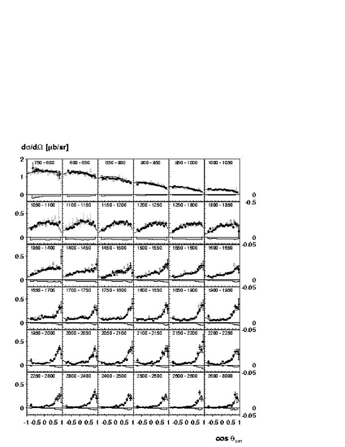
Figure 61: Differential cross sections for the reaction $\gamma p\to p\eta$ at CB-ELSA $\!{}^{{\bf?}}$.

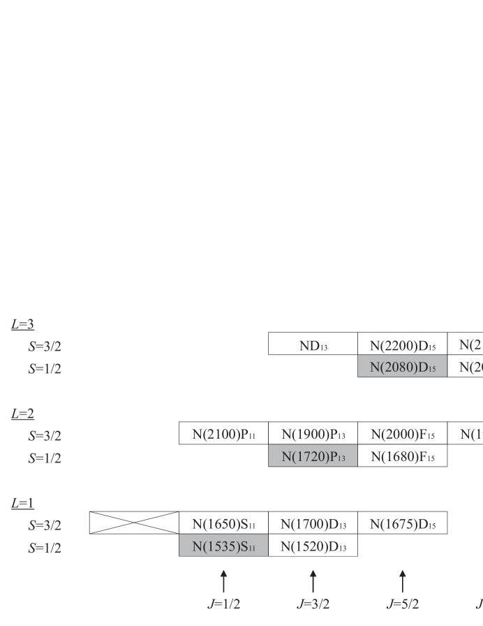
Figure 62: Low–lying baryon multiplets. The dominant contributions are orbital angular momentum excitations $\ell=1,2,3$ where the intrinsic(quark) orbital angular momentum $\vec{\ell}$ couples to the total quark spin, $s=1/2$ or $s=3/2$, to a doublet or quartet of states. The states with $J=\ell-s,s=1/2$ couple strongly to N$\eta$. There is no explanation so far for this regularity.

Cascades of baryon resonances can already been seen in data on $\gamma p\to p2\pi^{0}$. Figure 63 shows the $p\pi^{0}$ invariant mass distribution for events in which the total mass falls into the 2000–2200 MeV mass range.

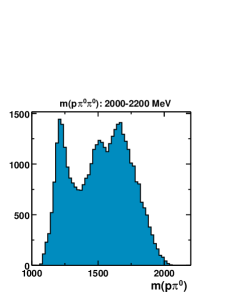
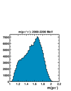
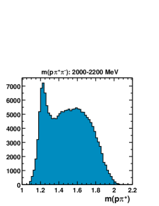
Figure 63: The $p\pi$ invariant mass distributions for the reaction $\gamma p\to p2\pi$. Left: CB-ELSA data on $\gamma p\to p2\pi^{0}$. Plotted is the $p\pi^{0}$ invariant mass. Then CLAS data on $\gamma p\to p\pi^{+}\pi^{-}$. Shown are the $p\pi^{-}$ invariant (center) and $p\pi^{+}$ (right) invariant mass. The total mass ( or $\sqrt{s}$) was restricted to 2000–2200 MeV.

Clearly, high mass baryon resonance cascade down via intermediate resonances. Often to the $\Delta(1232)$, see figure 63, left and right panels, but also via the $\rm N(1520)D_{13}$. This cascade can be seen in the left panel of figure 63. Thus cascade processes open a new chance to investigate the spectrum of baryon resonances.

5.5 Pentaquarks

An exotic baryon with positive strangeness $S=+1$ was found by Nakano and collaborators at LEPS in Japan $\!{}^{{\bf?}}$, and has since then been confirmed by several other experiments. As resonance with positive strangeness it must contain an $\bar{s}$ quark; to maintain a baryon number one, the minimum quark model configuration of the $\Theta^{+}(1540)$ requires five quarks, it is called pentaquark. The resonance was found to have a mass of $\sim 1540$ MeV and a narrow width $\leq 10$ MeV. The name $\Theta^{+}(1540)$ was adopted.

LEPS experiment

Nakano et al. $\!{}^{{\bf?}}$ observed the $\Theta^{+}(1540)$ in a study of photo-production off neutrons in the reaction

$$\rm\gamma n\to K^{+}K^{-}n$$ (31)

using neutrons in carbon nuclei of a plastic scintillator. The primary aim of the experiment was the study of $\Phi$ photo–production of protons using a liquid H₂ target.

The experiment was performed at the Laser Electron Photon facility at SPring8 (LEPS) in Japan. This apparatus produces high-energy photons by Compton back-scattering of laser photons off a 8 GeV electron beam in the SPring-8 storage ring. Using a 351 nm Ar laser, photons with a maximum energy of 2.4 GeV were produced. The scattered electrons were momentum- analyzed by a bending magnet and detected by a tagging counter inside the ring; this allowed the photon energy to be determined with a resolution of 15 MeV. The flux of tagged photons in the energy range from 1.5 to 2.4 GeV was $10^{6}$/s. Charged particles were tracked through a magnetic field, electrons and positrons were vetoed by an aerogel Cerenkov counter, Kaons were identified in a time–of–flight system.

Figure 64: The LEPS experiment: a, the vertex distribution and cuts to select events produced in the scintillator and in H₂. b, the $\rm K^{+}K^{-}$ invariant mass distribution for events in H₂ (dashed line) and in the scintillator (solid line) $\!{}^{{\bf?}}$.

Figure 65: The LEPS experiment: a, the scatter–plot $MM_{\rm\gamma K^{+}}$ versus $MM_{\rm\gamma K^{+}\pi^{-}}$ shows the effect of the Fermi motion. b, the corrected missing mass distribution $MM^{c}_{\rm\gamma K^{\pm}}$ (solid line) shows a clear $\Sigma^{-}$ hardly seen in the uncorrected spectrum (dashed line). The dotted line shows Monte Carlo simulations of the $\Sigma^{-}$ $\!{}^{{\bf?}}$.

Figure 66: The LEPS experiment, corrected missing mass distributions for $\rm K^{+}K^{-}$ production. a, $MM^{c}_{\rm\gamma K^{+}}$ for data on H₂ (dashed) showing the $\Lambda(1520)$ and on Carbon with a detected proton (solid). b, $MM^{c}_{\rm\gamma K^{-}}$ from H₂ (dashed) and on Carbon (solid). The latter peak is assigned to reaction $\gamma n\to\Theta^{+}\rm K^{-};\Theta^{+}\to nK^{+}$ $\!{}^{{\bf?}}$.

The photon energy was known from the tagging and the target nucleon was assumed to be at rest with the mean nucleon rest mass; hence from the momentum of the kaon pair, the momentum and direction of the final state nucleon could be calculated. The silicon-strip detector (SSD) was able to detect protons, but is blind to neutrons. Figure 66 shows the vertex distribution and the $\rm K^{+}K^{-}$ invariant mass distribution for events where a proton was identified.

In a next step, only those events were retained where the calculated nucleon momentum and direction would lead to a hit in SSD but where no matching proton was found. From this sample, the reactions $\rm\gamma n\to nK^{+}\pi^{-}$ and $\rm\gamma n\to nK^{+}K^{-}$ were identified. The former reaction proceeds via the intermediate state $\rm K^{+}\Sigma^{-}$. Both, the $\Sigma^{-}$ and n mass can be determined from the missing masses recoiling against the $\rm\gamma K^{+}$ or $\rm\gamma K^{+}\pi^{-}$, respectively. The two masses are both smeared out by the Fermi motion, the missing mass corrected for the Fermi motion is calculated as

$$MM^{c}_{\rm\gamma K^{\pm}}=MM_{\rm\gamma K^{\pm}}-MM^{c}_{\rm\gamma K^{+}K^{-}}+M_{N}.$$ (32)

Nakano et al. looked for the $\Theta^{+}$ in the $\rm K^{-}$ missing mass distribution again corrected for the neutron Fermi momentum (see figure 66b). A peak was seen at 1540 MeV. The statistical significance of this peak over the background was determined to 4.6$\sigma$. The peak width of 25 MeV was consistent with the experimental resolution, and is only an upper boundary on the true decay width of the state. There is no peak in the corresponding data from the H₂ target.

The SAPHIR experiment

The $\Theta^{+}$ has also been observed in photo–production from protons at the Bonn ELectron Stretcher Accelerator (ELSA) $\!{}^{{\bf?}}$. The reaction:

$$\rm\gamma p\to nK^{+}K^{0}_{s}$$ (33)

was studied with the SAPHIR detector, a large acceptance magnetic spectrometer. The detector has full coverage in the forward direction; thus particles can be detected (and their momentum be measured) even under zero degrees, however, the photon flux is limited to $\sim 10^{6}\gamma$/s. Photons were produced via bremsstrahlung of the

Figure 67: Top: the $n\rm K^{+}$ and $n\rm K^{0}_{s}$ invariant mass distributions. Bottom: The $\pi^{+}\pi^{-}$ and $n\rm K^{+}$ invariant mass distributions after side–bin subtraction of the background under the $\rm K^{0}_{s}$ or $\Theta^{+}(1540)$, respectively. From $\!{}^{{\bf?}}$.

ELSA electron beam in a copper foil radiator and were tagged with energies from 31% to 94% of the incident electron energy, which was 2.8 GeV for the data shown. Liquid hydrogen was used as the target. $\rm K^{0}_{s}$ were reconstructed from their $\pi^{+}\pi^{-}$ decay, and the neutron momentum was obtained from energy and momentum conservation.

A series of kinematical fits was applied to suppress background from competing reactions. Figure 67 shows the resulting $n\rm K^{+}$ and $n\rm K^{0}_{s}$ invariant mass distributions with clear peaks at 1542 MeV and at the $\Lambda(1520)$ invariant mass. The $n\rm K^{+}$ mass spectrum was obtained after a cut in the $\rm K^{0}_{s}$ production angle $cos\theta_{\rm K^{0}_{s}}>0.5$ which reduces the background by a factor four and the signal by about a factor two.

The $\Theta^{+}$ was seen as a peak in the $\rm nK^{+}$ invariant mass distribution, with a statistical significance of 4.8$\sigma$. The mass was measured as $1540\pm 4\pm 2$  MeV, and the width determined to be $\leq$25,MeV, at a 90% confidence level.

The correlation between $\rm K^{0}_{s}$ and the peak in the $n\rm K^{+}$ invariant mass distribution can be seen when the background under the $\rm K^{0}_{s}$ and the $\Theta^{+}$, estimated from side bins, is subtracted (figure 67). The $\Theta^{+}$ is now seen above very few events, probably due to $\Lambda(1520)\rm K^{+}$ production.

The SAPHIR collaboration also searched for an isospin-partner of the $\Theta^{+}$, the doubly-charged $\Theta^{++}$, via the reaction chain:

$$\rm\gamma p\to\Theta^{++}K^{-}\to pK^{+}K^{-}$$ (34)

If the $\Theta^{+}$ would have isospin 1 or 2, we should expect a peak in figure 69 with several 1000 entries. From the absence of such a strong signal in the $\rm pK^{+}$ invariant mass distribution, they concluded that the $\Theta^{+}$ is an isoscalar.

Figure 68: The $p\rm K^{+}$ invariant mass distribution from reaction (34) measured at SAPHIR $\!{}^{{\bf?}}$.

Figure 69: Diagrams which could contribute to $\Theta^{+}(1540)$ production. In the upper diagram, K⁰ exchange requires SU(3) symmetry breaking, K^∗ exchange could be allowed but is suppressed due to its higher mass. A isotensor resonance $\Theta^{+}(1540)$ is only produced via contact interactions.

Diagrams which could contribute to $\Theta^{+}$ production are shown in figure 69. A isotensor resonance is more difficult to produce: the vector component of the photon plus the proton has to combine in a four–point vertex into an isotensor plus isodoublet.

The DIANA experiment

The DIANA collaboration found evidence for the $\Theta^{+}$ resonance from low-energy interactions of $\rm K^{+}$ with nuclei $\!{}^{{\bf?}}$. The data had been collected in 1986 and were re-analyzed recently. A kaon beam of 850 MeV was generated at the ITEP proton synchrotron. The experiment consisted of a 70x70x140 cm bubble chamber filled with liquid Xenon. Beam momentum and target size were chosen to stop the Kaon beam at the end of their range. Figure 70 shows the position along the target where the $\rm K^{+}$ interacted or decayed.

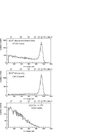
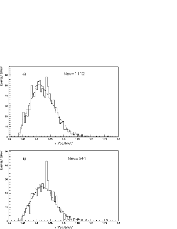
Figure 70: DIANA, left: 850 MeV $\rm K^{+}$ entered a Xe bubble chamber. They may decay in flight, interact with Xe nuclei, or stop at the end of their range. Right: $\rm pK^{0}_{s}$ invariant mass distribution for all events and for those in which proton and $\rm K^{0}_{s}$ were produced with an angle $\theta<100^{\circ}$ w.r.t. the beam direction and back-to-back in the transverse plane $\!{}^{{\bf?}}$.

There was no magnetic field. Charged particles were identified by their ionization tracks and momentum-analyzed by their range in Xenon. DIANA studied the $\rm\Theta^{+}\to pK^{0}_{s}$ decay of the $\Theta^{+}$ by inspecting the $\rm pK^{0}_{s}$ invariant mass distribution in the charge exchange reaction

$$\rm K^{+}Xe\to Xe^{\prime}pK^{0}_{s}.$$ (35)

The distribution is shown in Figure 70. An enhancement is seen at a mass $M=1539\pm 2$ MeV and with a width of $\Gamma<9$ MeV. The statistical significance was 4.4$\sigma$.

Cahn and Trilling $\!{}^{{\bf?}}$ related the number of interacting Kaons to the $\rm K^{+}n$ cross section. Since the integrated cross section (or total number of $\Theta^{+}$) is proportional to the width, they estimated the $\Theta^{+}$ width to 1 MeV.

The CLAS experiment

The CLAS (CEBAF Large Acceptance Spectrometer) collaboration at Jefferson Lab studied photo-production of the $\Theta^{+}$ using a H₂ and D₂ target. In a first experiment liquid deuterium was used. The photons were produced by an electron beam incident on a bremsstrahlung radiator and their energies were determined from a measurement of the energy of the corresponding electrons. Charged-particle tracking was performed in large acceptance drift chambers, and particle identification used a Time-of-Flight detector. The CLAS collaboration studied the reaction $\!{}^{{\bf?}}$:

$$\rm\gamma d\to pnK^{+}K^{-}$$ (36)

using a D₂ target and reaction $\!{}^{{\bf?}}$

$$\rm\gamma p\to nK^{+}K^{-}\pi^{+}.$$ (37)

with a H₂ target. In both cases, the neutron was reconstructed from the kinematics; hence, the momenta of all participating particles are known. Figs. 71 and 72 show diagrams which may contribute to $\Theta^{+}$ production in reaction (36) and (37), respectively.

Figure 71: Two rescattering diagrams that could contribute to $\Theta^{+}$ production in D₂ through final state interactions $\!{}^{{\bf?}}$. The $\Theta^{+}$ is produced independently of the secondary scattering.

Figure 72: $\Theta^{+}$ production in H₂ via K exchange, with and without production of K^∗’s. $Z^{+}$ is an older name of the $\Theta^{+}$ $\!{}^{{\bf?}}$.

Neutrons in the final state were reconstructed from the missing momentum and energy. Events were selected which contained an identified proton, a $\rm K^{+}$ and $\rm K^{-}$ pair, and no other particles. The missing mass spectrum for the selected events showed a clear peak at the neutron mass, with resolution of 9 MeV (see figure 75). The $\rm nK^{+}$ invariant mass distribution (figure 75) exhibits a peak structure which is identified as $\Theta^{+}(1540)$. Known reactions which also produce $\rm K^{+}K^{-}$ pairs, such as $\Phi$–decay, were removed by cuts on the invariant mass of the kaon pair. In general, this is an unnecessary precaution which just reduces the number of events. A sharp peak at 1542 MeV in the $\rm nK^{+}$ invariant mass distribution was seen, with a statistical significance of 5.8$\sigma$. The width was measured to be less than 21 MeV.

Spectator protons do not escape the target, but the detection of the proton was essential to reconstruct the neutron from kinematics. Since they looked for the $\Theta^{+}$ in the $\rm nK^{+}$ invariant mass spectrum, also the neutron participated in the reaction. Hence there was no spectator particle.

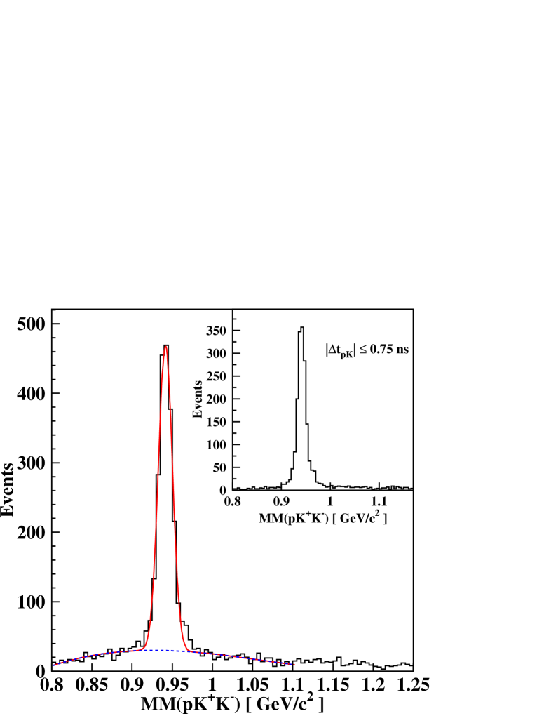
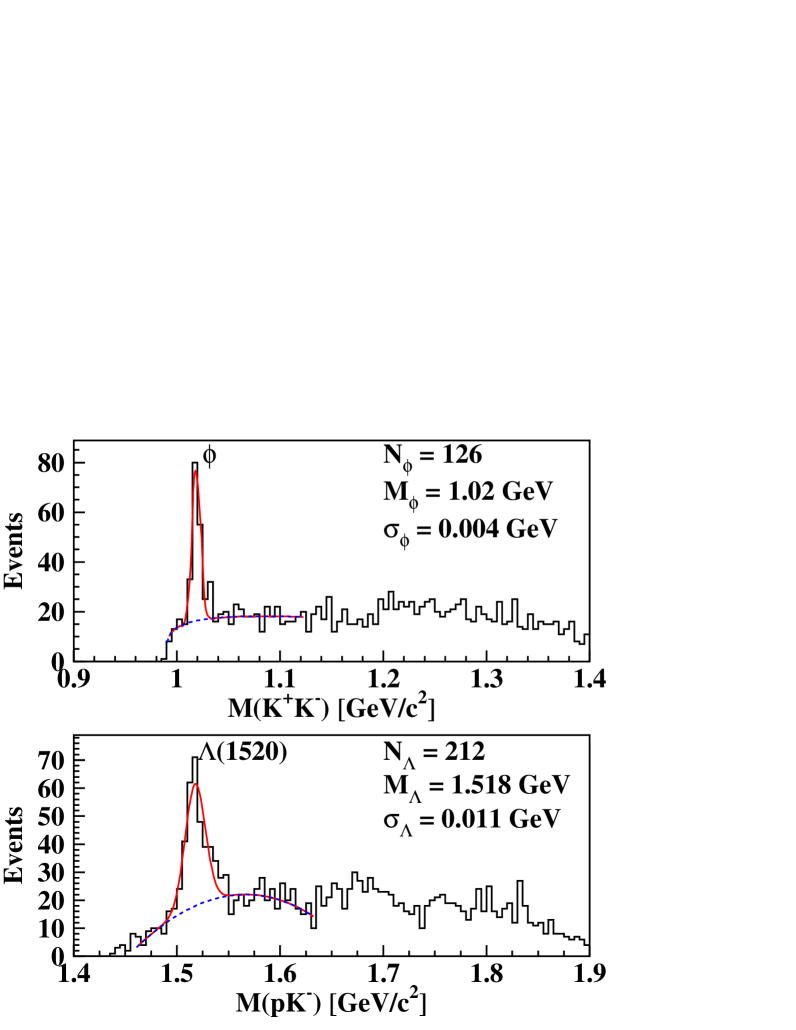
Figure 73: (Top left) The neutron observed in CLAS as missing mass in reaction (36).

Figure 74: (Top right) The $\rm K^{+}K^{-}$ and $\rm pK^{-}$ invariant masses.

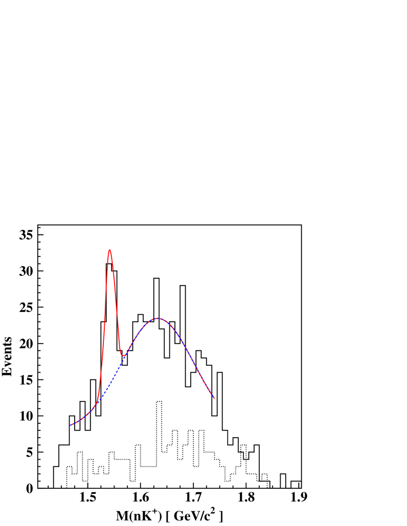
Figure 75: The $\rm nK^{+}$ invariant mass from reaction (36) showing evidence for the $\Theta^{+}(1540)$. All three figures are from $\!{}^{{\bf?}}$.

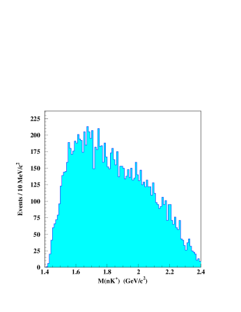
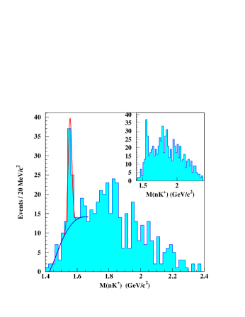
Figure 76: Left: The $nK^{+}$ invariant mass spectrum in the reaction $\gamma p\rightarrow\pi^{+}K^{-}K^{+}(n)$. The neutron was measured from the missing four-momentum. Right: The same invariant mass spectrum with the cut $\cos\theta^{*}_{\pi^{+}}>0.8$ and $\cos\theta^{*}_{K^{+}}<0.6$. $\theta^{*}_{\pi^{+}}$ and $\theta^{*}_{K^{+}}$ are the angles between the $\pi^{+}$ and $K^{+}$ mesons and photon beam in the center-of-mass system. The background function we used in the fit was obtained from the simulation. The inset shows the $nK^{+}$ invariant mass spectrum with only the $\cos\theta^{*}_{\pi^{+}}>0.8$ cut $\!{}^{{\bf?}}$.

The data using H₂ $\!{}^{{\bf?}}$are shown in figure 76. The $\rm nK^{+}$ distribution has a large background; a statistically not very significant peak is present at about 1.55 GeV. The significance of the peak can be improved by selecting events in which the $\pi^{+}$ goes forward, and the $\rm K^{+}$ backward. Both distributions are reproduced in figure 76.

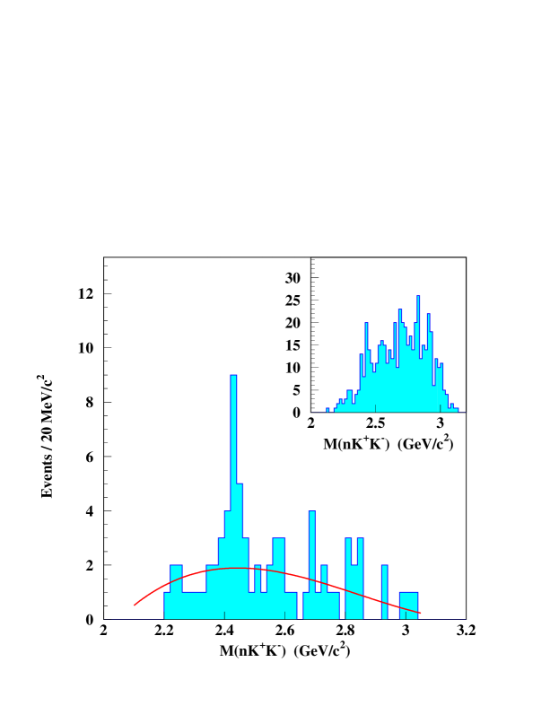
Figure 77: The $nK^{+}K^{-}$ invariant mass spectrum for events having $M(K^{+}n)$ between 1.54 and 1.58 GeV/c². The inset shows the  $nK^{+}K^{-}$ invariant mass spectrum for all events in Figure 76 (left spectrum) $\!{}^{{\bf?}}$.

The energy dependence of the $\Theta^{+}(1540)$ production in figure 77 shows a peculiar pattern: it could be that the $\Theta^{+}(1540)$ is produced via a sequence

$$\rm\gamma p\to N(2430)\pi^{+}\ ,\ N(2430)\to\Theta^{+}(1540)K^{-}\ ,\ {\rm and\ }\Theta^{+}(1540)\to nK^{+}.$$ (38)

The figure shows the $nK^{+}K^{-}$ invariant mass spectrum calculated from the missing mass off the $\pi^{+}$ in the reaction $\gamma p\rightarrow\pi^{+}K^{-}K^{+}(n)$ with cuts $\cos\theta^{*}_{\pi^{+}}>0.8$ and $\cos\theta^{*}_{K^{+}}<0.6$. A peak in this distribution would indicate that the $\Theta^{+}(1540)$ is at least partly produced via reaction chain (38).

The $\Theta^{+}(1540)$ from neutrino–induced reactions

The $\Theta^{+}(1540)$ was also reported from neutrino–induced reactions. Asratyan, Dolgolenko and Kubantsev $\!{}^{{\bf?}}$ scanned data taken with two large bubble chambers at CERN and at Fermilab in the search for the formation of the $\Theta^{+}(1540)$ in collisions of neutrino and antineutrino in the 100 GeV energy range with protons, deuterons and Neon nuclei. A narrow p$\rm K^{0}_{s}$ peak at a mass of $1533\pm 4$ MeV was observed, see figure 78 which is assigned to $\Theta^{+}(1540)$ production (the peak might be a $\Sigma^{+}$ resonance but none is known at this mass).

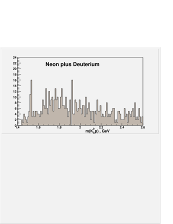
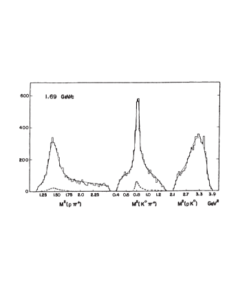
$\Downarrow$

Figure 78: Left: The $\Theta^{+}(1540)$ in $\nu$–induced reactions. Protons and $\rm K^{0}_{s}$ (identified by their $\pi^{+}\pi^{-}$ decay) were produced inclusively in high–energy $\nu$ beams hitting deuterons or Neon nuclei. The $\rm pK^{0}_{s}$ invariant mass distribution peaks at 1.54 GeV $\!{}^{{\bf?}}$. Right: Bubble chamber data on $\rm K^{+}p\to pK^{0}_{s}\pi^{+}$. The fit to the data misses a small enhancement in the $\rm pK^{0}_{s}$ mass distribution marked by $\Downarrow$ which happens to occur at $\sim$1.53 GeV $\!{}^{{\bf?}}$.

The $\Theta^{+}(1540)$ from the archive

It may be worthwhile to note that hints for the $\Theta^{+}$ may have been seen already in 1973 in a CERN experiment to study $\rm K^{+}p\to pK^{0}_{s}\pi^{+}$ inelastic scattering$\!{}^{{\bf?}}$. Mass distributions for the 5000 events are shown in figure 78, right, for a 1.69 GeV/c incident Kaon momentum. On the very right, the $\rm pK^{0}_{s}$ invariant mass distribution shows a low–mass peak which is not accounted for in the fit (which describes the full reaction dynamics). The peak has about 100 events and is seen at 1.53 GeV The 5000 events corresponded to a cross section of 4 mb, hence the $\Theta^{+}$ may have been observed with a cross section of 0.08 mb while the $\Delta(1232)$ is observed with $\sigma\sim 2$ mb, only 25 times stronger.

The Hermes experiment

The Hermes collaboration $\!{}^{{\bf?}}$ searched for the $\Theta^{+}$ in quasi-real photoproduction on deuterium in the $\Theta^{+}\to pK^{0}_{S}\to p\pi^{+}\pi^{-}$ decay chain. The virtual photons originated from the 27.6 GeV (9 to 45 mA) positron beam of the HERA storage ring at DESY. An integrated luminosity of 250 pb^-1 was collected on a longitudinally polarized deuterium gas target. The data shown in figure 79 is summed over two spin orientations.

Selected events contained at least two oppositely charged pions in coincidence with one proton. The event selection included constraints on the event topology to maximize the yield of the $\rm K^{0}_{s}$ peak in the $M_{\pi^{+}\pi^{-}}$ spectrum while minimizing its background. The position of the $\rm K^{0}_{s}$ peak is within 1 MeV of the expected value. To search for the $\Theta^{+}$, events were selected with a $M_{\pi^{+}\pi^{-}}$ invariant mass compatible with the $\rm K_{s}^{0}$ peak. The resulting spectrum of the invariant mass of the $\pi^{+}\pi^{-}p$ system is displayed in figure 79. It is assumed that Pythia describes only the

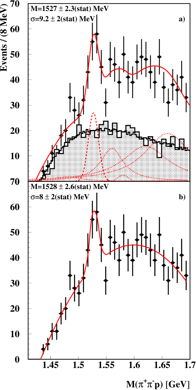
non–resonant background and that low–mass baryon resonances can be added to the non–resonant background. The resulting $\rm pK^{0}_{s}$ spectrum, shown in figure 79, displays a narrow peak at a mass of 1528 MeV. There is no known positively charged strangeness–containing baryon in  this mass region that could account for the observed peak. It is interpreted as further evidence for the $\Theta^{+}(1540)$.

Figure 79: Invariant mass distribution of the $p\pi^{+}\pi^{-}$ system after cuts to optimize the signal–to–background for the $\rm K^{0}_{s}$. The data is represented by dots with statistical error bars. In panel a) the Pythia Monte Carlo simulation is represented by the gray shaded histogram. The fine-binned histogram represents a model based on event mixing and the solid line is the result of the fit taking contributions from known baryon resonances into account, represented by dotted lines. In panel b) a fit to the data of a Gaussian plus a third-order polynomial is shown $\!{}^{{\bf?}}$.

The SVD-2 experiment at Protvino

The SVD-2 spectrometer works in the $70\ GeV$ proton beam of the IHEP accelerator. The beam, defined by microstrip Si-detectors and several dipole and quadrupole magnets, hit an active target (Si-detector and lead foil sandwich); charged particles produced on nuclei were detected in a large–aperture magnetic spectrometer. High–energy $\gamma$’s werde detected in Cherenkov lead glass counters. Events with charged–particle multiplicity five or less were selected to reduce the combinatorial background. The following cuts were made: a $\rm K^{0}_{s}$ was required, $\Lambda^{0}$’s were excluded, the $\rm pK^{0}_{s}$-system was required to be produced in forward direction. A cut on the $\rm K^{0}_{s}$ momentum $\rm P_{K^{0}_{s}}\leq~{}P_{p}$ improved the signal to background ratio.

The resulting $\rm K^{0}_{s}$ invariant mass spectrum  $\!{}^{{\bf?}}$ exhibits a peak interpreted as further evidence for the existence of the $\Theta^{+}(1540)$. The mass was determined to $M=1526\pm 3(stat.)\pm 3(syst.)$ MeV/c², the width is compatible with the experimental resolution, thus $\Gamma<24$ MeV/c². A statistical significance of $5.6~{}\sigma$ is estimated.

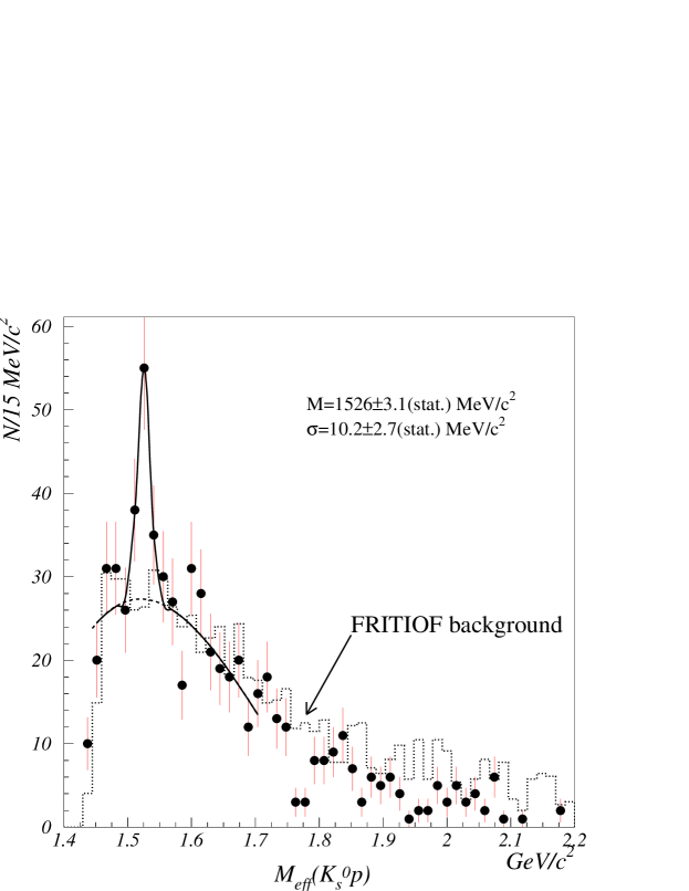
Figure 80: The $(pK^{0}_{s})$ invariant mass spectrum in the reaction $\!{}^{{\bf?}}$ $pA\rightarrow pK^{0}_{s}+X$. The dashed histogram represents background obtained from simulations.

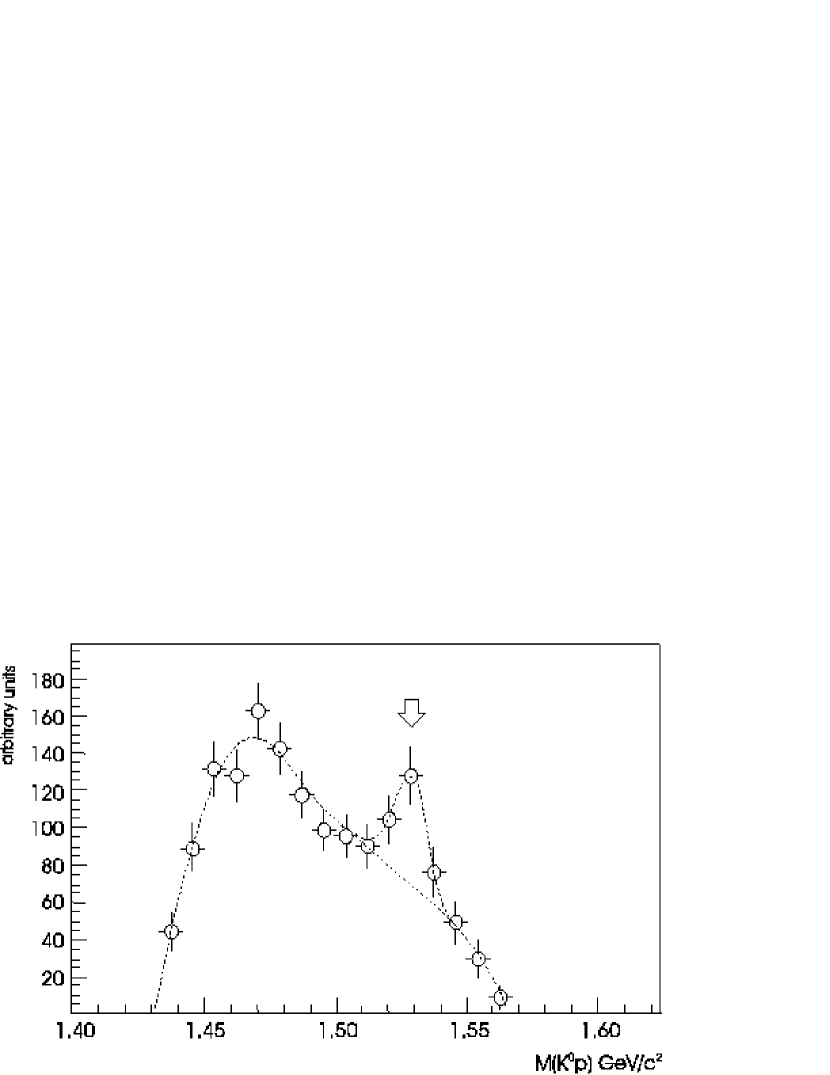
Figure 81: The $\rm pK^{0}_{s}$ invariant mass distribution from the reaction $\rm pp\to\Sigma^{+}K^{0}_{s}p$ at COSY $\!{}^{{\bf?}}$.

The TOF experiment at COSY

At the Cooler Synchroton (COSY) at Jülich, the reaction $\rm pp\to\Sigma^{+}K^{0}_{s}p$ was studied $\!{}^{{\bf?}}$ in a proton beam of 2.95 GeV/c momentum impinging on a liquid H₂ target of 4 mm length. Charged particles were tracked using a double–sided silicon microstrip detector close to the target and scintillation fiber hodoscopes. There is no magnetic field; momenta were determined from the event geometry. The $\Sigma^{+}$ was identified from a kink in the track due to $\rm\Sigma^{+}\to p\pi^{0}$ decays, the $\rm K^{0}_{s}$ by its decay to $\pi^{+}\pi^{-}$. In the $\rm pK^{0}_{s}$ invariant mass distribution a peak shown in figure 81 is observed which is fit to $1530\pm 5$ MeV. The width (FWHM) $18\pm 4$ MeV is compatible with the instrumental resolution and is quoted as upper limit. The statistical significance is 3.7.

Yerevan

A group at Yerevan $\!{}^{{\bf?}}$ reported a search for the $\Theta^{+}$ in a 2m propane bubble chamber by scattering 10 GeV/c protons off $\rm C_{3}H_{8}$. The $\rm pK^{0}_{s}$ invariant mass spectrum shows resonant structures with $\rm M_{K_{s}^{0}p}$=1545.1$\pm$12.0, 1612.5$\pm$10.0, 1821.0$\pm$11.0 MeV/$c^{2}$ and $\rm\Gamma_{K_{s}^{0}p}$= 16.3$\pm$3.6, 16.1$\pm$4.1, 28.0$\pm$9.4 MeV/$c^{2}$, respectively. Protons were se lected to have large or small momenta. The statistical significance of these peaks were estimated to 5.5$\sigma$,4.6$\sigma$ and 6.0$\sigma$, respectively.

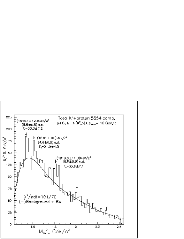
Figure 82: The effective $pK^{0}_{s}$ mass distribution for protons with momenta between $0.35\leq p\leq 0.9$ GeV/c² or $p\geq 1.7GeV/c^{2}$. For momenta between $0.9\leq p\leq 1.7$ GeV/c² there is no significant signal and the date is excluded. The curve is the experimental background from an mixing method taken in the form of six-order polynomial $\!{}^{{\bf?}}$.

The ZEUS experiment at HERA

The ZEUS experiment studied the $\rm K^{0}_{s}p$ and $\rm K^{0}_{s}\bar{p}$ invariant mass spectra in inclusive deep inelastic $ep$ scattering for a large range in the photon virtuality $\!{}^{{\bf?}}$. For $Q^{2}\geq 10$ GeV² a peak is seen around 1520 MeV. The peak position is $1521.5\pm 1.5({\rm stat.})^{+2.8}_{-1.7}({\rm syst.})$ MeV; the Gaussian width corresponds to a full width at half maximum of 16 MeV we take as upper limit of the natural width. The statistical significance is about 4.6$\sigma$. The fit suggests an additional $\Sigma(1465)$ bump (possibly identical with a $\Sigma(1480)$ bump $\!{}^{{\bf?}}$ reported from $\rm K^{-}p\to K^{0}\pi^{-}p$ at 4.2 GeV). The $\Theta^{+}(1540)$ evidence reduces to 3$\sigma$ when the $\Sigma(1465)$ bump is excluded from the fit.

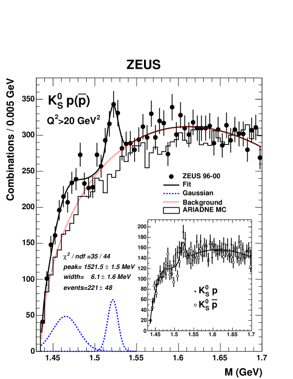
Figure 83: Invariant-mass spectrum for the $\rm K^{0}_{s}p$ and $\rm K^{0}_{s}\bar{p}$ channel for $Q^{2}>20$ GeV² $\!{}^{{\bf?}}$. The solid line is the result of a fit to the data using a three-parameter background function plus two Gaussians (see text). The dashed lines show the Gaussian components and the dotted line the background according to this fit. The histogram shows the prediction of the Ariadne MC simulation normalised to the data in the mass region above $1650$ MeV. The inset shows the $\rm K^{0}_{s}p$(open circles) and the $\rm K^{0}_{s}\bar{p}$ (black dots) candidates separately, compared to the result of the fit to the combined sample.

The results provide further evidence for the existence of a narrow baryon resonance consistent with the predicted $\Theta^{+}$ pentaquark state with a mass close to $1530$ MeV and a width of less than $15$ MeV. In the $\Theta^{+}$ interpretation, the signal observed in the $\rm K^{0}_{s}\bar{p}$ channel corresponds to first evidence for an antipentaquark with a quark content of $\bar{u}\bar{u}\bar{d}\bar{d}s$. The results, obtained at high energies, constitute first evidence for the production of such a state in a kinematic region where hadron production is dominated by fragmentation.

Search for the $\Theta^{+}(1540)$ at HERA-B

Knöpfle, Zavertyaev and Zivko $\!{}^{{\bf?}}$ reported a search for pentaquarks in HERA-B data taken with a minimum bias trigger (more than 200 million events). HERA-B is a fixed target experiment at the 920 GeV proton storage ring of DESY hitting a carbon, titanium or tungsten target. The forward magnetic spectrometer has large acceptance, high-resolution vertexing and tracking and good particle identification. In the $\rm pK^{-}$ invariant mass distribution a clear $\Lambda(1520)$ is seen, but there is no sign of the $\Theta^{+}(1540)$.

Figure 84: The pK${}^{0}_{s}$ invariant mass distributions $\!{}^{{\bf?}}$: a) data from the p+C collisions with background (continuous line) determined from event mixing; b) as a) but with the background subtracted; c) as a) but requiring a track multiplicity of $<10$. d) data from all targets C, Ti, W requiring a track multiplicity of $<20$ and a $\Lambda$ particle in the event. Arrows mark the mass of 1540 MeV/c² .

Search for the $\Theta^{+}(1540)$ in charmonium decays

The BES collaboration serached for the $\Theta^{+}(1540)$ in J/$\psi$ and $\psi(2S)$ decays into different charge combinations of the $\rm N\bar{N}K\rm\bar{K}$ final state $\!{}^{{\bf?}}$. The reactions are observed with branching ratios in the order of $10^{-4}$ and with no evidence for the $\Theta^{+}(1540)$ at the $10^{-5}$ level.

The $\Xi^{--}$ from NA49

The NA49 collaboration reported evidence for another exotic baryon resonance with strangeness S=-2 and charge Q=-2 $\!{}^{{\bf?}}$. A state with these quantum numbers cannot be constructed from three quarks; the minimum quark model configuration is $ddssu$. It is a pentaquark called $\Xi^{--}$.

The $\Xi^{--}$ was observed in fixed-target proton-proton collisions at the Super Proton Synchrotron (SPS) at CERN. The center-of-mass energy of these collisions was 17.2 GeV, far above the threshold for pentaquark production. The NA49 detector consists of large acceptance Time Projection Chambers (TPCs) providing tracking for charged particles produced from primary and secondary vertices. Particles are identified by specific energy loss (dE/dx) in the TPCs.

In a first step, $\Lambda$’s were identified from the invariant mass spectrum of $p\pi^{-}$ pairs originating from the same vertex. $\Lambda$ candidates were then combined with $\pi^{-}$ to form $\Xi^{-}$ candidates. Similarly, both mass distributions were constructed for $\bar{p}\pi^{+}$ and $\bar{\Lambda}\pi^{+}$ (see Figure 85). Finally, the

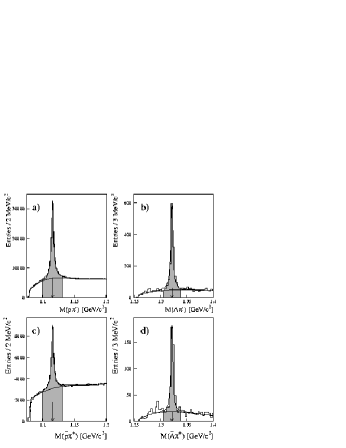
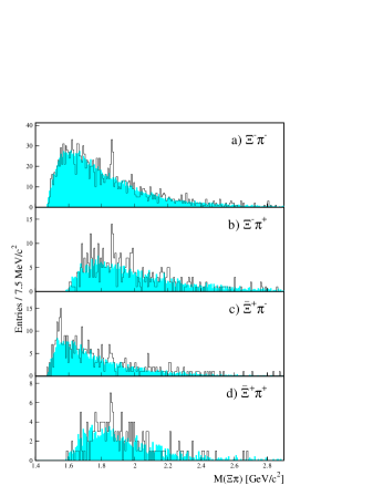
Figure 85: NA49 invariant mass distributions: $\Lambda=p\pi^{-}$, $\Xi^{-}=\Lambda\pi^{-}$ (left) $\Xi(1862)=\Xi^{-}\pi$ (right), and charge conjugated reactions $\!{}^{{\bf?}}$.

$\Xi^{--}$ was searched for in the invariant mass spectrum of the $\Xi^{-}$ ($\bar{\Xi}^{+}$) candidates with $\pi^{-}$ ($\pi^{+}$) tracks originating from the primary vertex.

A peak was seen with a mass of $1862\pm 2$ MeV and a width below the detector resolution of 18 MeV. At the same mass NA49 also observed a peak in the $\Xi^{-}\pi^{+}$ spectrum, which could be a candidate for a neutral isospin-partner of the $\Xi^{--}$. The corresponding antibaryon spectra for both states also show enhancements at the same mass. The four mass spectra are shown in figure 85.

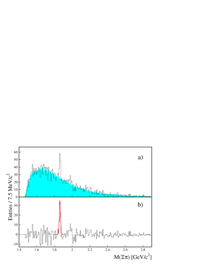
Figure 86: The final $\Xi\pi$ invariant mass spectrum without and with background subtraction. The four spectra shown individually in 85 are added $\!{}^{{\bf?}}$.

Search for the $\Xi^{--}(1862)$ at HERA-B

The HERA-B collabration also reported $\!{}^{{\bf?}}$ a search for the $\Xi(1862)$ in the doubly-charged $\Xi^{-}\pi^{-}$ + c.c. and in the neutral $\Xi^{-}\pi^{+}$ + c.c. channels. $\Xi$ candidates with a mass of $\pm 10$ MeV/c² of the PDG mass were accepted.

Figure 87: The $\Xi\pi$ invariant mass distributions obtained with all targets C, Ti, and W in indicated decay channels $\!{}^{{\bf?}}$. Continuous lines show the background from event mixing. Arrows mark the mass of 1862 MeV/c² .

Figure 87 shows the corresponding invariant mass spectra and the backgrounds determined by event mixing. In the neutral decay channels, (Figure 87a), the $\Xi(1530)^{0}$ resonance shows up with a prominent signal, and there is a possible weak evidence for known higher $\Xi^{*}$ resonances. In the doubly-charged channels (Figure 87b), the background follows very well the data. There is no evidence for a narrow signal at around 1862 MeV/c². $\Xi^{--}(1862)$ production is reduced compared to $\Xi(1530)^{0}$ production by mor than one order of magnitude.

A charming pentaquark

Very recently the H1 collaboration reported a narrow baryon resonance containing a $\bar{c}$–quark $\!{}^{{\bf?}}$. It is observed in inelastic electron-proton collisions at centre-of-mass energies of $300\ {\rm GeV}$ and $320\ {\rm GeV}$ at HERA in the $D^{*\,-}p$ invariant mass spectrum, or as an antibaryon in the $D^{*\,+}\bar{p}$ mass distribution. The final data is shown in figure 88. The resonance has a mass of $3099\pm 3\ {\rm(stat.)}\ \pm 5\ {\rm(syst.)}\ {\rm MeV}$ and a measured Gaussian width of $12\pm 3\ {\rm(stat.)}\ {\rm MeV}$, which is compatible with the experimental resolution. The resonance is interpreted as an anti-charmed baryon with a minimal constituent quark composition of $uudd\bar{c}$ together with the charge conjugate.

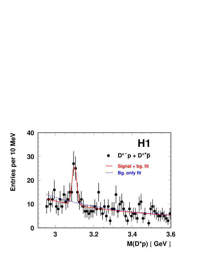
Figure 88: $M(D^{*}p)$ distribution from opposite-charge $D^{*}p$ combinations in deep inelastic scattering of electrons off protons $\!{}^{{\bf?}}$. The solid line represents a fit with a Gaussian peak plus a two–parameter background, the dashed line a fit background only.

Pentaquark summary

Table 27 collects masses, width, number of events and statistical significance of pentaquark observations. There are 11 data points, and at a first glance the existence of the $\Theta^{+}(1540)$ seems to be established beyond any reasonable doubt.

In some papers the statistical evidence is calculated as $\sigma=N/\sqrt{B}$ where $N$ is the number of signal events and $B$ the number of background events. In the limit $B\to 0$, the evidence becomes extremely large and the formula must be wrong. Therefore the statistical evidence has been estimated from the published histograms. The number of events in the signal region is $N+B$, in side band regions (covering the same mass interval) it is $B$, error propagation gives $\sigma=N/\sqrt{(N+2B)}$. Recalculated statistical evidences are denoted by a $\sim$ symbol in table 27. There is only a very small probability that all these measurements are statistical fluctuations.

Now we turn to a discussion of the mass values. The systematic uncertainties of the DIANA and $\nu$–induced measurements were taken to be $\pm 3$ MeV as suggested in $\!{}^{{\bf?}}$. The weighted average of the masses observed in all experiments is $1532.4\pm 1.4$ MeV. In evaluating this average mass value, the quadratic sum of the statistical and systematic uncertainties of all measurements are taken into account. The sum of $\chi^{2}$’s for all data is 38. Hence the probability that all these measurements have observed the same object is also rather small and a scaled mass error $\pm 2.7$ MeV is mor realistic.

Table 27: Summary of measurements of pentaquarks. The systematic errors given in parentheses are not quoted in the papers but were estimated to be small.

Mass	Width	$\rm N_{event}$	Statist.	Reaction	Experiment
(MeV)	(MeV)		signif.
$\Theta^{+}(1540)$
$1540\pm 10\pm 5$	$<25$	$19\pm 2.8$	$\sim 2.7\sigma$	$\rm\gamma C\to C^{\prime}K^{+}K^{-}$	LEPS
$1539\pm 2\pm 2$	$<9$	$29$	$\sim 3.0\sigma$	$\rm\gamma p\to nK^{+}K^{0}_{s}$	DIANA
$1542\pm 2\pm 5$	$<21$	$43$	$\sim 3.5\sigma$	$\rm\gamma d\to pnK^{+}K^{-}$	CLAS
$1540\pm 4(\pm 3)$	$<25$	$63\pm 13$	$4.8\sigma$	$\rm\gamma p\to nK^{+}K^{0}_{s}$	SAPHIR
$1533\pm 5(\pm 3)$	$<20$	$27$	$\sim 4.0\sigma$	$\nu$–induced	CERN, FNAL
$1555\pm 1\pm 10$	$<26$	$41$	$\sim 4.0\sigma$	$\rm\gamma p\to nK^{+}K^{-}\pi^{+}$	CLAS
$1528\pm 4$	$<19$	$\sim 60$	$\sim 4\sigma$	$\gamma^{*}$–induced	HERMES
$1526\pm 3\pm 3$	$<24$	$50$	$3.5\sigma$	p-p reaction	SVD-2
$1530\pm 5$	$<18$		$3.7\sigma$	p-p reaction	COSY
$1545\pm 12$	$<35$	$\sim 100$	$\sim 4\sigma$	p-A reaction	YEREVAN
$1521.5\pm 1.5^{+2.8}_{-1.7}$	$<6$	$221$	$4.6\sigma$	Fragmentation	ZEUS
$\Xi(1862)$
1862	$<21$		$4.6\sigma$	$\nu$–induced	NA49
$\Theta_{c}(3099)$
$3099\pm 3\pm 5$			$5.4\sigma$	$\gamma^{*}$–induced	HERA

A statistical analysis is not the only criterion for judging observations. In spite of the fact that physics is an exact science, there might also be some ’personal bias’. There might be a tendency to increase the error if the measured mass seems to be ’wrong’. Hence the probability of consistent mass values could be even smaller. Further, in the data selection cuts are applied some of which are tuned to optimize the signal; these cuts enhance the statistical evidence and the reported evidence becomes too high.

We remind the reader that a long time ago there was striking evidence that the $a_{2}(1320)$ was split into two mesons at slightly different masses $\!{}^{{\bf?}}$. The so–called $S(1936)$ meson was seen in several experiments and interpreted as $\rm N\bar{N}$ bound state. It was proven not to exist when high-statistics data became available at LEAR (see, e.g. $\!{}^{{\bf?}}$). Also, the production characteristics are sometimes different, in particular the ratio of $\Lambda(1520)$ and $\Theta^{+}(1540)$, even though the reactions are similar or even identical. (However, the data is not acceptance–corrected, and the detection efficiencies for $\Lambda(1520)$ and $\Theta^{+}(1540)$ can be different.) Experiments not observing a signal have more difficulties to publish upper limits than experiments reporting positive evidence have. First data with negative evidence is now published but there are rumors also from other experiments finding no $\Theta^{+}(1540)$, $\Xi(1862)$ or $\Theta^{+}_{c}(3099)\pm 3\pm 5$.

Another important aspect was underlined by A. Dzierba and collaborators $\!{}^{{\bf?}}$. In the reaction $\rm\gamma N\to NK\bar{K}$ one should consider the full three–particle dynamics. Not only can $\rm NK$ or $\rm N\bar{K}$ resonances be produced but also $\rm K\bar{K}$ resonances.

The full dynamics can be studied in the Dalitz plot. In photoproduction with a continuous photon energy spectrum, the Dalitz plot does not have fixed boundaries. This is made visible in figure 90. The $a_{2}(1320)$ and $f_{2}(1270)$, which can decay into $\rm K\bar{K}$, are particularly important since they have, as tensor mesons, a non–uniform decay angular distribution as can be seen in figure 90.

Figure 89: Boundaries of the $m_{KK}^{2}$ versus $m_{KN}^{2}$ Dalitz plot for three different values of $w$, the energy available to the $\rm K\bar{K}N$ system, 2.1, 2.4 and 2.6 GeV. For the CLAS data $\!{}^{{\bf?}}$ the observed distribution in $w$ rises from 2.1 GeV, peaks at 2.4 and falls to zero near 2.6 GeV. Horizontal lines denote the region spanned by the $f_{2}$ and $a_{2}$ mesons defined by their half-widths and the region of the $\rho_{3}$ starting with its central mass less its half-width. The vertical line denotes the square of the $\Theta$ mass $\!{}^{{\bf?}}$.

Figure 90: The $m_{KN}$ mass distribution for a fixed   $m_{KKN}$ mass of 2.6 GeV/$c^{2}$. The two-peaked curve assumes   $m_{KK}=m(a_{2})$ with $|Y^{\pm 1}_{2}|^{2}$ and and the three-peaked curve assumes $m_{KK}=m(\rho_{3})-\Gamma_{\rho}/2$ with $|Y^{\pm 1}_{3}|^{2}$ for the decay angular distribution $\!{}^{{\bf?}}$.

These decay angular distributions must be integrated over the photon energy spectrum; the resulting spectrum is compared to the CLAS data$\!{}^{{\bf?}}$. You should compare figure 91 with figure 36 to see the extent to which the eye is guided by a line connecting data points. Figure 75 and figure 91 show the same data ! Even though the $\Theta^{+}(1540)$ is observed in rather different final states and not all peaks can be explained by reflections, the analysis points out very clearly the traps into which experimenter may fall.

A second weak point was discussed by Zavertyaev $\!{}^{{\bf?}}$. He simulates the DIANA experiment but his word of caution may also apply to other experiments. Charged particles from secondary $\rm K^{0}_{s}$ or $\Lambda$ decays may cause spurious peaks when they are misidentified. Due to the limited range of the selected Kaons, the phase space distribution peaks at about the observed $\rm pK^{0}_{s}$ invariant mass. Thus small statistical fluctuation may mimique a narrow signal.

Clearly the aim of further studies must be to increase the statistics considerably, in order to allow for more systematic studies. Finally, one needs to observe the natural width experimentally and to deduce a phase motion. Of course, spin and parity have to be determined. This will, if successful, also provide final support to establish the $\Theta^{+}(1540)$ as the first baryon resonance with exotic quantum numbers.

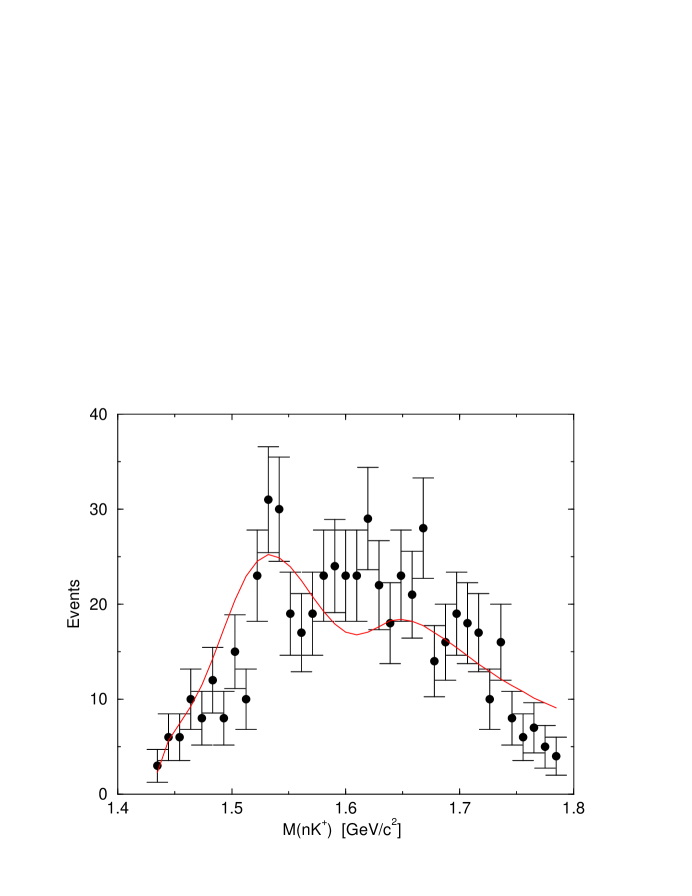
Figure 91: The calculated (solid line) $m_{KN}$ distribution $\!{}^{{\bf?}}$, compared with the data $\!{}^{{\bf?}}$.

Even though there are reasons one should still be cautious in accepting the $\Theta^{+}(1540)$ as an established particle, a short and very incomplete survey will be given on how to interprete the $\Theta^{+}(1540)$.

The $\Theta^{+}(1540)$ was predicted as a narrow resonance with width less than 15 MeV and at a mass of 1530 MeV in the chiral soliton model $\!{}^{{\bf?}}$. (Jaffe $\!{}^{{\bf?}}$ claimed that the predicted width should rather be 30 MeV.) This is very close to the observed $\Theta^{+}(1540)$ mass; this agreement was certainly (and still is) an important stimulus for the excitement with which the $\Theta^{+}(1540)$ is discussed. The same paper predicts the $\Xi^{--}$ at 2070 MeV, far from the observed 1862 MeV. The mass difference between a $\Xi^{--}(1862)$ and the $\Theta^{+}(1540)$ is certainly closer to what we expect from the quark model for one $n$–quark replaced by a $s$–quark. The chiral soliton model needs to be readjusted $\!{}^{{\bf?}}$ because of a change in the value of the pion–nucleon $\sigma$ term, $\rm\sigma_{\pi N}$. In any case, the chiral soliton model predicts the $\Theta^{+}(1540)$ to have $J^{P}=1/2^{+}$ even though negative parity might not be excluded $\!{}^{{\bf?}}$.

A rapidly increasing number of papers investigates the possibilities of further pentaquark studies, the expected masses within different models and the consequences of pentaquarks for models. It is far beyond the scope of this paper to review them here. Only a few selected topics reflecting the limits of the author will be mentioned.

A system of four quarks and an antiquark all in an S–wave leads to a negative parity. Quark models of the $\Theta^{+}(1540)$. predict therefore naturally $P=-1$. A natural explanation of the $\Theta^{+}(1540)$ would be a $\rm NK$ resonance bound by nuclear interactions. However, such bound states are expected to be very broad. Alternatively, one may ask if quark models support five–quark configurations $\!{}^{{\bf?}}$. Capstick, Page and Roberts $\!{}^{{\bf?}}$ interpret the $\Theta^{+}(1540)$ as an isotensor resonance which is narrow as it requires isospin violation for its decay. The model predicts charged partners unobserved with the expected yields. So this solution seems unlikely. Strong correlations between the quarks in a pentaquark may lead to an inversion of states and to the prediction of positive parity for the $\Theta^{+}(1540)$. Such models are proposed by Karliner and Lipkin $\!{}^{{\bf?},{\bf?},{\bf?}}$ and by Jaffe and Wilczek $\!{}^{{\bf?}}$. Lattice calculations also report evidence for the $\Theta^{+}(1540)$ and negative parity as preferred solution $\!{}^{{\bf?}}$.

6 Interpretation

This is a write–up of a lecture course. I will given a very personal interpretation of the status of the field. Most physicists working in hadron physics do not share my view (but they did not give these lectures). To make the view clear, I will not mention the many ’buts’. What I present is not a theory, not even a model. However, I believe that present–day models aiming at understanding strong interactions in the confinement region partly use the wrong degrees of freedom, e.g. one–gluon exchange between constituent quarks, gluonic flux tubes without sea quarks, constituent quarks with masses which do not change (apart from an relativistic mass increase) when a hadron is excited, and gluons as constituent parts of hadrons, glueballs and hybrids. Even though I have no model to present, I will outline how strong interactions might possibly work. In the best case you may remember some of the ideas in the course of your own work; maybe these ideas are better adapted to your findings and will encourage you to continue and not be threatened away, since you feel you might be off-side. I start the discussion with ideas about what might be a constituent quark. The discussion will provide a frame allowing us to approach various topics from a similar point of view.

6.1 Constituent quarks

Quarks do not move freely within hadrons; there is a rapid spin and flavor exchange, e.g. due to instanton–induced interactions. Due to the strong color charge, the vacuum is polarized and the color charge is (anti–)screened. The mass of the proton is not the sum of 3 current quark masses. The largest fraction is due to the field energy of the polarized Dirac sea. If forces act upon a quark and an antiquark and their separation increases, the region where the Dirac sea is polarized increases, the quark plus field energy increases, the constituent quark mass increases.

Color and flavor exchange

Color exchange is usually thought of as a fast process enforcing the overall symmetry of the wave function. Consider a $\Delta^{++}_{7/2}(1950)$. Isospin is 3/2 (three up quarks), the leading internal orbital angular momentum is $L=2$, the spin $S=3/2$. The antisymmetry of the wave function with respect to the exchange of any pair of quarks is guaranteed by color; each of the three quarks may have color blue, red or green. To ensure the symmetry properties of wave function, there is a fast exchange of any pair of quarks, or properties of quarks are changed, e.g. two quarks may change their color by gluon exchange. At the time a proton is excited to the $\Delta^{++}_{7/2}(1950)$, a colored quark is struck. The large excitation energy is due to the separation of the color sources in space, in the same way the excitation of a hydrogen atom leads to a separation of the electric charges. The struck quark and the two quarks in the remaining diquark still undergo rapid exchanges. Can we ask which process is faster, quark exchange or color exchange ? Can we measure the frequencies of color and spin/flavor exchange ?

In principle yes, even though I do not know how. The forces leading to the exchange of quarks cannot be controlled experimentally, but there is no quantum mechanical argument against such a measurement.

Gluon exchange is likely a slow process. I assume that the strong color-forces polarize the quark and gluon condensates of the QCD vacuum. The current quark plus its polarization cloud forms what I call a constituent quark of defined color. Color exchange is screened by the polarization cloud. When a gluon is emitted it is re-absorbed in the polarization cloud. Color propagates only stochastically from one color source to the next source within a polarization cluster. Globally a constituent quark keeps its color for a finite time which may be longer than the lifetime for flavor exchange. The matrix element governing color exchange is not known; we estimate it to be on the order of $\Lambda_{\rm QCD}$ (200 MeV).

In contrast to color exchange there is a fast flavor exchange. Flavor exchange is not shielded by the polarized condensates; flavor propagates freely in the QCD vacuum. Flavor exchange is possible via long-range meson-exchange or by instanton–induced interactions at the surface of two neighboring colored constituent quarks. Flavor exchange acts at a time scale given by chiral symmetry breaking, by $\Lambda_{\chi}$ (1 GeV). In this picture confinement originates from Pomeron-exchange-like forces transmitted by the polarization of the vacuum condensates.

Regge trajectories

This picture suggests that the largest contribution to the mass of a hadron comes from the mass density of the polarization cloud and the hadronic volume. This idea can be tested in a string model of quark-diquark interactions. We assume that the polarization cloud between quarks and diquarks is concentrated in a rotating flux tube or a rotating string with a homogeneous mass density. The length of the flux tube is $2r_{0}$, its transverse radius $R$. The velocity at the ends may be the velocity of light. Then the total mass of the string is given by $\!{}^{{\bf?}}$

$$Mc^{2}=2\int_{0}^{r_{0}}\frac{kdr}{\sqrt{1-v^{2}/c^{2}}}=kr_{0}\pi$$ (39)

and the angular momentum by

$$L=\frac{2}{\hbar c^{2}}\int_{0}^{r_{0}}\frac{krvdr}{\sqrt{1-v^{2}/c^{2}}}=\frac{kr_{0}^{2}\pi}{2\hbar c}$$ (40)

The orbital angular momentum is proportional to

$$L=\frac{1}{2\pi k\hbar c}M^{2}.$$ (41)

This is the linear relation between $L$ and $M^{2}$ as expected from Regge theory.

From the slope in Fig. 59 we find $k=0.2$ GeV² The volume of the flux tube is 2$\rm\pi R^{2}r_{0}$, the mass density

$$\rho=\frac{k}{2R^{2}c^{2}}.$$ (42)

We now assume that the mass density in the $\Delta(1232)$ is the same as the one in the flux tube. We thus relate

$$\frac{4}{3}\pi R^{3}\cdot\rho=M_{\Delta(1232)}$$ (43)

which gives a radius of the polarization cloud of the $\Delta(1232)$ of 0.6 fm (and 0.37 fm for the $\rho$). This is not unreasonable, even though smaller than the RMS charge radius of the proton. However, an additional pion cloud would increase the charge radius.

The size of excited nucleons

We now calculate the radius of a highly excited baryon, of the $\Delta_{15/2^{+}}(2950)$. We find a radius of

$$r_{0}\left(\Delta_{15/2^{+}}(2950)\right)=4\,{\rm fm}.$$ (44)

According to the Nambu model the excited quark and the diquark in the $\Delta_{15/2^{+}}(2950)$ are separated by 8 fm !

Consequences of the colored-constituent-quark concept

The assumption that constituent quarks have a defined color, and that color exchange is shielded by the polarization cloud offers a new interpretation for a large number of phenomena which are partly not understood yet.

Confinement:

When two quarks are separated, the volume in which the QCD vacuum is polarized increases with the quark-quark separation. The net color charge does not change, hence the energy stored in the polarized condensates increases linearly. The confinement potential is a linear function of the quark separation.

Structure functions:

The polarization clouds surrounding the current quarks are of course seen in deep inelastic scattering, the quarks directly and the gluons through their contribution to the total momentum.

The spin crisis:

It was a surprising discovery that the proton spin is not carried by quarks. The success of the naive quark model in the prediction of the ratios of magnetic moments of octet baryons seemed to be a solid basis for the assumption that the spin of the proton should be carried by its 3 valence quarks. But this naive expectation fails; the contribution of all quark- and antiquark-spins to the proton spin is rather small. A large fraction of the proton spin must be carried by the intrinsic orbital angular momenta of quarks or by orbital or spin contributions of gluons. We assume that the magnetic moment of the spin induces polarization into the condensates. The polarized gluon condensates provide a gluonic contribution to the proton spin, the quark condensate a spin and orbital angular momentum contribution. Orbital angular momenta of quarks enter because the quarks in the condensate are pairwise in the ${}^{3}{\rm P}_{0}$ state. The orientation defined by the direction of the current-quark spin may induce internal currents which contribute to the magnetic moment.

An analogy can be found in superconductivity. If a magnetic moment is implanted into a superconducting material, the Cooper pairs will be polarized and the currents adjust to take over part of the magnetic moment of the alien element.

The ${}^{3}{\bf\rm P}_{0}$ model:

A further example for the usefulness of the concept proposed here is the ${}^{3}{\rm P}_{0}$ model for meson and baryon decays. According to this model the quantum numbers of a $\rm q\bar{q}$ pair, created in a decay process, have the quantum numbers of the vacuum. These quantum numbers are preserved, when a $\rm q\bar{q}$ pair from the condensate is shifted to the mass shell.

Baryon resonances in nuclei:

Baryons can be excited inside of a nucleus. The total photo–absorption cross section of light nuclei shows s strong peak at the mass of the $\Delta(1232)$. Obviously, the $\Delta(1232)$ can be excited and is long–lived; the $\Delta(1232)$ survives the nuclear environment. The total cross section does not show, however, any peak for the $N(1520)D_{13}$. Why does the $\Delta(1232)$ survive but not the $N(1520)D_{13}$ ? As free particles they have similar widths. The width of the $\Delta(1232)$ remains practically unchanged in a nucleus and the $N(1520)D_{13}$ becomes so broad that it disappears completely. The reason for the disappearance of the $N(1520)D_{13}$ may be a sizable coupling to N$\rho$. In nuclear matter, the $\rho$ may become very broad and the increase in phase space could be responsible for the extremely short life time of the $N(1520)D_{13}$. This could be calculated. A further effect is the momentum of the struck nucleon leading to a Doppler shift and broadening of the $N(1520)D_{13}$. The latter effect could be avoided by recoilless production of the resonance. Within the view suggested here, there is no surprise. The $\Delta(1232)$ has $L=0$ and is a compact object. The $N(1520)D_{13}$ is extended over a string of more than 3 fm and does not fit into the empty regions of the nucleus.

6.2 Quark–quark interactions

With QCD being “the theory of strong interactions”, one might be tempted to assume that one gluon exchange is the dominant mechanism with which forces between quarks or quarks and antiquarks are mediated. We know that with increasing distance, at small momentum transfers, the strong interaction coupling constant $\alpha_{s}$ increases. Thus the expansion series in powers of $\alpha_{s}$ may become ill–behaved or even divergent but this effect can possibly be taken into account by defining an effective $\alpha_{s}(eff)$ with a value adapted to reproduce experimental data by dynamical quark models in first–oder-perturbation theory. This approach neglects the important role of the QCD vacuum, of quark and gluon condensates, of the role of instantons, and of QCD fields of non–trivial topological configurations. We may therefore ask if the dominant contribution to quark–quark interactions in the domain of the confinement forces are given by direct interactions between the quarks and antiquarks, or if the interactions are mostly indirect, mediated by changes of the QCD vacuum due to the presence of a quark; the polarized QCD vacuum then transmits the interaction.

Do we have evidence for one–gluon exchange in spectroscopy ?

The bottonium family of states and, to a lesser extend also the charmonium family, can be described by a confinement potential plus one–gluon exchange. The confinement potential dominates the interaction and still has the same strength as the Coulomb part at a distance of about 0.25 fm. Gluon exchange is a short range phenomenon, effective for typical distances of up to 0.25 fm. At larger distances there is no free gluon wave propagating through the vacuum and transmitting the force. At distances above 0.25 fm collective phenomena become decisive ! Hence we cannot expect that an extrapolation of one–gluon exchange to light mesons and baryons is meaningful.

Models based on one–gluon exchange do result in a rather good description of the meson and baryon mass spectra even though the quantitative agreement is better for the model using instanton–induced interactions. More convincing are the following two observations. First, models based on one–gluon exchange suppress spin–orbit interactions ’by hand’. This is called the spin–orbit problem. The excuse is that the calculation of the mass spectra is non–relativistic. Thus the Thomas precession is neglected which compensated at least partly the effect of spin–orbit forces due to one–gluon exchange. This is unsatisfactory, and wrong. In a full relativistic treatment, confinement plus one–gluon exchange result in large spin–orbit forces $\!{}^{{\bf?}}$, in contrast to the conjecture that there might be exact cancellation of spin–orbit interactions and the Thomas precession.

Instanton–induced forces

The spectra of light mesons and light baryons can both be described reasonably well when instanton–induced forces are used to describe residual interactions (i.e. the interactions which remain once confinement is taken care of by a confinement potential). Instanton–induced interactions were introduced to solve the so–called UA(1) problem, the large $\eta^{\prime}$ mass. And these interactions provide for a plausible interpretation of the scalar mass spectrum, too. Personally, I consider the systematics leading to figure 60 to provide the most direct evidence for the role of instanton–induced interactions in spectroscopy.

Do glueballs and hybrid exist ?

So far, the search for hybrids is inconclusive. There are good candidates for mesons with exotic quantum numbers $J^{PC}=1^{-+}$ but there are, perhaps, too many. Much more experimental and theoretical work is needed before these states can be identified as hybrids or as four–quark states. The lowest–mass exotic meson, the $\pi_{1}(1400)$, cannot be a hybrid due to SU(3) arguments; it must be a $\bar{q}q\bar{q}q$ state. As soon as one $\bar{q}q\bar{q}q$ state is observed a plethora of other states must exist, and the question of the existence of hybrids remains open. As we have seen, it seems unlikely that gluons propagate within hadrons; they couple to $q\bar{q}$ pairs and hybrids might be very short–lived.

In spite of long a search lasting a quarter of a century, there is no evidence for the existence of glueballs. Scenarios have been developed claiming that a scalar glueball has intruded the spectrum of scalar mesons and mixes with the $q\bar{q}$ states to form the three resonances $f_{0}(1370)$, $f_{0}(1500)$, and $f_{0}(1750)$. There is one stumbling stone in this reasoning. The $f_{0}(1370)$ is likely dynamically generated. The confirmation of this state is the most important missing link. In double Pomeron scattering, a peak at 1370 MeV is seen in the 4$\pi$ mass spectrum followed by a dip at 1500 MeV. The phase motion needs to be studied if it really requires two resonances and not only one. Also radiative J/$\psi\to 4\pi$ decays offer a very good chance to study the $f_{0}(1370)$. I predict that in J/$\psi$ decays into $\gamma 2\pi^{0}$, $\gamma 2\eta$, and $\gamma 4\pi^{0}$ the $f_{0}(1500)$ will be observed but there will be no signature from the $f_{0}(1370)$. $\rm CLEO_{C}$ is the ideal instrument to test this conjecture.

Is the existence of glueballs and hybrids an inevitable consequence of QCD ? I do not think so. Gluons certainly exist as we know e.g. from 3-jet events in $e^{+}e^{-}$ annihilation. Gluons interact; this we know from the jet distribution in 4-jet events in $e^{+}e^{-}$ annihilation. Gluons are confined because they carry color. Do these facts imply that glueballs must exist, that the gluon–gluon interaction has a resonant phase motion ? I do not believe so. With a typical interaction distance of 0.25 fm, gluons are extremely ’short–lived particles’. The distance corresponds to a width of 1600 MeV. In their latest analysis, Anisovich and Sarantsev$\!{}^{{\bf?}}$ find a width of 2000 MeV. A glueball at a mass of 1.7 GeV and with a width of about 2 GeV is not what we usually call a meson. Such a glueball is not excluded experimentally, but the concept of a ’particle’ looses sense. Also, I do not believe that the analysis methods can be trusted to this extent. Glueballs are predicted by lattice gauge calculations. How could these be wrong ? Lattice gauge calculations require rather large quark masses; virtual loops become too important if realistic current quark masses are used. A remedy is the chiral expansion. The lattice calculations are done with large current quark masses and the results are used to extrapolate them to realistic quark masses using chiral perturbation theory with variable quark masses. A technique to calculate glueball masses in chiral perturbation theory does not exist however.

Pentaquarks

Experimentally the study of the ten baryons predicted to belong to the antidecuplet is the ’hottest topic’ in hadron spectroscopy. The most urgent questions are: do pentaquarks really exist and if so, what are the quantum numbers of the $\Theta^{+}(1540)$ ? What is its parity ? A $\rm NK$ molecule in an S–wave would have negative parity; lattice gauge calculations find that the lowest-mass five–quark configuration should have negative parity. As a member of the chiral soliton antidecuplet or as pentaquark a la Jaffe and Wilzcek, it would have positive parity.

The second question is if there is a (anti-)decuplet of states. If there is only the $\Theta^{+}(1540)$, many exotic interpretations are possible. It could be a Borromian state (a bound state of 3 particles which are pairwise unbound), a Skyrme–meson bound state or some other new form of hadronic matter. Most important here are the two states which also have exotic quantum numbers, the $\Xi^{--}(1862)$ and the $\Xi^{+}(1862)$. The observation of a baryon resonance $\Theta_{c}(3099)$ with open anticharm is an step to establish this new spectroscopy. However, all these states urgently need verification.

The 3 states, $\Theta^{+}(1540)$, $\Xi^{--}(1862)$, and $\Xi^{+}(1862)$, are the corners (and cornerstones) of an antidecuplet. There is already evidence for a $\Xi^{0}(1862)$ and, if these all exist, the existence of a $\Xi^{-}(1862)$ seems very likely. What about the non–exotic members of the antidecuplet ? In the sector with strangeness $S=-1$ a triplet of $\Sigma$ states is expected and for strangeness $S=0$ a N doublet. Interpolation between the observed states leads to the ’prediction’ that we should search for a N(1647) and a $\Sigma(1754)$. So more particles need to be found, and those seen already need to be confirmed and their quantum numbers be determined.

Quark chemistry

The pentaquarks, $\Theta^{+}(1540)$, $\Xi^{--}(1862)$, and $\Theta_{c}(3099)$, have a $qqqq\bar{q}$ wave function, a $qqqg$ wave function does not produce baryons with their quantum numbers. Analoguous to eq. (27) we may write down the Fock space expansion of a baryon

$$\rm hadron=\alpha qqq+\beta_{1}qqqq\bar{q}+...+\gamma_{1}qqqg+...$$ (45)

and ask again what the leading term is when selection rules forbid the $qqq$ component. Experimentally the $\beta_{i}$ (pentaquark) series has good candidates, the $\alpha_{i}$ (baryonic hybrid) series does not. The situation is similar in meson physics. There are several meson candidates with exotic quantum numbers. Most of them could be both a $q\bar{q}q\bar{q}$ or $q\bar{q}g$ state. Only the $\pi_{1}(1400)$ must have a $q\bar{q}q\bar{q}$ structure. The large number of states, however, is easily accommodated as $q\bar{q}q\bar{q}$ states. Most of the states have masses too low to be compatible with predicted values $\!{}^{{\bf?}}$, and their large number is also incompatible with the flux–tube hybrid model.

The physics of pentaquarks and of four–quark states seems to be closely related. This contact is obvious in the work of Jaffe on mesons $\!{}^{{\bf?}}$ and baryons $\!{}^{{\bf?}}$. However, the chiral–soliton model cannot be extended to mesons in a straightforward manner, and it remains to be seen what the similarity of meson and baryon physics, often emphasized in this review, will teach us in the future.

References

References

- [1] H. Yukawa, “On the interaction of elementary particles,” Proc. Phys. Math. Soc. Jap. 17 (1935) 48.
- [2] C. M. G. Lattes, G. P. S. Occhialini and C. F. Powell, “Observations on the tracks of slow mesons in photographic emulsions.” Nature 160 (1947) 453, 486.
- [3] H. L. Anderson, E. Fermi, E. A. Long and D. E. Nagle, “Total cross-sections of positive pions in hydrogen,” Phys. Rev. 85 (1952) 936.
- [4] K. Hagiwara et al. [Particle Data Group Collaboration], “Review of Particle Physics,” Phys. Rev. D 66 (2002) 010001.
- [5] G. D. Rochester and C. C. Butler, “Evidence for the existence of new unstable elementary particles,” Nature 160 (1947) 855.
- [6] A. Pais, “Some remarks on the V-particles,” Phys. Rev. 86 (1952) 663.
- [7] M. Gell-Mann, “A schematic model of baryons and mesons,” Phys. Lett. 8 (1964) 214.
- [8] O. W. Greenberg, “Spin and unitary spin independence in a paraquark model of baryons and mesons,” Phys. Rev. Lett. 13 (1964) 598.
- [9] See: M. Benayoun, P. David, L. DelBuono, P. Leruste and H. B. O’Connell, “Anomalous decays: The triangle and box anomalies,” Eur. Phys. J. C 31 (2003) 525, and references therein.
- [10] S. Okubo, “Note on unitary symmetry in strong interactions,” Prog. Theor. Phys. 27 (1962) 949.
- [11] T. Regge, “Introduction to complex orbital momenta,” Nuovo Cim. 14 (1959) 951.
- [12] A. V. Anisovich, V. V. Anisovich and A. V. Sarantsev, “Systematics of states in the and planes,” Phys. Rev. D 62 (2000) 051502.
- [13] J. J. Aubert et al., “Experimental observation of a heavy particle J,” Phys. Rev. Lett. 33 (1974) 1404.
- [14] J. E. Augustin et al., “Discovery of a narrow resonance in annihilation,” Phys. Rev. Lett. 33 (1974) 1406.
- [15] D. Coffman et al. [MARK-III Collaboration], “Measurements of J/ decays into a vector and a pseudoscalar meson,” Phys. Rev. D 38 (1988) 2695 [Erratum-ibid. D 40 (1989) 3788].
- [16] J. Jousset et al. [DM2 Collaboration], “The J/ vector + pseudoscalar decays and the , quark content,” Phys. Rev. D 41 (1990) 1389.
- [17] R. Van Royen and V. F. Weisskopf, “Hadron decay processes and the quark model,” Nuovo Cim. A 50 (1967) 617 [Erratum-ibid. A 51 (1967) 583].
- [18] J. Gaiser et al., “Charmonium spectroscopy from inclusive and J/ radiative decays,” Phys. Rev. D 34 (1986) 711.
- [19] M. Ambrogiani et al. [E835 Collaboration], “Study of the angular distributions of the reactions J/,” Phys. Rev. D 65 (2002) 052002.
- [20] J. Z. Bai et al. [BLES Collaboration], “Radiative decay of the into two pseudoscalar mesons,” Phys. Rev. D 67 (2003) 032004.
- [21] B. Aubert et al. [BABAR Collaboration], “Observation of a narrow meson decaying to D at a mass of 2.32 GeV/c2,” Phys. Rev. Lett. 90 (2003) 242001.
- [22] D. Besson et al. [CLEO Collaboration], “Observation of a narrow resonance of mass 2.46 GeV/c2 decaying to D and confirmation of the D state,” Phys. Rev. D 68 (2003) 032002.
- [23] S. K. Choi et al. [Belle Collaboration], “Observation of a new narrow charmonium state in exclusive decays,” arXiv:hep-ex/0309032.
- [24] D. Acosta et al. [CDF II Collaboration], “Observation of the narrow state X(3872) J/ in collisions at TeV,” arXiv:hep-ex/0312021.
- [25] J. Z. Bai et al. [BES Collaboration], “Observation of a near-threshold enhancement in the mass spectrum from radiative J/ decays,” Phys. Rev. Lett. 91 (2003) 022001.
- [26] S. Godfrey and N. Isgur, “Mesons in a relativized quark model with chromodynamics,” Phys. Rev. D 32 (1985) 189.
- [27] Y. B. Dai, C. S. Huang, C. Liu and S. L. Zhu, “Understanding the D and D with sum rules in HQET,” Phys. Rev. D 68 (2003) 114011.
- [28] E. V. Shuryak, “The role of instantons in quantum chromodynamics. 1. Physical vacuum; 2. Hadronic structure,” Nucl. Phys. B 203 (1982) 93, 116.
- [29] T. H. Skyrme, “A nonlinear field theory,” Proc. Roy. Soc. Lond. A 260 (1961) 127.
- [30] E. Witten, “Global aspects of current algebra,” Nucl. Phys. B 223 (1983) 422.
- [31] D. Diakonov and V. Y. Petrov, “Nucleons as chiral solitons,” in: Festschrift in honor of B.L. Ioffe, ed. by M. Shifman: At the frontier of particle physics, vol. 1, 359-415, arXiv:hep-ph/0009006.
- [32] M. Chemtob, “Skyrme model of baryon octet and decuplet,” Nucl. Phys. B 256 (1985) 600.
- [33] H. Walliser, “The SU(N) Skyrme model,” Nucl. Phys. A 548 (1992) 649.
- [34] D. Diakonov, V. Petrov and M. V. Polyakov, “Exotic anti-decuplet of baryons: prediction from chiral solitons,” Z. Phys. A 359, 305 (1997).
- [35] D. Diakonov and V. Petrov, “Where are the missing members of the baryon antidecuplet?,” arXiv:hep-ph/0310212.
- [36] R. Alkofer and L. von Smekal, “The infrared behavior of QCD Green’s functions: Confinement, dynamical symmetry breaking, and hadrons as relativistic bound states,” Phys. Rept. 353 (2001) 281.
- [37] A. P. Szczepaniak and E. S. Swanson, “Coulomb gauge QCD, confinement, and the constituent representation,” Phys. Rev. D 65 (2002) 025012.
- [38] R. Plotzke et al. [SAPHIR Collaboration], “Photoproduction of mesons with the 4–detector Saphir,” Phys. Lett. B 444 (1998) 555.
- [39] F. E. Close and P. R. Page, “The threshold resonance,” Phys. Lett. B 578 (2004) 119
- [40] A. Datta and P. J. O’Donnell, “A new state of baryonium,” Phys. Lett. B 567 (2003) 273.
- [41] E. Klempt, F. Bradamante, A. Martin and J. M. Richard, “Antinucleon nucleon interaction at low energy: scattering and protonium,” Phys. Rept. 368 (2002) 119.
- [42] Th. Walcher, private comunication, Dec 2003
- [43] V. E. Barnes et al., “Observation of a hyperon with strangeness -3,” Phys. Rev. Lett. 12 (1964) 204.
- [44] Ch. Zemach, “Use of angular-momentum tensors,” Phys. Rev. B 140 (1965) 97. “Determination of the spins and parities of resonances,” Phys. Rev. B 140 (1965) 109.
- [45] W. Rarita and J. Schwinger, “On a theory of particles with half-integral spin,” Phys. Rev. 60 (1941) 61.
- [46] M. Jacob and G. C. Wick, “On the general theory of collisions for particles with spin,” Annals Phys. 7 (1959) 404 [Annals Phys. 281 (2000) 774].
- [47] D. M. Manley, “Baryon partial–wave analysis,” Int. J. Mod. Phys. A 18 (2003) 441.
- [48] S. U. Chung, J. Brose, R. Hackmann, E. Klempt, S. Spanier and C. Strassburger, “Partial wave analysis in K matrix formalism,” Annalen Phys. 4 (1995) 404.
- [49] A. Abele et al., “The mass, width and line-shape in annihilation at rest Phys. Lett. B 469 (1999) 270.
- [50] U. Thoma, “Helicity formalism”, internal note, Uni Bonn (2001), unpublished
- [51] K. Peters and E. Klempt, “The suppression of pair creation from tensor meson Ddecays,” Phys. Lett. B 352 (1995) 467.
- [52] G. S. Bali, K. Schilling and A. Wachter, “Complete O corrections to the static interquark potential from SU(3) gauge theory,” Phys. Rev. D 56 (1997) 2566.
- [53] U. G. Meissner, H. W. Hammer and A. Wirzba, “Chiral dynamics: theory and experiment (CD2003),” arXiv:hep-ph/0311212.
- [54] H. Satz, “Colour deconfinement in nuclear collisions,” Rept. Prog. Phys. 63 (2000) 1511.
- [55] M. C. Abreu et al. [NA50 Collaboration], “Evidence for deconfinement of quarks and gluons from the J/ suppression pattern measured in Pb Pb collisions at the CERN-SPS,” Phys. Lett. B 477 (2000) 28.
- [56] J. Goldstone, “Field theories with ’superconductor’ solutions,” Nuovo Cim. 19 (1961) 154.
- [57] G. ’t Hooft, “How instantons solve the U(1) problem,” Phys. Rept. 142, 357 (1986).
- [58] D. Diakonov and V. Y. Petrov, “Chiral condensate in the instanton vacuum,” Phys. Lett. B 147 (1984) 351.
- [59] D. Diakonov, V. Y. Petrov and P. V. Pobylitsa, “A chiral theory of nucleons,” Nucl. Phys. B 306 (1988) 809.
- [60] D. Diakonov, “Instantons at work,” Prog. Part. Nucl. Phys. 51 (2003) 173 [arXiv:hep-ph/0212026].
- [61] E. Klempt, B. C. Metsch, C. R. Münz and H. R. Petry, “Scalar mesons in a relativistic quark model with instanton induced forces,” Phys. Lett. B 361 (1995) 160.
- [62] B. Metsch, private communication, 2003
- [63] L. Y. Glozman and D. O. Riska, “The Spectrum of the nucleons and the strange hyperons and chiral dynamics,” Phys. Rept. 268 (1996) 263.
- [64] L. Y. Glozman, W. Plessas, K. Varga and R. F. Wagenbrunn, “Unified description of light- and strange-baryon spectra,” Phys. Rev. D 58 (1998) 094030.
- [65] L. Y. Glozman, “Chiral symmetry restoration in hadron spectra,” Prog. Part. Nucl. Phys. 50 (2003) 247.
- [66] E. Klempt, “Do parity doublets in the baryon spectrum reflect restoration of chiral symmetry?,” Phys. Lett. B 559 (2003) 144.
- [67] L. Y. Glozman, W. Plessas, K. Varga and R. F. Wagenbrunn, “Unified description of light- and strange-baryon spectra,” Phys. Rev. D 58 (1998) 094030.
- [68] S. Capstick and N. Isgur, “Baryons in a relativized quark model with chromodynamics,” Phys. Rev. D 34 (1986) 2809.
-
[69]
E. Klempt, B. C. Metsch, C. R. Münz and H. R. Petry,
“Scalar mesons in a relativistic quark model with instanton induced forces,”
Phys. Lett. B 361 (1995) 160.
M. Koll, R. Ricken, D. Merten, B. C. Metsch and H. R. Petry, “A relativistic quark model for mesons with an instanton induced interaction,” Eur. Phys. J. A 9 (2000) 73.
R. Ricken, M. Koll, D. Merten, B. C. Metsch and H. R. Petry, “The meson spectrum in a covariant quark model,” Eur. Phys. J. A 9 (2000) 221. -
[70]
U. Löring, K. Kretzschmar, B. C. Metsch and H. R. Petry,
“Relativistic quark models of baryons with instantaneous forces,”
Eur. Phys. J. A 10 (2001) 309.
U. Löring, B. C. Metsch and H. R. Petry, “The light baryon spectrum in a relativistic quark model with instanton-induced quark forces: The non-strange baryon spectrum and ground-states,” Eur. Phys. J. A 10 (2001) 395.
U. Löring, B. C. Metsch and H. R. Petry, “The light baryon spectrum in a relativistic quark model with instanton-induced quark forces: The strange baryon spectrum,” Eur. Phys. J. A 10 (2001) 447. - [71] A. J. G. Hey and R. L. Kelly, “Baryon spectroscopy,” Phys. Rept. 96 (1983) 71.
- [72] R. H. Dalitz and L. J. Reinders, “High lying baryonic multiplets in the harmonic quark shell model,” Print-79-0083 (University College, London).
- [73] J. Napolitano, G. S. Adams, P. Stoler and B. B. Wojtsekhowski [CLAS Real Photon Working Group Collaboration], “A Search for missing baryons formed in p p using the CLAS at CEBAF: Proposal to CEBAF PAC6,” CEBAF-PROPOSAL-93-033.
- [74] U. Thoma et al. [CB-ELSA Collaboration], ”A study of baryon resonances decaying into in the reaction pp with the Crystal Barrel detector at ELSA,” Proposal to the MAMI-ELSA PAC, 1998.
- [75] D. Robson, “A basic guide for the glueball spotter,” Nucl. Phys. B 130, 328 (1977).
- [76] P. Baillon et al., Nuovo Cimento 50A (1967) 393.
- [77] O. I. Dahl, L. M. Hardy, R. I. Hess, J. Kirz, D. H. Miller and J. A. Schwartz, “Strange–particle production in interactions from 1.5 to 4.2 BeV/c. I: Three-and-more-body final states,” Phys. Rev. 163 (1967) 1377.
- [78] N. R. Stanton et al., “Evidence for axial vector and pseudoscalar resonances near 1.275 GeV in ,” Phys. Rev. Lett. 42 (1979) 346.
- [79] D. L. Scharre et al., “Observation of the radiative transition E(1420),” Phys. Lett. B 97 (1980) 329.
- [80] C. Edwards et al., “Observation of a pseudoscalar state at 1440 MeV in J/ radiative decays,” Phys. Rev. Lett. 49 (1982) 259 [Erratum-ibid. 50 (1983) 219].
- [81] L. Köpke and N. Wermes, “J/ decays,” Phys. Rept. 174 (1989) 67.
- [82] M. Acciarri et al. [L3 Collaboration], “Light resonances in and final states in collisions at LEP,” Phys. Lett. B 501 (2001) 1.
- [83] F. E. Close, G. R. Farrar and Z. p. Li, “Determining the gluonic content of isoscalar mesons,” Phys. Rev. D 55 (1997) 5749.
- [84] H. P. Paar, “Study of the glueball candidate at CLEO,” Nucl. Phys. Proc. Suppl. 82 (2000) 337.
- [85] J. Reinnarth, “Exotische Mesonen im Endzustand in der Antiproton–Proton–Vernichtung in Ruhe”, PhD thesis, University of Bonn, 2003.
- [86] T. Barnes, F. E. Close, P. R. Page and E. S. Swanson, “Higher quarkonia,” Phys. Rev. D 55 (1997) 4157.
- [87] C. J. Morningstar and M. J. Peardon, “The glueball spectrum from an anisotropic lattice study,” Phys. Rev. D 60 (1999) 034509.
- [88] R. L. Jaffe, “Multi - quark hadrons. 1. The phenomenology of (2 quark 2 anti-quark) mesons,” Phys. Rev. D 15 (1977) 267.
- [89] M. Ishida and S. Ishida, “Properties of chiral scalar and axial-vector mesons in heavy light quark systems,” Prog. Theor. Phys. 106 (2001) 373.
- [90] W. Ochs, “The scalar meson sector and the problem.” Hadron03 conference, Aschaffenburg (2003), www-kp3.gsi.de/orth/hadron03.tgz.
- [91] J. D. Weinstein and N. Isgur, “ molecules,” Phys. Rev. D 41 (1990) 2236.
- [92] G. Janssen, B. C. Pearce, K. Holinde and J. Speth, “On the structure of the scalar mesons and ,” Phys. Rev. D 52 (1995) 2690.
- [93] M. P. Locher, V. E. Markushin and H. Q. Zheng, “Structure of from a coupled channel analysis of S-wave scattering,” Eur. Phys. J. C 4 (1998) 317.
- [94] S. F. Tuan, “Arguments on the light-mass scalar mesons and concluding remarks of the meson sessions,” arXiv:hep-ph/0303248.
- [95] C. Amsler et al., “High statistics study of decay into ,” Phys. Lett. B342 (1995) 433.
- [96] C. Amsler et al. [Crystal Barrel Collaboration], “High statistics study of decay into eta eta,” Phys. Lett. B353 (1995) 571.
- [97] C. Amsler et al. [Crystal Barrel Collaboration], “ threshold enhancement in annihilations into at rest,” Phys. Lett. B340 (1994) 259.
- [98] A. Abele et al. [Crystal Barrel Collaboration], “Observation of decay into ,” Phys. Lett. B385 (1996) 425.
- [99] C. Amsler et al. [Crystal Barrel Collaboration], “Observation of a scalar resonance decaying to in annihilation at rest,” Phys. Lett. B322 (1994) 431.
- [100] A. Abele et al. [Crystal Barrel Collaboration], “A Study of decays into 4 in 5 at rest,” Phys. Lett. B380 (1996) 453.
- [101] A. Abele et al. [Crystal Barrel Collaboration], “Study of decays into four neutral pions,” Eur. Phys. J. C 19 (2001) 667.
- [102] A. Abele et al. [CRYSTAL BARREL Collaboration], “4 decays of scalar and vector mesons,” Eur. Phys. J. C 21 (2001) 261.
- [103] T. A. Armstrong et al., “Evidence for resonances in antiproton - proton annihilations at MeV,” Phys. Lett. B307 (1993) 394.
- [104] J. Z. Bai et al., “Partial wave analysis of J/,” Phys. Lett. B472 (2000) 207.
- [105] D. V. Bugg, I. Scott, B. S. Zou, V. V. Anisovich, A. V. Sarantsev, T. H. Burnett and S. Sutlief, “Further amplitude analysis of J/,” Phys. Lett. B353 (1995) 378.
- [106] C. Amsler and F. E. Close, “Is a scalar glueball?,” Phys. Rev. D 53 (1996) 295.
- [107] W. J. Lee and D. Weingarten, “Scalar quarkonium masses and mixing with the lightest scalar glueball,” Phys. Rev. D 61 (2000) 014015.
- [108] D. M. Li, H. Yu and Q. X. Shen, “Glueball-quarkonia content of the and ,” Commun. Theor. Phys. 34, 507 (2000).
- [109] F. E. Close and A. Kirk, “The mixing of the and and the search for the scalar glueball,” Phys. Lett. B 483 (2000) 345.
- [110] L. S. Celenza, S. f. Gao, B. Huang, H. Wang and C. M. Shakin, “Covariant confinement model for the calculation of the properties of scalar mesons,” Phys. Rev. C 61 (2000) 035201.
- [111] M. Strohmeier-Presicek, T. Gutsche, R. Vinh Mau and A. Faessler, “Glueball-quarkonia content and decay of scalar-isoscalar mesons,” Phys. Rev. D 60 (1999) 054010.
- [112] C. Amsler, “Further evidence for a large glue component in the meson,” Phys. Lett. B 541 (2002) 22.
- [113] M. Boglione and M. R. Pennington, “Determination of radiative widths of scalar mesons from experimental results on ,” Eur. Phys. J. C9 (1999) 11.
- [114] M. N. Achasov et al., “The decay,” Phys. Lett. B 485 (2000) 349.
- [115] A. Aloisio et al. [KLOE Collaboration], “Study of the decay Phi pi0 pi0 gamma with the KLOE detector,” Phys. Lett. B 537 (2002) 21.
- [116] M. N. Achasov et al., “The decay,” Phys. Lett. B 479 (2000) 53.
- [117] A. Aloisio et al. [KLOE Collaboration], “Study of the decay Phi eta pi0 gamma with the KLOE detector,” Phys. Lett. B 536 (2002) 209
- [118] A. Bohrer, “Inclusive particle production in hadronic decays of the Z boson at LEP I,” Phys. Rept. 291 (1997) 107.
- [119] K. Ackerstaff et al. [OPAL Collaboration], “Production of and in hadronic Z0 decay,” Eur. Phys. J. C4 (1998) 19.
- [120] V. V. Anisovich, Y. D. Prokoshkin and A. V. Sarantsev, “Nonet classification of scalar/isoscalar resonances below 1900 MeV: The existence of an extra scalar state in the region 1200 MeV to 1600 MeV,” Phys. Lett. B 389 (1996) 388.
- [121] A. V. Anisovich and A. V. Sarantsev, “K-matrix analysis of the K S-wave in the mass region 900 MeV to 2100 MeV and nonet classification of scalar states,” Phys. Lett. B 413 (1997) 137.
- [122] V. V. Anisovich and A. V. Sarantsev, “K-matrix analysis of the (–wave in the mass region below 1900 MeV,” Eur. Phys. J. A 16 (2003) 229.
- [123] V.V. Anisovich, M.N. Kobrinsky, J. Nyiri, Y.M. Shabelski, ”Quark model and high energy collisions”, World Scientific, 2nd edition, February 2004.
- [124] A. V. Sarantsev, Lecture at the RNPI Winter School, St. Petersburg (2003).
- [125] M. R. Pennington, “Riddle of the scalars: Where is the sigma?,” arXiv:hep-ph/9905241.
- [126] D. Morgan and M. R. Pennington, “New data on the threshold region and the nature of the ,” Phys. Rev. D 48 (1993) 1185.
- [127] P. Minkowski and W. Ochs, “Identification of the glueballs and the scalar meson nonet of lowest mass,” Eur. Phys. J. C 9 (1999) 283.
- [128] D. Barberis et al. “A study of the and observed in the centrally produced 4 final states,” Phys. Lett. B474 (2000) 423.
- [129] A. V. Anisovich et al., “Resonances in at rest,” Nucl. Phys. A 690 (2001) 567.
- [130] A. Chodos, R. L. Jaffe, K. Johnson, C. B. Thorn and V. F. Weisskopf, “A new extended model of hadrons,” Phys. Rev. D 9 (1974) 3471.
- [131] D. Horn and J. Mandula, “A model of mesons with constituent gluons,” Phys. Rev. D 17 (1978) 898.
- [132] T. Barnes, F. E. Close, F. de Viron and J. Weyers, “ hermaphrodite mesons in the MIT bag model,” Nucl. Phys. B 224 (1983) 241.
- [133] N. Isgur and J. Paton, “A flux tube model for hadrons in QCD,” Phys. Rev. D 31, 2910 (1985).
- [134] I. I. Balitsky, D. Diakonov and A. V. Yung, “Exotic mesons with from QCD sum rules,” Phys. Lett. B 112 (1982) 71.
- [135] C. Michael, “Exotics,” arXiv:hep-lat/0302001.
- [136] N. Isgur, R. Kokoski and J. Paton, “Gluonic excitations of mesons: why they are missing and where to find them,” Phys. Rev. Lett. 54 (1985) 869.
- [137] D. R. Thompson et al. [E852], “Evidence for exotic meson production in the reaction p at 18 GeV/c,” Phys. Rev. Lett. 79 (1997) 1630.
- [138] S. U. Chung et al. [E852 Collaboration], “Evidence for exotic meson production in the reaction p at 18 GeV/c,” Phys. Rev. D60 (1999) 092001.
- [139] A. R. Dzierba et al., “A study of the spectrum and search for a exotic meson,” Phys. Rev. D 67 (2003) 094015.
- [140] S. U. Chung, E. Klempt and J. G. Korner, “SU(3) classification of p-wave and systems,” Eur. Phys. J. A 15 (2002) 539.
- [141] S. U. Chung and E. Klempt, “Vector mesons in systems,” Phys. Lett. B 563 (2003) 83.
- [142] G. M. Beladidze et al. [VES Collaboration], “Study of and reactions at 37-GeV/c,” Phys. Lett. B 313 (1993) 276.
- [143] V. Dorofeev et al. [VES Collaboration], “The hunting season at VES,” AIP Conf. Proc. 619 (2002) 143.
- [144] A. Abele et al. [Crystal Barrel Collaboration], “Exotic state in d annihilation at rest into ,” Phys. Lett. B423 (1998) 175.
- [145] A. Abele et al. [Crystal Barrel Collaboration], “Evidence for a P–wave in annihilations at rest into ,” Phys. Lett. B446 (1999) 349.
- [146] A. Sarantsev, “Antiproton proton annihilation into three pseudoscalar mesons,” Hadron03 conference, Aschaffenburg (2003), www-kp3.gsi.de/orth/hadron03.tgz.
- [147] W. Dünnweber and F. Meyer–Wildhagen, “Exotic states in Crystal Barrel analyses of annihilation channels,” Hadron03 conference, Aschaffenburg (2003), www-kp3.gsi.de/orth/hadron03.tgz.
- [148] G. S. Adams et al. [E852 Collaboration], “Observation of a new exotic state in the reaction at 18 GeV/c,” Phys. Rev. Lett. 81 (1998) 5760.
- [149] E. I. Ivanov et al. [E852 Collaboration], “Observation of exotic meson production in the reaction at 18 GeV/c,” Phys. Rev. Lett. 86 (2001) 3977.
- [150] Y. Khokhlov [VES Collaboration], “Study of X(1600) hybrid,” Nucl. Phys. A 663 (2000) 596.
- [151] J. Kuhn et al. [E852 Collaboration], “Exotic meson production in the system observed in the reaction at 18 GeV/c,” arXiv:hep-ex/0401004.
- [152] M. Lu, PhD thesis, Renssallaer Polytechnic Institute, quoted from J. Kuhn, “Evidence for exotic mesons,” Hadron03 conference, Aschaffenburg (2003), www-kp3.gsi.de/orth/hadron03.tgz.
- [153] C. A. Baker et al., “Confirmation of and in at rest,” Phys. Lett. B 563 (2003) 140.
- [154] E. Klempt, “A mass formula for baryon resonances,” Phys. Rev. C 66 (2002) 058201.
- [155] D. B. Lichtenberg, “Baryon supermultiplets of SU(6) X O(3) in a quark - diquark model,” Phys. Rev. 178 (1969) 2197.
- [156] M. Karliner and H. J. Lipkin, “The constituent quark model revisited: quark masses, new predictions for hadron masses and pentaquark,” arXiv:hep-ph/0307243.
- [157] M. Karliner and H. J. Lipkin, “A diquark-triquark model for the pentaquark,” Phys. Lett. B 575 (2003) 249.
- [158] M. Karliner and H. J. Lipkin, “The narrow width of the - a possible explanation,” arXiv:hep-ph/0401072.
- [159] R. L. Jaffe and F. Wilczek, “Diquarks and exotic spectroscopy,” Phys. Rev. Lett. 91 (2003) 232003.
- [160] S. Capstick and P. R. Page, “Constructing hybrid baryons with flux tubes,” Phys. Rev. D 60 (1999) 111501.
- [161] V. Crede et al. [CB-ELSA Collaboration], “Photoproduction of mesons off protons for GeV GeV,” arXiv:hep-ex/0311045.
- [162] T. Nakano et al. [LEPS Collaboration], “Evidence for a narrow baryon resonance in photoproduction from the neutron,” Phys. Rev. Lett. 91 (2003) 012002.
- [163] J. Barth et al. [SAPHIR Collaboration], “Evidence for the positive-strangeness pentaquark in photoproduction with the Saphir detector at Elsa,” Phys. Lett. B 572 (2003) 127.
- [164] V. V. Barmin et al. [DIANA Collaboration], “Observation of a baryon resonance with positive strangeness in K+ collisions with Xe nuclei,” Phys. Atom. Nucl. 66 (2003) 1715 [Yad. Fiz. 66 (2003) 1763].
- [165] R. N. Cahn and G. H. Trilling, “Experimental limits on the width of the reported ,” Phys. Rev. D 69 (2004) 011501.
- [166] S. Stepanyan et al. [CLAS Collaboration], “Observation of an exotic S = +1 baryon in exclusive photoproduction from the deuteron,” Phys. Rev. Lett. 91 (2003) 252001.
- [167] V. Kubarovsky et al. [CLAS Collaboration], “Observation of an exotic baryon with S = +1 in photoproduction from the proton,” arXiv:hep-ex/0311046.
- [168] A. E. Asratyan, A. G. Dolgolenko and M. A. Kubantsev, “Evidence for formation of a narrow resonance with mass near 1533 MeV in neutrino interactions,” arXiv:hep-ex/0309042.
- [169] E. Lesquoy, A. Muller, F. A. Triantis, A. Berthon, L. Montanet, E. Paul and P. Saetre, “Partial waves in the interaction between 1.2 GeV/c and 1.7 GeV/c,” Nucl. Phys. B 99 (1975) 346.
- [170] A. Airapetian et al. [HERMES Collaboration], “Evidence for a narrow S = 1 baryon state at a mass of 1528-MeV in quasi-real photoproduction,” arXiv:hep-ex/0312044.
- [171] A. Aleev et al. [SVD Collaboration], “Observation of narrow baryon resonance decaying into in p A interactions at 70-GeV/c with SVD-2 setup,” arXiv:hep-ex/0401024.
- [172] M. Abdel-Bary et al. [COSY-TOF Collaboration], “Evidence for a narrow resonance at 1530-MeV/c2 in the system of the reaction from the COSY-TOF experiment,” arXiv:hep-ex/0403011.
- [173] P. Z. Aslanyan, V. N. Emelyanenko and G. G. Rikhkvitzkaya, “Observation of S=+1 narrow resonances in the system from p+ collision at 10 GeV/c,” arXiv:hep-ex/0403044.
- [174] [ZEUS Collaboration], “Evidence for a narrow baryonic state decaying to and in deep inelastic scattering at HERA,” arXiv:hep-ex/0403051.
- [175] J. J. Engelen et al., “Multichannel analysis of the reaction at 4.2 GeV/c,” Nucl. Phys. B 167 (1980) 61.
- [176] K. T. Knöpfle, M. Zavertyaev and T. Zivko [HERA-B Collaboration], “Search for and –pentaquarks in HERA-B,” arXiv:hep-ex/0403020.
- [177] J. Z. Bai et al. [BES Collaboration], “Search for the pentaquark state in and J/ decays to and ,” arXiv:hep-ex/0402012.
- [178] C. Alt et al. [NA49 Collaboration], “Observation of an exotic S = -2, Q = -2 baryon resonance in proton proton collisions at the CERN SPS,” arXiv:hep-ex/0310014.
- [179] [H1 Collaboration], “Evidence for a narrow anti-charmed baryon state,” arXiv:hep-ex/0403017.
- [180] P. F. Harrison, “Blind analysis,” Physics Department, Queen Mary University of London, Mile End Rd. London E1 4NS. UK. www.ippp.dur.ac.uk/Workshops/02/statistics/proceedings/harrison.pdf.
- [181] T. Barnes, “Exploring QCD: From LEAR to GSI,” Nucl. Instrum. Meth. B 214 (2004) 44.
- [182] A. R. Dzierba, D. Krop, M. Swat, S. Teige and A. P. Szczepaniak, “The evidence for a pentaquark signal and kinematic reflections,” arXiv:hep-ph/0311125.
- [183] M. Zavertyaev, “The invariant mass spectra profile close to pentaquark mass region at 1.54-GeV/c2,” arXiv:hep-ph/0311250.
- [184] R. L. Jaffe, “Comment on ’Exotic anti-decuplet of baryons: Pedictions from chiral solitons’ by D. Diakonov, V. Petrov, and M. Polyakov,” arXiv:hep-ph/0401187.
- [185] B. Wu and B. Q. Ma, “Parity of anti-decuplet baryons revisited from chiral soliton models,” arXiv:hep-ph/0311331.
- [186] F. Stancu and D. O. Riska, “Stable pentaquarks in the constituent quark model,” arXiv:hep-ph/0307010.
- [187] S. Capstick, P. R. Page and W. Roberts, “Interpretation of the as an isotensor resonance with weakly decaying partners,” Phys. Lett. B 570 (2003) 185.
- [188] S. Sasaki, “Lattice study of exotic S = +1 baryon,” arXiv:hep-lat/0310014.
- [189] Y. Nambu, “QCD and the string model,” Phys. Lett. B 80 (1979) 372.