2004-09

HD-THEP-04-19

Nonperturbative approach to Yang-Mills thermodynamics

Ralf Hofmann

Institut für Theoretische Physik
Universität Heidelberg
Philosophenweg 16, 69120 Heidelberg, Germany

An analytical, macroscopic approach to SU(N) Yang-Mills thermodynamics is developed. This approach self-consistently assumes that at a temperature much larger than the Yang-Mills scale $\Lambda_{\tiny\mbox{YM,N}}$ (embedded and noninteracting) SU(2) calorons of trivial holonomy form an adjoint Higgs field (electric phase). Macroscopically, this field turns out to be thermodynamically and quantum mechanically stabilized. As a consequence, the problem of the infrared instability in the perturbative loop expansion of thermodynamical potentials, generated by the soft magnetic modes, is resolved. An evolution equation with two fixed points follows for the effective gauge coupling $e(T)$ from self-consistent thermodynamics involving the ground-state and its quasiparticle excitations. A plateau value of $e(T)$, which is an attractor of the evolution, is consistent with the existence of isolated magnetic monopoles of conserved charge being generated by dissociating calorons of nontrivial holonomy. The (up to negligible corrections exact) one-loop and downward evolution of $e(T)$ predicts the condensation of magnetic monopoles in a $2^{\tiny\mbox{nd}}$-order phase transition at a critical temperature $T_{E,c}$. At $T_{E,c}$ tree-level massive gauge modes decouple thermodynamically. This is the confinement phase transition identified in lattice simulations. For N=2 we compute the critical exponent taking the mass of the dual photon as an order parameter. For arbitrary N we show the restoration of the global electric $Z_{\tiny\mbox{N}}$ symmetry in the monopole condensed (magnetic) phase by investigating the Polyakov loop in the effective theory. The magnetic gauge coupling $g(T)$ starts its downward evolution from zero at $T_{E,c}$ and runs into a logarithmic pole at $T_{M,c}<T_{E,c}$. At $T_{M,c}$ center-vortex loops condense, the abelian gauge modes decouple thermodynamically, and the equation of state is $\rho=-P$ (zero entropy density). The Hagedorn transition to the vortex condensing phase (center phase) goes with a complete breakdown of the local magnetic $Z_{\tiny\mbox{N}}$ symmetry. After a rapid reheating in terms of (intersecting) center-vortex loops has taken place the ground-state pressure vanishes identically on tree level. This result is protected against radiative corrections. Throughout the electric and the magnetic phase and for N=2,3 we compute the temperature evolution of the (infrared sensitive) pressure and energy density and for the (infrared insensitive) entropy density and compare our results with lattice data. We show that the disagreement for the two former quantities at low temperature (negative pressure) originates from severe finite-size artefacts in lattice simulations. For the entropy density we obtain excellent agreement with lattice results. The implications of our results for particle physics and cosmology are discussed.

1 Introduction

The beauty and usefulness of the gauge principle for local field theories is generally appreciated. Yet, in a perturbative approach to gauge theories like the SM and its (non)supersymmetric extensions it is hard if not impossible to convincingly address a number of recent experimental and observational results in particle physics and cosmology: nondetection of the Higgs particle at LEP [1], indications for a rapid thermalization and strong collective behavior in the early stage of an ultra-relativistic heavy-ion collision [2, 3], dark energy and dark matter at present, a strongly favored epoch of cosmological inflation in the early Universe [4, 5, 6, 7], and the likely existence of intergalactic magnetic fields [8, 9]. An analytical and nonperturbative approach to strongly interacting gauge theories may further our understanding of these phenomena.

It is difficult to gain insights in the dynamics of a strongly interacting field theory by analytical means. We conjecture with Ref. [10] that a thermodynamical approach is an appropriate starting point for such an endeavor. On the one hand, this conjecture is reasonable since a strongly interacting system being in equilibrium communicates perturbations almost instantaneously due to rigid correlations. Thus equilibrium is restored very rapidly. On the other hand, the requirement of thermalization poses strong constraints on the construction of a macroscopic, effective theory for the ground state and its (quasiparticle) excitations. The objective of the present paper is the thermodynamics of SU(N) Yang-Mills theories in four dimensions.

Let us very briefly recall some aspects of the analytical approaches to thermal SU(N) Yang-Mills theory as they are discussed in the literature. Because of asymptotic freedom [11, 12] one would naively expect thermal perturbation theory to work well for temperatures $T$ much larger than the Yang-Mills scale $\Lambda_{\tiny\mbox{YM,N}}$ since the gauge coupling constant $\bar{g}(T)$ logarithmically approaches zero for $\frac{T}{\Lambda_{\tiny\mbox{YM,N}}}\to\infty$. It is known for a long time that this expectation is too optimistic since at any temperature perturbation theory is plagued by instabilities arising from the infrared sector (weakly screened, soft magnetic modes [13]). As a consequence, the pressure $P$ can be computed perturbatively only up to (and including) order $\bar{g}^{5}$. The effects of resummations of one-loop diagrams (hard thermal loops), which rely on a scale separation in terms of the small value of the coupling constant $\bar{g}$, are summarized in terms of a nonlocal effective theory for soft and semi-hard modes [14]. In the computation of radiative effects based on this effective theory infrared effects due to soft modes still appear in an uncontrolled manner. This has lead to the construction of an effective theory where soft modes are collectively described in terms of classical fields whose dynamics is influenced by integrated semi-hard and hard modes [15, 16]. In Quantum Chromodynamics (QCD) a perturbative calculation of $P$ was pushed up to order $\bar{g}^{6}\log\,\bar{g}$, and an additive ‘nonperturbative’ term at this order was fitted to lattice results [17]. Within the perturbative orders a poor convergence of the expansion is observed for temperatures not much larger than the $\overline{\mbox{MS}}$ scale. While the work in [17] is a computational masterpiece it could, by definition, not shed light on the nonperturbative physics of the infrared sector. Screened perturbation theory, which relies on a separation of the tree-level Yang-Mills action using variational parameters, is a very interesting idea. Unfortunately, this approach generates temperature dependent ultraviolet divergences in its presently used form, see [18] for a recent review.

The purpose of this paper is to report in a detailed way on a nonperturbative and analytical approach to the thermodynamics of SU(N) Yang-Mills theory (see [20] for intermediate stages). Conceptually, this approach is similar to the macroscopic Landau-Ginzburg-Abrikosov (LGA) theory for superconductivity in metals [21, 22]. Recall, that this theory does not derive the condensation of Cooper pairs from first principles but rather describes the condensate by a nonvanishing amplitude of a complex scalar field (local order parameter) which is charged under the electromagnetic gauge group U(1). This nonvanishing amplitude is driven by a phenomenologically introduced potential $V$. As a consequence, a (macroscopic) U(1) gauge field $a_{\rho}$, which is deprived of the microscopic gauge-field fluctuations associated with the formation of Cooper pairs and their subsequent condensation, acquires mass, the U(1) symmetry is spontaneously broken, and physical phenomena originating from this breakdown can be explored in dependence of the parameters appearing in the effective action, and in dependence of an external magnetic field and/or temperature.

When applying this idea to the construction of a macroscopic theory for SU(N) Yang-Mills thermodynamics (YMTD) one is in a much better position as far as the uniqueness of the stabilizing potentials in each phase of the theory is concerned. These potentials are determined by thermodynamics and the requirement that, in a first step of the construction, they admit energy- and pressure-free macroscopic configurations describing the collective effects in an ensemble of energy- and pressure-free, noninteracting, and self-dual topological field configurations in the underlying theory. If a particular phase supports propagating gauge modes then, in a second step, the interactions between these topological defects are treated by solving the macroscopic gauge-field equations in terms of a pure gauge configuration in the background of the (inert) energy- and pressure-free scalar field.

More specifically, we assume that at a large temperature a macroscopic adjoint scalar field $\phi$ is generated by a dilute gas of trivial-holonomy calorons [24]. Calorons are Bogomolnyi-Prasad-Sommerfield (BPS) saturated (or self-dual) solutions [25] to the classical Yang-Mills equations of motion in four-dimensional Euclidean spacetime (time coordinate $\tau$ is compactified on a circle, $0\leq\tau\leq\frac{1}{T}$) with varying topological charge and embedding in SU(N). Calorons are topologically nontrivial, saturate the lowest possible value of the Euclidean action in a given topological sector, and thus are energy- and pressure-free configurations. Calorons with nontrivial holonomy have BPS magnetic monopole constituents [26, 27, 28]. Their one-loop effective action scales with the three volume of the system [30], and thus they should play no role in the thermodynamic limit. This conclusion, however, is no longer valid if the system generates domains of large but finite volume whose boundaries are generated by discontinuous changes of the color orientation of the field $\phi$. Microscopically, nontrivial-holonomy calorons can be dynamically generated out of trivial-holonomy calorons by macroscopic domain collisions. These calorons dissociate into their magnetic monopole constituents subsequently, see [32] for a discussion of the destabilizing effects of quantum fluctuations in the case of nontrivial holonomy. We thus anticipate the occurence of isolated magnetic charge whose abundance is governed by the ($T$ dependent) typical volume of a domain.

The property of vanishing energy and pressure of a caloron derives from its self-duality, that is, the kinetic and the interaction part in the Euclidean energy-momentum tensor precisely cancel when evaluated on a caloron. A potential $V_{E}$ (the subscript $E$ stands for electric phase) is constructed which stabilizes the modulus $|\phi|$ for given $T$ quantum mechanically and thermodynamically and which reflects the assumption that $\phi$ is composed of noninteracting, trivial-holonomy calorons. We would like to stress at this point that the effects of calorons are reflected as a $\frac{1}{\sqrt{T}}$ dependence of the modulus of $\phi$. As a consequence, the nontrivial-topology sector of the theory, indeed, is irrelevant at asymptotically large temperatures.

A unique decomposition of each gauge-field configuration $A_{\rho}$ contributing to the partition function of the fundamental Yang-Mills theory is

$$A_{\rho}=A_{\rho}^{\tiny\mbox{top}}+a_{\rho}\,.$$ (1)

In Eq. (1) $A_{\rho}^{\tiny\mbox{top}}$ is a minimally (that is, BPS saturated) topological part, represented by calorons, and $a_{\rho}$ denotes a remainder which has trivial topology. The configurations in $A_{\rho}^{\tiny\mbox{top}}$ having trivial holonomy would build up the ground state described by $\phi$ if no holonomy-changing interactions between them were allowed for. A change in holonomy by interactions, mediated by the topologically trivial sector, will macroscopically manifest itself in terms of a finite, pure-gauge background $a_{\rho}^{bg}$. A fluctuation $\delta a_{\rho}$ about this background acquires mass by the adjoint Higgs mechanism if $[\phi,\delta a_{\rho}]\not=0$ and thus the underlying gauge symmetry SU(N) is spontaneously broken to U(1)${}^{\tiny\mbox{N-1}}$ at most. The degree of gauge symmetry breaking by calorons is a boundary condition set at an asymptotically high temperature $T_{P}$ where the effect of $\phi\propto T^{-1/2}$ on the Yang-Mills spectrum and its pressure $\sim T^{4}$ is very small since the ground state pressure scales as $\propto T$. On the one hand, Higgs-mechanism induced masses provide infrared cutoffs in the loop expansions of thermodynamical quantities which resolves the problem of the infrared instability entcountered in perturbation theory. On the other hand, the compositeness scale $|\phi|$ constrains the hardness of quantum fluctuations, and so the usual renormalization program needed to address ultra-violet divergences in perturbation theory is superfluous in the effective theory. Notice that this way of introducing a composite field $\phi$ in an effective description differs from the usual implementation of a Wilsonian flow, where high-momentum modes are successively integrated out [14, 23], since $\phi$ is built of calorons with an ‘instanton’ radius $\rho$ not being smaller than $|\phi|^{-1}$. At the present stage the description of the ground state of an SU(N) Yang-Mills theory at high temperatures in terms of the field $\phi$ is self-consistent. The phase and the modulus of the field $\phi$ are derived from a microscopic definition in [34].

The nonperturbative approach to SU(N) YMTD proposed here implies the existence of three rather than two phases: an electric phase at high temperatures, a magnetic phase for a small range of temperatures comparable to the scale $\Lambda_{\tiny\mbox{YM,N}}$, and a center phase for low temperatures. The ground state in the magnetic phase confines fundamental, static test charges but allows for the propagation of massive, dual gauge bosons. The center phase is thermodynamically disconnected from the magnetic and the electric phase. In the electric phase an evolution equation for the effective gauge coupling constant $e$, which follows from the requirement of thermodynamical self-consistency of the one-loop expression for the pressure, has two fixed points associated with a highest and a lowest attainable temperature $T_{P}$ and $T_{E,c}$. It turns out that practically all strong-interaction effects of the theory are described by a temperature dependent ground-state pressure and tree-level masses for thermal quasiparticles such that higher loop corrections to thermodynamical quantities are tiny.

At $T_{E,c}$ the effective coupling $e(T)$ exhibits a thin divergence of the form

$$e(T)\sim-\log(T-T_{c})\,,$$ (2)

and the theory undergoes a 2${}^{\mbox{\tiny{nd}}}$ order like phase transition to a magnetic phase which is driven by the condensation of some of the magnetic monopoles residing inside dissociating nontrivial-holonomy calorons. In this transition a part of the continuous gauge symmetry, which survived the formation of the adjoint Higgs field $\phi$ in the electric phase, is broken spontaneously and the tree-level massive gauge modes of the electric phase decouple thermodynamically. In the case of submaximal gauge-symmetry breaking by $\phi$ in the electric phase condensates of magnetic and color-magnetic monopoles occur in the magnetic phase. The former are described by complex scalar and the latter by adjoint Higgs fields. In the case of maximal gauge symmetry breaking to U(1)${}^{\tiny\mbox{N-1}}$, which we will only investigate in this paper, the (local) magnetic center symmetry $Z_{\tiny\mbox{N/2,mag}}$ and the continuous gauge symmetry U(1)${}^{\tiny\mbox{N/2-1}}$ survive the transition to the magnetic phase, the (global) electric center symmetry $Z_{\tiny\mbox{N/2,elec}}$ is fully restored. An approach to the thermodynamics in the magnetic phase, which is conceptually analoguous to the one in the electric phase, yields an evolution equation for the magnetic gauge coupling $g$ which has two fixed points at $T_{E,c}$ and $T_{M,c}$ (highest and lowest attainable temperature). Approaching $T_{M,c}$ from above, the equation of state is increasingly dominated by the ground state contributions. At $T_{M,c}$ we have

$$\rho\sim-P\,.$$ (3)

The theory undergoes a phase transition to a phase whose ground-state is a condensate of center-vortex loops. In this phase $Z_{\tiny\mbox{N,mag}}$ is entirely broken, and all gauge boson excitations are thermodynamically decoupled. Once each of the vortex-loop condensates, described by nonlocally defined complex scalar fields, has relaxed to the one of the N degenerate minima of its potential, the energy density and the pressure of the ground state are precisely zero (no radiative corrections), and the system has created particles by local $Z_{\tiny\mbox{N}}$ phase shifts of each vortex-condensate field which are associated with localized (intersecting) center fluxes forming closed loops. The corresponding density of states is over-exponentially rising implying that the magnetic-center transiton is of the Hagedorn type and thus nonthermal.

There are many claims in the scenario outlined above. We will, step by step, verify them as we proceed. The paper is organized as follows:

In Sec. 2 we explain our approach to the electric phase. We start with the basic assumption that it is noninteracting trivial-holonomy calorons that form a macroscopic adjoint Higgs field $\phi$ at high temperatures (electric phase) and explore its consequences. A nonlocal definition for $\phi$ is given. We then elucidate the details of the ground-state dynamics and the properties of topology-free gauge modes. Subsequently, an evolution equation for the effective gauge coupling constant $e$ is derived and solved, interpretations of the solution are given, and an argument is provided why the temperature $T_{P}$ for the onset of caloron ’condensation’ has to be comparable to the cutoff-scale for the local field-theory description in four dimensions. In a next step, we perform the counting of isolated magnetic monopoles species in the effective theory for the electric phase when assuming maximal gauge symmetry breaking by $\phi$. The next part of Sec. 2 is devoted to a discussion of two-loop corrections to thermodynamical quantities. For the SU(2) case we investigate the simplest one-loop contribution to the ‘photon’ polarization and perform formal weak and strong coupling limits of this expression. We also discuss the implementation of thermodynamical self-consistency when higher loop corrections to the pressure are taken into account.

In Sec. 3 we investigate the magnetic phase, again assuming maximal gauge symmetry by caloron ’condensation’: the pattern of gauge symmetry breaking by monopole condensation is explored, the thermodynamics of the ground state and its excitations is elucidated, an evolution equation for the magnetic gauge coupling constant $g$ is derived. Solutions to this equations are obtained numerically and their implications are discussed. Finally, we discuss the Polyakov loop in the electric and the magnetic phase and compute the critical exponent of the phase transition for SU(2).

In Sec. 4 we investigate the center phase. A nonlocal definition for the local fields describing the condensed center-vortex loops is given, their transformation properties under magnetic center rotations are determined, and their dynamics is discussed.

In Sec. 5 we derive a matching condition for the mass scales $\Lambda_{E}$ and $\Lambda_{M}$ which appear in the respective potentials for the caloron and magnetic monopole condensates.

In Sec. 6 we compute the temperature evolution of the thermodynamical potentials pressure, energy density, and entropy density throughout the electric and the magnetic phases at one loop for N=2,3 and compare our results with lattice data.

A conclusion and a discussion of likely implications of our results for particle physics and cosmology are given in Sec. 7.

2 The electric phase

2.1 Conceptual framework

Our analysis is based on the following assumption about the ground-state physics characterizing SU(N) YMTD at high temperatures.
At a temperature $T_{P}\gg\Lambda_{\tiny\mbox{YM,N}}$ SU(N) YMTD, defined on a Euclidean, four-dimensional, and flat spacetime, generates an adjoint Higgs field $\phi$ out of noninteracting (dilute), trivial-holonomy SU(2) calorons.
Calorons are BPS saturated solutions to the Euclidean equations of motion of SU(N) Yang-Mills theory at finite temperature [24, 26, 27, 28]. One distinguishes SU(2) calorons according to their holonomy, that is, the behavior of the Polyakov loop

$${\bf P}={\cal P}\exp\left[i\bar{g}\int_{0}^{1/T}d\tau A_{4}(\vec{x},\tau)\right]\,$$ (4)

at $|{\vec{x}}|\to\infty$ when evaluated on the solution. In Eq. (4) ${\cal P}$ denotes the path-ordering symbol and $\bar{g}$ the gauge coupling constant of the SU(2) Yang-Mills theory. Trivial (nontrivial) holonomy means that have ${\bf P}_{\tiny{|{\vec{x}}|\to\infty}}={\bf 1}\ \ \ (\not={\bf 1})$. In the former case the SU(2) caloron has no isolated magnetic-monopole constituents, in the latter case it exhibits a monopole and its antimonopole. The masses of these constituents are determined by the value of $A_{4}(|{\vec{x}}|\to\infty$. In the following we only consider SU(2) nontrivial-holonomy calorons with no net magnetic charge. Analytical expression for SU(2) caloron solutions of trivial (nontrivial) holonomy can be found in [24] ([26, 27, 29]), see also Fig. 1..

Figure 1: Action density of SU(2) nontrivial-holonomy calorons with increasing ’instanton radius’ (left to right) at fixed temperature. Figures are taken from a paper by Kraan and van Baal. The peaks of the action density coincide with the positions of constituent BPS monopoles.

Since calorons are BPS saturated or self-dual their energy-momentum tensor vanishes identically.

An SU(2) caloron of topological charge $k$ has a classical Euclidean action $S_{\mbox{\tiny}{cal},2}=\frac{8\pi^{2}}{\bar{g}^{2}}k$. For trivial holonomy the one-loop effective action of a charge-one caloron is given as [30]

$$S_{\tiny\mbox{eff}}=\frac{8\pi^{2}}{\bar{g}^{2}}+\frac{4}{3}(\pi\rho T)^{2}$$ (5)

where $\rho$ and $T$ denote the ’instanton’ radius and temperature, respectively. For large $\bar{g}$ and small enough $\rho$ the trivial-holonomy caloron thus sizably contributes to the partition function of the theory. The one-loop effective action of a nontrivial-holonomy caloron is

$$S_{\tiny\mbox{eff}}\propto T^{3}V$$ (6)

where $V$ denotes the spatial volume of the system. In the thermodynamic limit $V\to\infty$ nontrivial-holonomy calorons thus do not contribute to the partition function. As we will show below, however, the thermodynamic limit is not physical due to a domanization of the ground state of the theory. The suppression of nontrivial-holonomy calorons in the partition function is thus governed by the size of a typical domain.

It was shown in [32] that SU(2) calorons are unstable under one-loop quantum fluctuations. Namely, for a holonomy close to trivial there is an attractive potential between constituent monopole and antimonopole. In the opposite case the potential is repulsive implying the dissociation of the caloron into a monopole-antimonopole pair. In a mesoscopic level, an isolated monopole arises at a point in space where four or more Higgs-field domains meet [33].

Since the action density of a caloron is $T$-dependent the action density of the macroscopic, adjoint Higgs field $\phi$ should be $T$-dependent through the $T$-dependence of the configuration $\phi$.

The effective theory describing the (electric) phase macroscopically is an adjoint Higgs model:

$$S_{E}=\int_{0}^{1/T}d\tau\int d^{3}x\,\left(\frac{1}{2}\,\mbox{tr}_{\tiny\mbox{N}}\,G_{\mu\nu}G_{\mu\nu}+\mbox{tr}_{\tiny\mbox{N}}\,{\cal D}_{\mu}\phi{\cal D}_{\mu}\phi+V_{E}(\phi)\right)\,.$$ (7)

In Eq. (7) $V_{E}$ denotes the potential responsible for the stabilization of $\phi$. The covariant derivative is defined as ${\cal D}_{\rho}\phi=\partial_{\rho}+ie[\phi,a_{\rho}]$, the field strength as $G_{\mu\nu}=G^{a}_{\mu\nu}t^{a}$, where $G^{a}_{\mu\nu}=\partial_{\mu}a^{a}_{\nu}-\partial_{\nu}a^{a}_{\mu}-ef^{abc}a^{b}_{\mu}a^{c}_{\nu}$, $e$ denotes the effective gauge coupling constant, and $\mbox{tr}_{\tiny\mbox{N}}\,t^{a}t^{b}\equiv 1/2\,\delta^{ab}$. While the effect of nontrivial topology is described by the scalar sector of the effective theory the curvature $G_{\mu\nu}$ is generated by the topologically trivial fluctuations.

For future work [34] we propose the following nonlocal definition for the phase of a given SU(2) block $\tilde{\phi}$.

$$\frac{\tilde{\phi}^{a}(\tau)}{|\tilde{\phi}|}\sim\mbox{tr}_{2}\int d\rho\,d^{3}x\,\lambda^{a}\,F_{\mu\nu}((\tau,0))\,[(\tau,0),(\tau,\vec{x})]F_{\mu\nu}((\tau,\vec{x}))[(\tau,\vec{x}),(\tau,0)]+\cdots\,.\,$$ (8)

The dots in Eq. (8) denote the contributions of higher $n$-point functions, and the $\sim$ sign indicates that this expansion very likely is asymptotic at best as a powers series in a dimensionless parameter $\xi$. This, however, is not an obstacle to determining $\tilde{\phi}^{\prime}s$ phase and modulus [34]. Each block $\tilde{\phi}$ receives a nontrivial phase by the corresponding SU(2)-embedded trivial-holonomy caloron $A^{C}_{\beta}$ (or anticaloron $A^{A}_{\beta}$) over which the correlator in Eq. (8) is evaluated. In the definition Eq. (8) $[(\tau,0),(\tau,\vec{x})]$ denotes a Wilson line in the fundamental representation which is taken to be along a straight path connecting the two points $(\tau,0)$ and $(\tau,\vec{x})$:

$$[(\tau,0),(\tau,\vec{x})]\equiv{\cal P}\,\exp\left[i\int_{(\tau,0)}^{(\tau,\vec{x})}dy_{\beta}\,A_{\beta}(y)\right]\,.$$ (9)

In a lattice simulation at finite temperature $T$ the average in Eq. (8) can be computed by using an ensemble of cooled configurations whose action is an integer multiple of $8\pi^{2}/{\bar{g}}^{2}$. Local gauge-singlet composites such as the gluon condensate

$$\left\langle\mbox{tr}_{\tiny\mbox{N}}F_{\mu\nu}(x)\,F_{\mu\nu}(x)\right\rangle\,$$ (10)

are thermodynamically irrelevant for the following reasons: Since they do not couple to the topologically trivial sector they do not influence the mass spectrum of fluctuations $\delta a_{\rho}$. Moreover, a singlet composite, arising from noninteracting trivial-holonomy calorons, would have zero energy density and pressure because of the BPS saturation: a situation which cannot be changed by interactions mediated by the trivial sector due to the missing gauge charge. The situation is different though if an axial anomaly, arising from integrated-over chiral fermions, is operative. In this case the composite in Eq. (10) determines the mass of the axion, and thus it is visible.

The key question now is whether the potential $V_{E}$ in Eq. (7) is uniquely determined by our basic assumption. What are the properties of the field $\phi$ that can be deduced? In thermal equilibrium $\phi$ must be periodic in Euclidean time $\tau$ ($0\leq\tau\leq 1/T$). Since $\phi$ describes the ground state of the thermal system its modulus $|\phi|$ must not depend on $\tau,\vec{x}$ but should depend on $T$. Since $\phi$ is built of noninteracting, self-dual configurations (zero energy density and pressure) it must also be pressure - and energy-free. This is the case if and only if $\phi(\tau)$ (not its modulus!) is BPS saturated, that is, it solves the following equation

$$\partial_{\tau}\phi=v_{E}\,$$ (11)

where $v_{E}$ is a ‘square root’ of the potential $V_{E}$:

$$V_{E}(\phi)=\mbox{tr}_{\tiny\mbox{N}}v_{E}^{\dagger}v_{E}\,.$$ (12)

The above properties fix the potential uniquely to be $V_{E}(\phi)\mbox{tr}_{\tiny\mbox{N}}=\Lambda_{E}^{6}\mbox{tr}_{\tiny\mbox{N}}(\phi^{2})^{-1}$. As it turns out, a (winding) solution to Eq. (11) is quantum mechanically and thermodynamically inert and thus can be used as a background to the macroscopic equation of motion for the trivial-topology sector of the theory.

The equation of motion

$${\cal D}_{\mu}G_{\mu\nu}=2ie[\phi,{\cal D}_{\nu}\phi]\,,$$ (13)

which follows from the effective action (7), determines a configuration $a^{bg}_{\rho}$. For $a^{bg}_{\rho}$ to describe the ground state of the theory it needs to be pure gauge, that is, $G_{\mu\nu}[a^{bg}_{\rho}]\equiv 0$. Otherwise the invariance of the thermal system under spatial rotations would be spontaneously broken. It will turn out that such a pure-gauge solution $a^{bg}_{\rho}\propto\frac{T}{e}$ exists for ${\cal D}_{\nu}\phi\equiv 0$. As a consequence, the action density in Eq. (7) when evaluated on $\phi,a^{bg}_{\rho}$ reduces to the potential $V_{E}$. We thus describe on a macroscopic level interactions between trivial-holonomy calorons as mediated by the topologically trivial sector. Namely, the vanishing ground-state energy density (pressure) of noninteracting trivial-holonomy calorons is shifted from zero to $V_{E}(\phi)$ ($-V_{E}(\phi)$). Moreover, a macroscopic holonomy arises which indicates that (unstable) nontrivial-holonomy calorons are generated by gluon exchange and, as a consequence, that isolated magnetic monopoles occur. This precludes our conceptual discussion of the ground-state physics.

An adjoint Higgs field $\phi$ breaks the SU(N) gauge symmetry down to U(1)${}^{\tiny\mbox{N-1}}$ at most. Whether SU(N) gauge symmetry is broken maximally or submaximally is decided by a boundary condition to the BPS equation (11) set at an asymptotically high temperature. Interacting calorons emit and absorb gauge-field fluctuations $\delta a_{\rho}$. To discuss their quasiparticle mass spectrum a gauge transformation to $a^{bg}_{\rho}\equiv 0$ (unitary gauge) must be performed. We will show explicitly for the SU(2) case that such a transformation is on the one hand nonperiodic but on the other hand a symmetry transformation for all thermodynamical quantities. This is true since the transformation does not affect the periodicity of the fluctuations $\delta a_{\rho}$ (no Hosotani mechanism [36]). The nonperiodic gauge transformation maps the Polyakov loop from ${\bf-1}$ to ${\bf 1}$, therefore generates a global electric center transformation and thus interpolates between the two physically equivalent ground states of the theory. As a consequence, the global symmetry $Z_{\tiny\mbox{2,elec}}$ is spontaneously broken and hence the electric phase is deconfining. The generalization to arbitrary N is straight forward.

There are tree-level heavy (TLH) and tree-level massless (TLM) modes in $\delta a_{\rho}$. Due to the $T$ dependence of $\phi$ on-shell TLH modes are thermal quasiparticles.

Due to the $T$ dependent Higgs mechanism and the $T$ dependent ground-state energy, which are both generated by the macroscopic field $\phi$, implicit temperature dependences arise in a loop expansion of thermodynamical quantities.

To guarantee in the effective theory the validity of the Legendre transformations between thermodynamical quantities, as they can be derived from the partition function of the underlying theory, thermodynamical self-consistency has to be demanded. This condition determines the temperature evolution of the effective gauge coupling constant $e$ with temperature. As we will see, there is an attractor to this evolution which is the constancy of $e$ except for a logarithmic pole at a temperature $T_{c,E}$. We thus recover in the effective theory the ultraviolet-infrared decoupling that follows from the renormalizability of the underlying theory.

The approach to the ground-state dynamics is an inductive one. Namely, we first define a potential $V_{E}(\phi)$ and subsequently show that this definition implies the above properties of $\phi$, a small action for calorons at the temperature where they are assumed to first form the field $\phi$, and the existence of a pure-gauge solution $a^{bg}_{\rho}$ to Eq. (13). The thermal system decomposes into a ground state and a part represented by very weakly interacting quasiparticle fluctuations . One can consider the former as a heat bath for the latter at low temperatures and vice versa at high temperatures.

2.2 Caloron ‘condensate’, macroscopically

2.2.1 The case of even N: Ground-state physics

We first address the macroscopic dynamics of the adjoint Higgs field $\phi$ when N is even. The case of odd N is discussed in Sec. 2.2.2. We may always work in a gauge where $\phi$ is SU(2) block diagonal:

$$\phi=\left(\begin{array}[]{cccc}\tilde{\phi}_{1}&{\bf 0}&{\bf 0}&\cdots\\ {\bf 0}&\tilde{\phi}_{2}&{\bf 0}&\cdots\\ {\bf 0}&{\bf 0}&\ddots&\\ \vdots&\vdots&&\end{array}\right)\,.$$ (14)

In Eq. (14) each field $\tilde{\phi}_{l},\,(l=1,\cdots,\mbox{N}/2)$, lives in an independent SU(2) subalgebra of SU(N), and we define the SU(2) modulus as

$$|\tilde{\phi}_{l}|^{2}\equiv\frac{1}{2}\,\mbox{tr}_{2}\,\tilde{\phi_{l}}^{2}\,.$$ (15)

The potential $V_{E}$ in Eq. (7) is defined as

$$V_{E}=\mbox{tr}_{\tiny\mbox{N}}v^{\dagger}_{E}v_{E}\equiv\Lambda_{E}^{6}\,\mbox{tr}_{\tiny\mbox{N}}\,(\phi^{2})^{-1}\,$$ (16)

where $\Lambda_{E}$ is a fixed mass scale generated by dimensional transmutation. It is important to note already at this point that there is only one independent mass scale describing the thermodynamics in all phases of the theory.

We define $v_{E}$ as follows:

$$v_{E}\equiv i\Lambda_{E}^{3}\left(\begin{array}[]{cccc}\lambda_{1}\tilde{\phi}_{1}/|\tilde{\phi}_{1}|^{2}&{\bf 0}&{\bf 0}&\cdots\\ {\bf 0}&\lambda_{1}\tilde{\phi}_{2}/|\tilde{\phi}_{2}|^{2}&{\bf 0}&\cdots\\ {\bf 0}&{\bf 0}&\ddots&\\ \vdots&\vdots&&\end{array}\right)\,$$ (17)

where $\lambda_{i},\,(i=1,2,3)$, denote the Pauli matrices. This definition is modulo global SU(2)-block gauge transformations. This global symmetry (the ‘direction’ of winding along a U(1) circle around the group manifold $S^{3}$ od SU(2)) will translate into a gauge symmetry once the theory condenses magnetic monopoles, see Sec. 3.2.

In SU(2) decomposition the solution $\tilde{\phi}_{l}$ to the BPS equation (11) reads

$$\tilde{\phi}_{l}(\tau)=\sqrt{\frac{\Lambda_{E}^{3}}{2\pi T|K(l)|}}\,\lambda_{3}\exp(-2\pi iTK(l)\lambda_{1}\tau)\,$$ (18)

where $K(l)$ is a non-zero integer. The solution in Eq. (18) is periodic in $\tau$ and depends on $T$. The set $\{K(1),\dots,K(\mbox{N}/2)\}$, which is a boundary condition to Eq. (11) at the large temperature $T_{P}$, determines the value of the potential at a given temperature. It also specifies to what extent the SU(N) gauge symmetry is spontaneously broken by caloron ’condensation’. For example, the sets $\{1,1\}$ and $\{1,2\}$ break SU(4) down to SU(2)$\times$SU(2)$\times$U(1) and U(1)³, respectively. Out of 15 gauge-field modes 7 modes remain massless in the former and 3 modes in the latter case. For a description in terms of a given SU(N) Yang-Mills theory the set $\{K(1),\dots,K(\mbox{N}/2)\}$ has to be measured, see also the discussion in Sec. 2.5. For definiteness and simplicity we assume in the following that the gauge symmetry breaking is maximal in such a way that the potential $V_{E}(\phi)$ is minimal (MGSB). This corresponds to the boundary condition $\{K(1),\dots,K(\mbox{N}/2)\}=\{1,2,\dots,\mbox{N}/2\}$ or a (local) permutation thereof.

Let us now verify that the solution in Eq. (18) is quantum mechanically and thermodynamically stabilized. Assuming MGSB, the following ratios are obtained

$$\frac{\partial^{2}_{|\tilde{\phi}_{l}|}V_{E}}{T^{2}}=12\pi^{2}\,l^{2}\,,\ \ \ \ \ \ \frac{\partial^{2}_{|\tilde{\phi}_{l}|}V_{E}}{|\tilde{\phi}_{l}|^{2}}=3l^{3}\,\lambda_{E}^{3}\,$$ (19)

where the dimensionless temperature $\lambda_{E}$ is defined as $\lambda_{E}\equiv 2\pi T/\Lambda_{E}$. For N not too large we have $\lambda_{E}\gg 1$, see Sec. 2.4. As one can infer from Eq. (19), the mass $m_{l}^{2}\equiv\partial^{2}_{|\tilde{\phi}_{l}|}V_{E}$ of collective caloron fluctuations is much larger than $T$ and the compositeness scale $|\tilde{\phi}_{l}|$. The off-shellness of quantum fluctuations of the field $\tilde{\phi}_{l}$ is cut off at this scale in Minkowskian or Euclidean signature as

$$|p^{2}-m_{l}^{2}|\leq|\tilde{\phi}_{l}|^{2}\,,\ \ \ \ \ \ \mbox{or}\ \ \ \ \ \ p_{e}^{2}+m_{l}^{2}\leq|\tilde{\phi}_{l}|^{2}\,,\ \ \ \ (p_{e}^{2}\geq 0)\,.$$ (20)

So if no off-shellness in Minkowskian or Euclidean signature is allowed for on the one hand. On the other hand, statistical fluctuations of on-shell $\phi$-particles are strongly Boltzmann suppressed and thus negligible. We conclude that the solution $\phi$ in Eq. (18) is stabilized against fluctuations $\delta\phi$ and the potential $V_{E}$ in Eq. (16) is a truly effective one. Thus $\phi$ is nothing but a background for the thermodynamics of the topologically trivial sector of the theory. As we will see in Sec. 2.4, topologically trivial quantum fluctuations $\delta a_{\rho}$ generate only a tiny correction to the tree-level value $V_{E}(\phi)$.

Before we investigate the properties of the fluctuations $\delta a_{\rho}$ let us complete our construction of the ground state. The ground-state configurations $a_{\rho}^{bg}$ needs to be a pure-gauge solution to the classical equation of motion Eq. (13). In order for $a_{\rho}^{bg}$ not to break the rotational invariance of the system it needs to be pure gauge. Inserting the background (18) (winding numbers: $\{l=1,\dots,l=N/2\}$ for MGSB) into Eq. (13), we obtain the following pure-gauge solution:

$$a^{bg}_{\rho}=\frac{\pi}{e}\,T\delta_{\rho 4}\left(\begin{array}[]{cccc}\lambda_{1}&{\bf 0}&{\bf 0}&\cdots\\ {\bf 0}&2\,\lambda_{1}&{\bf 0}&\cdots\\ {\bf 0}&{\bf 0}&\ddots&\\ \vdots&\vdots&&\end{array}\right)\,.$$ (21)

Moreover, we have

$${\cal D}_{\rho}\phi=0\,$$ (22)

on $\phi,a^{bg}_{\rho}$. A remarkable thing has happened: On a macroscopic level we describe the generation of a nontrivial holonomy by interactions between trivial holonomy calorons, mediated by trivial-topology fluctuations, in terms of a macroscopic holonomy associated with $a^{bg}_{\rho}$! For the microscopic physics this implies the generation of (rare) nontrivial-holonomy calorons and their subsequent dissociation into magnetic monopoles. On a mesoscopic level, this is nothing but the Kibble mechanism for monopole creation [33] arising from the domanization of color orientations of $\phi$. Moreover, the vanishing pressure and energy density of a hypothetical ground state composed of noninteracting trivial-holonomy calorons, is shifted to $\mp V_{E}(\phi)$ with

$$V_{E}(\phi)=\frac{\pi}{2}\,\Lambda_{E}^{3}T\mbox{N(N+2)}\,$$ (23)

by gluon exchange (insert Eqs. (21) and (22) into Eq. (7)).

Let us now split the topologically trivial part in Eq. (1) further into the ground-state part $a^{bg}_{\rho}$ and fluctuations $\delta a_{\rho}$:

$$a_{\rho}=a^{bg}_{\rho}+\delta a_{\rho}\,.$$ (24)

To make the mass spectrum of the fluctuations $\delta a_{\rho}$ visible it would be desirable to work in unitary gauge where $a^{bg}_{\rho}\equiv 0$ and thus no coupling of $\delta a_{\rho}$ to the background $a^{bg}_{\rho}$ takes place.

The gauge rotation $\Omega\equiv e^{i\theta}$, which transforms $\phi$ and $a_{\rho}$ according to

$$\phi \to \Omega^{\dagger}\,\phi\,\Omega$$

$$a_{\rho} \to \Omega^{\dagger}\,a_{\rho}\,\Omega+\frac{i}{e}\,(\partial_{\rho}\Omega^{\dagger})\,\Omega$$ (25)

from winding gauge to unitary gauge is for MGSB given as

$$\theta=\left(\begin{array}[]{cccc}-\pi\lambda_{1}T\tau&{\bf 0}&{\bf 0}&\cdots\\ {\bf 0}&-2\pi\lambda_{1}T\tau&{\bf 0}&\cdots\\ {\bf 0}&{\bf 0}&\ddots&\\ \vdots&\vdots&&\end{array}\right)\equiv\left(\begin{array}[]{cccc}\theta_{1}&{\bf 0}&{\bf 0}&\cdots\\ {\bf 0}&\theta_{2}&{\bf 0}&\cdots\\ {\bf 0}&{\bf 0}&\ddots&\\ \vdots&\vdots&&\end{array}\right)\,.$$ (26)

Notice that the gauge transfromation $\Omega$ as parametrized by Eq. (26) is not periodic due to its first, third, fifth, … block being antiperiodic in $\tau$. Is a nonperiodic gauge transformation physically admissible? Let us discuss this for the SU(2) case only. We can make $\Omega=\exp[\frac{-i\pi\lambda_{1}}{T}]$ periodic at the expense of sacrificing its smoothness at the point $\tau=\frac{1}{2T}$ by

$$\Omega\rightarrow\tilde{\Omega}=\Omega Z(\tau)\,$$ (27)

where $Z(\tau)$ is a local (electric) $Z_{2}$ transformation of the form

$$Z(\tau)=2\Theta(\tau-\frac{1}{2T})-1\,,$$ (28)

and $\Theta$ denotes the Heavyside step function:

$$\Theta(x)=\left\{\begin{array}[]{c}0\,,\ \ \ \ (x<0)\,,\\ \frac{1}{2}\,,\ \ \ \ (x=0)\,,\\ 1\,,\ \ \ \ \ (x>0)\,.\end{array}\right.\,.$$ (29)

Applying $\Omega^{\prime}$ to $a_{\mu}=a^{bg}_{\rho}+\delta a_{\rho}$, where $\delta a_{\rho}$ is a periodic fluctuation in winding gauge, we have

$$a_{\rho} \rightarrow \tilde{\Omega}^{\dagger}(a^{bg}_{\rho}+\delta a_{\rho})\tilde{\Omega}+\frac{i}{e}\partial_{\rho}\tilde{\Omega}^{\dagger}\tilde{\Omega}$$ (30)

$$= \Omega^{\dagger}(a^{bg}_{\rho}+\delta a_{\rho})\Omega+\frac{i}{e}\left((\partial_{\rho}\Omega^{\dagger})\Omega+(\partial_{\rho}Z(\tau))Z(\tau)\right)$$

$$= \Omega^{\dagger}\delta a_{\rho}\Omega+\frac{2i}{e}\delta(\tau-\frac{1}{2T})Z(\tau)$$

$$= \Omega^{\dagger}\delta a_{\rho}\Omega\,.$$

Since $\Omega^{\dagger}(0)=-\Omega^{\dagger}(\frac{1}{T})=\Omega(0)=-\Omega(\frac{1}{T})$ we conclude that if the fluctuation $\delta a_{\rho}$ is periodic in winding gauge it is also periodic in unitary gauge. It thus is irrelevant whether we integrate out the fluctuations $\delta a_{\rho}$ in winding or unitary gauge in a loop expansion of thermodynamical quantities: Hosotani’s mechanism [36] does not take place. What changes though is the Polyakov loop evaluated on the background configuration $a^{bg}_{\rho}$:

$$P[a^{bg}_{\rho}]=-{\bf 1}\rightarrow P[0]={\bf 1}\,.$$ (31)

We conclude that the theory has two equivalent ground states and that the global electric $Z_{\tiny\mbox{2,elec}}$ symmetry is spontaneously broken. We thus have shown that the elecric phase is, indeed, deconfining. The generalization of this result to SU(N) with N even is straight forward.

In unitary gauge we have

$$\tilde{\phi}_{l}(\tau)\equiv\sqrt{\frac{\Lambda_{E}^{3}}{2\pi Tl}}\,\lambda_{3}\,.$$ (32)

Thus the field $\phi$ is constant and diagonal. Moreover, we have

$$G_{\mu\nu}^{a}[a_{\rho}]=G_{\mu\nu}^{a}[\delta a_{\rho}]\,.$$ (33)

The gauge-covariant kinetic term for $\phi$ in the action Eq. (7) reduces to a sum over mass terms for the TLH modes contained in $\delta a_{\rho}$. The TLH (TLM) modes are massive (massless) quasiparticles associated with three (two) polarization states. As we will show in [37] by computing the two-loop correction to the thermodynamical pressure for N=2 these quasiparticles are practically noninteracting for sufficiently large temperatures.

2.2.2 The case of odd N

If N is odd then a decomposition of $\phi$ into SU(2) blocks only is no longer possible. One of the SU(2) blocks in Eq. (14) is then replaced by an SU(3) block. Imposing MGSB and counting the number of independent stable and unstable magnetic monopoles microscopically on the one hand and macroscopically in the electric and the magnetic phase on the other hand, see Sec. (2.6), we conclude that temporal winding should take place within the SU(3) block as in Eq. (18) but now in each of the two independent SU(2) subalgebras only for half the time. The first SU(2) subgroup is generated by $\bar{\lambda}_{i}$, ($i=1,\cdots,3$) where

$$\bar{\lambda}_{1}=\left(\begin{array}[]{ccc}0&0&0\\ 0&0&1\\ 0&1&0\end{array}\right)\,,\ \ \ \bar{\lambda}_{2}=\left(\begin{array}[]{ccc}0&0&0\\ 0&0&-i\\ 0&i&0\end{array}\right)\,,\ \ \ \bar{\lambda}_{3}=\left(\begin{array}[]{ccc}0&0&0\\ 0&1&0\\ 0&0&-1\end{array}\right)\,.$$ (34)

The second SU(2) subgroup is generated by $\tilde{\lambda}_{i}$, ($i=1,\cdots,3$) where

$$\tilde{\lambda}_{1}=\left(\begin{array}[]{ccc}0&0&1\\ 0&0&0\\ 1&0&0\end{array}\right)\,,\ \ \ \tilde{\lambda}_{2}=\left(\begin{array}[]{ccc}0&0&-i\\ 0&0&0\\ i&0&0\end{array}\right)\,,\ \ \ \tilde{\lambda}_{3}=\left(\begin{array}[]{ccc}1&0&0\\ 0&0&0\\ 0&0&-1\end{array}\right)\,.$$ (35)

The solution of the BPS equation (11) for the SU(3) block can be obtained by applying the following prescription to a single block (18) of odd winding number $K(l)$ in Eq. (14): generate two configurations $\tilde{\phi}_{l,1}$ and $\tilde{\phi}_{l,2}$ by replacing the Pauli matrix $\lambda_{i}$ in Eq. (18) by $\bar{\lambda}_{i}$ in the first half period, $0\leq\tau\leq 1/(2T)$, and by zero in the second half period, $1/(2T)<\tau<1/T$, and by replacing the Pauli matrix $\lambda_{i}$ in Eq. (18) by zero in the first half period, $0<\tau<1/(2T)$, and by $\tilde{\lambda}_{i}$ in the second half period, $1/(2T)\leq\tau\leq 1/T$. Add $\tilde{\phi}_{l,1}$ and $\tilde{\phi}_{l,2}$ to generate a new solution to the BPS equation (11) over the entire period. Within this block a member of the third, dependent SU(2) algebra is generated at $\tau=0,1/(2T)$. To which block $l$ of odd winding number $K(l)$ this prescription is applied is a boundary condition to the BPS equation. For simplicity we will proceed in this paper by only quoting results for the case N=3.

It is clear that for even $N\geq 6$ a decomposition of $\phi$ may contain an even number of SU(3) blocks besides SU(2) blocks. For definiteness, we only consider the decomposition into SU(2) blocks as proposed in Eq. (14).

2.3 Tree-level mass spectrum of TLH modes

In absence of radiative corrections only N(N$-$1) TLH modes acquire mass by the adjoint Higgs mechanism. TLM modes aquire tiny screening masses radiatively. This effect will be discussed in Sec. 2.7.

In unitary gauge, the TLH mass spectrum calculates as

$$m_{k}^{2}=-2e^{2}\,\mbox{tr}\,[\phi,t^{k}][\phi,t^{k}]\,,\ \ \ \ \ \ (k=1,\cdots,\mbox{N(N$-$1)})\,.$$ (36)

The SU(N) generators $t^{k}$, which are associated with the TLH modes, are

$$t^{IJ}_{rs} = 1/2\,(\delta_{r}^{I}\delta_{s}^{J}+\delta_{s}^{I}\delta_{r}^{J})\,,\ \ \ \bar{t}^{IJ}_{rs}=-i/2\,(\delta_{r}^{I}\delta_{s}^{J}-\delta_{s}^{I}\delta_{r}^{J})\,,$$

$$(I = 1,\cdots,\mbox{N};\,J>I;\,r,s=1,\cdots,\mbox{N})\,.$$ (37)

By virtue of Eqs. (32), (36), (2.3) we obtain:

$$m_{IJ}^{2}=\bar{m}_{IJ}^{2}=e^{2}(\phi_{I}-\phi_{J})^{2}=e^{2}\,\frac{\Lambda_{E}^{3}}{2\pi T}\left\{\begin{array}[]{cc}\left(\frac{1}{\sqrt{I/2}}-\frac{1}{\sqrt{J/2}}\right)^{2}\,,&\hskip 14.22636pt(I\,\mbox{even},J\,\mbox{even})\\ \left(\frac{1}{\sqrt{(I+1)/2}}-\frac{1}{\sqrt{(J+1)/2}}\right)^{2}\,,&\hskip 14.22636pt(I\,\mbox{odd},J\,\mbox{odd})\\ \left(\frac{1}{\sqrt{(I+1)/2}}+\frac{1}{\sqrt{J/2}}\right)^{2}\,,&\hskip 14.22636pt(I\,\mbox{odd},J\,\mbox{even})\\ \left(\frac{1}{\sqrt{I/2}}+\frac{1}{\sqrt{(J+1)/2}}\right)^{2}\,,&\hskip 14.22636pt(I\,\mbox{even},J\,\mbox{odd})\,\,.\end{array}\right.$$ (38)

For N=3 we have

$$m_{12}^{2} = m_{13}^{2}=\bar{m}_{12}^{2}=\bar{m}_{13}^{2}=e^{2}\,\frac{\Lambda_{E}^{3}}{2\pi T}$$

$$m_{23}^{2} = \bar{m}_{23}^{2}=4e^{2}\,\frac{\Lambda_{E}^{3}}{2\pi T}\ \ \ \ \ \mbox{or}$$

$$m_{12}^{2} = m_{23}^{2}=\bar{m}_{12}^{2}=\bar{m}_{23}^{2}=e^{2}\,\frac{\Lambda_{E}^{3}}{2\pi T}$$

$$m_{13}^{2} = \bar{m}_{13}^{2}=4e^{2}\,\frac{\Lambda_{E}^{3}}{2\pi T}\,.$$ (39)

2.4 Thermodynamical self-consistency and $e(T)$ at one loop

The TLH modes $\delta a^{k}_{\rho}$ are thermal quasiparticle fluctuations on tree-level since their masses $m_{IJ}$ and $\bar{m}_{IJ}$, given in Eqs. (38) and (2.3), are $T$ dependent. Moreover, the ground-state pressure, given by $-V_{E}$, is linearly dependent on $T$, see Eq. (23). Thermodynamical quantities such as the pressure, the energy density, or the entropy density are interrelated by Legendre transformations as derived from the partition function associated with the underlying SU(N) Yang-Mills Lagrangian. To assure that the same Legendre transformations are valid in the effective electric theory, where ground-state pressure and particle masses are temperature dependent, a condition for thermodynamic self-consistency needs to be imposed. In general, this condition assures that $T$-derivatives of quantities that enter the action density of the effective theory (in our case the TLH masses and the ground-state pressure) cancel one another.

Let us formulate this condition at one-loop accuracy. It is convenient to work with dimensionless quantities. The quantity $a_{k}$ (mass over temperature) is defined as

$$a_{k}\equiv c_{k}a\,\ \ \ \ \ \mbox{where}\ \ \ \ \ a\equiv e\sqrt{\frac{\Lambda_{E}^{3}}{2\pi T^{3}}}\,,\ \ \ \ (k=1,\cdots,\mbox{N}(\mbox{N}-1))\,,$$ (40)

and the coefficient $c_{k}$ is equal to the square root of one of the numbers appearing to the right of the curly bracket in Eq. (38) or, for N=3, to 1 or 2, compare with Eq. (2.3). Recalling our definition of a dimensionless temperature

$$\lambda_{E}\equiv\frac{2\pi T}{\Lambda_{E}}\,,$$ (41)

we have

$$a=2\pi e\lambda_{E}^{-3/2}\,.$$ (42)

Let us also define the (negative definite) function $\bar{P}(a)$ as

$$\bar{P}(a)\equiv\int_{0}^{\infty}dx\,x^{2}\,\log[1-\exp(-\sqrt{x^{2}+a^{2}})]\,.$$ (43)

Ignoring higher loop corrections, the total thermodynamical pressure $P(\lambda_{E})$ associated with the diagrams in Fig. (2) calculates as

$$P(\lambda_{E})=-\Lambda_{E}^{4}\left\{\frac{2\lambda_{E}^{4}}{(2\pi)^{6}}\left[2(\mbox{N}-1)\bar{P}(0)+3\sum_{k=1}^{\tiny\mbox{N(N-1)}}\bar{P}(a_{k})\right]+\frac{\lambda_{E}}{2}\left(\frac{\mbox{N}}{2}+1\right)\mbox{N}\right\}\,\ \ (\mbox{N\ \ even})\,.$$ (44)

In Eq. (44) we have neglected the ‘nonthermal’ contribution $-\Delta V_{E}$ to the one-loop bubbles in Fig. 2 which is estimated as (quantum fluctuations are cut off at the compositeness scale $|\phi|$)

$$\Delta V_{E}<(\mbox{N}^{2}-1)\frac{3}{8\pi^{2}}\int_{0}^{|\phi|}dp\,p^{3}\log\left(\frac{p}{|\phi|}\right)=-3(\mbox{N}^{2}-1)\frac{|\phi|^{4}}{128\pi^{2}}\,.$$ (45)

To neglect $-\Delta V_{E}$ is well justified for sufficiently small N, say N$<$20, since we have

$$\left|\frac{\Delta V_{E}}{V_{E}}\right|<(\mbox{N}^{2}-1)\frac{3}{128\pi^{2}}\left(\frac{|\phi|}{\Lambda_{E}}\right)^{6}\sim(\mbox{N}^{2}-1)\frac{3}{128\pi^{2}}\,\lambda_{E}^{-3}\,,$$ (46)

and we will show later that the minimal temperature in the electric phase $\lambda_{c,E}$ is much larger than unity.

For N=3 we obtain

$$P(\lambda_{E})=-\Lambda_{E}^{4}\left\{\frac{2\lambda_{E}^{4}}{(2\pi)^{6}}\left[4\bar{P}(0)+3\left(4\bar{P}(a)+2\bar{P}(2a)\right)\right]+2\lambda_{E}\right\}\,\ \ \ (\mbox{N=3})\,.$$ (47)

Figure 2: Diagrams contributing to the pressure when radiative corrections are ignored. A thick line corresponds to TLH modes and a thin one to TLM modes. The cross depicts the ground-state contribution arising from caloron ‘condensation’.

A particular Legendre transformation following from the partition function of the underlying theory maps pressure into energy density as

$$\rho=T\frac{dP}{dT}-P\,.$$ (48)

For Eq. (48) to hold also in the effective electric theory the following situation has to be arranged for: only the explicit T-dependence in $P$, arising from the explicit T-dependence of the Boltzmann weight, should contribute to the derivative $\frac{dP}{dT}$ while implicit $T$ dependences of gauge-boson masses and the ground-state pressure ought to cancel one other. This condition is expressed as [38]

$$\partial_{a}P=0\,.$$ (49)

Before we proceed let us recall that the $\lambda_{E}$ dependence of the ground-state pressure, as indicated in Eqs. (23) and (44), could be expressed in terms of a dependence on the mass parameter $a$ by virtue of Eq. (42) if the $\lambda_{E}$ dependence of the gauge coupling constant $e$ was known. Keeping this in mind, we derive from Eqs. (49), (44), and (47) the following evolution equation

$$\partial_{a}\lambda_{E}=-\frac{24\,\lambda_{E}^{4}\,a}{(2\pi)^{6}\mbox{N(N+2)}}\sum_{k=1}^{\tiny\mbox{N(N-1)}}c_{k}^{2}D(a_{k})\,,\ \ (\mbox{N\ \ even})\,.$$ (50)

For N=3 we have

$$\partial_{a}\lambda_{E}=-\frac{12\,\lambda_{E}^{4}\,a}{(2\pi)^{6}}\left(D(a)+2D(2a)\right)\,,\ \ (\mbox{N=3})\,.$$ (51)

The function $D(a)$ is defined as

$$D(a)\equiv\int_{0}^{\infty}dx\,\frac{x^{2}}{\sqrt{x^{2}+a^{2}}}\frac{1}{\exp(\sqrt{x^{2}+a^{2}})-1}\,.$$ (52)

Eqs. (50) and (51) describe the evolution of temperature as a function of tree-level gauge boson mass. The right-hand sides of these equations are negative definite since the function $D(a)$ in Eq. (52) is positive definite, see Fig. 3.

Figure 3: The function $a\,D(a)$.

As a consequence, the solutions $\lambda_{E}(a)$ to Eqs. (50) and (51) can be inverted to $a(\lambda_{E})$. In Fig. 4 a solution for N=2 subject to the initial condition $\lambda_{E,P}\equiv\lambda_{E}(a=0)=10^{3}$ is shown. We have noticed numerically that the low-temperature behavior of $\lambda_{E}(a)$ is practically independent of the value $\lambda_{E,P}$ as long as $\lambda_{E,P}$ is sufficiently large. Let us show this analytically. For $a$ sufficiently smaller than unity we may expand the right-hand side of Eq. (50) only taking the linear term in $a$ into account. The inverse of the solution is then of the following form

$$a\propto\lambda_{E}^{-3/2}\sqrt{1-\left(\frac{\lambda_{E}}{\lambda_{E,P}}\right)^{3}}\,.$$ (53)

For $\lambda_{E}$ sufficiently smaller than $\lambda_{E,P}$ this can be approximated as

$$a\propto\lambda_{E}^{-3/2}\,.$$ (54)

The dependence in Eq. (54) thus is an attractor. So at whatever asymptotically high temperature the formation of the adjoint Higgs field $\phi$ out of noninteracting trivial-holonomy calorons is assumed does not influence the behavior of the theory at much lower temperatures. This result is reminiscent of the ultraviolet-infrared decoupling property of the renormalizable, underlying theory.

Notice that Fig. (3) and Eq. (50) imply that there are fixed points of the evolution $\lambda_{E}(a)$ at $a=0$ and $a=\infty$. The points $\lambda_{E,P}\equiv\lambda_{E}(a=0)$ and $\lambda_{E,c}\equiv\lambda_{E}(a=\infty)$ are associated with the highest and the lowest attainable temperaturesin the electric phase, respectively. In a bottom-up evolution no information can be obtained about $\lambda_{E,P}$ if the temperature that is maximally reached is sufficiently smaller than $\lambda_{E,P}$. In a top-down evolution, where $\lambda_{E,P}$ is set as a boundary value, the prediction of $\lambda_{E,c}$ is independent of $\lambda_{E,P}$. These two statements are immediate consequences of the existence of an attractor in the thermodynamical evolution.

Numerically inverting the solution $\lambda_{E}(a)$ to $a(\lambda_{E})$, the evolution of the gauge coupling constant $e$ can be computed using Eq. (42):

$$e(\lambda_{E})=\frac{1}{2\pi}a(\lambda_{E})\lambda_{E}^{3/2}\,.$$ (55)

We show the result in Fig. 5 for N=2,3. Before we interprete this result a remark on the interpretation of the effective gauge coupling constant $e$ for $T\sim T_{P}$ is in order. Since $e$ determines the strength of the interaction between nontopological gauge field fluctuations $\delta a_{\rho}$ and the coherent caloron state $\phi$ there is, in general, no reason for it to be equal to the gauge coupling constant $\bar{g}$ of the fundamental Yang-Mills theory. However, for temperatures very close to $T_{P}$, where $\phi$ is assumed to form (see also Sec. 2.5), the coupling constant $e$ should be roughly equal to $\bar{g}$. From Fig. 5 we see that the effective gauge coupling constant $e\sim\bar{g}$ evolves to values larger than unity shortly below the initial temperature $\lambda_{E,P}$. This is in agreement with our assumption that trivial-holonmy SU(2) calorons (of sufficiently small ‘instanton’ radius) have a large action and thus contribute sizably to the partion function of the underlying theory, compare with Eq. (5). For a grandly unifying SU(N) gauge theory we argue in Sec. 2.5 that $\lambda_{E,P}\sim\frac{M_{P}}{\Lambda_{E}}$ where $M_{P}\gg\Lambda_{E}$ denotes the cutoff scale for the description in terms of a local, four-dimensional field theory.

There is no handle on the relation between the fundamental gauge coupling $\bar{g}$ and $e$ after the condensate has formed and is sustained by interactions between the trivial-holonomy calorons. Since collective effects are strong they can make up for a large value of the action of an isolated caloron generated by a small value of $\bar{g}$. This may justify the use of universal perturbative expressions for the beta function in lattice simulation at low temperatures.

Notice that the dependence of $a$ on $\lambda_{E}$ in Eq. (54) is canceled in the dependence of $e$ on $\lambda_{E}$ such that a plateau is reached quickly in Eq. (55). We interprete the fact that the gauge coupling constant $e$ remains constant for a large range of temperatures as another indication for the existence of spatially isolated and conserved magnetic charges in the system, see also Sec. 2.6.

Figure 4: The solution $\lambda_{E}(a)$ to Eq. (48) for N=2 subject to the boundary condition $\lambda_{E,P}\equiv\lambda_{E}(a=0)=10^{3}$.

During the relaxation of $e$ to its plateau value constituent BPS magnetic monopoles residing in dissociating nontrivial-holonomy calorons form as isolated defects [27, 28, 32]. Since the interaction between a monopole and an antimonopole, as mediated by TLM modes, is screened [42, 43] these defects need not be considered explicitly in the effective, thermal theory discussed in the present work. Implicitly, their presence is accounted for here by the holonomy of the background field $a^{bg}_{\rho}$.

The effective gauge coupling constant $e$ runs into a logarithmic (needle) pole at $\lambda_{E,c}$ of the form

$$e(\lambda_{E})\propto-\log(\lambda_{E}-\lambda_{E,c})\,,$$ (56)

compare with Fig. 4.

The plateau values for $e$ are $e\sim 5.1$ and $e\sim 4.2$ for N=2 and N=3, respectively. For a given N they do not depend on where the boundary condition $\lambda_{E,P}\equiv\lambda_{E}(a=0)$ is set if $\lambda_{E,P}$ is sufficiently larger than $\lambda_{E,c}$. For N=2 we have $\lambda_{E,c}=11.65$ and for N=3 we have $\lambda_{E,c}=8.08$. It thus is self-consistently justified to neglect the one-loop quantum corrections to $V_{E}(\phi)$ as they are estimated in Eq. (46).

Figure 5: The low-temperature evolution of the gauge coupling $e$ in the electric phase for N=2 (grey line) and N=3 (black line). The gauge coupling diverges logarithmically, $e\propto-\log(\lambda_{E}-\lambda_{c,E})$, at $\lambda_{E,c}=11.65\ (\mbox{N=2})$ and $\lambda_{E,c}=8.08\ (\mbox{N=3})$. The plateau values are $e=5.1\ (\mbox{N=2})$ and $e=4.2\ (\mbox{N=3})$.

Naively, one would conclude that the large plateau values would render the fluctuations $\delta a_{\rho}$ to be very strongly coupled and that radiative corrections to the thermodynamical potentials would thus be uncontrolled. This, however, does not happen due to the fact that the TLH modes acquire masses by the Higgs mechanism which are proportional to $e$ and due to the existence of a compsiteness scale $|\phi|$. The latter constrains the momentum $p$ of quantum fluctuations in $\delta a_{\rho}$ as

$$|p^{2}-m^{2}_{k}| \leq |\tilde{\phi}_{l}|^{2}\,,\ \ (\mbox{TLH, Minkowskian})\,,\ \ |p^{2}|\leq|\tilde{\phi}_{l}|^{2}\,,\ \ (\mbox{TLM, Minkowskian})\,,$$

$$\ p_{e}^{2}+m_{k}^{2} \leq |\tilde{\phi}_{l}|^{2}\,,\ \ (\mbox{TLH, Euclidean})\,,\ \ p_{e}^{2}\leq|\tilde{\phi}_{l}|^{2}\,,\ \ (\mbox{TLM, Euclidean})\,.$$ (57)

Since in nonlocal two-loop contributions, see Fig. 7, each TLH line is on-shell for $e>1$ the effect of a strongly coupled vertex is compensated by the very small phase space that is allowed for the progagation of a TLM mode coupling to the TLH mode. The center-of-mass energy flowing into or out of a four-vertex is constrained in addition to Eq. (2.4) to be smaller than $|\tilde{\phi}_{l}|$. We show in [37] that the two-loop contributions to the pressure for SU(2) are, depending on temperature, at most $\sim 0.1$% of the one-loop result.

2.5 What is $T_{P}$?

At temperatures larger than the highest attainable temperature $T_{P}$ in the electric phase (corresponding to $a=0$) a grandly unifying SU(N) gauge symmetry, which generates all matter and its (nongravitational) interactions in the Universe at lower temperatures, would be unbroken. We assume here that gravity is a perfectly classical theory up to the Planck mass $M_{P}$ . The perturbative phase of the SU(N) Yang-Mills theory at $T>T_{P}$ would have a trivial vacuum state represented by weakly interacting quantum fluctuations. The momenta associated with these fluctuations can be maximally as hard as some cutoff scale at which the four-dimensional setup ceases to be reliable. Common belief is that this cutoff scale is $M_{P}$.

The highest temperature $T_{\tiny\mbox{cutoff}}$ attainable in the perturbative phase thus is comparable to $M_{P}$, $T_{\tiny\mbox{cutoff}}\sim M_{P}$. At temperatures rnaging between $T_{\tiny\mbox{cutoff}}$ and $T_{P}$ perturbative vacuum fluctuations would generate a cosmological constant $\Lambda_{\tiny\mbox{cosmo}}$ given as

$$\Lambda_{\tiny\mbox{cosmo}}\sim M_{P}^{4}\,.$$ (58)

At $T_{\tiny\mbox{cutoff}}$ the vacuum energy density $M_{P}^{4}$ would be comparable to the thermal energy density of on-shell fluctuations $\sim T_{\tiny\mbox{cutoff}}^{4}$. While the former is constant the later dies off quickly as the Universe cools down. Thus for $T$ slightly smaller than $T_{\tiny\mbox{cutoff}}$ the vacuum energy density dominate the expansion hence the Universe would rapidly decrease its temperature as

$$T\sim\exp[-M_{P}\Delta t]T_{\tiny\mbox{cutoff}}\,$$ (59)

where $\Delta t\equiv t-t_{P}$ and $t_{P}\sim M^{-1}_{P}$. A sudden termination of this Planck-scale inflation would occur at $T=T_{P}$ where the field $\phi$ comes into existence. While the radiation component of the total energy density is continuous across the phase boundary at $T_{P}$ the energy density of the ground-state would be discontinuously reduced from $M_{P}^{4}$ to $\sim T_{P}\Lambda_{YM,\tiny\mbox{N}}^{3}$, see Eq.(23). On the one hand, this release of latent heat is a characteristic for a (strong if $T_{P}\ll T_{\tiny\mbox{cutoff}}$) 1${}^{\tiny\mbox{st}}$ order transition. On the other hand, the order parameter $a$ for the onset of the electric phase is continuous, see Fig. (5) (screening masses are comparable on both sides of the phase boundary, see Eq. (71)). But this is signalling a 2${}^{\tiny\mbox{nd}}$ order phase transition. There is only one way to avoid this contradiction: The phase boundary at $T_{P}$ needs to be hidden beyond the point $T_{\tiny\mbox{cutoff}}\sim M_{P}$, that is, $T_{P}\geq T_{\tiny\mbox{cutoff}}$.

The reader may object that our conclusion about the 2${}^{\tiny\mbox{nd}}$ order of the phase transition (order parameter $a$) is resting on a one-loop analysis of the gauge-coupling evolution. Usually, it is understood that such a mean-field treatment breaks down close to a 2${}^{\tiny\mbox{nd}}$ order transition due to fact that long range correlations mediated by low-momentum quantum fluctuations become important. In the electric phase these long-range correlations are, however, contained in the field $\phi$ which does not fluctuate at any temperature $T_{E,c}<T\leq T_{P}$. Due to $|\phi|$ being a cutoff for the quantum fluctuations of the TLM and TLH modes and due to the fact that $|\phi|$ dies off as $T^{-1/2}$ the long-range correlating effects of TLM and TLH quantum fluctuations can safely be neglected if $T_{P}\gg\Lambda_{E}$. The above discussion and conclusion thus are valid.

So far we had in mind the simplified case of MGSB at $T_{P}$ in grandly unifying SU(N) Yang-Mills theory. We know from experiment, however, that gauge-symmetry breakdown at $T_{P}$ is not maximal in Nature. If the gauge-symmetry breaking by $\phi$ at $T_{P}$ is submaximal, however, the same contradiction between the orders of the phase transition arises for $T_{P}<M_{P}$. In this case a fundamental gauge symmetry SU(N) would be broken to a product of group with factors SU(M) M$<$N or U(1). Recall, that submaximal gauge-symmetry breaking in the electric phase takes place if SU(2) blocks in $\phi$ with equal winding number are generated at $T_{P}$, see Eq. (14).

The theory would then condense magnetic SU(M) color and magnetic U(1) monopoles at the temperature $T_{E,c}$. While condensates of the latter are described by complex scalar fields, see Sec. 3.1, condensates of the former are, again, described by adjoint Higgs fields. Maximal or submaximal breakings of the residual SU(M) gauge symmetries would be possible at the electric-magnetic transition of the fundamental SU(N) theory. For the effective description of SU(M) thermodynamics at $T<T_{E,c}$ this boundary condition effectively is set during the phase transition at $T_{E,c}$ and not at $T_{P}$. By matching the thermodynamical pressures at $T_{E,c}$ the scale $\Lambda_{E}^{\prime}$ of the effective theory SU(M) is determined in terms of the scale $\Lambda_{E}$ of the fundamental SU(N) theory and the pattern of symmetry breaking at $T_{P}$ and $T_{E,c}$. After a sequence of such matching procedures has taken place (in which residual U(1) factors have thermodynamically decoupled) a hierarchy between $\Lambda_{E}$ and the scale $\Lambda_{E}^{\prime\cdots\prime}$ of an effective SU(L) theory ($L\ll N$), seen experimentally at low energies (or local temperatures for that matter), is generated.

To summarize, we provided an argument that in a grandly unifying and four-dimensional SU(N) Yang-Mills theory the dynamical generation of the adjoint background field $\phi$ must take place at a temperature $T_{\tiny\mbox{cutoff}}\sim M_{P}$ where the local field-theory description breaks down. Any lower SU(L) gauge symmetry, which is generated from the SU(N) theory by a sequence of condensations of (color) monopoles and confining transitions, is matched to its ‘predessesor’ theory in 2${}^{\tiny\mbox{nd}}$ order like phase transitions. The scale of this SU(L) gauge theory can be much lower than the scale $\Lambda_{E}$ of the fundamental SU(N) theory.

2.6 Stable und unstable magnetic monopoles

Due to the presence of an adjoint Higgs field $\phi$ in the electric phase there are ’t Hooft-Polyakov magnetic monopoles [44, 45] which are centered at the isolated zeros of $\phi$. On a mesoscopic level, these zeros occur at points in space where four or more color-orientation domains of a given block $\tilde{\phi}_{l}$ meet [33]. Microscopically, BPS monopoles [46] are contained within decaying nontrivial-holonomy calorons .

Close to $T_{P}$ we have $\bar{g}\sim e$, and the following processes take place: Trivial-holonomy calorons grow rapidly in size, start to overlap, and thus generate calorons with holonomy by their interactions. If this holonomy is sufficiently large then two following processes take place: (i) SU(2) nontrivial-holonomy calorons of the same embedding in SU(N) decay independently into their constituent magnetic monopoles and antimonopoles, and (ii) SU(2) nontrivial-holonomy calorons generated from trivial-holonomy calorons of different SU(2) embeddings in SU(N) do not decay into constituent monopoles and antimonopoles since they would have to live in instable superpositions of the embeddings of the asymptotic trivial-holonomy calorons. While the former process generates stable magnetic dipoles the latter generates instable monopoles and antimonopoles.

In our macroscopic approach it is hard to see how the size of a typical trivial-holonomy caloron changes with temperature after $e$ has reached its plateau value since $e$ plays a different role than the fundamental coupling constant $\bar{g}$. We may, however, infer from lattice simulations that trivial-holonomy calorons are large enough to not generate a topological susceptibility on lattices of presently feasible sizes.

A magnetic monopole-antimonopole pair, which is connected by a magnetic flux line, becomes a stable dipole if the pair has a sufficiently large spatial separation. In this case the monopole and the antimonopole are practically noninteracting [43] and thus are stable defects. If a single monopole is produced then it is unstable unless it connects with its antimonopole, produced in an independent collision. N$-$1 independent SU(2) subgroups exist and so N$-$1 independent magnetic monopoles may occur in the case of MGSB. Since the monopole constituents in a caloron are BPS saturated we also expect an isolated monopole in a stable monopole-antimonopole pair to be BPS saturated. The analytical expression for an SU(2) charge-one BPS monopole in a gauge where the Higgs field $\phi$ winds around the group manifold at spatial infinity [46] is given as

$$A^{a}_{0}=0\,,\ \ \ \ A^{a}_{i}=\epsilon_{aij}\hat{r}_{j}\frac{1-K(r)}{er}\,,\ \ \ \ \phi^{a}=\hat{r}_{a}\frac{H(r)}{er}\,,$$ (60)

where $r\equiv\sqrt{\vec{r}^{2}}$, and $\hat{r}$ is a spatial unit vector. The form of the functions $K(r)$ and $H(r)$ is

$$K(r)=\frac{Cr}{\sinh(Cr)}\,,\ \ \ \ \ \ \ \ \ H(r)=Cr\coth(Cr)-1\,.$$ (61)

In Eqs. (61) the mass scale $C$ is proportional to the asymptotic Higgs modulus $|\phi(|\vec{x}|\to\infty)|$ and the gauge coupling constant $e$. The mass of a BPS monopole is given as [46]

$$M=\frac{8\pi}{\sqrt{2}\,e}|\phi(|\vec{x}|\to\infty)|\,.$$ (62)

A dual, abelian field strength $\tilde{G}_{\mu\nu}$ can be defined as [44]

$$\tilde{G}_{\mu\nu}=\frac{\phi^{a}G_{\mu\nu}^{a}}{|\phi|}-\frac{\epsilon_{abc}}{e|\phi|^{3}}\phi_{a}({\cal D}_{\mu}\phi)_{b}({\cal D}_{\mu}\phi)_{c}\,.$$ (63)

The expression in Eq. (63) reduces to $\tilde{G}_{\mu\nu}=\partial_{\mu}a^{3}_{\nu}-\partial_{\nu}a^{3}_{\mu}$ in unitary gauge $\phi^{a}=\delta^{a3}|\phi|$. Eq. (63) defines the field strength of a dual photon which couples to the magnetic charge $4\pi/e$ of the monopole. Both the gauge dynamics involving only dual photons and magnetic monopoles and the entire gauge dynamics in the electric phase are blind with respect to the magnetic (local in space) center symmetry $Z_{\tiny\mbox{N,mag}}$ (the field strength ${G}_{\mu\nu}$, the field $\phi$ and the covariant derivative ${\cal D}_{\mu}\phi$ are invariant under center transformations and, as a consequence of Eq. (63) so is the dual field strength $\tilde{G}_{\mu\nu}$). However, a local-in-time transformation $\in Z_{\tiny\mbox{N,elec}}$ may transform the Dirac string between a static monopole and a static antimonopole in a given SU(2) embedding into a Dirac string belonging to a dipole in a different SU(2) embedding. This does not violate the conservation of total magnetic charge and certainly has no effect on any gauge invariant quantity. In an effective theory, where monopoles are condensed degrees of freedom, a local $Z_{\tiny\mbox{N,elec}}$ transformation should thus be represented by a local permutation of the fields describing the monopole condensates and the gauge-field fluctuations which couple to them. In such an effective theory the action thus ought to be invariant under these local permutations.

How can we see the occurrence of stable and unstable magnetic monopoles in the macroscopic, effective theory for the electric phase? In winding gauge the temporal winding of the $l^{\tiny\mbox{th}}$ SU(2) block in $\phi$ is complemented by spatial winding at isolated points in 3D space. By a large, $\tau$ dependent gauge transformation the monopole’s spatially asymptotic SU(2) Higgs field is rotated to spatial constancy and into the direction given by the temporal winding of the unperturbed block $\tilde{\phi}_{l}$. Its Dirac string rotates as a function of Euclidean time. Since this monopole is stable, a correlated antimonopole must exist. We arrive at a dipole rotating about its center of mass at an angular frequency $2\pi lT$. This rotation is an artifact of our choice of gauge. Rotating the dipole to unitary gauge by the gauge function $\theta_{l}$ in Eq. (26), we arrive at a (quasi)static dipole. There are isolated coincidence points (CPs) in time where the lower right (upper left) corner of the $l^{\tiny\mbox{th}}$ ($(l+1)^{\tiny\mbox{th}}$) SU(2) block (now ($l=1,\cdots,\mbox{N}/2-1$)) together with the number zero of its right-hand (left-hand) neighbour are proportional to the generator $\lambda_{3}$. Coincidence also takes place between the first and last diagonal entry in $\phi$. At a CP, spatial winding may take place at isolated points in 3D space. Moreover, coincidence also takes place between nonadjacent SU(2) blocks and the first and last diagonal entry in $\phi$. The associated monopoles are, however, not independent. The spatial winding associated with the additional SU(2) generators ‘flashing out’ at the CPs corresponds to unstable magnetic monopoles.

Summing up all independent monopole species, we have:

$$\frac{\mbox{N}}{2}+\frac{\mbox{N}}{2}-1=\mbox{N}-1\,.$$ (64)

In the case N=3 the field $\phi$ winds with winding number one in each of the two independent SU(2) subalgebras for half the time, see Sec 2.2.2. The match between these subalgebras happens at the CPs $\tau_{CP}=0,1/(2T)$ where an element of the third, dependent SU(2) algebra is generated, see Sec. 2.2.2. Due to these CPs we have unstable monopoles.

2.7 Outlook on radiative corrections

2.7.1 Contributions to the TLM self-energy

Let us now investigate for N=2 and at one loop the simplest contribution to the polarization tensor for the TLM mode. A complete investigation of two-loop contributions to the pressure is the objective of [37]. We work in unitary gauge $\phi=\mbox{diag}(\phi_{1},\phi_{2})$, $a_{\rho}^{bg}=0$. This condition fixes the gauge up to U(1) rotations generated by $\lambda_{3}$. This remaining gauge freedom can be used to gauge the TLM mode to transversality: $\partial_{i}\delta a^{\tiny\mbox{TLM}}_{i}=0$ (radiation or Coulomb gauge). No ghost fields need to be introduced in unitary-Coulomb gauge.

After an analytical continuation to Minkowskian signature the asymptotic propagator of a free TLM mode is given as [48]

$$D^{\tiny\mbox{TLM},0}_{\mu\nu,ab}(k,T)=-\delta_{ab}P^{T}_{\mu\nu}\left(\frac{i}{k^{2}}+2\pi\delta(k^{2})n_{B}(|k_{0}|/T)\right)\,$$ (65)

where

$$P^{T}_{00} = P^{T}_{0i}=P^{T}_{i0}=0\,,$$

$$P^{T}_{ij} = \delta_{ij}-\frac{k_{i}k_{j}}{\vec{k}^{2}}\,,$$ (66)

and $n_{B}(x)\equiv\frac{1}{\exp[x]-1}$ denotes the Bose distribution function. The analytically continued asymptotic propagator of a free TLH mode $D^{\tiny\mbox{TLH},IJ,0}_{\mu\nu,ab}(k,T)$ is that of a massive vector boson

$$D^{\tiny\mbox{TLH},IJ,0}_{\mu\nu,ab}(k,T)=-\delta_{ab}\left(g_{\mu\nu}-\frac{k_{\mu}k_{\nu}}{m_{IJ}^{2}}\right)\left[\frac{i}{k^{2}-m_{IJ}^{2}}+2\pi\delta(k^{2}-m_{IJ}^{2})n_{B}(|k_{0}|/T)\right]\,.$$ (67)

The vertices for the interactions of TLH and TLM modes are the usual ones. In unitary-Coulomb gauge the 4D loop integrals over quantum fluctuations are cut off at the compositeness scale $|\phi|(T)$ of the effective theory. Thermal fluctuations, associated with 3D loop integrals, are automatically cut off by the distribution function $n_{B}$.

Figure 6: A tadpole contribution to the self-energy of the TLH mode.

Let us now look at the tadpole contribution to $\Pi_{a=3,\mu\rho}$ as shown in Fig. 6. This diagram decomposes into a part for the vacuum fluctuations in the loop, which has a $T$ dependence only due to the $T$ dependence of TLH masses, and a thermal part. Contracting the Lorentz indices, the former can be calculated as

$$\Pi^{\tiny\mbox{vac},\mu}_{a=3,\mu}=-\frac{3(e|\tilde{\phi}|)^{2}}{2\pi^{2}}\int_{0}^{\sqrt{1-(2e)^{2}}}dx\,\frac{x^{3}(4+\frac{x^{2}}{(2e)^{2}})}{x^{2}+(2e)^{2}}\,$$ (68)

while the thermal part reads

$$\Pi^{\tiny\mbox{therm},\mu}_{a=3,\mu}=\frac{18}{\pi^{2}}(e|\tilde{\phi}|)^{2}\int_{0}^{\infty}dy\,\frac{y^{2}}{\sqrt{y^{2}+(2e)^{2}}}\,\,\frac{1}{\exp\left[2\pi\lambda_{E}^{-3/2}\sqrt{y^{2}+(2e)^{2}}\right]-1}\,.$$ (69)

It is instructive to perform the weak and strong coupling limits in Eqs. (68) and (69).

For $e<\frac{1}{\sqrt{2}}$, we obtain

$$\Pi^{\tiny\mbox{vac},\mu}_{a=3,\mu}=-\frac{3|\tilde{\phi}|^{2}}{32\pi^{2}}\left(1+16\,e^{2}-80\left(1-\frac{12}{5}\log(2e)\right)\,e^{4}\right)\,$$ (70)

and for $e\ll 1$

$$\Pi^{\tiny\mbox{therm},\mu}_{a=3,\mu}\to 3\pi^{2}\,(eT)^{2}+O(e^{4})\,.$$ (71)

For $e\gg\frac{1}{\sqrt{2}}$ there is no vacuum contribution, $\Pi^{\tiny\mbox{vac},\mu}_{a=3,\mu}=0$. The thermal part reads

$$\Pi^{\tiny\mbox{therm},\mu}_{a=3,\mu}\to\frac{18}{\pi^{3}}\,e^{3}\,\Lambda_{E}^{2}\,\lambda_{E}^{1/2}\,K_{1}(4\pi\,e\,\lambda_{E}^{-3/2})\,$$ (72)

where $K_{1}(x)$ denotes a modified Bessel function. The weak coupling result for the thermal part in Eq. (71) coincides, up to a numerical factor, with the perturbative expression for the electric screening (or Debye) mass-squared, as it should. In the limit of infinite coupling, which is reached due to the logarithmic pole for $\lambda_{E}\searrow\lambda_{E,c}$, see Eq. (56), the thermal part in Eq. (72) vanishes. This agrees qualitatively with results obtained in thermal quasiparticle models fitted to lattice data [39, 40, 41]. It was found in these models that the Debye mass vanishes for $T\searrow T_{E,c}$ . A large and constant value of $e$, as it is generated by one-loop evolution (compare with Eqs. (54) and (55)), implies that the approximation leading to Eq. (72) breaks down for high temperatures. It is, however, clear from Eq. (69) that the weak coupling result at $O(e^{2})$ in Eq. (71) gives an upper bound on the contribution to the screening mass-squared at any temperature and any value of the coupling constant.

We expect that the situation is similar for the nonlocal one-loop diagrams. As for the tadpole correction in the polarization operator of a TLH mode there is a contribution $\propto e^{2}$ for strong coupling which arises from the vacuum part with the TLM mode in the loop. This contribution is, however, suppressed due to the constraint that the center-of-mass energy flowing into or out of the vertex must be smaller than $|\phi|$ [37].

2.7.2 Loop expansion of the pressure

Two-loop diagrams contributing to the pressure in a real-time formulation are indicated in Fig. 7. We do not compute them here but in [37] for N=2. A general remark concerning thermodynamical self-consistency is in order already here. Recall, that on one-loop level we have obtained an evolution equation from the requirement of thermal self-consistency $\partial_{a}P=0$. This gave a functional relation between temperature and mass which could be inverted for all temperatures in the electric phase. After the relation Eq. (55) between coupling constant $e$ and mass $a$ was exploited we obtained a functional dependence of the effective gauge coupling constant $e$ on temperature. Equivalently, we could have demanded $\partial_{e}P=0$ since $e$ is the only variable parameter of our effective theory for the electric phase. This would have directly generated an evolution equation for temperature as a function of $e$.

Radiative corrections $\Delta P$ to the pressure have a separate dependence on $a$ and $e$,

$$\Delta P=T^{4}\Delta\tilde{P}(e,a,\lambda_{E})\,,$$ (73)

where $\Delta\tilde{P}$ is a dimensionless function of its dimensionless arguments. To implement thermodynamical self-consistency by demanding $\partial_{a}P=0$ one has to express the explicitly appearing $e$ in Eq. (73) in terms of $a$ by means of Eq. (55) and distinguish temperature dependences arising from a simple rescaling and those arising from the $T$ dependent ground-state physics. For SU(2) we have

$$\frac{m^{2}}{|\phi|^{2}}\equiv e^{2}(a,\lambda_{E})=\frac{T^{2}}{2}\,\times\frac{a^{2}}{|\phi|^{2}}=\frac{\lambda_{E}^{2}}{8\pi^{2}}\times a^{2}\lambda_{E}\,.$$ (74)

The first factor on the right-hand sides of Eq. (74) arises from rescaling, so only the second factor needs to be differentiated:

$$\partial_{a}e(a,\lambda_{E})=\frac{\lambda_{E}^{2}}{8\pi^{2}}\times\left(2a\lambda_{E}+a^{2}\partial_{a}\lambda_{E}\right)\,.$$ (75)

After solving $\partial_{a}P=0$ for the term $\partial_{a}\lambda_{E}$ we obtain a modified right-hand side of the evolution equation Eq. (50). The inverted solution to this evolution equation describes the dependence of mass on temperature or, after applying Eq. (42), the dependence of $e$ on temperature when two-loop diagrams for the pressure are taken into account.

Figure 7: Two-loop diagrams contributing to the pressure. Thick lines denote propagators of TLH modes, thin lines those of TLM modes.

The Euclidean momenta $p_{e}$ of off-shell fluctuations of the TLH-modes are constrained by the condition

$$p^{2}_{e}\leq|\phi|^{2}(1-c_{k}^{2}\,e^{2}\,\frac{|\tilde{\phi}_{1}|}{|\phi|^{2}})\,,\ \ \ \ (k=1,\cdots,\mbox{N}(\mbox{N}-1))\,,$$ (76)

and by the requirement that the total momentum squared flowing into or our of a four-vertex cannot be larger than $|\phi|^{2}$, s ee Eq. (20) and Eq. (40). Since at one loop $e$ is smaller than unity for $T\sim T_{P}$ only, we expect TLH-mode quantum fluctuations to be absent at temperatures lower than $T_{P}$ also at higher-loop accuracy.

3 The magnetic phase

3.1 The electric-magnetic phase transition

In Sec. 2.6 we have discussed how stable and unstable BPS monopoles are generated as isolated objects in the electric phase. For definiteness we have assumed MGSB by the adjoint scalar $\phi$. The mass of the N/2 stable BPS monopole species is given as in Eq. (62) when replacing $\phi\to\tilde{\phi}_{l}\,,\ (l=1,\cdots,\mbox{N}/2)$. As a consequence of the evolution of the gauge coupling $e(\lambda_{E})$ following from Eq. (50) the mass of a stable monopole vanishes at $\lambda_{E}=\lambda_{E,c}$ due the logarithmic pole of $e$. Stable monopoles do not carry any Euclidean action at this point, and thus they condense.

TLM modes, which couple to isolated monopoles with strength $g=\frac{4\pi}{e}$, become dual gauge bosons. They couple to the monopole condensates with a strength $g$, which may now continuously vary with temperature, starting with $g=0$ at $\lambda_{E}=\lambda_{E,c}$. The TLH modes of the electric phase decouple kinematically at $\lambda_{E}=\lambda_{E,c}$ since their masses, $\propto e|\phi|$, diverge. At the onset of the magnetic phase, where N/2 species of stable monopoles are condensed, we are thus left with an effective Abelian theory of $\mbox{N}-1$ dual gauge fields $a^{D}_{\mu,k}$, $(k=1,\cdots,\mbox{N}-1)$ and N/2 condensates of stable monopoles described by complex scalar fields $\varphi_{l}\,,\ (l=1,\cdots,\mbox{N}/2)$. The temporal winding of these fields is the same as that of the associated SU(2) blocks $\tilde{\phi}_{l}$ in the electric phase. For N=3 there are two independent condensates of stable monopoles.

What happens to the N/2$-$1 independent unstable monopoles (N even, $\mbox{N}>3$? Unstable monopoles are generated by gluon exchanges between trivial-holonomy calorons in different SU(2) embeddings. We conclude, that at $\lambda_{E}=\lambda_{E,c}$ the intact continuous gauge symmetry U(1)${}^{\tiny\mbox{N-1}}$ of the electric phase becomes a gauge symmetry U(1)${}_{D}^{\tiny\mbox{N-1}}$ which is spontaneously broken as

$$\mbox{U}(1)_{D}^{\tiny\mbox{N-1}}\to\mbox{U}(1)_{D}^{\tiny\mbox{N/2-1}}\ (\mbox{N}>3)\,$$ (77)

for $\lambda_{E}<\lambda_{E,c}$ in the magnetic phase. For $N=2,3$ the spontaneous breakdown of continuous gauge symmetry is maximal. The monopole condensate $\bar{\varphi}_{k}$, which is associated with the dual gauge-field fluctuation $\delta a^{D}_{\mu,k}$, is defined as

$$\bar{\varphi}_{k}=\left\{\begin{array}[]{c}\varphi_{i}\,,\ \ \ (k=1,\cdots,\mbox{N}/2)\,,\\ 0\,,\ \ \ (k=\mbox{N}/2+1,\cdots,\mbox{N}-1)\,,\end{array}\right.\,.$$

The local $Z_{\tiny\mbox{N,elec}}$ symmetry acts on $\delta a_{\mu,k}^{D},\bar{\varphi}_{k}$ as a local-in-time permutation (see the discussion in Sec. 2.6)

$$(\delta a^{D}_{\mu,k},\bar{\varphi}_{k})\to(\delta a^{D}_{\mu,(k+j(\tau))\tiny{\mbox{mod\, (N-1)}}},\bar{\varphi}_{(k+j(\tau))\tiny{\mbox{mod\, (N-1)}}})\,,\ \ \ \ (j\in\bf{Z})\,.$$ (78)

In Eq. (78) the integer-valued functions $j$ are piecewise constant on extended regions of Euclidean spacetime. The symmetry defined in Eq. (78) leaves the ground state of the system invariant, and thus the discrete, local symmetry $Z_{\tiny\mbox{N},elec}$ is unbroken in the magnetic phase. As a consequence the global $Z_{\tiny\mbox{N},elec}$ associated with the Polyakov loop as an order parameter is also unbroken, see also Sec. 3.4.

3.2 Monopole condensates, macroscopically

The effective theory describing the magnetic phase is constructed in close analogy to the effective theory describing the electric phase. Recall, that we assume MGSB in the electric phase. Since the condensation of monopoles is driven by their masslessness the complex scalar fields $\varphi_{l}$, which describe the monopole condensates, are energy- and pressure-free in the absence of monopole interactions mediated by dual gauge-field fluctuations in the topologically trivial sector of the theory. For the N=2 case the exponent of the phase of the local field $\varphi$ is defined as

$$i\log\left[\frac{\varphi}{|\varphi|}\right]=\left\langle\int d\Sigma_{\mu\nu}\tilde{G}_{\mu\nu}\right\rangle_{\tiny\mbox{z. m. of n.i. magn. monop.}}\,.$$ (79)

In Eq. (79) the dual field strength $\tilde{G}_{\mu\nu}$ is the ’t Hooft tensor of Eq. (63), the (surface-) integal is over a spatial 2-sphere of infinite radius, and the average is over the zero-mode deformations of a noninteracting magnetic monopole. Again, Eq. (79) defines a dimensionless entity in accord with the fact that the Yang-Mills scale is a parameter to be measured and not to be calculated. The right-hand side of Eq. (79) measures the magnetic flux. If monopoles are point-like, that is, if they are massive, then the right-hand side of Eq. (79) vanishes identically due to cancellation of ingoing and outgoing fluxes. If monopoles are massless (condensed), that is, if their charges are spread over the entire Universe, then this cancellation does not take place, see [34] for a more detailed investigation. It is clear that definition (79) relies on definitions (8) and (63). So when expressed in terms of fundamental caloron and topologically trivial fields it looks quite involved. No (nonlocally defined) lattice operator of this type has ever been constructed. One more point needs to be discussed: The phase in Eq. (79) should be a function of Euclidean time $\tau$, see Eq. (84). From the definition of the ’t Hooft tensor, Eq. (63), we see that such a time dependence manifests itself in terms a $\tau$ dependent angle in adjoint color space between the fields $\phi^{a}$ and $G_{\mu\nu}^{a}$. Deep in the electric phase, where monopoles are isolated defects, this angle is subject to a global gauge choice for the direction of winding of the field $\phi^{a}$. In the magnetic phase, where monopoles are condensed, the global gauge choice in the electric phase is promoted to a local gauge choice for the composite field $\varphi$. This situation is reminiscent of Kaluza-Klein like gemoetarical compactifications where global space-time symmetries along ‘extra’ dimensions become gauge symmetries upon compactification [51, 52] within a low-energy formulation of the theory. This also seems to happens in the low-energy formulation of the Yang-Mills theory being in its magnetic phase.

The fields $\varphi_{l}$ are energy- and pressure-free if and only if their Euclidean time dependence is BPS saturated. Moreover, the $\varphi_{l}$ must be periodic in time, and their gauge invariant modulus must not depend on spacetime. Since BPS monopoles have resonant excitations [50], which are activated by the exchanges of dual gauge bosons, one expects the ground-state energy of the system and the tree-level mass spectrum of dual gauge-field fluctuations to be $T$ dependent. The local permutation symmetry discussed in Secs. 2.6 and 3.1 is respected by the effective potential $\tilde{V}_{M}(\varphi_{1},\cdots,\varphi_{\tiny\mbox{N}/2})$ if it decomposes into a sum over potentials $V_{M}(\varphi_{l})$:

$$\tilde{V}_{M}(\varphi_{1},\cdots,\varphi_{\tiny\mbox{N}/2})\equiv\sum_{l=1}^{\tiny\mbox{N}/2}V_{M}(\varphi_{l})\,.$$ (80)

The potential $V_{M}$ is uniquely determined by the above conditions. We have

$$V_{M}(\varphi_{l})\equiv\overline{v_{M}(\varphi_{l})}v_{M}(\varphi_{l})\,\ \ \ \ \mbox{and}\ \ \ \ v_{M}(\varphi_{l})=i\Lambda_{M}^{3}/\varphi_{l}\,.$$ (81)

In Eq. (81) $\Lambda_{M}$ denotes a mass scale which is related to the mass scale $\Lambda_{E}$ in the electric phase by a matching condition, see Sec. 5. The effective action for the magnetic phase reads

$$S_{M}=\int_{0}^{1/T}d\tau\int d^{3}x\,\left[\frac{1}{4}\sum_{k=1}^{\tiny\mbox{N}-1}\,\tilde{G}_{\mu\nu,k}\tilde{G}_{\mu\nu,k}+\frac{1}{2}\left(\sum_{l=1}^{\tiny\mbox{N}/2}\overline{\tilde{{\cal D}}_{\mu,l}\varphi_{l}}\tilde{{\cal D}}_{\mu,l}\varphi_{l}+\tilde{V}_{M}(\varphi_{1},\cdots,\varphi_{\tiny\mbox{N}/2})\right)\right]\,.$$ (82)

In Eq. (82) $\tilde{G}_{\mu\nu,l}$ denotes the Abelian field strength of the dual field $a^{D}_{\mu,l}$, $\tilde{G}_{\mu\nu,l}\equiv\partial_{\mu}a^{D}_{\nu,l}-\partial_{\nu}a^{D}_{\mu,l}$, the covariant derivative is defined as $\tilde{{\cal D}}_{\mu,l}\equiv\partial_{\mu}+ig\,a^{D}_{\mu,l}$, and $g$ denotes the magnetic gauge coupling constant. One remark concerning the normalization of the kinetic terms for the fields $\varphi_{l}$ is in order. The ratio between the gauge kinetic term $\frac{1}{4}\,\tilde{G}_{\mu\nu,l}\tilde{G}_{\mu\nu,l}$ and the kinetic term $\frac{1}{2}\,\tilde{{\cal D}}_{\mu,l}\varphi_{l}\tilde{{\cal D}}_{\mu,l}\varphi_{l}$ defines the mass spectrum of the gauge-field fluctuations $\delta a^{D}_{\mu,l}$ in unitary gauge. A redefinition of the factor in front of $\tilde{{\cal D}}_{\mu,l}\varphi_{l}\tilde{{\cal D}}_{\mu,l}\varphi_{l}$ (and $\tilde{V}_{M}$) changes this ratio. At the same time, however, the scale $\Lambda_{M}$ is changed because the matching condition - equality of the pressure in the magnetic and electric phase at the phase boundary - is unchanged. The canonical normalization used in Eq. (82) is thus nothing but a convention for defining the scale $\Lambda_{M}$ in terms of $\Lambda_{E}$.

The solutions to the BPS equations

$$\partial_{\tau}\varphi_{l}=\bar{v}_{M}(\bar{\varphi}_{l})$$ (83)

read

$$\varphi_{l}=\sqrt{\frac{\Lambda_{M}^{3}}{2\pi TK(l)}}\exp[-2\pi iTK(l)\tau]$$ (84)

where $K(l)$ is an integer. The condition of MGSB by minimal ground-state energy in the electric phase translated into

$$K(l)=l\,.$$ (85)

Since the $l^{\tiny\mbox{th}}$ stable monopole species in the electric phase is associated with zeros of the $l^{\tiny\mbox{th}}$ SU(2) block in $\phi$ the temporal winding of its condensate $\varphi_{l}$ is accordingly. From Eqs. (84) and (85) we derive a potential

$$1/2\,\tilde{V}_{M}=\frac{\pi\mbox{N(N+2)}}{8}\,T\Lambda_{M}^{3}$$ (86)

for even N. For N=3 we obtain

$$1/2\,\tilde{V}_{M}=\pi\,T\Lambda_{M}^{3}\,.$$ (87)

Again, statistical fluctuations of the fields $\varphi_{l}$ are negligible and quantum fluctuations are absent:

$$\frac{\partial^{2}_{|\varphi_{l}|}V_{M}(\varphi_{l})}{T^{2}}=24\pi^{2}l^{2}\,,\ \ \ \ \ \frac{\partial^{2}_{|\varphi_{l}|}V_{M}(\varphi_{l})}{|\varphi_{l}|^{2}}=6\,l^{3}\lambda_{M}^{3}\,.$$ (88)

In Eq. (88) we have defined $\lambda_{M}\equiv\frac{2\pi T}{\Lambda_{M}}$. For $\mbox{N}=2,3$ $\lambda_{M}$ is larger than unity throughout the magnetic phase, see Sec. 3.3. Since the fields $\varphi_{l}$ do not fluctuate they are a background to the macroscopic gauge-field equations of motion

$$\partial_{\mu}\tilde{G}_{\mu\nu,l}=ig\left[\overline{\tilde{{\cal D}}_{\nu,l}\varphi_{l}}\varphi_{l}-\bar{\varphi_{l}}\tilde{{\cal D}}_{\nu,l}\varphi_{l}\right]\,.$$ (89)

There exist pure-gauge solutions to Eq. (89) given as

$$a^{D,bg}_{\mu,l}=\delta_{\mu 4}\frac{2\pi l}{g}\,T\,.$$ (90)

Again, a macroscopic ‘holonomy’ is created by interacting monopoles which can be related to the existence of isolated loops of magnetic flux: ANO vortices. We have $\tilde{{\cal D}}_{\nu,l}\varphi_{l}=0$. As a consequence, the action in Eq. (82) reduces to the potential term on the ground-state solutions $\varphi_{l},a^{D,bg}_{\mu,l}$. This results in a shift of the ground-state energy density and pressure to $\pm 1/2\,\tilde{V}_{M}$, respectively.

Nonperiodic gauge functions

$$\theta_{l}=2\pi lT\tau$$ (91)

transform each pair $\varphi_{l},\,a^{D,bg}_{\mu,l}$ to unitary gauge

$$\varphi_{l}=|\varphi_{l}|\,,\ \ \ \ \ a^{D,bg}_{\mu,l}=0\,.$$ (92)

In analogy to the electric phase one shows that the gauge rotations $\Omega_{l}=e^{\theta_{l}}$ leave intact the periodicity of the fluctuations $\delta a^{D}_{\mu,l}$. These gauge rotations thus do not change the physics upon integrating out the fields $\delta a^{D}_{\mu,l}$ at one loop. Due to the effective theory being Abelian and the monopole condensates $\varphi_{l}$ inert the one-loop calculation is exact. There is, however, a pronounced difference to the electric phase. In winding as well as in unitary gauge the Polyakov loop evaluated on each of the background fields $a^{D,bg}_{\mu,l}$ is unity. We conclude that the ground state of the system is unique, much in contast to the electric phase, and thus that the global $Z_{\tiny\mbox{N,elec}}$ symmetry is restored. For a discussion of the full Polyakov loop see Sec. 3.4. Hence the magnetic phase confines fundamental test charges at the same time as it allows for the propagation of massive, Abelian gauge modes!

3.3 Gauge-field excitations and
thermodynamical self-consistency

The Abelian Higgs mechanism generates a tree-level mass spectrum for the fluctuations $\delta a^{D}_{\mu,l}$. It is given as

$$m_{l}=g|\varphi_{l}|\equiv a_{l}\,T\,.$$ (93)

Due to the noncondensation of unstable monopoles there are N/2$-1$ dual gauge field fluctuations

$$\delta a^{D}_{\mu,i}\,,\ \ (i=\mbox{N}/2+1,\cdots,\mbox{N})\,$$ (94)

which are massless. In analogy to the electric phase we derive an evolution equation for temperature as a function of mass from the requirement of thermodynamical self-consistency, $\partial_{a}P=0$ (for the definition of $a$ in the magnetic phase see Eq. (3.3)). Notice that the one-loop expression for thermodynamical quantities and the tree-level masses of the dual gauge boson fluctuations $\delta a^{D}_{\mu,k}\,,\ (k=1,\mbox{N}-1)$ are exact due to the effective theory being Abelian. We obtain

$$\partial_{a}\lambda_{M}=-\frac{96}{(2\pi)^{6}\mbox{N(N+2)}}\lambda_{M}^{4}\,a\sum_{l=1}^{\tiny{\mbox{N/2}}}c_{l}^{2}D(a_{l})\,,\ \ \ (\mbox{N\ \ even})\,.$$ (95)

For N=3 we have

$$\partial_{a}\lambda_{M}=-\frac{12}{(2\pi)^{6}}\lambda_{M}^{4}\,aD(a)\,.$$ (96)

In Eqs. (95) and (96) we have defined:

$$c_{l} \equiv \frac{1}{\sqrt{l}}\,,\ \ \ \ \lambda_{M}\equiv\frac{2\pi T}{\Lambda_{M}}\,,$$

$$a \equiv \frac{g}{T}|\varphi_{1}|=2\pi\,g\,\lambda_{M}^{-3/2}\,,\ \ \ \ a_{l}\equiv c_{l}a\,.$$ (97)

In deriving Eqs. (95) and (96) we have neglected the ‘nonthermal’ contribution $-\Delta\tilde{V}_{M}$ to the pressure which is very small for sufficiently small N (quantum fluctuations are cut off at the compositeness scales $|\varphi_{l}|$):

$$\left|\frac{\Delta\tilde{V}_{M}}{\tilde{V}_{M}}\right|<3\,\frac{\mbox{N}-1}{128\pi^{2}}\left(\frac{|\varphi_{1}|}{\Lambda_{M}}\right)^{6}\sim 3\,\frac{\mbox{N}-1}{128\pi^{2}}\,\lambda_{M}^{-3}\,.$$ (98)

The function $D(a)$ is defined in Eq. (52). The evolution equations (95) and (96) have fixed points at $a=0,\infty$ which correspond to the highest and lowest attainable temperatures in the magnetic phase, $\lambda_{E,c}$ and $\lambda_{M,c}$, respectively.

The $\lambda_{M}$ dependence of the gauge coupling constants $g$ is obtained by inverting the solutions to Eqs. (95) and (96) and using the relation between $g$, $\lambda_{M}$ and $a$ in Eq. (3.3) afterwards. Results for N=2,3 are shown in Fig. 8.

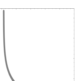
Figure 8: The evolution of the gauge coupling constant $g$ in the magnetic phase for N=2 (thick grey line) and N=3 (thick black line). The gauge coupling constant diverges logarithmically, $g\propto-\log(\lambda_{M}-\lambda_{M,c})$, at $\lambda_{M,c}=6.41$ (N=2) and $\lambda_{M,c}=5.82$ (N=3).

The gauge coupling constant $g$ increases continuously from $g=0$ at the electric-magnetic phase boundary ($\lambda_{M}=\lambda_{E,c}$) until it diverges logarithmically at $\lambda_{M,c}$. A continuous behavior of the magnetic coupling is not in contradiction with magnetic charge conservation since no isolated magnetic charges appear in the magnetic phase: magnetic monopoles are only present in condensed form, and there are no collective monopole excitations, see Eq. (88). The continuous rise of $g$, starting from zero at $\lambda_{M,c}$, implies a continuous behavior of the mass parameter $a$ in Eq. (3.3). Since $a$ is the measurable order parameter for monopole condensation this situation is reminiscent of a 2${}^{\tiny\mbox{nd}}$ order phase transition. We compute the critical exponent of this transition for N=2 in Sec. 3.5.

Lowering $\lambda_{M}$ towards $\lambda_{M,c}$ the core size of ANO vortices becomes large, the monopole condensates are more and more distorted by magnetic flux lines, and thus it becomes increasingly irrelevant in what SU(2) embedding a particular monopole lives. Formerly unstable monopoles acquire longevity and thus additional monopole condensates form at $\lambda_{M,c}$: $\bar{\varphi}_{i}\not=0\,,\ (i=\mbox{N}/2+1,\cdots,\mbox{N}-1)$ for $\lambda_{M}\sim\lambda_{c,M}$. As a consequence, all dual gauge-boson fluctuations $\delta a^{D}_{\mu,k}\,,\ (k=1,\cdots,\mbox{N}-1)$ are very massive close to $\lambda_{M,c}$ and decouple thermodynamically at $\lambda_{M,c}$. The equation of state at $\lambda_{M}=\lambda_{c,M}$ thus is

$$\rho(\lambda_{M,c})=-P(\lambda_{M,c})\,.$$ (99)

At $\lambda_{M,c}$, where all dual gauge-field fluctuations are very massive, the continuous dual gauge symmetry $U(1)_{D}^{\tiny\mbox{N-1}}$ is broken completely.

3.4 Polyakov loop in the electric and the magnetic phase

In this section we show that the Polyakov loop, which is an order parameter for the deconfining transition, indeed is finite in the electric and close to zero in the magnetic phase. In each phase the Polyakov loop of the full effective theory (now we also consider the fluctuations $\delta a_{\rho}$) formulated in Euclidean spacetime and unitary gauge is defined as

$${\bf P} = Z^{-1}\times\exp[-S_{cl}]\times\int{\cal D}\delta b_{\rho}\,\exp\left[-i\gamma\int_{0}^{T^{-1}}d\tau\,\delta b_{4}^{b.g.}\right]\times$$ (100)

$$\exp\left[-\int_{0}^{T^{-1}}d\tau d^{3}x\left\{\frac{1}{4}G^{2}[\delta b_{\rho}]+\sum_{k}m^{2}_{k}\,\delta b_{\mu,k}\delta b_{\mu,k}\right\}\right]\,.$$

where $\gamma=\{e,g\}$ and $\delta b_{\rho}=\{\delta a_{\rho},\delta a^{D}_{\rho}\}$ depending on whether we discuss the electric or the magnetic phase. The term $\exp[-S_{cl}]$ refers to the vanishing weight of the ground state in the partition function $Z$ in either phase. This weight, however, cancels in expectation values.

Figure 9: The data set used for the fit of the critical exponent $\nu$.

Since the fluctuations $\delta b_{\rho}$ are periodic in time they are decomposed as

$$\delta b_{\rho}(\tau,{\vec{x}})=\sum_{n=-\infty}^{n=\infty}\exp\left[2\pi in\frac{\tau}{T}\right]\bar{b}_{\rho,n}({\vec{x}})\,.$$ (101)

Modes with $n\not=0$ make the Polyakov-loop phase in Eq. (100) unity, are action-suppressed, and thus they are irrelevant. Zero modes ($n=0$) make a contribution to the Polyakov-loop phase if they are not action-suppressed. This is the case if both of the following conditions are met: (i) there is no mass term for these fluctuations and (ii) we have $\partial_{i}\bar{b}_{\rho,0}({\vec{x}})\sim 0$ where $\partial_{i}$ denotes a spatial derivative. In the electric phase TLM modes are massless and thus their space-indepent zero-mode fluctuations generate the bulk of the (finite) Polyakov loop. For N=2,3 there are no massless fluctuations in the magnetic phase and thus condition (i) is violated. As a consequence, none of the fluctuations $\delta b_{\rho}$ can contribute to the Polyakov loop in a substantial way in the magnetic phase and thus we have ${\bf P}\sim 0$. For N$>$3 the presence of unstable magnetic monopoles in the magnetic phase prevents some of the TLM modes to pick up a mass by the Abelian Higgs mechanism. Thus the Polyakov loop should be small but nonvanishing in the magnetic phase.

3.5 Critical exponent for the SU(2) electric-magnetic transition

In this section we compute the critical exponent $\nu$ for the electric-magnetic transition for N=2. The obvious order parameter for this transition is the ‘photon’ mass.

The data set in Fig. 9 is generated from an inversion of the numerical solution to the evolution equation Eq. (95). The following model is used to fit the data

$$a(\lambda_{M})=C\times|\lambda_{M}-\lambda_{M,em}|^{\nu}$$ (102)

where $C$ and $\nu$ are constants, $\lambda_{M,em}$ denotes the critical temperature $T_{e,c}$ in units of $\frac{\Lambda_{M}}{2\pi}$, and $a$ is the dimensionless ‘photon’ mass. Recall, that the value $\lambda_{E,c}=11.65$ is obtained from the position of the logarithmic pole of the coupling constant $e$ in the electric phase. By matching the pressure at the electric-magnetic phase boundary, see Sec.5, this translates into a value $\lambda_{M,em}=7.337$.

To perform the actual fit we have used Mathematica’s NonlinearFit function which is contained in the statistics package. In Fig. 10 the critical behavior of the ‘photon’ mass $a$ is shown.

Figure 10: The function $a(\lambda_{M})$ in the vicinity of the electric-magnetic phase transition. The region between the dashed vertical lines corresponds to the data set in Tab. 1 which generates the least sensitivity of $\nu$ on the length of the fitting interval $\Delta=|\lambda_{M,\tiny\mbox{min,fit}}-\lambda_{M,em}|$.

To determine the length of the fitting interval $\Delta=|\lambda_{M,\tiny\mbox{min,fit}}-\lambda_{M,em}|$ where $\nu$ is least sensitive to changes in $\lambda_{M,\tiny\mbox{min,fit}}$ we numerically determine the inflexion point $\Delta_{\tiny\mbox{inflex}}$ of the function $\nu=\nu(\Delta)$, see Fig. 11. We obtain

$$\Delta_{\tiny\mbox{inflex}}=0.29\pm 0.05\,.$$ (103)

We emphasize that this interval is well contained in the fitting interval used in [56] where the critical exponent was determined from the expectation of the dual string tension. Their fit interval $0\leq t\leq 1$ with $t\equiv\frac{T_{M,em}-T}{T_{M,em}}$ correponds to an interval length $\Delta=\lambda_{M,em}\sim 7.34$!

The interval of least senstivity $\Delta_{\tiny\mbox{inflex}}=0.29\pm 0.05$ translates into

$$\nu=0.61+0.02-0.01\,.$$ (104)

Alternatively, we can determine $\nu$ by a fit in very small intervals around $\lambda_{M,em}$. In this case we obtain the result expected from a naive mean-field analysis, $\nu\to 0.5$. However, the fitted prefactor $C$ varies considerably for very small intervals around $\lambda_{M,em}$. It is worth mentioning at this point that the ‘would-be’ critical exponent for N=3 has at least two inflexion points as a function of $\Delta$. This makes a unique determination of the physical value of $\nu$ impossible and clearly indicates that the phase transition is not second order anymore. A small latent heat is associated with the electric-magnetic transition for N=3, see Fig. 19, which makes it weakly first order. This is seen on the lattice [68].

The critical exponent for the 3D Ising model (same universality class as SU(2) Yang-Mills [57, 58]) is $\nu_{\tiny\mbox{Ising}}\sim 0.63$. As it seems, the effective theories for the electric and the magnetic phases have passed an important test!

4 The center phase

4.1 Isolated center vortices in the magnetic phase

Away from the points $\lambda_{E,c}$ and $\lambda_{M,c}$ there are isolated vortices in the magnetic phase which form closed loops due to the conservation of magnetic flux. Along the core region of a vortex, where the monopole condensate vanishes, $\bar{\varphi}_{k}\approx 0$, monopoles and antimonopoles form a closed chain and move into opposite directions [53]. Along a vortex loop the magnetic flux is $2\pi\,k/N\,,\ (k=1,\cdots,\mbox{N}-1)$ with respect to the dual gauge field $a^{D}_{\mu,k}$. This coins the name center vortex loop.

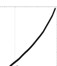
Figure 11: Dependence of the critical exponent $\nu$ on the length of the fitting interval $\Delta=|\lambda_{M,\tiny\mbox{min}}-\lambda_{M,c}|$. The inflexion point of the curve is at $\Delta_{\tiny\mbox{inflex}}=0.29\pm 0.05$ corresponding to $\nu=0.61+0.02-0.01$.

The typical action $S_{\tiny\mbox{ANO}}$ and energy $E_{\tiny\mbox{ANO}}$ of a center vortex loop can be estimated since an analytical solution to the Abelian Higgs model is known [54]:

$$S_{\tiny\mbox{ANO}}\sim\frac{1}{g^{2}}\,,\ \ \ \ \ \ \ E_{\tiny\mbox{ANO}}\propto\frac{1}{g}\,.$$ (105)

As a consequence of Eq. (105) center vortex loops do not carry action and are massless at $\lambda_{M,c}$ where $g$ diverges. They condense to form a new ground state of the system: a phase transition takes place. As we will show below this phase transition is nonthermal and of the Hagedorn type.

4.2 Center vortex condensates, macroscopically

Since center vortex loops are extended, one-dimensional objects the local scalar fields $\Phi_{k}(x)\,,\ (k=1,\cdots,\mbox{N}-1)$ describing their respective condensates have to be defined in a nonlocal way. We formally define the fields $\Phi_{k}(x)$ in terms of an average over the dual Abelian gauge fields $A^{D}_{\mu,k}$ of the magnetic phase (the part belonging to an ANO or center vortex is included in $A^{D}_{\mu,k}$!) as

$$\frac{\Phi_{k}(x)}{|\Phi_{k}(x)|}=\left\langle\exp\left[ig\oint dz_{\mu}A^{D}_{\mu,k}\right]\right\rangle_{A^{D}_{\mu,k}}\,.$$ (106)

In Eq. (106) the integration contour is spatial and circular, its center is at $x$, and circle’s diameter is infinite. In absence of a Yang-Mills scale $\Lambda_{C}$, which is a relevant situation when investigating the ground-state structure in the center phase due to the missing gauge-mode propagation, only dimensionless quantities like in Eq. (106) can be computed. As we shall see below, the presence of $\Lambda_{C}$ can only be observed in the excitation spectrum (selfintersections of center-vortices). We may always chose a parametrization of the integration contour $z(\xi)$ in Eq. (106) such that $0\leq\xi\leq 1$.

A (local) magnetic center rotation can be expressed as

$$\Omega(z)=\exp\left[\frac{2\pi i}{\mbox{N}}\sum_{k=1}^{\tiny\mbox{N-1}}\chi_{k}(z)\right]\,$$ (107)

where $\chi_{k}(z)$ is either $k$ or zero. The dual gauge field $A^{D}_{\mu,k}$ transforms under $\Omega(z)$ as

$$A^{D}_{\mu,k}\to A^{D}_{\mu,k}-g^{-1}\frac{2\pi}{\mbox{N}}\partial_{\mu}\chi_{k}(z)\,.$$ (108)

Figure 12: The phase of a local magnetic center transformation along a circular contour parametrized by $0\leq\xi\leq 1$ and its decomposition into boxes.

According to the definition (106) a magnetic center rotation $\Omega(z)$ may locally add a magnetic flux quantum [55] to the flux contained in $\Phi_{k}$. This is possible since we may have $\Omega(z(0))\not=\Omega(z(1))$. The action of the local magnetic center rotation $\Omega(z)$ on the complex field $\Phi_{k}(x)$ is as follows:

$$\Phi_{k}(x)\to\left\{\begin{array}[]{c}\exp[\pm\frac{2\pi ik}{\tiny\mbox{N}}]\,\Phi_{k}(x),\ \ \ (|\chi_{k}(z(1))-\chi_{k}(z(0))|=k)\,,\\ \,\,\,\,\,\Phi_{k}(x)\,,\ \ \ \ \ \ \ \ \ \ \ \ \ \ \ \mbox{otherwise}\end{array}\right.\,.$$ (109)

Obviously, the action of $\Omega(z)$ on $\Phi_{k}(x)$ may locally change the phase of the field $\Phi_{k}$, and thus the ground state is not invariant under local magnetic center transformations: $Z_{\mbox{N,mag}}$ as a discrete gauge symmetry is spontaneously broken in the center phase.

The local center transformation $\Omega$ singles out possible ‘boundaries of the circle’ at the positions $z(\xi_{n})$, ($\xi_{0}=0,\cdots$), where it jumps, see Fig. 12. The size and direction of an $\Omega$-induced magnetic flux quantum - an observable quantity - should not depend on the admissible re-parametrizations $\xi(\zeta)$, $(0\leq\zeta\leq 1)$ with $\xi(0)\in\{\xi_{n}\}$. For example, a translation

$$\xi(\zeta)=\zeta+\xi_{1}$$ (110)

would have shifted the ‘boundary of the circle’ at $z(\xi=0)$ to $z(\xi=\xi_{1})$. Thus it would have generated a different flux quantum. To avoid such an ambiguity we have to impose that a reparametrization of the circle is compensated for by an according local permutation of the fields $\Phi_{k}(x)$: if flux quanta $\frac{2\pi k}{\mbox{N}}$ and $\frac{2\pi l}{\mbox{N}}$, ($l\not=k$), were generated by $\Omega$ in the parameterizations $\xi$ and $\zeta$, respectively, then a permutation with $\Phi_{l}\to\Phi_{k}$ needs to be performed after the reparametrization $\zeta$ was implemented. This yields the same flux quantum as in parametrization $\xi$. Now, the discontinuous phase change in Eq. (109) is provided by the dynamics in an effective theory and is not externally imposed. As a consequence, the demand for invariance of a generated flux quantum under admissible contour-reparametrizations translates into an invariance of the effective Lagrangian under local permutations of the set $\{\Phi_{1}(x),\cdots,\Phi_{\tiny\mbox{N-1}}(x)\}$. The following Lagrangian satisfies this requirement:

$${\cal L}_{C}=\frac{1}{2}\sum_{k=1}^{\tiny\mbox{N-1}}\left[\partial_{\mu}\Phi_{k}\partial_{\mu}\Phi_{k}+V_{C}(\Phi_{k})\right]\,.$$ (111)

It is clear from Eq. (111) that the transformation in Eq. (109) is only a symmetry of the potential term due to the noninvariance of the kinetic terms under the jumps in the fields $\Phi_{k}$. However, because of the conservation of magnetic flux (only closed loops of center vortex flux can be generated) one quantum of center flux created by a jump at one point in spacetime is compensated by an opposite quantum of center flux created by the opposite jump at another point. The spacetime integral over ${\cal L}_{C}$, the action, is therefore invariant under local center rotations which induce magnetic flux in a closed flux line. Based on the continuum Lagrangian in Eq. (111) it would be interesting to perform a lattice simulation of the transition to the center phase taking any member of the set $\{|\Phi_{k}|\}$ as an order parameter.

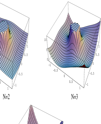
Figure 13: The potential $V_{C}=\overline{v_{C}(\Phi)}v_{C}(\Phi)$ corresponding to the definition in Eq. (112) for N=2,3,4 and $\Lambda_{C}=\Lambda^{\prime}_{C}$. $|\Phi|$ is given in units of $\Lambda_{C}$ and $V_{C}$ in units of $\Lambda_{C}^{4}$. Notice the minima $V_{C}=0$ at the N${}^{\tiny\mbox{th}}$ unit roots.

The function $V_{C}(\Phi)$ in Eq. (111) can be written as $V_{C}(\Phi)=\overline{v_{C}(\Phi)}v_{C}(\Phi)$. Let us now discuss the properties of the function $v_{C}$. If a matching to the magnetic phase would take place in thermodynamical equilibrium and a classical treatment of the ground-state dynamics could be justified at this point then the Euclidean time dependence of the (periodic) fields $\Phi_{k}$ would have to be BPS saturated. Only in this case do the fields $\Phi_{k}$ describe the condensates of zero-energy center-vortex loops .

At first sight a candidate for $v_{C}$ would be $v_{C,\tiny\mbox{trial}}(\Phi_{k})=i\Lambda_{C}^{3}/\Phi_{k}$. The potential $V_{C}$ would then not only be $Z_{\tiny\mbox{N,mag}}$ but also $U(1)^{\tiny\mbox{N-1}}$ symmetric. The latter (global) symmetry, however, does not exist in SU(N) Yang-Mills theory and thus $v_{C,\tiny\mbox{trial}}$ is excluded.

A function $v_{C}(\Phi_{k})$, which is covariant only under $Z_{\tiny\mbox{N}}$ transformations and, at the same time, allows for periodic and BPS saturated solutions along the Euclidean time coordinate $\tau$ [49], see Fig. 14,

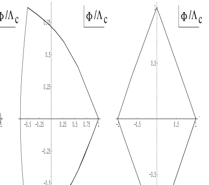
Figure 14: Numerical solutions to the BPS equation $\partial_{\tau}\Phi=\overline{v_{C}(\Phi)}$ for N=2,3,4.

, is uniquely given as

$$v_{C}(\Phi_{k})=i\left(\frac{\Lambda_{C}^{3}}{\Phi_{k}}-\frac{\Phi_{k}^{\tiny\mbox{N-1}}}{(\Lambda^{\prime}_{C})^{\tiny\mbox{N-3}}}\right)\,$$ (112)

where $\Lambda_{C}$ and $\Lambda^{\prime}_{C}$ denote mass scales that are a priori independent. The N degenerate minima of the potential $V_{C}(\Phi_{k})$ are at

$$|\Phi^{\tiny\mbox{min}}_{k}|=\left[\Lambda_{C}^{3}(\Lambda^{\prime}_{C})^{\tiny\mbox{N-3}}\right]^{1/\tiny\mbox{N}}\,.$$ (113)

At these minima the potential $V_{C}$ vanishes. Periodic solutions to the BPS equations

$$\partial_{\tau}\Phi_{k}=\bar{v_{C}(\Phi_{k})}$$ (114)

are parameterized by a winding number $\in\bf{Z}$ in analogy to the situation in the magnetic phase. The fields $\Phi_{l}\,,\ \ (l=1,\cdots,\mbox{N}/2)$, which are associated with vortices formed from the stable dipoles of the electric phase, are winding accordingly. For the fields $\Phi_{i}\,,\ \ (i=\mbox{N}/2+1,\cdots,\mbox{N}-1)$, being associated with vortices formed from independent monopoles, which are unstable in the electric phase, no winding numbers can be derived. This uncertainty in assigning winding numbers for the fields $\Phi_{i}$ is reflected in the appearance of an additional mass scale $\Lambda^{\prime}_{C}$ in Eq. (112). In the cases N=2,3, however, only stable, independent monopoles exist, and thus we can set $\Lambda_{C}=\Lambda^{\prime}_{C}$.

In Fig. 13 the graphs of the potential $V_{C}$ for N=2,3,4 and for $\Lambda_{C}=\Lambda^{\prime}_{C}$ are shown. Notice the ridges and the valleys of negative and positive tangential curvature, respectively. Due to the BPS saturation a solution $\Phi_{k}$ to Eq. (114) is guaranteed to carry no energy. This statement is, however, only then useful for the description of the ground state if the classical approximation can be justified. At finite N the modulus of BPS saturated solutions is no longer $\tau$ independent, see Fig. 14. On the one hand, this situation is in contradiction to thermal equilibrium. On the other hand, we can not trust the classical approximation since tangential fluctuations $\theta_{k}$, defined as

$$\Phi_{k}=|\Phi_{k}|\exp[i\frac{\theta_{k}}{\Lambda_{C}}]\,,$$ (115)

can be tachyonic and therefore destabilize the classical solution to Eq. (114), see Fig. 15. In the electric and the magnetic phase tangential fluctuations of the caloron and the monopole condensates are would-be Goldstone modes giving rise to longitudinal polarizations of gauge boson fluctuations. Due to the absence of a continuous gauge symmetry in the center phase no gauge-field fluctuations exist which could ‘eat’ the tangential fluctuations. How to integrate out tachyonic tangential modes analytically is conceptually unclear. The only definite statement we can make at present is that they rapidly drive the expectation of the fields $\Phi_{k}$ towards the minima of $V_{C}$: $\Phi_{k}$ relaxes to one of the minima of $V_{C}$ along an outward directed spiral in the complex plane. During this process magnetic flux quanta are locally generated by discontinuous phase changes of $\Phi_{k}$ due the tunneling through the regions where the tangential fluctuations are tachyonic.

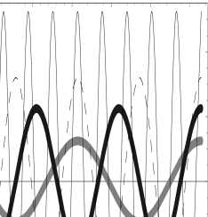
Figure 15: The ratio $\left.\partial^{2}_{\theta_{k}}V_{C}(\Phi_{k})/|\Phi_{k}|^{2}\right|_{|\Phi_{k}(0)|=0.8\Lambda_{C}}$ ($V_{C}$ defined in Eq. (112) and $\Lambda_{C}=\Lambda_{C}^{\prime}$) as a function of $\frac{\theta_{k}}{\Lambda_{C}}$ for N=2 (thick grey line), N=3 (thick black line), N=4 (dashed line), and N=10 (thin solid line).

Once the field $\Phi_{k}$ has settled into one of the minima of $V_{C}$ the situation is classical again. At the minima we have

$$\left.\frac{\partial^{2}_{\theta_{k}}V_{C}(\Phi_{k})}{|\Phi_{k}|^{2}}\right|_{\Phi^{\tiny\mbox{min}}_{k}}=\left.\frac{\partial^{2}_{|\Phi_{k}|}V_{C}(\Phi_{k})}{|\Phi_{k}|^{2}}\right|_{\Phi^{\tiny\mbox{min}}_{k}}=2\mbox{N}^{2}>1\,.$$ (116)

The approximation $\Lambda_{C}=\Lambda_{C}^{\prime}$ used in Eq. (116) is exact for N=2,3. Since radial and tangential quantum fluctuations are heavier than the compositeness scale $\Phi^{\tiny\mbox{min}}_{k}$ they are absent in the effective theory. As a consequence, the vanishing value of $V_{C}$ at the minima receives no radiative corrections.

In the limit $\mbox{N}\to\infty$ only the pole term of the potential $V_{C}$ survives for $|\Phi_{k}|<|\Phi^{\tiny\mbox{min}}_{k}|$ and thus we recover the situation of a global $U(1)^{\tiny\mbox{N}-1}$ symmetry. The $\tau$ dependence of the solutions to the BPS equation (114) is then a pure phase and no tachyonic but only massless tangential fluctuations exist. These fluctuations lead to an instantaneous reheating at the phase boundary. The order parameter $|\Phi_{k}|$ jumps from zero to a finite value across the phase boundary. While the energy density of the ground-state jumps to zero at the phase boundary (BPS saturation), the ground-state pressure jumps to zero only after $|\Phi_{k}|=|\Phi^{\tiny\mbox{min}}_{k}|$ is reached.

At finite N a flux quantum and a radial displacement $\Delta|\Phi_{k}|$ are generated in each tunneling process. This reduces the ground-state energy density locally and brings the field $\Phi_{k}$ closer to one of the minima of $V_{C}$. The closer $\Phi_{k}$ to a minimum the less likely a tunneling process since the associated energy gain is quickly reduced ($|\partial_{|\Phi_{k}|}V_{C}|$ decreases!). If the number of tunneling processes taking place until relaxation would be roughly independent of N then for small N many unit-root directions will be reached in a relaxation process and thus it is likely that the average value of $\Phi_{k}$ close to the phase boundary is close to zero. For large N only a small angular sector would be reached by tunneling and thus close to the phase boundary the average value of $\Phi_{k}$ is not close to zero: a strong discontinuity of $\Phi_{k}$ across the transition should be observed.

Closed center-vortex flux lines can self-intersect and in this way form isolated $Z_{\tiny\mbox{N}}$ monopoles which reverse the flux, see Fig. 16 for the N=2 case.

Figure 16: The creation of an isolated $Z_{2}$ monopole by self-intersection of a $Z_{2}$ center vortex.

Let us discuss the case N=2 more explicitly. During the phase transition the process leading to self intersection can be performed $L$ times on a nonintersecting vortex loop. This generates $L$ isolated $Z_{2}$ monopoles, each of mass $\sim\Lambda_{C}$, such that the mass $M_{L}$ of the $L$-monopole state is $M_{L}\sim L\Lambda_{C}$. Since the number of possible $L$-monopole states roughly grows as $L!$ (see [69] for a more precise estimate) we conclude that the density of states $\rho(E)$ for the particle excitations in the center phase of an SU(2) theory is over-exponentially growing in energy $E$:

$$\rho(E)>\Lambda_{C}\exp\left[\frac{E}{\Lambda_{C}}\right]\,.$$ (117)

For N$>$2 the situation is similar. So we conclude that there exists a highest temperature $T_{\tiny\mbox{H}}\sim\Lambda_{C}$ in the center phase of an SU(N) Yang-Mills theory: a situation which was anticipated for any strongly interacting four dimensional field theory a long time ago [10], see also [60] for a discussion of the Hagedorn transition in an SU(N) matrix model. Moreover, we conclude that the center-magnetic phase transition can by no means be thermal (the spatial homogeneity of the system is violated during the transition) and thus that the thermodynamical pressure may jump across the transition. A single and a one-time self-intersecting center-vortex loop for N=2 are fermions [59]. This result is crucial for our understanding of the nature of leptons in the present Standard Model of Particle Physics. The time scale for the relaxation to one of the minima of $V_{C}$ is roughly given by $|(\Phi^{\tiny\mbox{vac}}_{k})|^{-1}$. A quantitative investigation of this reheating process would need methods of nonequilibrium field theory, see for example [61]. In a thermal approach it would be interesting to check in a lattice simulation of the effective theory in the center phase Eq. (111) whether a density of states as in Eq. (117) is indeed seen.

The fact that the pressure and the energy density of the ground state are precisely vanishing at the minima $\Phi^{\tiny\mbox{vac}}_{k}$ and that there are no radiative corrections to this situation clearly is of cosmological relevance.

5 Scale matching

The scales $\Lambda_{E}$ and $\Lambda_{M}$, which determine the magnitudes of the adjoint Higgs field $\phi$ and the monopole condensates $\varphi_{l}$ at a given temperature in the electric and the magnetic phase, can be related by imposing the condition that the thermodynamical pressure $P$ be continuous across the thermal electric-magnetic phase transition. Disregarding the mismatch in the number of polarizations for some TLM modes in the electric phase and some dual gauge bosons in the magnetic phase, we derive

$$\Lambda_{E}=(1/4)^{1/3}\Lambda_{M}\,\ \ \ \ (\mbox{N\ \ even})\,.$$ (118)

For N=3 we have $\Lambda_{E}=(1/2)^{1/3}\Lambda_{M}$. The match between the magnetic and the center phase is less determined for the following reasons: (i) For N$>$3 the winding numbers of the fields $\Phi_{i}\,\ \ (i=\mbox{N}/2+1,\cdots,\mbox{N}-1)$ close to the center-magnetic phase boundary are dynamically generated during the phase transition and so cannot be derived from the boundary conditions for the electric phase. For N=2 and N=3 the winding numbers of $\Phi_{1}$ and $(\Phi_{1},\Phi_{2})$ are unity, and we can set $\Lambda_{C}=\Lambda^{\prime}_{C}$ in Eq. (112). (ii) An analytical description based on the potential $V_{C}$ of the center-magnetic phase transition at finite N breaks down at the phase boundary, see Sec. (4).

In the electric and in the magnetic phase (recall that the latter confines fundamental test charges) we encounter the thermodynamical analogue to dimensional transmutation in perturbation theory: Assuming MGSB, a single, fixed mass scale determines the thermodynamics of the SU(N) Yang-Mills theory in these phases. At a given temperature this mass scale can be experimentally inferred from the mass spectrum of the gauge boson fluctuations.

6 Pressure, energy density, and entropy density

6.1 Numerical results

In this section we present our numerical results for one-loop temperature evolutions of thermodynamical potentials through the electric and magnetic phase. For the actual computations we consider N=2,3 only.

In the electric phase the pressure $P$ divided by $T^{4}$ is given as

$$\frac{P}{T^{4}}=-\frac{(2\pi)^{4}}{\lambda_{E}^{4}}\left[\frac{2\lambda_{E}^{4}}{(2\pi)^{6}}\left\{2\,(\mbox{N}-1)\bar{P}(0)+3\sum_{k=1}^{\tiny\mbox{N(N-1)}}\bar{P}(a_{k})\right\}+\frac{\lambda_{E}}{2}\left(\frac{\mbox{N}}{2}+1\right)\mbox{N}\right]\,,\ \ (\mbox{N\ \ even})\,,$$ (119)

where the function $\bar{P}(a)$ and the dimensionless mass parameters $a_{k}$ are defined in Eqs. (43) and (40), respectively, and MGSB is assumed. In the magnetic phase we have

$$\frac{P}{T^{4}}=-\frac{(2\pi)^{4}}{\lambda_{M}^{4}}\left[\frac{2\lambda_{M}^{4}}{(2\pi)^{6}}\left\{2\,(\frac{\mbox{N}}{2}-1)\bar{P}(0)+3\sum_{l=1}^{\tiny\mbox{N}/2}\bar{P}(a_{l})\right\}+\frac{\lambda_{M}}{16}\mbox{N}(\mbox{N}+2)\right]\,,\ \ (\mbox{N\ \ even})\,.$$ (120)

The dimensionless mass parameters $a_{l}$ are defined in Eqs. (93) and Eq. (3.3)).

For N=3 we have in the electric and the magnetic phase, respectively:

$$\frac{P}{T^{4}} = -\frac{(2\pi)^{4}}{\lambda_{E}^{4}}\left[\frac{2\lambda_{E}^{4}}{(2\pi)^{6}}\left\{4\bar{P}(0)+3\left(4\,\bar{P}(a)+2\,\bar{P}(2a)\right)\right\}+2\lambda_{E}\right]\,,\ \ (\mbox{N=3})\,,$$

$$\frac{P}{T^{4}} = -\frac{(2\pi)^{4}}{\lambda_{M}^{4}}\left[\frac{12\lambda_{M}^{4}}{(2\pi)^{6}}\bar{P}(a)+\lambda_{M}\right]\,,\ \ (\mbox{N=3})\,.$$ (121)

The mass parameters $a_{k}$ and $a_{l}$ evolve with temperature according to the (inverted) solutions to Eqs. (50), (51), (95), and (96).

Our results for $\frac{P}{T^{4}}$ as a function of temperature in the electric and magnetic phase are shown in Fig. 17.

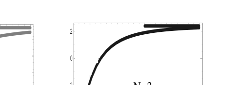
Figure 17: $\frac{P}{T^{4}}$ as a function of temperature for N=2,3. The horizontal lines denote the respective asymptotic values. For N=2 we have $\lambda_{E,c}=11.65$ and for N=3 $\lambda_{E,c}=8.08$.

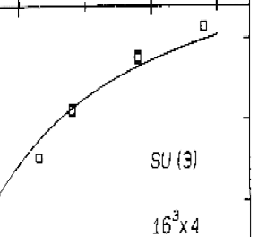
Figure 18: $\frac{P}{T^{4}}$ as a function of temperature for N=3 as obtained on a $16^{3}\times 4$ lattice using the differential method with a universal two-loop perturbative $\beta$ function [65, 66] and using the integral method (solid line) [67]. The figure is taken from [67].

Notice that the pressure is negative in the electric phase close to $\lambda_{E,c}$ and even more so in the magnetic phase where the ground-state strongly dominates the thermodynamics.

In the electric phase the energy density $\rho$ divided by $T^{4}$ is given as

$$\frac{\rho}{T^{4}}=\frac{(2\pi)^{4}}{\lambda_{E}^{4}}\left[\frac{2\lambda_{E}^{4}}{(2\pi)^{6}}\left\{2\,(\mbox{N}-1)\bar{\rho}(0)+3\sum_{k=1}^{\tiny\mbox{N(N-1)}}\bar{\rho}(a_{k})\right\}+\frac{\lambda_{E}}{2}\left(\frac{\mbox{N}}{2}+1\right)\mbox{N}\right]\,,\ \ (\mbox{N\ \ even})\,,$$ (122)

where the function $\bar{\rho}(a)$ is defined as

$$\bar{\rho}(a)\equiv\int_{0}^{\infty}dx\,x^{2}\frac{\sqrt{x^{2}+a^{2}}}{\exp(\sqrt{x^{2}+a^{2}})-1}\,.$$ (123)

In the magnetic phase we have

$$\frac{\rho}{T^{4}}=\frac{(2\pi)^{4}}{\lambda_{M}^{4}}\left[\frac{2\lambda_{M}^{4}}{(2\pi)^{6}}\left\{2\,(\frac{\mbox{N}}{2}-1)\bar{\rho}(0)+3\sum_{l=1}^{\frac{\tiny\mbox{N}}{2}}\bar{\rho}(a_{l})\right\}+\frac{\lambda_{M}}{16}\mbox{N}(\mbox{N}+2)\right]\,,\ \ (\mbox{N\ \ even})\,.$$ (124)

For N=3 we have in the electric and the magnetic phase, respectively:

$$\frac{\rho}{T^{4}} = \frac{(2\pi)^{4}}{\lambda_{E}^{4}}\left[\frac{2\lambda_{E}^{4}}{(2\pi)^{6}}\left\{4\bar{\rho}(0)+3\left(4\,\bar{\rho}(a)+2\,\bar{\rho}(2a)\right)\right\}+2\lambda_{E}\right]\,,\ \ (\mbox{N=3})\,,$$

$$\frac{\rho}{T^{4}} = \frac{(2\pi)^{4}}{\lambda_{M}^{4}}\left[\frac{12\lambda_{M}^{4}}{(2\pi)^{6}}\bar{\rho}(a)+\lambda_{M}\right]\,,\ \ (\mbox{N=3})\,.$$ (125)

Our results for $\frac{\rho}{T^{4}}$ as a function of temperature in the electric and magnetic phase are shown in Fig. 19. Slight discontinuities at $\lambda_{E,c}$ are seen. This is explained by the mismatch in the number of polarizations of fluctuating gauge bosons across the electric-magnetic transition - an approximation to scale-matching - and the fact that continuity in $P$ does not imply continuity in $\rho$. Again, the energy density is dominated by the ground-state contribution in the electric phase close to the electric magnetic transition and even more so in the magnetic phase.

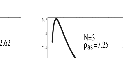
Figure 19: $\frac{\rho}{T^{4}}$ as a function of temperature for N=2,3. The horizontal lines denote the respective asymptotic values.

The entropy density $S$ is defined as the derivative of the pressure with respect to temperature:

$$S\equiv\frac{dP}{dT}\,.$$ (126)

Using the thermodynamical relation $\rho=T\frac{dP}{dT}-P$, we may write

$$\frac{S}{T^{3}}=\frac{1}{T^{4}}\left(\rho+P\right)\,.$$ (127)

Our results for $S/T^{3}$ are shown in Fig. 20. The reasons for the slight discontinuities at $\lambda_{E,c}$ are the same as in the case $\frac{\rho}{T^{4}}$. The entropy density $S$ is a measure for the ‘mobility’ of gauge boson excitations. That $S$ is zero at the critical temperature $\lambda_{M,c}$ for the center transition is explained by the fact that all dual gauge bosons acquire an infinite mass there and thus no fluctuating degrees of freedom are left in the thermodynamical balance.

6.2 Comparison with the lattice

An early lattice measurements of the energy density $\rho$ and the interaction measure $\Delta\equiv\rho-3P$ in a pure SU(2) gauge theory were reported on in [62]. In that work the critical temperature $T_{c}$ for the deconfinement transition was determined from the critical behavior of the Polyakov-loop expectation and the peak position of the specific heat using a Wilson action. The function $\Delta(T)$ was extracted by multiplying the lattice $\beta$ function with the difference of plaquette expectations at finite and zero temperature. This assures that $\Delta$ vanishes as $T\to 0$. What is subtracted at finite $T$ is, however, not the value $\Delta(T=0)$ since the associated plaquette expectation is multiplied with the value of the $\beta$ function at finite $T$. Apart from this approximation, the use of a perturbative $\beta$ function was assumed for all temperatures.

Figure 20: $\frac{S}{T^{3}}$ as a function of temperature for N=2,3. The horizontal lines denote the respective asymptotic values.

The lattice results for $\rho$ differ drastically from our results for temperatures close the deconfinement, that is, the electric-magnetic transition. We obtain

$$\left.\frac{\rho}{\rho_{SB}}\right|_{T\sim T_{E,c}}\sim 1.49$$ (128)

where $\rho_{B}\equiv\frac{\pi^{2}}{5}T^{4}$ denotes the Stefan-Boltzmann limit (ideal gas of massless gluons with two polarizations). On the lattice, this ratio is measured to be smaller than unity. At $T\sim 5T_{E,c}$ we obtain

$$\left.\frac{\rho}{\rho_{SB}}\right|_{T\sim 5\,T_{E,c}}\sim 1.34\,$$ (129)

while the lattice measures a ratio of about 0.85. Our asymptotic value is

$$\left.\frac{\rho}{\rho_{SB}}\right|_{T\sim 6.4\,T_{E,c}}\sim 1.33\,.$$ (130)

Notice the latent heat released at the electric magnetic transition for N=3 (Fig. 19).

Our result for the pressure $P$ indicates negative values for $T$ close to $T_{E,c}$ (see Fig.  17) - much in contrast to the positive values obtained in [62]. At $T\sim 5T_{E,c}$ we obtain

$$\left.\frac{P}{P_{SB}}\right|_{T\sim 5\,T_{E,c}}\sim 1.30\,$$ (131)

while the lattice measures ($P$ is extracted from the measured values of $\Delta$ and $\rho$) a ratio of about 0.88. Our asymptotic value for $P$ is

$$\left.\frac{P}{P_{SB}}\right|_{T\sim 6.4\,T_{E,c}}\sim 1.32\,.$$ (132)

The asymptotic values of Eqs. (130) and (132) are very close to the ratio $R$ of the number of polarizations for massive TLH modes and massless TLM modes and the number of polarizations for massless gluon modes with two polarizations:

$$R=\frac{2\times 3+1\times 2}{3\times 2}=\frac{4}{3}\sim 1.33\,.$$ (133)

Indeed, at $\lambda_{E}\sim 75$ the mass parameter $a$, defined in Eq. (42), is $a\sim 2\pi\frac{5.5}{650}\sim 0.053$ and therefore the Boltzmann suppression of TLH modes is small. At extremely high temperatures a TLH mode ‘remembers’ its massiveness at low temperatures in terms of an extra polarization coming from a tiny mass which, however, still solves the infrared problem of naive perturbation theory.

For a comparison with N=3 lattice data we use the results obtained with a Wilson action in [63] on the lattice of the largest time extension, $N_{\beta}=8$. In the vicinity of the transition point $T_{E,c}$ the situation for both $\rho$ and $P$ is similar as for N=2: drastic differences between the lattice measurements and our results occur. Again, $P$ comes out negative in our calculation, contradicting the positive values obtained in [63]. It should be remarked at this point that a lattice simulation of $P$, which did not rely on the integral method (see below) as it was used in [63], has seen negative pressure for $T$ not far above $T_{c,e}$ [66]. Moreover, the most negative value of $P/T^{4}\sim-0.5$ obtained in [66] very close to the phase transition coincides with our result at the electric-magnetic transition, see Figs. 17 and 18.

At $T=5\,T_{E,c}$ we have

$$\left.\frac{\rho}{\rho_{SB}}\right|_{T\sim 5\,T_{E,c}}\sim 1.38$$ (134)

while the lattice measures a ratio of about 0.93. Our asymptotic value for $\rho$ is

$$\left.\frac{\rho}{\rho_{SB}}\right|_{T\sim 8.86\,T_{E,c}}\sim 1.37\,.$$ (135)

For the pressure $P$ we obtain at $T=5\,T_{E,c}$:

$$\left.\frac{P}{P_{SB}}\right|_{T\sim 5\,T_{E,c}}\sim 1.34\,$$ (136)

while the lattice measures a ratio of about 0.97. Our asymptotic value for $P$ is

$$\left.\frac{P}{P_{SB}}\right|_{T\sim 8.86\,T_{E,c}}\sim 1.36\,.$$ (137)

Both asymptotic values in Eqs. (135) and (137) are very close to the ratio of polarizations $R=\frac{11}{8}=1.375$.

According to Fig. (20) the entropy density $\frac{S}{T^{3}}$ vanishes at $T_{M,c}$. In our approach this reflects the fact that at $T_{M,c}$ all gauge-field are thermodynamically decoupled because of their infinite mass. As a consequence, thermodynamics is entirely determined by the ground state. This is not observed in the lattice simulations [64] for both N=2,3 where a continuous behavior of $\frac{S}{T^{3}}$ across the deconfinement transition at $T_{E,c}$ was obtained.

In [65] a discontinuous behavior of $\frac{S}{T^{3}}$ was observed for N=3 using a Wilson action and a perturbative beta function. There is an excellent agreement of their result with our result for temperatures ranging $T_{E,c}$ down to $T_{M,c}$, compare Figs. 20 and 21.

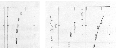
Figure 21: $\frac{S}{T^{3}}$ as a function of $\beta$ obtained in SU(3) lattice gauge theory using the differential method and a perturbative beta function. The simulations were performed on (a) $16^{3}\times 4$, (b) $24^{3}\times 4$, (c) $16^{3}\times 6$ (open circles) and $20^{3}\times 6$ (closed circles), and (d) $24^{3}\times 6$ lattices. Using the $24^{3}\times 6$ lattice, the critical value of $\beta$ is between 5.8875 and 5.90.

The almost discontinuous behavior in Fig. (20) is due to the large rise of the magnetic gauge coupling with decreasing temperature. According to Fig. (8) the ‘duration’ $\delta T\equiv\frac{T_{E,c}-T_{M,c}}{T_{E,c}}$ of the magnetic phase is only $\delta T\sim 0.1$. In a lattice simulation the resolution of such a small temperature interval depends very much on the choice of the beta function. In [65] a universal perturbative beta function was used which may have lead to interprete the behavior of $\frac{S}{T^{3}}$ as discontinuous in dependence on temperature. Since $\frac{S}{T^{3}}$ is a quantity which is much less sensitive to the infrared physics than, say, $\frac{P}{T^{4}}$ (the direct contribution of the ground state is canceled out in $\frac{S}{T^{3}}$) the use of (the universal part of) a perturbative beta function in the lattice simulations [65] may be justified. We stress at this point that lattice simulations based on lattice sizes of 1-3 times the inverse Yang-Mills scale are not capable of being sensitive to the infrared effects of the theory which have correlation lengths of the order of the gauge couplings $e$ and $g$ times the inverse Yang-Mills scale at decoupling (Standard Model physics in the electroweak sector suggest that $e_{\tiny\mbox{decoup}}\sim g_{\tiny\mbox{decoup}}\sim 10^{6}\,$!).

The alert reader would object that the thermodynamical relation

$$dP=S\,dT\,,$$ (138)

which implies that in a homogeneous thermal system the pressure has to be a monotonic function of temperature, is violated at the center transition ($T_{c,M}$), see Fig. 17, where with decreasing temperature the pressure quickly rises from a negative to a value close to zero . What is the resolution of this puzzle? There are two anwers. First, on a microscopic level, the homogeneity of the system at the point where center vortices start to condense is badly violated by the generation of (intersecting) center-vortex loops through discontinuous and local phase changes of the fields $\Phi_{k}(x)$ in Eq. (106). The derivation of Eq. (138) from the partition function, however, relies on homogeneity. Second, assuming homgeneity, one can easily convinces oneself that the spectral density $\rho(E)$ in the center phase is exponentially increasing with energy $E$:

$$\rho(E)\propto\exp[\frac{E}{T_{\tiny\mbox{H}}}]\,.$$ (139)

Thus the partition function diverges at $T=T_{\tiny\mbox{H}}\sim T_{c,M}$, the homogeneous system would need an infinite amount of energy per volume to increase the temperature beyond $T_{\tiny\mbox{H}}$. We conclude that homogeneity is violated at $T=T_{\tiny\mbox{H}}$. We conclude that the SU(N) YM dynamics indeed predicts a violation of the thermodynamical relation in Eq. (138) at $T=T_{\tiny\mbox{H}}\sim T_{c,M}$ .

What are the possible reasons for the qualitative difference between the results obtained in [63, 64] and [65, 66]? To avoid the use of derivatives of the bare coupling, which are multiplying the sum of spatial and time plaquette averages in the differential method for the computation of the pressure, the integral method was introduced in [67]. Using a perturbative beta function in the differential method, negative values for the pressure for $T$ close to $T_{c}$ and a rapid approach of the $\rho$ and $P$ to their respective ideal gas limits were obtained in [66]. The rapid approach to the ideal gas limit in $\rho$ is also obtained in the present approach, compare Eqs. (129), (130) and Eqs. (134),(135). At the time when the results in [65, 66] appeared a negative pressure was regarded as unphysical and attributed to the use of a perturbative beta function. The integral method proposed in [67] solely generates positive pressure. This method assumes the validity of the thermodynamical limit in the lattice simulation. Namely, for large spatial volume the thermodynamical relation

$$P=T\frac{\partial\ln Z}{\partial V}$$ (140)

valid for a finite volume $V$ is approximated by

$$P=T\frac{\ln Z}{V}\,$$ (141)

so that the pressure equals minus the free energy density. In Eqs. (140) and (141) $Z$ denotes the partition function. Based on Eq. (141) the derivative of the pressure with respect to the bare coupling $\beta=\frac{2\mbox{N}}{\bar{g}^{2}}$ can be expressed as an expectation over the sum of spatial and time plaquettes without the beta-function prefactor. Thus the pressure can be obtained by an integral over $\beta$ up to an unknown integration constant. The latter is chosen in such a way that the pressure vanishes at a temperature well below $T_{c}$. Instead of only integrating over minus the sum of spatial and time plaquette expectations twice the plaquette expectation at $T=0$ was added to the integrand in [63, 64] to assure that the pressure vanishes at $T=0$. We would like to stress that this prescription does not follow from relation (141). Thus it seems to be natural that integral and differential methods generate qualitatively different results. The results for $P(T)$ obtained by the integral method show a rather large dependence on the cutoff and the time extent $N_{\tau}$ of the lattice [63]. We believe that this reflects the considerable deviation from the assumed thermodynamical limit for so-far available lattice sizes. The problem was addressed in [64] where a correction factor $r$ was introduced to relate $P$ obtained with the integral method to $P$ obtained with the differential method. For a given $N_{\tau}$ the factor $r$ was determined from the pressure ratio at $\bar{g}=0$. Subsequently, this value of $r$ was used at finite coupling $\bar{g}$ to extract the spatial anisotropy coefficient $c_{\sigma}$ (essentially the beta function) by demanding the equality of the pressure obtained with the integral and the differential method. In doing so, twice the plaquette expectation at $T=0$ was, again, added to minus the sum of spatial and time plaquette expectations in the expression for the pressure using the differential method. It may be questioned whether a simple multiplicative correction $r$ does correctly account for finite-size and cutoff effects and, if yes, whether it is justified to determine $r$ in the limit of noninteracting gluons.

To summarize, we observe a qualitative disagreement between the lattice results [62, 63] for $\rho$ and $P$, using the integral method, and the results of the present approach for temperatures close to $T_{E,c}$. At $T\sim 5\,T_{E,c}$ there is better agreement. Although for N=3 our negative values for $P$ in the vicinity of $T_{E,c}$ disagree with those obtained with the differential method (we obtain a modulus at $T_{E,c}$ which coincides with that of the minimal value obtained by using a perturbative beta-function differential method [66]). On the other hand, the entropy density obtained in [65] with the differential method agrees well with our results. This is expected since the entropy is an infrared insensitive quantity.

7 Conclusions and Outlook

We have developed a nonperturbative approach to SU(N) Yang-Mills thermodynamics which is based on the (self-consistent) assumption that the theory ‘condenses’ SU(2) embedded, BPS saturated topological fluctuations of trivial holonomy at an asymptotically high temperature. In [34] we have shown for the SU(2) case the redundancy of this assumption. The concept for the construction of an effective theory based on the above assumption is similar to that applied to the construction of the macroscopic field theory for superconductivity [21, 22]. We stress that the effects on nontrivial topology die off in a power-like fashion in the effective theory (as a function of temperature). Thus the perturbatively derived suppression of topologically nontrivial field configurations does take place in our effective theory as well.

We have constructed a (uniquely determined) potential for the thermodynamics of an energy- and pressure-free adjoint Higgs background $\phi$ which macroscopically describes the collective effects due to noninteracting, trivial-holonomy calorons in the only deconfining phase of the theory which we call electric phase for obvious reasons. As a consequence, the ground state of the system is described by a BPS saturated solution to the field equation of the scalar sector and an associated pure-gauge configuration solving the macroscopic equation of motion for trivial-topology gauge-field fluctuations. The latter has macroscopic, nontrivial holonomy and thus describes the presence of isolated magnetic monopoles being generated from decaying nontrivial-holonomy calorons as a result of microscopic interactions between trivial-holonomy calorons. These interactions are mediated by the trivial-topology sector of the theory. The modulus of $\phi$ falls off as $\propto T^{-1/2}$ and the ground-state pressure is only linear in $T$ so that nonperturbative effects (apart from extra polarizations for excitations) are irrelevant at asymptotically high temperatures.

Some of the topologically trivial gauge-field fluctuations are massive on tree-level due to the adjoint Higgs mechanism, and the underlying SU(N) gauge symmetry is spontaneously broken accordingly. An evolution equation, describing the temperature dependence of the effective gauge coupling constant $e$, was obtained from the requirement of thermodynamical self-consistency of the effective theory. The two fixed points of this evolution were identified. These fixed points predict the existence of a highest and a lowest attainable temperature in the electric phase. Based on the evolution $e(T)$ a physical argument was given why caloron ‘condensation’ in a grandly unifying theory must take place at a temperature close to the cutoff scale for validity of a local, four dimensional field-theory description. We have investigated some aspects of the loop expansion of thermodynamical potentials in the effective electric theory. Our conclusion is that the present nonperturbative approach resolves the infrared problems associated with the usual, perturbative loop expansion. We investigate the two-loop corrections to the pressure for N=2 in [37]. Two-loop contributions to the pressure are corrections to the one-loop contributions which range within the $0.1$% level. Thus as far a bulk thermodynamical quantities are concerned the gauge-boson fluctuations in the electric fields are practically noninteracting at the expense of some of them being thermal quasiparticles.

The downward temperature evolution of the effective gauge coupling $e$ has an attractor and thus the IR-UV decoupling observed in the underlying theory due to renormalizability is recovered in the effective theory. The temperature evolution $e(T)$ predicts a transition, driven by the condensation of magnetic monopoles, to a phase with less gauge symmetry (magnetic phase, confining heavy fundamental test charges). This transition is the deconfinement-confinement transition identified in lattice simulations. Due to the typical correlation length in the monopole condensate being of the order of $e_{\tiny\mbox{decoup}}\times\Lambda^{-1}$, where $\Lambda$ denotes the Yang-Mills scale and $e_{\tiny\mbox{decoup}}\gg 1$, it is very hard (in practice impossible) for lattice simulations performed within the magnetic phase to predict thermodynamical quantities that are infrared sensitive.

The macroscopic ground-state structure of the magnetic phase is determined in analogy to the electric phase, and, as a consequence, some of the residual (dual) gauge-field fluctuations acquire mass by the Abelian Higgs mechanism. The evolution of the magnetic gauge coupling constant $g$, again being a consequence of thermodynamical self-consistency, predicts the existence of a highest and a lowest attainable temperature also for the magnetic phase. At the lowest temperature a transition to the center phase, where center-vortex loops are condensed into the ground state, takes place. Assuming maximal gauge-symmetry breaking in the electric phase, all gauge-field modes decouple thermodynamically at the transition point, and at this point the equation of state is maximally negative, $P=-\rho$.

The magnetic-center transiton is of the Hagedorn type and thus nonthermal. A remarkable feature of the center phase is that ground-state pressure and energy density are precisely zero after a period of rapid reheating has taken place. This follows from the shape of the effective potential $V_{C}$ for the vortex-condensate fields $\Phi_{k}$ which implements the spontaneous breakdown of the local center symmetry $Z_{\mbox{N,mag}}$.

In the limit N$\to\infty$ analytical access to the center-vortex dynamics is granted by the thermodynamical and quantum mechanical stability of the classical solutions to the BPS equations for the center-vortex fields. For finite N this stability is lost due to the presence of tachyonic modes if the center-vortex condensates $\Phi_{k}$ are away from the minima of their potential. Once the minima are reached, no fluctuations in $\Phi_{k}$ exist for any $\mbox{N}\geq 2$, and thus the result of a vanishing ground-state energy and pressure, which is based on the classical analysis, is strictly reliable.

For N=2,3 the present approach predicts a Stefan-Boltzmann like behavior (with additional polarizations) of the thermodynamical potentials pressure, energy density, and entropy density at temperatures of about $10\,T_{E,c}$. Throughout the magnetic phase we predict a negative equation of state which is in contradiction to lattice results for N=2,3 using the integral method. For the (infrared insensitive) entropy density at N=3 we obtain excellent agreement with lattice data generated with the differential method and a perturbative beta function.

There are many applications of the approach presented in this paper. In [71] we have proposed that a strongly interacting gauge theory underlying the leptonic sector of the Standard Model should be based on the following gauge group

$$SU(2)_{\tiny\mbox{CMB}}\times SU(2)_{e}\times SU(2)_{\mu}\times SU(2)_{\tau}\cdots\,.$$ (142)

In addition, mixing angles for the gauge bosons of one factor with those of the other factors at temperatures much higher than the Yang-Mills scale of the last factor should be supplied. In Eq. (142) the Yang-Mills scale of the first factor is roughly given (but can be precisely determined [71]) by the temperature $T_{\tiny\mbox{CMB}}$ of the cosmic microwave background $\sim 10^{-4}\,\mbox{eV}$. The Yang-Mills scales of the other factors are roughly given by the mass of the corresponding charged leptons. While the CMB-scale theory is in its magnetic phase very close to the magnetic-electric transition (only there is the dual gauge boson, the photon, massless) the other theories are in their center phases generating the stable leptons as solitons (neutrino … single center-vortex loop, charged lepton … center-vortex loop with one self-intersection.). The two polarization states of these solitons arise as a consequence of the spontaneously broken, local $Z_{2,\tiny\mbox{mag}}$ symmetry. The photon, which is the fluctuating degree of freedom in the magnetic phase of the CMB-scale theory, would couple to the electric charges and the magnetic moments of these leptons because the gauge dynamics subject to Eq. (142) was embedded into the gauge dynamics subject to a higher gauge group SU(N) at temperatures larger than the mass of the heaviest charged lepton. The same reasoning goes through for the coupling of the photon to quarks if we allow for SU(3) factors in Eq. (142). Given the mixing angles it is possible to compute the electric charge of each soliton from the plateau value of the gauge-coupling evolution in the electric phase in each factor theory. Since the CMB-scale theory is in its magnetic phase at the magnetic-electric transition (a very small magnetic gauge coupling constant $g$) the ground state of the universe at present is slightly superconducting: a possible explanation for intergalactic magnetic fields. The ground-state energy density due to the CMB-scale theory is about 1% of the gravitationally observed value [7, 71], no contribution. Recall, that no ground-state energy density of pressure is generated by SU(N) Yang-Mills theories in their center phases. We believe that the missing part can be linked to a CP violating, additional term in the Yang-Mills action [73], see also [74] for another intelligent (albeit incomplete) way of addressing the cosmological constant ‘problem’. That the temperature of the Universe is stabilized at $T=T_{\tiny\mbox{CMB}}$ follows from the behavior of the energy density $\rho$ at the electric-magnetic transition, see Fig. 19. This is an extraordinary useful fact since it allows for our mere existence . The decoupled $W^{\pm}$ bosons of SU(2)${}_{\tiny\mbox{CMB}}$ are stable since they cannot decay into the matter that would arise if SU(2)${}_{\tiny\mbox{CMB}}$ would go into its center phase (a disaster for entropy generating individuals). They are an extraordinarily viable candidate for clustering dark matter (the stuff responsible for the anomalous rotation curves of galaxies).

The $Z_{0}$ and the $W_{\pm}$ bosons of the Standard Model would be interpreted as the thermodynamically decoupled dual and TLH gauge-boson fluctuations of the $SU(2)_{e}$ factor in Eq. (142). One would expect to see heavy gauge bosons $Z^{\prime}_{0}$ and $W^{\prime}_{\pm}$, arising from the factor $SU(2)_{\mu}$ in Eq. (142), at about $\frac{m_{\mu}}{m_{e}}\sim 200$ times the mass of the $Z_{0}$ and the $W_{\pm}$ bosons, respectively. There is no fluctuating Higgs-field in this (stepwise) description of electroweak symmetry breaking. Obviously, a lot of the extraordinarily precisely checked features of the Standard Model can not be derived at the present stage of development, for example the absence of flavor-changing neutral currents on tree-level. Moreover, it is questionable that scattering processes like $e^{+}e^{-}\to e^{+}e^{-}$, say, at the $Z_{0}$ resonance can be well understood in a thermodynamical framework. It is, however, conspicuous that the total cross section of this process deviates substantially from the QED prediction for $\sqrt{s}\sim m_{e},m_{\mu}$ [72]. The apparent structurelessness of a charged lepton as measured for momentum transfers away from its mass may be understood by the over-exponentially rising density of (instable) states in the center phase of the SU(2)_e, SU(2)_μ, … Yang-Mills theories in Eq. (142).

To make contact with ultra-relativistic heavy ion collision our approach to pure SU(3) Yang-Mills theory would have to be extended to include fundamentally charged fermions. The assumption of rapid thermalization, which underlies the (very successful) hydrodynamical approach to the early stages of an ultrarelativistic heavy-ion collision [3], would be explained by rigid correlations in the magnetic phase (magnetic monopole condensate) or the electric phase (caloron ‘condensate’) if the ground-state structure of a pure SU(3) gauge theory would not significantly be altered by the presence of quarks.

To describe thermalized Quantum Chromodynamics one would introduce quarks as fundamental fermionic fields $\psi_{i}$ where $i$ is a flavor index and the color index is implicit. Quarks may couple to the caloron ‘condensate’ $\phi$ in the electric phase via Yukawa terms

$$\kappa\sum_{i}\bar{\psi}_{i}\phi\psi_{i}$$ (143)

and to topologically trivial gauge-field fluctuation $\delta a_{\rho}$ via the usual covariant derivative. Due to Eq. (143) quarks acquire mass dynamically. The ground-state structure in this approach would be the same as the one of a pure SU(3) Yang-Mills theory. In addition to gauge-field loops there would be quark loops in the expansion of the thermodynamical potentials. Thermodynamical self-consistency would imply a system of two coupled evolution equations whose solutions would predict $e(T)$ and $\kappa(T)$ and can be used to compute the temperature dependence of the thermodynamical potentials. Presumably, the dynamical quark masses would become large close to the transition to the magnetic phase. This would mean that chiral symmetry is dynamically broken. As a consequence, quarks would decouple thermodynamically at the phase boundary and be replaced by (relatively strongly interacting) chiral Goldstone modes in the magnetic phase. The latter could overcompensate the negative pressure generated by the ground state of condensed magnetic monopoles. An extension of this approach to the case of finite quark chemical potential $\mu_{q}$ should be relatively straight forward. A more fundamental approach, were quarks arise as topological solitons in the center phases of various SU(3) Yang-Mills theories, would be much more difficult.

Due to the dominance of the ground state in the magnetic phase a gauge theory for cosmological inflation based on SU(N) Yang-Mills thermodynamics would be a natural application. This would be a gauge-theory realization of warm inflation [76]. Density perturbations generated in the magnetic phase would be dominated by thermal fluctuations. Along these lines an attempt to construct a gauge theory for warm inflation was made in [77].

If the entire matter of the Universe would be described in terms of a ‘mother’ SU(N) Yang-Mills theory, which break into SU(K) factors at $M_{P}$, then the energy-momentum tensor of the ground state would vanish identically for all those ‘daughter’ theories that are in their center phases now. No cosmological constant is generated by the latter.

References

- [1] G. Gomez-Ceballos et al., Int. J. Mod. Phys. A 16S1B, 839 (2001).
- [2] U. W. Heinz and P. F. Kolb, Nucl. Phys. A 702, 269 (2002).
- [3] D. Teaney, J. Lauret, and E. V. Shuryak, nucl-th/0110037.
- [4] A. D. Linde, Phys. Lett. B 108, 389 (1982).
- [5] A. H. Guth and S. Y. Pi, Phys. Rev. Lett. 49, 1110 (1982).
- [6] A. A. Starobinsky, Phys. Lett. B 117, 175 (1982).
- [7] D. N. Spergel et al., Astrophys. J. Suppl. 148, 175 (2003).
- [8] Z. G. Dai et al., Astrophys. J. 580, L7 (2002).
- [9] J. Bagchi et al., New Astron. 7, 249 (2002).
- [10] R. Hagedorn, Nuovo Cim. Suppl. 3, 147 (1965).
-
[11]
D. J. Gross and F. Wilczek, Phys. Rev. Lett. 30, 1343 (1973).
D. J. Gross and F. Wilczek, Phys. Rev. D 8, 3633 (1973). - [12] H. D. Politzer, Phys. Rev. Lett. 30, 1346 (1973).
- [13] A. D. Linde, Phys. Lett. B 96, 289 (1980).
-
[14]
J. C. Taylor and S. M. H. Wong, Nucl. Phys. B 346, 115 (1990).
E. Braaten and R. D. Pisarski, Nucl. Phys. B 337, 569. - [15] D. Bödeker, Phys. Lett. B 426, 351 (1998).
-
[16]
P. Arnold, D. T. Son, and L. G. Yaffe, Phys. Rev. D 59, 105020 (1999).
J.-P. Blaizot and E. Iancu, Nucl. Phys. B 557, 183 (1999).
D. F. Litim and C. Manuel, Phys. Rev. Lett. 82, 4981 (1999). -
[17]
K. Kajantie, M. Laine, K. Rummukainen, and Y. Schroder , Phys. Rev. D 67, 105008 (2003).
K. Kajantie, M. Laine, K. Rummukainen, and Y. Schroder, Phys. Rev. Lett. 86, 10 (2001). - [18] J.-P. Blaizot, E. Iancu, and A. Rebhan, hep-ph/0303185.
- [19] R. Hofmann, hep-ph/0312046.
-
[20]
R. Hofmann, Phys. Rev. D 62, 065012 (2000).
R. Hofmann, Phys. Rev. D 62, 105021 (2000).
R. Hofmann, Phys. Rev. D 65, 125025 (2002).
R. Hofmann, Phys. Rev. D 68, 065015 (2003). - [21] V. L. Ginzburg and L. D. Landau, JETP 20, 1064 (1950).
- [22] A. A. Abrikosov, Sov. Phys. JETP 5, 1174 (1957).
- [23] C. Wetterich, Z. Phys.C 72, 139 (1996).
- [24] B. J. Harrington and H. K. Shepard, Phys. Rev. D 17, 105007 (1978).
- [25] M. K. Prasad and C. M. Sommerfield, Phys. Rev. Lett. 35 , 760 (1975); E.B. Bogomolnyi, Sov. J. Nucl. Phys. 24, 449 (1976).
- [26] W. Nahm, Lect. Notes in Physics. 201, eds. G. Denaro, e.a. (1084) p. 189.
- [27] T. C. Kraan and P. van Baal, Nucl. Phys. B 533, 627 (1998).
- [28] T. C. Kraan and P. van Baal, Phys. Lett. B 435, 389 (1998).
- [29] R. C. Brower, D. Chen, J. Negele, K. Orginos, and C-I Tan, Nucl. Phys. Proc. Suppl. 73, 557 (1999).
- [30] D. J. Gross, R. D. Pisarski, and L. G. Yaffe, Rev. Mod. Phys. 53, 43 (1981).
- [31] A. Belavin, A. Polyakov, A. Schwartz, and Yu. Tyupkin, Phys. Lett. 59, 85 (1975).
- [32] D. Diakonov, N. Gromov, V. Petrov, and S. Slizovskiy, hep-th/0404042.
- [33] T. W. B. Kibble, J. Phys. A 9, 1387 (1976).
- [34] U. Herbst and R. Hofmann, hep-th/0411214.
- [35] D. Diakonov and V. Petrov, Phys. Rev. D 67, 105007 (2003).
- [36] Y. Hosotani, Phys. Lett. B 126, 309 (1983).
- [37] U. Herbst, R. Hofmann, and J. Rohrer, hep-th/0410178.
- [38] M. I. Gorenstein and S. N. Yang, Phys. Rev. D 52, 5206 (1995).
- [39] T. S. Biro, P. Levai and B. Müller, Phys. Rev. D 42, 3078 (1990).
- [40] A. Peshier et al., Phys. Rev. D 54, 2399 (1996).
- [41] P. Levai and U. Heinz, Phys. Rev. D 57, 1879 (1998).
-
[42]
C. P. Korthals Altes, hep-ph/0406138,hep-ph/0408301.
C. P. Korthals Altes, Acta Phys. Polon. B 34, 5825 (2003).
P. Giovannangeli and C. P. Korthals Altes, Nucl. Phys. B 608, 203 (2001).
C. Korthals-Altes, A. Kovner, and Misha A. Stephanov, Phys. Lett. B 469, 205 (1999). - [43] Ch. Hoelbing, C. Rebbi, and V. A. Rubakov, Phys. Rev. D 63, 034506 (2001).
- [44] G. ’t Hooft, Nucl. Phys. B 79, 276 (1974).
- [45] A. M. Polyakov, JETP Lett. 20, 194 (1974).
- [46] M. K. Prasad and C. M. Sommerfield, Phys. Rev. Lett. 35, 760 (1975)
- [47] G. ’t Hooft, Phys. Rev. D 14, 3432 (1976).
- [48] N. P Landsman and C. G. van Weert, Phys. Rep. 145, 141 (1987)
- [49] R. Hofmann, Phys. Rev. D 65, 125025 (2002).
- [50] P. Forgas and M. Volkov, hep-th/0311062.
- [51] T. Kaluza, Sitzungsber. Preuss. Akad. Wiss. Berlin (Math.Phys.) 1921, 966 (1921).
-
[52]
O. Klein, Z. Phys. 37, 895 (1926).
O. Klein, Surveys High Energ.Phys. 5, 241 (1986). - [53] L. Del Debbio et al., proc. NATO Adv. Res. Workshop on Theor. Phys., Zakopane (1997) [hep-lat/9708023].
- [54] H. B. Nielsen and P. Olesen, Nucl. Phys. B 61, 45 (1973).
- [55] G. ’t Hooft, Nucl. Phys. B 138, 1 (1978).
- [56] Ph. de Forcrand, M. D’Elia, and M. Pepe, Phys. Rev. Lett. 86, 1438 (2001).
- [57] B. Svetitsky and L. G. Yaffe, Nucl. Phys. B 210, 423 (1982).
- [58] B. Svetitsky and L. G. Yaffe, Phys. Rev. D 26, 963 (1982).
- [59] R. Hofmann, hep-ph/0312051.
- [60] H. Liu, hep-th/0408001.
-
[61]
J.H. Traschen and R.H. Brandenberger, Phys. Rev. D 42, 2491 (1990).
L. Kofman, A.D. Linde and A.A. Starobinsky, Phys. Rev. Lett. 73, 3195 (1994).
J. Berges and J. Serreau, Phys. Rev. Lett. 91, 111601 (2003). - [62] J. Engels et al., Nucl. Phys. B 205[FS5], 545 (1982).
-
[63]
G. Boyd et al., Phys. Rev. Lett. 75, 4169 (1995).
G. Boyd et al., Nucl. Phys. B469, 419 (1996). - [64] J. Engels, F. Karsch, T. Scheideler, Nucl. Phys. B 564, 302 (1999).
- [65] F. R. Brown et al., Phys. Rev. Lett. 61, 2058 (1988).
-
[66]
Y. Deng, in BATAVIA 1988, proc. LATTICE 88, 334.
J. Engels et al., Phys. Lett. B 252, 625 (1990). - [67] J. Engels et al., Phys. Lett. B 252, 625 (1990).
- [68] B. Lucini, M. Teper, and U. Wenger, JHEP 0401, 061 (2004).
- [69] C. M. Bender and T. T. Wu, Phys. Rev. D 7, 1620 (1973).
- [70] T. R. Klassen, Nucl. Phys. B 533, 557 (1998).
- [71] R. Hofmann, hep-ph/0312048.
-
[72]
A. Ashkin, L. A. Page, and W. M. Woodard, Phys. Rev. 94, 357 (1953).
W. C. Barber, G. E. Becker, and E. L. Chu, Phys. Rev. 89, 950 (1953).
M. B. Scott, A. O. Hanson, and E. M. Lyman, Phys. Rev. 84, 638 (1951).
W. C. Barber et al., Phys. Rev. Lett. 16, 1127 (1966).
W. C. Barber et al., Phys. Rev. D3, 2796 (1971).
R. B. Blumenthal et al., Phys. Rev. 144, 1199 (1966).
H. Alvensleben et al., Phys. Rev. Lett. 21, 1501 (1968).
J. G. Asbury et al., Phys. Rev. Lett. 18, 65 (1967).
J. E. Augustin et al., Phys. Lett. B31, 673 (1970).
V. E. Balakin et al., Phys. Lett. B34, 99 (1971).
V. E. Balakin et al., Phys. Lett. B37, 435 (1971).
C. Bernadini, in proc. 1971 intern. symposium on electron and photon interactions at high energies, Cornell University, Ithaca, N. Y., Aug. 23-27 1971.
P. Dittmann and V. Hepp, Z. Phys. C10, 283 (1981), Erratum-ibid.C11, 271 (1981). - [73] F. Wilczek, hep-ph/0408167.
- [74] S. Alexander, M. Mbonye, and J. Moffat, hep-th/0406202.
-
[75]
H. Reinhardt et al., Phys. Rev. D 66, 085004 (2002).
H. Reinhardt, Nucl. Phys. Proc. Suppl. 119, 658 (2003).
H. Reinhardt and T. Tok, Phys. Rev. D 68, 065004 (2003). -
[76]
A. Berera, Phys. Rev. Lett. 75, 3218 (1995).
A. Berera, Phys. Rev. D 54, 2519 (1996). -
[77]
R. Hofmann and M. T. Keil, Phys. Rev. D 66, 023527 (2002).
R. Hofmann and M. T. Keil, hep-ph/0204203, published in *Cape Town 2002, Dark matter in astro- and particle physics* 296-305.