Phenomenology of quintessino dark matter
— Production of NLSP particles

Abstract

In the model of quintessino as dark matter particle, the dark matter and dark energy are unified in one superfield, where the dynamics of the Quintessence drives the Universe acceleration and its superpartner, quintessino, makes up the dark matter of the Universe. This scenario predicts the existence of long lived $\tilde{\tau}$ as the next lightest supersymmetric particle. In this paper we study the possibility of detecting $\tilde{\tau}$ produced by the high energy cosmic neutrinos interacting with the earth matter. By a detailed calculation we find that the event rate is one to several hundred per year at a detector with effective area of $1km^{2}$. The study in this paper can be also applied for models of gravitino or axino dark matter particles.

I introduction

Recent astronomical observations strongly support a concordance model of cosmology, where the bulk of the content of the Universe is comprised of an unknown dark sector, of which about 23% is the pressureless dark matter and about 73% is dark energy with negative pressure that drives the present acceleration of the Universe. In the literature there are a lot of interesting and compelling models of particle physics which provide candidates for dark matter and dark energy. However, it is always much more desirable that a single model explains both for the dark sector. Recently, two of us (X.B. and X.Z.) with M. Liquintessino have considered a class of Quintessence models, originally designed for the understanding of the current acceleration of the Universe and showed that after supersymmetrization the fermionic superpartner of the Quintessence, the quintessino, serves as a good candidate for the dark matter particle. Very much like the quarks and leptons in the same group representation in the grand unified theories, the components of the dark matter and the dark energy belong to one superfield in this model. In this scenario, the quintessino is the lightest supersymmetric particle (LSP) and the next lightest supersymmetric particle (NLSP) can be either neutralino or slepton, typically the stau. During the evolution of the universe, the NLSP freezes out of the thermal background, then decays into quintessino which makes up the present dark matter.

Generally the quintessino dark matter particles interact with the ordinary matter very weakly, so the traditional techniques for the direct or indirect detection of the neutralino dark matter would not be useful for detecting quintessino dark matter. There are, however, several silent features of the quintessino dark matter model which make it distinguishable. Firstly, we should note that being one superfield the quintessino has the same interaction with matter as the quintessence and thus be severely constrained. As we know that the primary motivation to introduce the quintessence field is to drive the acceleration of the Universe, so we have to preserve the properties of quintessence after introducing interactions between quintessence and the matter. In order to keep the quintessence potential flat and avoid the long range force induced by quintessence we impose a global shift symmetry for its interactionscarroll , i.e., interactions which are invariant under $Q\to Q+\text{constant}$. One possible interaction is proposed in Ref. carroll $\mathcal{L}_{Q\gamma\gamma}=\frac{c}{M_{pl}}QF_{\mu\nu}\tilde{F}^{\mu\nu}$, which can be taken to test the quintessence model by observing the rotation of the polarization plane of the light from distant sources. Another interesting form is $\mathcal{L}_{Qff}=\frac{c}{M_{pl}}\partial_{\mu}QJ^{\mu}$ with $J^{\mu}$ the baryon or baryon minus lepton currentlim which gives rise to a new mechanism of the baryogenesis.

Secondly, the BBN observation indicates that the light element ⁷Li may be underabundant compared with the theoretical estimateolive . Decaying particles after BBN might provide one way to solve the problemolive . As shown explicitly in Ref. quintessino (and argued for the gravitino dark matter models in Ref. gravitino ) the electromagnetic energy associated with the non-thermal production of quintessino dark matter particles can play the role to reconcile the observations and the theory.

Thirdly, the quintessino dark matter in this model is produced nonthermally. The property of the quintessino dark matter is characterized by the comoving free streaming scale. Depending on the time when the NLSP decay and the initial energy of the quintessino when it is produced, it can be either cold or warm dark matter. In the latter case it helps solve the problems of the cold dark matter on subgalactic scaleswarm .

Fourthly, this scenario for dark matter predicts the existence of long-lived NLSP with life time $10^{5}-10^{8}$ sec. For the stau NLSP it can be produced and collected on colliderscollider and the properties of quintessino can be studied by examining the stau decay. The scenario with gravitino LSP and stau NLSP is studied in the literaturecollider . For the case of quintessino LSP the stau will have different decay modes.

In the present paper we are not attempting to study all the features of quintessino dark matter mentioned above, instead we will focus on the study of the NLSP stau production and detection. We leave other phenomenological studies for future publicationslate .

The cosmological stau will not survive until today, however it can be produced in the extremely high energy astrophysical processes. Experimentally these stau can then be observed by the large cosmic particle detectors on the earth, such as the L3Cl3c , SuperKamiokandesk , or several proposed neutrino telescopestele . Since the stau are much heavier than other stable or long lived charged particles, such as the electron or the muon, they are expected to leave distinct trajectory in the detectors.

There are different sources of the stau fluxes. However, since the stau has life time about one year we expect the stau flux from distant objects, such as AGNs, should be quite low. Therefore, most stau signal will come from the earth. One stau flux comes from the high energy cosmic neutrino collision with the earth matter and the other one comes from the collision of the high energy cosmic proton and nuclei with the atmosphere. In this paper we will present a detailed calculation of the stau flux produced in the simpler case by the cosmic neutrino collision with the earth matter and leave the discussions on the atmospheric flux of stau in another worklate . In a recent paper by Albuquerque, Burdman and Chacko the production of the NLSP stau by the high energy neutrino flux has been proposed as a possibility of probing for the supersymmetry breaking scale using the neutrino telescopealbu .

The stau flux thus generated depends on three ingredients: the flux of the primary cosmic ray of the incident neutrinos, the cross sections of the neutrino and nucleon and the range of the charged stau on the earth. In this paper we will show that there will be one to several hundred of stau produced per year at a detector with effective area of one ${km}^{2}$. The paper is organized as follows: in Sec. II, we study how quintessino dark matter is produced by the stau NLSP decay. In Sec. III, we calculate the neutrino-nucleon interacting cross sections. In Sec. IV we discuss the energy distribution of $\tilde{\tau}$ and its range. In Sec. V, we describe our calculations and present the results. Finally, Sec. VI is our conclusion.

II Quintessino production from NLSP stau decay

In Ref. quintessino we focus our study of quintessino dark matter on the case of neutralino being NLSP. Therefore we will first study the viability of stau NLSP to produce the quintessino dark matter in this section.

The most general form of the interaction between the quintessence and the leptons that obeys the shift symmetry is given byquintessino

$$\mathcal{L}_{Qff}=\frac{1}{\Lambda}\partial_{\mu}Q(c_{ij}^{R}\bar{f_{i}}_{R}\gamma^{\mu}f_{jR}+c_{ij}^{L}\bar{f_{i}}_{L}\gamma^{\mu}f_{jL})\ ,$$ (1)

with $\Lambda$ being the cutoff scale and $c_{ij}$ being coupling constant in the effective theory. The astrophysical and laboratory experiments put a lower bound on $\Lambda$ of about $10^{10}GeV$ quintessino . Here we take a simple form of the interaction between quintessence and the lepton $\tau$

$$\mathcal{L}_{Qff}=\frac{c}{\Lambda}\partial_{\mu}Q\bar{\tau}\gamma^{\mu}\gamma^{5}\tau\ .$$ (2)

After supersymmetrization and using the on-shell condition of $\tau$ we get the relevant coupling for our discussion

$$\mathcal{L}_{\tilde{Q}\tau\tilde{\tau}}=\frac{2cm_{\tau}}{\Lambda}(\bar{\tilde{Q}}P_{L}\tau\tilde{\tau}_{R}^{*}+\bar{\tilde{Q}}P_{R}\tau\tilde{\tau}_{L}^{*})+h.c.\ ,$$ (3)

where $\tilde{\tau}_{L}$ and $\tilde{\tau}_{R}$ are the left- and right-handed stau respectively.

The quintessino is produced by the stau decay, $\tilde{\tau}\to\tilde{Q}+\tau$. From Eq. (3), the time scale for the stau decay is given by

$$\tau(\tilde{\tau}\to\tilde{Q}\tau)\approx\frac{10^{6}\text{sec}}{c^{2}}\left(\frac{\Lambda}{\Lambda_{GUT}}\right)^{2}\left(\frac{1TeV}{m_{\tilde{\tau}}}\right)(1-x^{2}_{Q})^{-2}\ ,$$ (4)

where $x_{Q}=m^{2}_{\tilde{Q}}/m^{2}_{\tilde{\tau}}$ and $\Lambda_{GUT}\approx 2\times 10^{16}GeV$ being the scale for grand unification. Taking $10^{10}GeV\lesssim\Lambda\lesssim 10^{13}GeV$, the stau decays before BBN. In this case there will be no constraints on the process from BBN.

For higher scale $\Lambda$, the stau decays after BBN. The electromagnetic energy released in the stau decay may destroy the successful prediction on the light elements abundance of BBNbbn and the Planckian spectrum of the cosmic microwave background (CMB)cmb . Therefore we have to consider the constraint from BBN and CMB. The electromagnetic energy released in the stau decay can be written as

$$\xi_{EM}=\epsilon_{EM}N_{\tilde{\tau}}=0.75\times 10^{-9}GeV\frac{1-x_{Q}^{2}}{x_{Q}}\ ,$$ (5)

where $\epsilon_{EM}$ is the initial electromagnetic energy released in each stau decay and $N_{\tilde{\tau}}=n_{\tilde{\tau}}/n_{\gamma}^{BG}=3.0\times 10^{-12}\left[\frac{TeV}{m_{\tilde{Q}}}\right]\left[\frac{\Omega_{DM}}{0.23}\right]$ is the number density of stau normalized to the number density of the background photonsgravitino . As the argument given in Ref. gravitino , we take $\epsilon_{EM}=\frac{1}{2}E_{\tau}$ for simplicity, where $E_{\tau}$ is the energy of $\tau$ in the decay products.

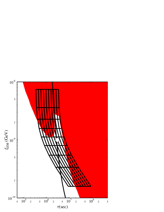
Figure 1: Lifetime $\tau$ and energy release $\xi_{EM}$ in stau decay for $m_{\tilde{\tau}}$ from $300GeV$ to $3TeV$ (from right to left) and $x_{Q}$ from $0.1$ to $0.9$ (from top to bottom). We take $c=1$ and $\Lambda=2\times 10^{16}GeV$. The contour of the chemical potential for photon distribution function is $\mu=9\times 10^{-5}$, with the region to the right of it being excluded by CMBpdg . The shaded regions are excluded by BBN databbn . The circle represents the best fit region with $(\tau,\xi_{EM})=(3\times 10^{6}sec,10^{-9}GeV)$bbn .

In Fig. 1, we plot the decay time and energy release for $m_{\tilde{\tau}}$ from $300GeV$ to $3TeV$ and $x_{Q}$ from $0.1$ to $0.9$. The shaded region is excluded by BBN. The best fit point $(\tau,\xi_{EM})=(3\times 10^{6}\text{sec},10^{-9}GeV)$ is covered in the parameter space, which can suppress the level of ⁷Li and make it to be consistent with the observation bbn .

We will not further consider the constraint from BBN on the stau three-body hadronic decayhadr in this work. Compared with the recent analysis given by Feng et. alfeng , we find there is viable parameter space around the best fit point even after imposing the hadronic constraint in our model. Therefore, we get the conclusion that the quintessino dark matter produced by stau decay is a viable dark matter model, which is consistent with the present experimental constraints.

III supersymmetric neutrino-nucleon cross section

Probing for the long lived stau provides an indirect support for our dark matter model. In this section we calculate the inclusive cross section of stau production from the collision of high energy cosmic neutrinos on the earth matter.

The process which we are interested in is

$$\nu+N\to\tilde{l}+\tilde{q}+X\to 2\tilde{\tau}+X^{\prime}\ ,$$ (6)

where $N=\frac{1}{2}(n+p)$ is an isoscalar nucleon, $X$ ($X^{\prime}$) refers to any type of hadrons and leptons. At the parton level the corresponding process is $\nu+q\to\tilde{l}+\tilde{q}$ with the exchanges of the chargino, $\chi^{+}$, or neutralino, $\chi^{0}$ in the $t$-channel, where $q$ stands for the valence and sea quarks. The $\tilde{l}$ and $\tilde{q}$ in Eq. (6) will quickly decay into two NLSPs. For the calculation of the inclusive cross section in (6), we use the automatic Feynman Diagram Calculation package(FDC) wang:fdc96 , which adopts the CTEQ6-DIS parton distribution functioncteq6 for the isoscalar nucleon.

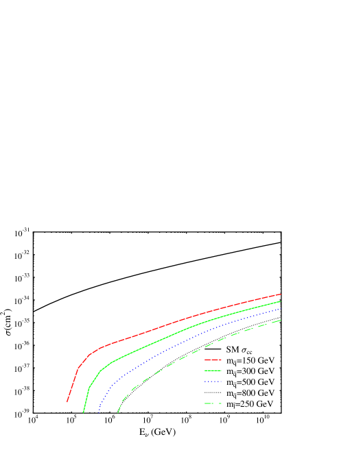
Figure 2: The cross sections of the inclusive process Eq. (6) for $M_{1}=M_{2}=\mu=250GeV$, $m_{\tilde{L}}=m_{\tilde{e_{R}}}=150GeV$, and $m_{\tilde{Q}}=m_{\tilde{u_{R}}}=m_{\tilde{d_{R}}}=150,300,500,800GeV$. The curve with the smallest cross section is for $M_{1}=M_{2}=\mu=400GeV$, $m_{\tilde{L}}=m_{\tilde{e_{R}}}=250GeV$, and $m_{\tilde{Q}}=m_{\tilde{u_{R}}}=m_{\tilde{d_{R}}}=800GeV$. The cross section for the standard model charge current process is also plotted in the figure.

For the soft SUSY breaking terms we take the parameters as $m_{\tilde{L}}=m_{\tilde{e}_{R}}=150GeV$ in the calculations, which gives rise to a lighter stau of about $143GeV$. The gaugino masses and Higgsino mixing parameter are taken as $M_{1}=M_{2}=\mu=250GeV$, so that the neutralinos and charginos are heavier than $\tilde{\tau}$. These parameters give the lightest neutralino mass $m_{\chi^{0}}=181GeV$ and the lighter chargino mass $m_{\chi^{+}}=193GeV$. In Fig. 2, we plot the cross sections for $m_{\tilde{Q}_{L}}=m_{\tilde{q}_{R}}=150,300,500,800GeV$, which are the most sensitive supersymmetric parameters to the cross section. Another set of the soft parameters are taken as $m_{\tilde{L}}=m_{\tilde{e}_{R}}=250GeV$, $M_{1}=M_{2}=\mu=400GeV$ and $m_{\tilde{Q}_{L}}=m_{\tilde{q}_{R}}=800GeV$. (We will denote this set of parameters by $m_{\tilde{l}}=250GeV$ in the text.) In the figure, the inclusive cross section of the charged current process $\nu_{\mu}+N\to\mu+$ anything is also plotted. One can see that the supersymmetric cross section is about 3 orders of magnitude smaller than the standard model one.

IV The distribution of NLSP energy and its range

When the staus propagate in the earth they lose energy through ionization and radiation processes: bremsstrahlung, pair production, and photonuclear interactions. While the energy loss due to ionization is only slowly logarithmically increasing with the energy, the radiation processes cause a loss which in the high energy limit is proportional to the stau energy. The energy loss is usually expressed as

$$-\frac{dE_{\tilde{\tau}}}{dX}=\alpha+\beta E_{\tilde{\tau}}\ ,$$ (7)

where $\alpha$ is due to ionization and $\beta$ is due to radiation. We take $\alpha=2\times 10^{-3}GeVg^{-1}cm^{2}$, which is the same as the ionization loss coefficient of $\mu$ in the rockpdg . Since $\beta$ is proportional to the inverse square of the incident particle mass, we take $\beta=\beta_{\mu}\cdot\left(\frac{m_{\mu}}{m_{\tilde{\tau}}}\right)^{2}$. For $\mu$, $\beta_{\mu}=3.9\times 10^{-6}g^{-1}cm^{2}$pdg . We then obtain the range of the stau with initial energy $E_{0}$

$$R(E_{0})=\frac{1}{\beta}\log\frac{\alpha+\beta E_{0}}{\alpha+\beta m_{\tilde{\tau}}}\ ,$$ (8)

where we have assumed that the energy threshold of the detector can be very small.

The range of the stau is actually a distribution as a function of its energy. For simplicity, we use the range for the average energy of stau, $R(\langle E_{\tilde{\tau}}\rangle)$, in the calculation of the stau flux. Since the collision is through $t$-channel, the stau from the slepton decay and that from the squark decay have very different energies. To discriminate them, we denote them by $\tilde{\tau}_{1}$ and $\tilde{\tau}_{2}$, and the corresponding rang $R_{\tilde{\tau}_{1}}$ and $R_{\tilde{\tau}_{2}}$ respectively.

Figure 3: Angular ($\cos\theta$) and energy distribution of the final particles in the $\nu+N$ CM system, with the beam direction referring to the direction of the incident nucleon. The figures represent the angular distribution of $\tilde{\tau}_{1}$ and $\tilde{\tau}_{2}$ with the beam direction and the energy distributions for $\tilde{\tau}_{1}$, $\tilde{\tau}_{2}$, $l^{\prime}$ respectively and the angle between the two staus. We take the CM energy of $\nu$ and $N$ at 1000 GeV. At higher energies the angular distribution of $\tilde{\tau}_{1,2}$ is more concentrated at $-1$ and the angle between them becomes smaller, while the energy distribution is almost not changed.

For $\tilde{\tau}_{1}$, we assume it has the same energy as the initial slepton, since all the three flavor sleptons have the similar masses. While for $\tilde{\tau}_{2}$, we have to calculate the energy distribution for the process $\tilde{q}\to\tilde{\tau}_{2}+l^{\prime}+q^{\prime}$. In our calculation the energy distributions for the process $\nu+N\to\tilde{\tau}_{1}+\tilde{\tau}_{2}+q^{\prime}+l^{\prime}+X$ are obtained by using the Monte Carlo method to calculate the four-body final state. In Fig. 3 we plot the angular and the energy distribution of the final state particles of the process above in the $\nu+N$ CM system. The angle between the two stau is plotted in the last panel. From the figure we see that the two stau are almost in the same direction as the incident neutrinos. This is easy to be understood since the struck quark carries only small fraction of the total momentum of the nucleon. As the energy increases, the $\tilde{\tau}_{1}$ and $\tilde{\tau}_{2}$ are more concentrated in the forward direction of the incident neutrinos. Therefore, the transverse momentum of the slepton in the CM system is generally much smaller than the momentum of $\nu$ and $N$. Considering that the momentum of the struck quark is widely distributed from just above the threshold to the total momentum carried by the nucleon, we find it is difficult to estimate the transverse momentum of the slepton.

In the $\nu+N$ CM system, the average energy of $\tilde{\tau}_{1}$ changes from $\sim 65\%E_{\nu}^{*}$ to $\sim 75\%E_{\nu}^{*}$, while the average energy of $\tilde{\tau}_{2}$ changes from $\sim 15\%E_{\nu}^{*}$ to $\sim 35\%E_{\nu}^{*}$, both depending not sensitively on the energy of the neutrino, $E_{\nu}^{*}$, and the squark mass. We fix $E_{\tilde{\tau}_{1}}^{*}=70\%E_{\nu}^{*}$, $E_{\tilde{\tau}_{1}}^{*}=20\%E_{\nu}^{*}$ in the CM systerm as a simplification of the calculation. Assuming that the two stau are both in the forward direction, we boost them to the laboratory system. We then get

$$E_{\tilde{\tau}_{1(2)}}^{\text{lab}}\approx\frac{E_{\nu}^{*}}{m_{N}}(E_{\tilde{\tau}}^{*}+|p_{\tilde{\tau}}^{*}|)\approx\frac{2E_{\nu}^{*}}{m_{N}}E_{\tilde{\tau}}^{*}\approx 70\%(20\%)E_{\nu}\ ,$$ (9)

where $E_{\nu}$ is the energy of the primary cosmic neutrinos, and we ignore the $\tilde{\tau}$ mass in the second step, which is a rough approximation at low energies.

V event rate

V.1 Neutrino flux

Waxman and Bahcall (WB) have set an upper bound on the high energy diffuse neutrino flux from the observed cosmic ray flux at high energies. Depending on the evolution of the source activity, they gave the limit on muon neutrino and anti-neutrino extra-galactic fluxwb

$$\left(\frac{d\phi_{\nu}}{dE}\right)_{\text{WB}}=(1\sim 4)\times 10^{-8}\cdot\left(\frac{1GeV}{E}\right)^{2}GeV^{-1}cm^{-2}s^{-1}sr^{-1}\ .$$ (10)

If “unknown source” of protons is taken into account, the low energy neutrino flux can be raised as $d\phi_{\nu}/dE\propto E^{-2}[1+0.1((10^{8}GeV)/E)]$wb . However, the neutrino flux at the energies below about $\sim 10^{6}GeV$ is bounded by AMANDA experimentamanda , i.e., $d\phi_{\nu}/dE\leq 8.4\times 10^{-7}E^{-2}GeVcm^{-2}s^{-1}sr^{-1}$. We refer to the maximal value of flux (10) as ‘WB1’ flux, while the flux raised at low energies and bounded by AMANDA experiment below $\sim 10^{6}GeV$ as the ‘WB2’ flux.

The WB bound holds for the optically thin neutrino sources. Mannheim, Protheroe and Rache (MPR) extend the calculation to “optically thick” sources to the nucleonsmpr . They give an upper bound of diffuse neutrino flux which is almost 30 times larger than the WB1 limit in Eq. (10).

When the extra-galactic neutrinos propagate to the earth, we expect they contain the three flavor neutrinos in ratio of 1:1:1 due to the neutrino oscillation. The supersymmetric particle production rate should be independent of the neutrino flavor since we take all the sleptons almost degenerate. Therefore the three flavors of neutrinos should contribute with the same signal rate, except that $\bar{\nu}_{e}$ has more strongly scattering effect with the earth electron. Here, we calculate the supersymmetric particle signals at the detector contributed by the $\nu_{\mu}+\bar{\nu}_{\mu}$ flux with WB1, WB2 and MPR limit.

V.2 Calculation

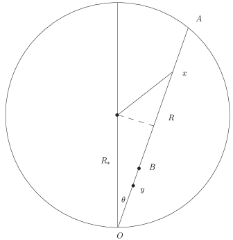
Figure 4: The path of neutrino flux penetrates the earth to the detector at the angle $\theta$.

The earth becomes opaque for neutrinos above about $40TeV$ from the nadir due to the charged-current interaction between neutrino and nucleon. Therefore the scattering of $\nu_{\mu}$ to $\mu$ has to be taken into account.

In Fig. 4 we show the path of a neutrino flux penetrating the earth before it reaches the detector located at the point $O$. We assume that the primary flux at the point $A$ is $\phi_{\nu_{0}}$, then the flux at the point $x$ is given by

$$\phi_{\nu}(x)=\phi_{\nu_{0}}e^{-\int_{A}^{x}n(r)\sigma_{\mu}dR}\ ,$$ (11)

where the integration is along the path from the point $A$ to $x$, with $n(r)$ the nucleon number density, $\sigma_{\mu}$ the standard model charged-current cross section and $R$ is between $0$ and $2R_{*}\cos\theta$, with $R_{*}=6371$ km being the radius of the earth. The number density $n(r)$ is given by $n(r)=\rho(r)N_{A}$, where $\rho(r)$ is the density profile of the earth given in Ref. gandhi and $N_{A}$ is the Avogadro’s number.

Assuming the stau produced below the point $B$ can reach the detector, we then get the flux of stau at the detector $O$

$$\phi_{\tilde{\tau}} = \int_{B}^{O}\phi_{\nu}(B)e^{-\int_{B}^{y}n(r)\sigma_{\mu}dR}\sigma_{\tilde{\tau}}n(r)dy$$ (12)

$$= \phi_{\nu}(B)\frac{\sigma_{\tilde{\tau}}}{\sigma_{\mu}}\left(1-e^{-N_{A}\sigma_{\mu}R_{\tilde{\tau}}}\right)\ ,$$

where both integration are along the path and $\sigma_{\tilde{\tau}}$ is the supersymmetric cross section. It should be noted that at the point corresponding to $R_{\tilde{\tau}_{1}}$ there is only one stau finally arriving at the point $O$, while at the point corresponding to $R_{\tilde{\tau}_{2}}$, there can be two stau arriving at the point $O$.

At large angles, the range of the stau may be larger than the actual depth of the earth that a neutrino has penetrated. In this case we take the actual depth the neutrino penetrated to calculate the probability that a stau can be produced by a neutrino.

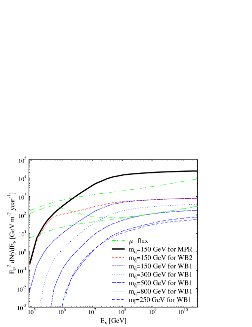
Figure 5: Flux $E_{\nu}^{2}{d\phi_{\tilde{l}}}/{dE_{\nu}}$ as a function of the incident neutrino energy for WB1, WB2 and MPR neutrino fluxes and $m_{\tilde{q}}=150,300,500,800GeV$. The flux for the set of soft parameters with $m_{\tilde{l}}=250GeV$ is also plotted. Similar quantity for $\mu$ flux is plotted in figure. The three curves for $\mu$ flux calculated for the MPR, WB2 and WB1 neutrino fluxes respectively are shown from the top to the bottom.

In Fig. 5, we plot the flux $E_{\nu}^{2}{d\phi_{\tilde{l}}}/{dE_{\nu}}$ as a function of the incident neutrino energy for WB1, WB2 and MPR neutrino fluxes and for $m_{\tilde{q}}=150,300,500,800GeV$. For $m_{\tilde{q}}=150GeV$ we show the results of WB1, WB2 and MPR fluxes. For other parameters we plot only the result of WB1 in the figure for clarity. We notice that the curves become almost flat at the energy above $\sim 10^{8}GeV$. The reason is that for the energies above $\sim 10^{8}GeV$ the range of $\tilde{\tau}$ is so large that it is comparable with the radius of the earth. Therefore in most directions the $\phi_{\tilde{\tau}}$ is proportional to the primary neutrino flux according to Eq. (12), i.e., $\phi_{\nu}(B)=\phi_{\nu_{0}}$ for $R_{\tilde{\tau}}>R(\theta)$.

Note that the contribution to the total $\tilde{\tau}$ events comes mainly from the low energy neutrino flux. (That will be very clear in a $dN_{\tilde{l}}/dE_{\nu}-E_{\nu}$ figure.) The reason is that the neutrino flux decreases with energy with the power law index of $-2$, while the supersymmetric cross section increases with energy (well above the threshold) with a smaller power law index of only about $0.4$.

The corresponding curves for the $\mu$ flux is also plotted in the figure for the WB1, WB2, and MPR neutrino fluxes. It is quite noticeable that the stau flux is even comparable with the $\mu$ flux in the case of $m_{\tilde{q}}=150GeV$.

	$\mu$	($m_{\tilde{q}}=$) $150GeV$	$300GeV$	$500GeV$	$800GeV$	$m_{\tilde{l}}=250GeV$
WB1	$1.8\times 10^{-4}$	$6.6\times 10^{-5}$	$1.5\times 10^{-5}$	$3.3\times 10^{-6}$	$6.5\times 10^{-7}$	$5.8\times 10^{-7}$
WB2	$3.2\times 10^{-3}$	$3.7\times 10^{-4}$	$4.9\times 10^{-5}$	$7.0\times 10^{-6}$	$1.0\times 10^{-6}$	$9.4\times 10^{-7}$
MPR	$5.4\times 10^{-3}$	$2.\times 10^{-3}$	$4.4\times 10^{-4}$	$1.0\times 10^{-4}$	$1.9\times 10^{-5}$	$1.7\times 10^{-5}$

Table 1: Event rate of stau at the detector for per year per $m^{2}$.

Finally, the total event rate for one year is given by

$$\text{event rate}=1\text{year}\cdot 2\pi\int\phi_{\tilde{\tau}}dE_{\nu}d\cos\theta\ .$$ (13)

In table 1, we give the event rates per year per $m^{2}$ for the WB1, WB2 and MPR fluxes for different squark masses. The total $\mu$ events per year per $m^{2}$ is also given in the table. It is quite interesting to notice that even in the most conservative case we may observe one such a event at a detector with $1km^{2}$ effective area per year.

VI conclusion

In this paper we have considered the phenomenology of the model with quintessino as the lightest supersymmetric particle and the dark matter candidatequintessino . In this scenario there exists a long-lived charged heavy particle, usually the lighter $\tilde{\tau}$. It is quite possible to detect such particles in cosmic ray detectors with large effective area. Discovery of the supersymmetric particles of cosmic source will be a valuable complementary for supersymmetry search at high energy colliders.

- (1) Xiao-Jun Bi, Mingzhe Li and Xinmin Zhang, Phys. Rev. D69, 123521 (2004), hep-ph/0308218.
- (2) S. M. Carroll, Phys. Rev. Lett. 81, 3067 (1998).
- (3) M. Li, X. Wang, B. Feng, X. Zhang, Phys. Rev. D65, 103511 (2002); M. Li, X. Zhang, Phys. Lett. B 573, 20 (2003).
- (4) R. H. Cyburt, J.R. Ellis, B.D. Fields, K. A. Olive, Phys. Rev. D67, 103521 (2003).
- (5) J. L. Feng, A. Rajaraman and F. Takayama, Phys. Rev. Lett. 91 (2003) 011302 (2003); Phys. Rev. D 68 (2003) 063504.
- (6) W. B. Lin, D. H. Huang, X. Zhang, and R. Brandenberger, Phys. Rev. Lett. 86, 954 (2001); P. Bode, J. P. Ostriker, and N. Turok, Astrophys. J. 556, 93 (2001).
- (7) W. Buchmuller, K. Hamaguchi, M. Ratz, T. Yanagida, Phys. Lett. B588, 90 (2004); J. L. Feng, A. Rajaraman, F. Takayama, hep-th/0405248; K. Hamaguchi, Y. Kuno, T. Nakaya, M. M. Nojiri hep-ph/0409248; J. L. Feng, B. T. Smith, hep-ph/0409278.
- (8) Xiaojun Bi, Jianxiong Wang and Xinmin Zhang, in preparation.
- (9) O. Adriani, et al., Nucl. Instrum. Methods A 488 (2002) 209.
- (10) Y. Fukuda et al., [Super-Kamiokande Collaboration], Phys. Lett. B 433 (1998) 9.
- (11) J. Ahrens et al., Nucl. Phys. Proc. Suppl. 118 (2003) 388; J. A. Aguilar et al., [The ANTARES Collaboration], astro-ph/0310130; P. K. F. Grieder, [NESTOR Collaboration], Nuovo Cim. 24C (2001) 771.
- (12) I. Albuquerque, G. Burdman, Z. Chacko, hep-ph/0312197.
- (13) R. H. Cyburt, J. Ellis, B. D. Fields and K. A. Olive, Phys. Rev. D 67, 103521 (2003).
- (14) D. J. Fixsen et al, Astrophys. J. 473, 576 (1996).
- (15) K. Hagiwara et al. [Particle Data Group Collaboration], Phys. Rev. D 66 (2002) 010001.
- (16) M. Kawasaki, K. Kohri, T. Moroi, astro-ph/0402490.
- (17) J. L. Feng, S. Su, F. Takayama, hep-ph/0404198; hep-ph/0404231.
- (18) Laura Covi, Hang Bae Kim, Jihn E. Kim, Leszek Roszkowski, JHEP 0105 (2001) 033; Laura Covi, Jihn E. Kim, Leszek Roszkowski, Phys. Rev. Lett. 82 (1999) 4180.
- (19) J. X. Wang, “New computing techniques in physics research III”, 517-522, Proceeding of AI93, Oberamergau, Germany; Program and descriptions of FDC can be found at the web page http://www.ihep.ac.cn/lunwen/wjx//index.html.
- (20) J. Pumplin, D.R. Stump, J.Huston, H.L. Lai, P. Nadolsky, W.K. Tung, JHEP 0207 (2002) 012; D. Stump, J. Huston, J. Pumplin, W.K. Tung, H.L. Lai, S. Kuhlmann, J. Owens, JHEP 0310 (2003) 046.
- (21) E. Waxman and J. Bahcall, Phys. Rev. D59 (1998) 023002; J. Bahcall and E. Waxman, Phys. Rev. D64 (2001) 023002.
- (22) J. Ahrens et al. (AMANDA collaboration), Phys. Rev. Lett. 90 (2003) 251101.
- (23) K. Mannheim, R. J. Protheroe and J. P. Rache, Phys. Rev. D63 (2001) 023003.
- (24) R. Gandhi, C. Quigg, M. H. Reno and I. Sarcevic, Astropart. Phys. 5 (1996) 81.