Probing the Planck Scale with Proton Decay
 

Abstract

We advocate the idea that proton decay may probe physics at the Planck scale instead of the GUT scale. This is possible because supersymmetric theories have dimension-5 operators that can induce proton decay at dangerous rates, even with $R$-parity conservation. These operators are expected to be suppressed by the same physics that explains the fermion masses and mixings. We present a thorough analysis of nucleon partial lifetimes in models with a string-inspired anomalous $U(1)_{X}$ family symmetry which is responsible for the fermionic mass spectrum as well as forbidding $R$-parity violating interactions. Protons and neutrons can decay via $R$-parity conserving non-renormalizable superpotential terms that are suppressed by the Planck scale and powers of the Cabibbo angle. Many of the models naturally lead to nucleon decay near present limits without any reference to grand unification.

I Introduction

Baryon number is an accidental symmetry of the Standard Model (SM). However, it is unlikely that baryon number will remain a symmetry up to the highest energy scales. Because of the gauge hierarchy problem it is strongly believed that the SM must be augmented by new physics at the TeV scale. There is no theoretical reason to believe that such new physics will still conserve $U(1)_{B}$. In fact, baryon number violation is one of the necessary ingredients in models that explain the matter-antimatter asymmetry in the universe Sakharov:dj . We therefore expect $U(1)_{B}$ to be violated at some higher energy scale. Current and future experiments of nucleon decay may thus be probes of high-scale physics. For example, the partial lifetime of the decay mode $p\to K^{+}\bar{\nu}$ is greater than $1.6\times 10^{33}$ years Kearns , which places stringent constraints on scenarios of new physics.

On the other hand, supersymmetry is considered the leading candidate for physics beyond the SM because it solves the gauge hierarchy problem once and for all and it is also consistent with grand unified theories (GUTs). It is often said that since quarks and leptons lie in the same GUT multiplets, an observation of proton decay will be a signal of a GUT. Indeed, the minimal supersymmetric $SU(5)$ GUT has been excluded because the unification of gauge couplings forces the model into a region of parameter space where the proton decays too quickly Murayama:2001ur .

However, it is an under-publicized fact that supersymmetric models predict proton decay even without unification. Conventionally $R$-parity ($R_{p}$) is imposed as an exact symmetry in order to prevent the proton from decaying through renormalizable operators. But in a generic supersymmetric model one can still write down $R_{p}$-conserving, yet baryon and lepton number violating, $D=5$ operators suppressed by a single power of the cutoff scale, which we take to be the reduced Planck scale $M_{\mathrm{Pl}}\sim 2.4\times 10^{18}$ GeV. These operators come from the superpotential

$$W_{5}=\frac{\epsilon_{abc}}{M_{\mathrm{Pl}}}\left(C^{ijkl}_{L}(Q_{i}^{a}Q_{j}^{b})(Q_{k}^{c}L_{l})+C^{ijkl}_{R}{\,\overline{\!U}{}}_{i}^{a}{\,\overline{\!U}{}}_{j}^{b}{\,\overline{\!D}{}}_{k}^{c}{\,\overline{\!E}{}}_{l}\right).$$ (1)

Here $Q,L$ are quark and lepton doublet superfields and ${\,\overline{\!U}{}},{\,\overline{\!D}{}},{\,\overline{\!E}{}}$ are $SU(2)_{L}$ singlets. The $SU(2)_{L}$ indices are contracted between the terms in parentheses, while $i,j,k,l$ are generational indices and $a,b,c$ are color indices. From an effective field theoretic point of view one expects these operators to appear with coefficients $C_{L}$ and $C_{R}$ of $\mathcal{O}(1)$.

Supersymmetry’s dirty little secret is that if one were to pick generic $\mathcal{O}(1)$ numbers for the coefficients $C_{L}$ and $C_{R}$, the proton lifetime would be about $10^{17}$ years, many orders of magnitude below the experimental limit. Thus the coefficients $C_{L}$ and $C_{R}$ must be highly suppressed in any viable supersymmetric model.

We do not consider this embarrassment a death-blow for supersymmetric models, however. This is because the SM already contains highly suppressed dimensionless numbers, namely the Yukawa coupling constants. It is unsatisfactory to have an effective theory that is valid up to the Planck scale without explaining the origin of small coefficients for $H_{\mathcal{U}}Q_{i}{\,\overline{\!U}{}}_{j}$, $H_{\mathcal{D}}Q_{i}{\,\overline{\!D}{}}_{j}$ and $H_{\mathcal{D}}L_{i}{\,\overline{\!E}{}}_{j}$. Such an explanation should naturally determine the coefficients of $Q_{i}Q_{j}Q_{k}L_{l}$ and ${\,\overline{\!U}{}}_{i}{\,\overline{\!U}{}}_{j}{\,\overline{\!D}{}}_{k}{\,\overline{\!E}{}}_{l}$, likely suppressing them as well Murayama:1994tc . In the context of supersymmetric models the most promising scenario for generating small Yukawa couplings is that of Froggatt and Nielsen Froggatt:1978nt (see Dreiner:2003hw for an exhaustive list of references), for which the suppression of proton decay has been demonstrated Murayama:1994tc ; Kakizaki:2002hs . In Dreiner:2003hw the tight experimental bounds on exotic processes were brought to bear on certain Froggatt-Nielsen models found in the literature. Indeed, many models were found to be incompatible with data solely due to insufficient suppression of $Q_{i}Q_{j}Q_{k}L_{l}$. The relation between the fermion mass hierarchy in the SM and the suppression of proton decay also occurs in other non-supersymmetric models such as Arkani-Hamed:1999dc ; Kakizaki:2001ue .

In order to predict proton decay rates originating from Planck scale $D=5$ operators we have to specify the framework of fermion masses and mixings. We would like the framework to be specific enough so that we can make quantitative predictions, but also general enough so that we can study the generic features of Planck scale proton decay. In this paper we will focus on a recently proposed class of models based on a single, anomalous Froggatt-Nielsen flavor symmetry Dreiner:2003yr . In this class of models the MSSM superfields are charged under a horizontal $U(1)_{X}$ symmetry that is spontaneously broken by the non-zero VEV of a flavon field, $A$. The MSSM Yukawa terms are then suppressed by the ratio $\epsilon=\langle A\rangle/M_{\mathrm{Pl}}$ raised to the the appropriate power necessary to conserve $U(1)_{X}$. The models in Dreiner:2003yr are ambitious:

1. The $U(1)_{X}$ is the only symmetry beyond the SM gauge groups.

2. The only fields charged under the SM gauge groups are those in the MSSM. However, there may be (hidden sector) fields charged only under $U(1)_{X}$.

3. The $U(1)_{X}$ charge assignments and breaking scale are inspired directly from string theory. Anomalies are canceled by the Green-Schwarz mechanism which places sum rules on the $X$-charges.

4. The Cabibbo angle is calculated. It is set by the flavon VEV which is is determined by string theory, yielding the phenomenologically interesting value $\epsilon=\langle A\rangle/M_{\mathrm{Pl}}=0.17$–0.22.

5. The charge assignments are chosen to yield the measured quark and lepton masses, including CKM mixing.

6. Neutrino mixings are also a result of the charge assignments.

7. $R$-parity is an exact (accidental) symmetry of the $U(1)_{X}$ charge assignments, preventing tree-level nucleon decay.

That these seven goals can be achieved within a single, simple framework is non-trivial and encouraging. As was shown in Dreiner:2003yr , there is only a finite number of $X$-charge assignments with these properties. It is very interesting that the predicted nucleon partial lifetimes in these models are generically within a few orders of magnitude of the current limits of about $10^{32}$ years. This already rules out some specific charge assignments, and means that others will be directly tested very soon. It is important to note that in general these models do not have GUT-compatible $X$-charges, but they nonetheless lead to very interesting nucleon decay rates not much smaller than those predicted by GUTs.

In this paper we systematically explore the nucleon partial lifetimes predicted by the $U(1)_{X}$ Froggatt-Nielsen models presented in Dreiner:2003yr . In Section II we briefly review these models, then in Section III we do some quick estimates of the lifetimes. In Section IV we describe our method of computing the nucleon decay rates. Section V contains our main results, namely that the $U(1)_{X}$ models of flavor are already constrained by current nucleon decay data, and they will continue to be tested by future experiments. Our conclusions are presented in Section VI, while Appendix A carefully explains the dressing diagrams relevant for our analysis, and Appendix B discusses the effects of canonicalizing the Kähler potential and transforming from the interaction basis into the mass basis.

II Froggatt-Nielsen Framework

We will analyze the class of Froggatt-Nielsen models presented in Dreiner:2003yr . In this section we summarize the results that are relevant for our analysis and refer readers to that paper for details. Below the reduced Planck scale the gauge group and particle content are those of the MSSM, with the addition of two right-handed neutrinos, a single flavon superfield $A$, and a generation-dependent $U(1)_{X}$ gauge group with anomalies canceled by the Green-Schwarz mechanism Green:sg . Since all matter fields are charged under $U(1)_{X}$, their couplings to the flavon are determined by $U(1)_{X}$ invariance. The goal is to have the flavon couplings generate the generation dependent masses and mixings in the fermion spectrum.

For example, masses for the up-type quarks originate from the non-renormalizable operator

$${g_{U}}^{ij}~{}\bigg{(}\frac{A}{M_{\mathrm{Pl}}}\bigg{)}^{{X_{H_{\mathcal{U}}}+X_{Q_{i}}+X_{\overline{U}_{j}}}}H_{\mathcal{U}}\,Q_{i}\,\overline{U}_{j},$$ (2)

where the flavon charge is defined to be $X_{A}=-1$ and ${g_{U}}^{ij}$ are $\mathcal{O}(1)$ coefficients that are undetermined within the effective theory below $M_{\mathrm{Pl}}$. The dimensionless ${g_{U}}^{ij}$ is zero if $X_{H_{\mathcal{U}}}+X_{Q_{i}}+X_{\overline{U}_{j}}$ is negative or fractional. The powers of $A$ in Eqn. (2) compensate the $U(1)_{X}$ charges of $H_{\mathcal{U}}\,Q_{i}\,\overline{U}_{j}$ yielding $U(1)_{X}$ gauge invariants. The Dine-Seiberg-Wen-Witten-generated Fayet-Iliopoulos term for $U(1)_{X}$ induces a VEV for the scalar component of the flavon field Dine:bq ; Dine:1986zy ; Atick:1987gy ; Dine:1987gj . The VEV is given by $\langle A\rangle=\epsilon M_{\mathrm{Pl}}$, where $\epsilon$ naturally turns out to be the size of the sine of the Cabibbo angle, $\epsilon\sim 0.2$. After $U(1)_{X}$-breaking one gets the Yukawa couplings

$${G_{\!U}}^{ij}~{}=~{}{g_{U}}^{ij}~{}\epsilon^{X_{H_{\mathcal{U}}}+X_{Q_{i}}+X_{\overline{U}_{j}}},$$ (3)

which are suppressed by powers of $\epsilon$. In this way the charge assignments of the MSSM matter fields determine the fermion mass hierarchy. Once the $X$-charges are chosen to reproduce the mass spectrum, the $\epsilon$-suppressions of other superpotential terms are determined up to $\mathcal{O}(1)$ coefficients, with higher-dimensional operators like $Q_{i}Q_{j}Q_{k}L_{l}$ being suppressed by additional powers of $M_{\mathrm{Pl}}$. It is this connection that we will be exploiting to estimate the nucleon decay lifetimes within this Froggatt-Nielsen framework.

The $X$-charges are determined by requiring cancellation of chiral anomalies between $U(1)_{X}$ and the SM gauge group, prohibition of all $R_{p}$-violating interactions, and generation of the phenomenologically viable fermion masses and the CKM matrix. The $X$-charges of the MSSM superfields are then specified by six integer parameters, as demonstrated in Dreiner:2003yr and displayed in their Table 2. These $X$-charges are further constrained by the phenomenology of neutrino mixing, which fixes two of those six parameters . The $X$-charge of each superfield is determined by the four remaining parameters, $x,y,z$ and $\Delta^{\!H}$, and is shown in Table 1. The physical significance of these parameters will be explained below.

$~{}~{}~{}\phantom{\Big{|}}X_{H_{\mathcal{D}}}$	$=$	$\frac{-24+12y+z(9+4z)+x(4x+22+6z)-2\Delta^{\!H}(2x+12+3z)}{10~{}(6+x+z)}$
$~{}\phantom{\Big{|}}X_{H_{\mathcal{U}}}$	$=$	$-z-\phantom{\Big{|}}X_{H_{\mathcal{D}}}$
$~{}\phantom{\Big{|}}X_{Q^{1}}$	$=$	$\frac{1}{3}\Big{(}\frac{19}{2}-X_{H_{\mathcal{D}}}+x+2y+2z-\Delta^{\!H}\Big{)}$
$~{}\phantom{\Big{|}}X_{Q_{2}}$	$=$	$X_{Q^{1}}-1-y$
$~{}\phantom{\Big{|}}X_{Q_{3}}$	$=$	$X_{Q^{1}}-3-y$
$~{}\phantom{\Big{|}}X_{\overline{D}_{1}}$	$=$	$-X_{H_{\mathcal{D}}}-X_{Q_{1}}+4+x$
$~{}\phantom{\Big{|}}X_{\overline{D}_{2}}$	$=$	$X_{\overline{D}_{3}}=X_{\overline{D}_{1}}-1+y$
$~{}\phantom{\Big{|}}X_{\overline{U}_{1}}$	$=$	$X_{H^{\mathcal{D}}}-X_{Q_{1}}+8+z$
$~{}\phantom{\Big{|}}X_{\overline{U}_{2}}$	$=$	$X_{\overline{U}_{1}}-3+y$
$~{}\phantom{\Big{|}}X_{\overline{U}_{3}}$	$=$	$X_{\overline{U}_{1}}-5+y$
$~{}\phantom{\Big{|}}X_{L_{1}}$	$=$	$\frac{1}{2}+X_{H_{\mathcal{D}}}+\Delta^{\!H}$
$~{}\phantom{\Big{|}}X_{L_{2}}$	$=$	$X_{L_{3}}=X_{L_{1}}-z$
$~{}\phantom{\Big{|}}X_{\overline{E}_{1}}$	$=$	$-X_{H_{\mathcal{D}}}{+~{}4}-X_{L_{1}}+x+z$
$~{}\phantom{\Big{|}}X_{\overline{E}_{2}}$	$=$	$-X_{H_{\mathcal{D}}}{+~{}2}-X_{L_{1}}+x+z$
$~{}\phantom{\Big{|}}X_{\overline{E}_{3}}$	$=$	$-X_{H_{\mathcal{D}}}\phantom{+~{}4}-X_{L_{1}}+x+z$

Table 1: $R_{p}$-conserving $X$-charge assignments of the MSSM superfields in terms of four parameters: $x$, $y$, $z$, $\Delta^{H}$. The charge assignments are as in Table 2 of Dreiner:2003yr with their $\zeta$ and $\Delta^{L}_{31}$ both taken to be $-z$ as required by neutrino mixing phenomenology.

Only the three parameters $x$, $y$ and $z$ are relevant for nucleon decay. They are restricted to a small set of integers, which leads to 24 distinct models with different nucleon decay signatures. The allowed values are $x=0$, $1$, $2$, $3$; $y=-1$, $0$, $1$, and $z=0$, $1$.

The parameter $x$ is related to the ratio of the bottom and top quark masses, and is thus also connected to $\tan\beta$,

$$\frac{m_{b}}{m_{t}}\sim\frac{\epsilon^{x}}{\tan\beta}.$$ (4)

Since $\epsilon\sim 0.2$, larger $x$ corresponds to smaller $\tan\beta$, but because of unknown $\mathcal{O}(1)$ coefficients, we cannot determine $\tan\beta$ exactly. To simplify our analysis we will choose a specific, reasonable value of $\tan\beta$ for each value of $x$, namely $\tan\beta=50$, $20$, $5$, $3$ for $x=0,1,2,3$, respectively.

The three choices for the parameter $y$ determine the texture of the up- and down-quark Yukawa matrices and therefore also the CKM matrix. One finds

$$y=-1:~{} \boldsymbol{V_{\!C\!K\!M}}\sim\left(\begin{array}[]{ccc}1&1&\epsilon^{2}\\ 1&1&\epsilon^{2}\\ \epsilon^{2}&\epsilon^{2}&1\end{array}\right),$$ (8)

$$y=0:~{} \boldsymbol{V_{\!C\!K\!M}}\sim\left(\begin{array}[]{ccc}1&\epsilon&\epsilon^{3}\\ \epsilon&1&\epsilon^{2}\\ \epsilon^{3}&\epsilon^{2}&1\end{array}\right),$$ (12)

$$y=1:~{} \boldsymbol{V_{\!C\!K\!M}}\sim\left(\begin{array}[]{ccc}1&\epsilon^{2}&\epsilon^{4}\\ \epsilon^{2}&1&\epsilon^{2}\\ \epsilon^{4}&\epsilon^{2}&1\end{array}\right).$$ (16)

Finally, the parameter $z$ is related to the charged lepton mass spectrum,

$$\frac{m_{e}}{m_{\mu}}\sim\epsilon^{2+z}.$$ (17)

In combination with neutrino phenomenology and the requirement that $R_{p}$ is conserved by virtue of the $X$-charges, it turns out that $z$ specifies the texture of the MNS matrix:

$$\boldsymbol{U_{\!M\!N\!S}}\sim\left(\begin{array}[]{ccc}1&\epsilon^{z}&\epsilon^{z}\\ \epsilon^{z}&1&1\\ \epsilon^{z}&1&1\end{array}\right).$$ (18)

Here we see that $z=0$ corresponds to an “anarchical” MNS matrix Hall:1999sn ; Haba:2000be , whereas $z=1$ corresponds to a “semi-anarchical” MNS matrix Sato:1997hv .

The minimalist approach is to add only two right-handed neutrinos. When this approach is taken the fourth parameter, $\Delta^{\!H}$, can take two different values for each set of $\{x,y,z\}$, but it has no impact on nucleon lifetimes and so it is irrelevant for our purposes. However, our analysis does not depend on the number of right handed neutrinos.

In addition to specifying the CKM and MNS textures, the parameters $\{x,y,z\}$ also have bearing on other aspects of the UV physics. For example, $SU(5)$ invariance is only consistent with $y=1$ and $z=0$. Also, $z=1$ prohibits the operator $H_{\mathcal{D}}H_{\mathcal{U}}$, thus allowing the $\mu$-term to be generated by the Giudice-Masiero mechanism Giudice:1988yz ; Kim:1994eu . If one has a preference towards a specific physical scenario, the number of models to choose from is significantly reduced. For example, the models in Dreiner:2003yr were chosen to have $z=1$ for the sake of a natural $\mu$-parameter, $y=0$ to obtain the most natural CKM matrix, and $x=2,3$ to avoid proton decay limits.

Other criteria may be used in choosing one’s favorite model. For instance, the values of the $X$-charges are much more aesthetically pleasing in some models than others. For example, taking $x=2$, $y=1$, $z=0$ and $\Delta^{\!H}=9$, one finds the $X$-charges of all MSSM superfields are integers or half-odd-integers, as shown in Table 2. However, in this paper we will treat all 24 distinct models equally and focus only on their predictions for nucleon decay.

Generation $i\phantom{\Big{|}}$	1	2	3
$\phantom{\Big{|}}X_{Q_{i}}\phantom{\Big{|}}$	$5/2$	$1/2$	$-3/2$
$\phantom{\Big{|}}X_{L_{i}}\phantom{\Big{|}}$	$13/2$	$13/2$	$13/2$
$\phantom{\Big{|}}X_{{\,\overline{\!U}{}}_{i}}\phantom{\Big{|}}$	$5/2$	$1/2$	$-3/2$
$\phantom{\Big{|}}X_{{\,\overline{\!D}{}}_{i}}\phantom{\Big{|}}$	$13/2$	$13/2$	$13/2$
$\phantom{\Big{|}}X_{{\,\overline{\!E}{}}_{i}}\phantom{\Big{|}}$	$5/2$	$1/2$	$-3/2$

$\phantom{\Big{|}}X_{H_{\mathcal{D}}}=-3$, $X_{H_{\mathcal{U}}}=3\phantom{\Big{|}}$

Table 2: An example of an $X$-charge assignment for the matter superfields in the model with $x=2$, $y=1$, $z=0$, and $\Delta^{\!H}=9$. $\Delta^{\!H}$ helps to determine the specific charges, but its effects cancel out in all the nucleon decay operators.

III Quick Estimates

A quick estimate shows that the operator $Q_{1}Q_{1}Q_{2}L_{3}$ leads a proton lifetime of $\sim 10^{17}\epsilon^{-2n}$ years, where $n=9+x+y+z$ is the sum of the $X$-charges for the four superfields. Since $\epsilon\sim 0.2$, we need to have $n\gtrsim 11$ to satisfy the experimental limit of about $10^{33}$ years for $p\to K^{+}\bar{\nu}_{\tau}$. This demonstrates the general trend that larger values of $x$, $y$, and $z$ will lead to greater suppression of the decay rate and hence a longer lifetime.

It turns out that the nucleon lifetimes predicted by our Froggatt-Nielsen model are in the same ballpark as those predicted by GUT models. This can be understood relatively easily. For the operator $Q_{2}Q_{2}Q_{1}L_{2}$ we can rewrite the suppression in terms of Yukawa couplings (ignoring $\mathcal{O}(1)$ factors),

$$\frac{1}{M_{\mathrm{Pl}}}\epsilon^{8+x+z}=\frac{\epsilon}{M_{\mathrm{Pl}}}\epsilon^{z}\epsilon^{4}\epsilon^{2+x}\epsilon=\frac{\epsilon}{M_{\mathrm{Pl}}}\frac{\mu}{m_{3/2}}{G_{\!U}}^{22}~{}{G_{\!E}}^{22}\epsilon,$$ (19)

where we have used the phenomenological constraints on the $X$-charges from Section 5 in Dreiner:2003yr to identify the Yukawa couplings. This is to be compared with the coefficient of the same operator coming from an $SU(5)$ GUT theory, which is

$$\frac{1}{M_{\mathrm{GUT}}}{G_{\!U}}^{22}~{}{G_{\!E}}^{22}\lambda_{C}.$$ (20)

Equating $\epsilon$ with $\lambda_{C}$ and noting that the $\mu$-parameter cannot be too different from the gravitino mass, the difference between the coefficients is simply $\lambda_{C}(M_{\mathrm{GUT}}/M_{\mathrm{Pl}})$. Considering the fact that these two models involve completely different physics, we find this difference interestingly small. The estimation above is obviously very crude and calls for a more rigorous analysis which is the goal of this work.

IV Nucleon Decay Computations

In this section we describe our calculations of the various nucleon decay modes. We use the standard methods for the computations, following Murayama:1994tc and Goto:1998qg . The starting point is the higher-dimensional UV Lagrangian shown in Eqn. (1). The dimension-five fermion-fermion-scalar-scalar terms arising from these operators can be “dressed”, whereby the scalars exchange a gaugino or higgsino and are converted into fermions, as shown in Figure 1. Below the scale of the soft masses they become four-fermion operators and contribute to nucleon decay. The matrix elements of these operators can be evaluated using the well-known chiral Lagrangian technique Claudson:1981gh .

Figure 1: An example of a dimension-5 operator that can be dressed by neutral or charged winos and higgsinos.

The quark doublet superfields $Q$ in Eqn. (1) are taken to be in the SuperCKM basis, namely $Q=(U,D^{\prime})=(U,V_{\!C\!K\!M}D)$ where $U$ and $D$ are the mass eigenstates. Thus the couplings to the mass eigenstate quark operators will come with various CKM factors. However, we cannot necessarily neglect operators with small CKM factors because they may be offset by the lesser degree of $\epsilon$-suppression in $C^{ijkl}_{L,R}$. In other words, operators $Q_{i}Q_{j}Q_{k}L_{l}$ containing third generation quarks will have small CKM couplings to the first generation quarks in the nucleon, but will have correspondingly larger coefficients $C^{ijkl}_{L,R}$ due to the $X$-charge assignments for the third generation.

Note that the $U(1)_{X}$ basis is not necessarily the same as the SuperCKM basis nor the mass eigenbasis. Thus it is important to take these various changes of basis into consideration when determining the $\epsilon$-suppression of the nucleon decay operators. For the most part this only effects the $\mathcal{O}(1)$ coefficients, which we are ignorant of anyway. Nevertheless, we have performed a thorough analysis of this effect as described in Appendix B.

The operators $Q_{i}Q_{j}Q_{k}L_{l}$ and ${\,\overline{\!U}{}}_{i}{\,\overline{\!U}{}}_{j}{\,\overline{\!D}{}}_{k}{\,\overline{\!E}{}}_{l}$ are not all independent. Fierz identities may be used to convert all of the operators into a smaller set which we choose as our basis of independent operators. One can further reduce the number of operators in this set by noting that contributions to nucleon decay can only come from operators with at least one first-generation superfield. The Fierz identities and a list of independent operators are given in Appendix A. Since we do not know the exact coefficients in front of these operators, we will assume that in the UV all of the operators in our basis are generated and that their unknown coefficients are given by the $\epsilon$-suppression determined by the $X$-charges and $\mathcal{O}(1)$ numerical factors.

As argued above, the $\epsilon$-suppression is essential for the predicted nucleon lifetimes to be above the current limits. This suppression is determined by the $X$-charges of $Q_{i}$, ${\,\overline{\!U}{}}_{i}$, ${\,\overline{\!D}{}}_{i}$, $L_{i}$ and ${\,\overline{\!E}{}}_{i}$, which are in turn determined by the choice of the model parameters $x$, $y$, and $z$. Note that $\epsilon$ itself also has mild dependence on the model parameters,

$$\epsilon~{}=~{}\frac{g_{3}}{4\pi\sqrt{2}}\sqrt{3(6+x+z)}\,$$ (21)

where the QCD gauge coupling $g_{3}$ is roughly $0.72$ at high energies. The dependence of the $\epsilon$-suppression on the choice of $X$-charges leads to the different patterns of nucleon partial lifetimes that we study in the next section.

Renormalization group effects enhance the nucleon decay operators due to running between $M_{\mathrm{Pl}}$ and $m_{p}$. For simplicity, we compute the supersymmetric running from $M_{\mathrm{Pl}}$ down to $m_{Z}$ from the gauge couplings, ignoring corrections proportional to Yukawa couplings. The left- and right-handed operators, $Q_{i}Q_{j}Q_{k}L_{l}$ and ${\,\overline{\!U}{}}_{i}{\,\overline{\!U}{}}_{j}{\,\overline{\!D}{}}_{k}{\,\overline{\!E}{}}_{l}$, are enhanced by a factor

$$\left(\frac{\alpha_{1}(M_{\mathrm{Pl}})}{\alpha_{1}(m_{Z})}\right)^{c_{1}}\left(\frac{\alpha_{2}(M_{\mathrm{Pl}})}{\alpha_{2}(m_{Z})}\right)^{c_{2}}\left(\frac{\alpha_{3}(M_{\mathrm{Pl}})}{\alpha_{3}(m_{Z})}\right)^{c_{3}}.$$ (22)

Here ${\alpha_{i}}^{-1}(q)={\alpha_{i}}^{-1}(m_{Z})-\frac{b_{i}}{2\pi}\ln\left(q/m_{Z}\right)$ with $b_{i}=(33/5,1,-3)$ and $c_{i}=(1/33,3,-4/3)$ for LH and $(2/11,0,-4/3)$ for RH operators. Also, $g_{1}^{2}=(5/3)g^{\prime 2}$ Numerically this enhances the LH operators by a factor of $9.3$ and the RH operators by a factor of $5.6$.

In general there are many different ways the dimension-five operators can be dressed to give four-fermion operators. In our scenario we assume that supersymmetry breaking is sufficiently flavor blind so that the flavor mixing in gluino-quark-squark vertices is negligible. Then in the limit of degenerate squarks and degenerate sleptons the contributions from gluino dressing cancel due to a Fierz identity, as explained in more detail in Appendix A. There it is also shown that bino dressing does not contribute to nucleon decay. All contributions from neutral-higgsino dressing are extremely suppressed by small, first-generation Yukawa couplings, so we ignore them. We do include the leading contributions from charged-higgsino dressing. In the case of charged-lepton decay modes these contributions turn out to be negligible, but Goto:1998qg has shown that they can be important for the antineutrino decay modes. The bulk of the contributions come from charged-wino dressing, though the neutral-wino dressing can be comparable for the antineutrino decay modes.

The dressing leads to a four-fermion vertex which must then be run from the scale of the soft masses, roughly $10^{2}$ GeV, down to $1$ GeV where they mediate nucleon decay. For simplicity we compute the QCD running only from $m_{Z}$ down to $1$ GeV, which leads to an enhancement given in Buras:1977yy , namely

$$\left(\frac{\alpha_{3}(M_{\mathrm{low}})}{\alpha_{3}(M_{\mathrm{high}})}\right)^{2/\beta_{0}}$$ (23)

where $\beta_{0}=11-\frac{2}{3}f$ and $f$ is the number of quark flavors with masses less than $M_{\mathrm{high}}$. There are three of these enhancement factors for the successive steps between $m_{Z}$, $m_{b}$, $m_{c}$, and $m_{p}$. In each step the QCD coupling is given by ${\alpha_{3}}^{(f)}(q)=4\pi/(\beta_{0}\ln(q^{2}/{\Lambda_{f}}^{2}))$, where $\Lambda_{f}$ is determined by requiring that $\alpha_{3}$ be continuous between successive intervals. Numerically we use $m_{b}=4.2$ GeV, $m_{c}=1.2$ GeV, and $m_{p}=1$ GeV, which gives a total contribution of $1.3$, and is quite insensitive to the exact thresholds for $m_{b}$ and $m_{c}$. Together with the high scale running mentioned above, there is a net enhancement of approximately $12$ for $C_{L}$ and $7$ for $C_{R}$.

The chiral Lagrangian can be used to determine the decay rate induced by the four-fermion operators Claudson:1981gh . The partial decay width of a nucleon $B_{i}$ into a meson $M_{j}$ and lepton $l_{k}$ is given by

$$\Gamma(B_{i}\rightarrow M_{j}l_{k})=\frac{m_{i}}{32\pi~{}f_{\pi}^{2}}\left(1-\frac{{m_{j}}^{2}}{{m_{i}}^{2}}\right)^{\!2}\!\left(\big{|}A^{ijk}_{L}\big{|}^{2}+\big{|}A^{ijk}_{R}\big{|}^{2}\right)$$ (24)

where $A^{ijk}_{L,R}$ can be found in Table 1 of Goto:1998qg , given in terms of the coefficients of the various four-fermion operators generated by dressing of the superpotential operators shown in Eqn. (1). The numerical values of $A_{L,R}$ depend on several input parameters. The coupling between baryons and mesons in the chiral Lagrangian are given by $D$ and $F$. As in Claudson:1981gh we take $D=0.81$, $F=0.44$, and $f_{\pi}=139$ MeV.

Our computations of nucleon lifetimes are subject to two types of uncertainties, those that reflect our current lack of knowledge and those that are inherent to the effective theory framework of our model. The first type includes the uncertainty in the hadronic matrix element and the masses of the superpartners, both of which we assume will be pinned down more precisely by the time the next generation nucleon decay experiments start taking data. The second type includes the unknown $\mathcal{O}(1)$ coefficients that come with the non-renormalizable superpotential operators, which cannot be determined without a full theory of the Planck scale physics. We will discuss each of these uncertainties in turn.

The value of the hadronic matrix element must be evaluated to convert the four-fermion operators into nucleon lifetimes. In the framework of the chiral Lagrangian this appears as two parameters $\beta_{p}$ and $\alpha_{p}$, which are related by $\alpha_{p}=-\beta_{p}$. Unfortunately, the value of $\beta_{p}$ is only known to roughly a factor of 10. The conservative range often taken is $\beta_{p}=0.003$–$0.03$ GeV³. Recently there has been some progress evaluating $\beta_{p}$ on the lattice, yielding the results $\beta_{p}=0.014\pm 0.001$ GeV³ in Kuramashi:2000hw and $\beta_{p}=0.007\pm 0.001$ GeV³ in Aoki:2002ji . Note that the errors are only statistical, and do not reflect systematic effects such as quenching. Since $\beta_{p}$ appears in the amplitude, any uncertainty in its value gets squared in the decay rate or lifetime. However, this uncertainty is common across all modes and all different models, so it simply represents an overall rescaling of the lifetimes. For our computations we will use an intermediate value, $\beta_{p}=0.01$ GeV³. A smaller value of $\beta_{p}$ would give a smaller decay rate and a longer lifetime. Allowing for the range $0.003$–$0.03$ thus corresponds to a change in our results by a factor of 10 in both directions. Again, we can look forward to reduction in the uncertainty in the hadronic matrix element, which will reduce the uncertainty in our computations.

The scale of the superpartner masses is another uncertainty in our computations that will be reduced if supersymmetry is discovered at a collider. The superpartner masses enter through the loop in the dressed diagrams such as the one in Figure 1. We assume that the squarks and sleptons all have a common mass, $m_{\mathrm{soft}}$. If the gaugino (or higgsino) mass is much less than the squark mass, the contribution from the loop is given by $M_{\mathrm{gaugino}}/m_{\mathrm{soft}}^{2}$, whereas if the gauginos are degenerate with the squarks at $m_{\mathrm{soft}}$, then the loop factor is $1/(2m_{\mathrm{soft}})$. One can imagine extremes where all the superpartners are relatively light, near $100$ GeV, leading to the shortest lifetimes, or the opposite extreme where the scalars are heavy (TeV) and the gauginos are light (100 GeV), leading to the longest lifetimes.

We can cover the different possibilities by taking all superpartners to be degenerate at $m_{\mathrm{soft}}$ and then allowing $m_{\mathrm{soft}}$ to range from 100 GeV to 10 TeV. The latter case does not mean the superpartner masses are actually 10 TeV, but rather represents the case where squark and slepton masses are around 1 TeV and wino masses are 100 GeV. In our computations we will choose a middle ground by assuming of $m_{\mathrm{soft}}=1$ TeV. With this assumption, the proton lifetime simply scales inversely with $m_{\mathrm{soft}}^{2}$. Choosing one of the other two scenarios described above would change the nucleon lifetimes by a factor of 100. We reiterate that this uncertainty will disappear once the superpartner spectrum is measured, most likely at the LHC.

Our ignorance of the $\mathcal{O}(1)$ coefficients appearing in front of each operator in Eqn. (1) is an uncertainty inherent in the framework of effective field theory. $A_{L,R}$ in Eqn. (24) are each the sum of several contributing amplitudes from different operators that can interfere with one another. However, since we do not know either the exact magnitudes or phases of the $\mathcal{O}(1)$ coefficients in the UV Lagrangian, we cannot know whether the different contributions will interfere constructively or destructively. As an extreme example, one could pick a fine-tuned set of numbers such that the amplitude for a certain decay mode vanishes completely. However, this is unlikely to occur in the real world unless there is some symmetry of the high-energy theory that enforces such a cancellation.

To remove the effects of such unlikely cancellations from our computations we will add the various terms contributing to $A_{L,R}$ in quadrature. This effectively gives the average of many computations with different random phases between the individual contributions. We take this as the central value of our results. However, it is possible that even without fine-tuning there could be significant effects due to interference between amplitudes. In order to estimate this effect we perform the calculation in two other ways, plotting the results as upper and lower error bars around the central value. The lower error bar is determined by choosing all the amplitudes to have the same phase, thereby interfering constructively. The upper error bar is determined by choosing the $\mathcal{O}(1)$ numbers to all be $+1$ or $-1$ such that amplitudes of similar sizes interfere destructively. Even though these are not rigid upper and lower bounds, they give a good sense of the possible variations due to interference between amplitudes. However, it is important to note that these are in no way $1\sigma$ error bars.

Finally, we will compare all of our computations of the partial lifetimes to the experimental limits, which are taken from Kearns and Hagiwara:fs and are shown in Table 3.

	Expt. Limit
Mode	($10^{32}$ years)
$~{}\phantom{\Big{|}}p\rightarrow K^{+}\bar{\nu}$	$16$
$~{}\phantom{\Big{|}}p\rightarrow\pi^{0}\mu^{+}$	$37$
$~{}\phantom{\Big{|}}p\rightarrow K^{0}\mu^{+}$	$10$
$~{}\phantom{\Big{|}}p\rightarrow\eta^{0}\mu^{+}$	$7.8$
$~{}\phantom{\Big{|}}p\rightarrow\pi^{0}e^{+}$	$50$
$~{}\phantom{\Big{|}}p\rightarrow\pi^{+}\bar{\nu}$	$0.25$
$~{}\phantom{\Big{|}}p\rightarrow K^{0}e^{+}$	$5.4$
$~{}\phantom{\Big{|}}p\rightarrow\eta^{0}e^{+}$	$11$
$~{}\phantom{\Big{|}}n\rightarrow K^{0}\bar{\nu}$	$3.0$
$~{}\phantom{\Big{|}}n\rightarrow\eta^{0}\bar{\nu}$	$5.6$
$~{}\phantom{\Big{|}}n\rightarrow\pi^{0}\bar{\nu}$	$1.1$
$~{}\phantom{\Big{|}}n\rightarrow\pi^{-}\mu^{+}$	$1.0$
$~{}\phantom{\Big{|}}n\rightarrow\pi^{-}e^{+}$	$1.6$

Table 3: The various nucleon decay modes we consider, together with the experimental upper bound on the partial lifetime. Experimental values are from Kearns and Hagiwara:fs .

V Results

In this section we present the results of our analysis of the nucleon partial lifetimes within the context of the $U(1)_{X}$ flavor model of Dreiner:2003yr . When the various amplitudes are added incoherently, as described in the previous section, the most constraining mode for all models is $p\rightarrow K^{+}\bar{\nu}$, because it has both a relatively large rate and a stringent experimental bound. First we will focus on this mode and then come back to the more promising models and look at other decay modes in more detail to see what we can expect to learn from nucleon decay experiments in the near future.

As described in Appendix B, the Froggatt-Nielsen suppression of the operators $Q_{i}Q_{j}Q_{k}L_{l}$ and ${\,\overline{\!U}{}}_{i}{\,\overline{\!U}{}}_{j}{\,\overline{\!D}{}}_{k}{\,\overline{\!E}{}}_{l}$ are not trivially determined by $U(1)_{X}$ conservation, since they are affected by the canonicalization procedure of the Kähler potential and the transformation from the interaction basis into the mass basis. In Appendix B we will show that this is not an issue.

In Figure 2 we show the partial lifetimes in the $p\rightarrow K^{+}\bar{\nu}$ mode for the 24 models, using the three different methods of adding the different contributions: incoherent (central value), constructive and destructive (tips of error bars). The plot is divided in half, with $z=0$ on the left half and $z=1$ on the right half, and in each half the value of $x$ increases from left to right, corresponding to a decrease in $\tan\beta$. The current experimental bound is plotted as a horizontal line. We have included scale bars at the right to indicate the size of the overall systematic uncertainty due to $m_{\mathrm{soft}}$ and $\beta_{p}$.

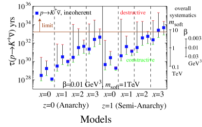
Figure 2: Plot of proton partial lifetime in years for the mode $p\rightarrow K^{+}\bar{\nu}$, shown for models with $y=-1,0,1$. Models with $z=0\ (1)$ are shown on the left (right), and within each half $x$ increases from left to right, corresponding to a decrease in $\tan\beta$. The error bars are not $1\sigma$ bars. Rather, the central point corresponds to incoherent addition of amplitudes. The upper and lower ends of the ‘error bar’ are the lifetimes computed by adding the various amplitudes destructively and constructively, respectively. The horizontal line shows the experimental lower limit of $1.6\times 10^{33}$ years. The calculation was done with $m_{\mathrm{soft}}=1$ TeV and $\beta_{p}=0.01$, but the scales on the right show the overall shift that would result from changing either $m_{\mathrm{soft}}$ or $\beta_{p}$.

The first thing to notice is that many of the models are disfavored, unless they are fine-tuned to give a highly destructive interference or the supersymmetric spectrum is carefully chosen. The models that survive best are those with a high $x$ which corresponds to a lower $\tan\beta$. In fact, of the models with $x=0$ or $x=1$, only one model has a prediction above the current experimental limit even when the amplitudes are added destructively. Recall, however, that the uncertainties in $\beta_{p}$ and $m_{\mathrm{soft}}$ are not included in the error bar, which can potentially change the prediction by the factors shown graphically to the right of Figure 2. Nevertheless, it seems clear that models with $x=0$ or $x=1$ are disfavored by current proton decay limits, barring extremely delicate accidental cancellations, as was anticipated in Dreiner:2003yr based on a rough estimate. For this reason we will focus on models with $x=2$ or $x=3$ in what follows. From Figure 2 we also see that a long proton lifetime favors a semi-anarchical MNS matrix ($z=1$) and not one determined by anarchy ($z=0$). Note that the preference for $z=1$ is also consistent with the Giudice-Masiero mechanism that naturally produces a $\mu$-term of the right size. However, this preference is only mild (within the uncertainty).

The current and upcoming experiments are expected to be able to detect charged leptons with a high efficiency. It is thus interesting to also focus on modes with charged leptons in the final state. In fact, for the proton the next modes to appear after $p\to K^{+}\bar{\nu}$ are generally $p\to\pi^{0}e^{+}$, $p\to\pi^{0}\mu^{+}$, and $p\to K^{0}\mu^{+}$. In Figure 3 we specialize to models with $x=2$ or $3$ (i. e. $\tan\beta\lesssim 10$) and show the expected lifetime from all four of the above decay modes. Here we plot the lifetime computed using incoherent addition of amplitudes, but the uncertainty due to unknown $\mathcal{O}(1)$ numbers should be kept in mind. We see that most models which survive the constraint from $p\to K^{+}\bar{\nu}$ have a lifetime for $p\to\pi^{0}\mu^{+}$ that is within two or three orders of magnitude of the experimental bound, while $p\to K^{0}\mu^{+}$ is only slightly larger, and $p\to\pi^{0}e^{+}$ can potentially be smaller. This raises the exciting possibility of two or three decay modes being detected in the coming round of experiments. Figure 3 also shows how the relative decay rates can be used to distinguish models with different phenomenology. For instance, all models with $z=0$ (anarchy) have $p\to\pi^{0}e^{+}$ as the dominant decay mode with a charged lepton in the final state, whereas its lifetime is substantially higher for the models with $z=1$. In both cases $p\to\pi^{0}\mu^{+}$ and $p\to K^{0}\mu^{+}$ are comparable.

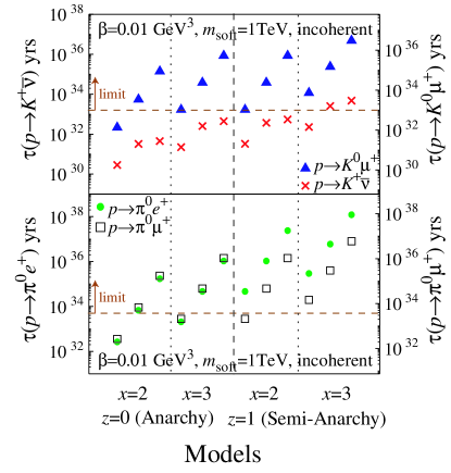
Figure 3: Comparison of proton lifetime in years for four different decay modes. The upper plot shows the computed lifetime for $p\to K^{+}\bar{\nu}$ ($\times$, left axis) and $p\to K^{0}\mu^{+}$ ($\blacktriangle$, right axis). The lower plot shows $p\to\pi^{0}e^{+}$ ($\bullet$, left axis) and $p\to\pi^{0}\mu^{+}$ ($\square$, right axis). For each plot the data for the two modes have been scaled so that the experimental limits, represented by the horizontal line, coincide, hence the different scales on the left and right axes. The lifetimes are plotted for all twelve models with $\tan\beta\lesssim 10$.

To further illustrate the differences in the pattern of decay modes from different models, we will focus on three specific models, namely Model 1 with $x=3,\ y=-1,\ z=1$, Model 2 with $x=2,\ y=1,\ z=0$, and Model 3 with $x=3,\ y=0,\ z=1$. Model 3 was specifically studied in Dreiner:2003yr . Model 2 is has a particularly nice charge assignment as shown in Table 2. In Figure 4 we show the normalized partial lifetimes for these three models in eight proton decay modes (left side) and five neutron decay modes (right side).

Various modes, if discovered, may serve as a discriminator between models. For example, among the three models shown in Figure 4, any mode involving a muon in the final state can differentiate Model 1 from Models 2 and 3. The decay mode $p\to\pi^{0}e^{+}$ can differentiate Model 2 from Model 3, etc.

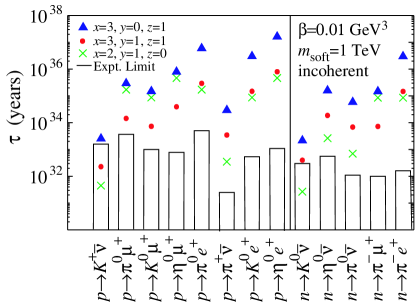
Figure 4: Plot of nucleon lifetime in years for eight proton decay modes (left side) and five neutron decay modes (right side). The different symbols represent different $U(1)_{X}$ charge assignments, namely Model 1 ($\bullet$) which has $x=3,\ y=-1,\ z=1$, Model 2 ($\times$) with $x=2,\ y=1,\ z=0$, and Model 3 ($\blacktriangle$) with $x=3,\ y=0,\ z=1$. The experimental limit for each mode is shown as a vertical column.

VI Conclusion

We have shown that the search for nucleon decay is a powerful probe of physics at the Planck scale. We focused on a a class of ambitious, string motivated, Froggatt-Nielsen models. These models explain the masses and mixings of all SM fermions while automatically enforcing $R$-parity as an accidental symmetry. In the context of these models, we have shown that operators suppressed by the Planck scale lead to nucleon decay rates that are generically right near the current experimental limits, even without Grand Unification. In fact, current bounds disfavor many of the 24 distinct models of this type.

The main unknown in this program is whether supersymmetry exists, and if so, what the mass spectrum is. Data from the LHC and a Linear Collider, along with improved lattice calculations of the matrix element, will remove much of the uncertainty (see Fig. 2) leaving us with much tighter constraints. Furthermore, discovery of several proton decay modes would serve as a good discriminator between the various model parameters. Similarly, a measurement of $\theta_{13}$ in neutrino experiments, or of $\tan\beta$ at a collider, can help narrowing down the choice of viable models. We thus conclude that upcoming experiments may truly be probing physics at the Planck scale.

Appendix A Dressing Diagrams

The superpotential operators $Q_{i}Q_{j}Q_{k}L_{l}$ and ${\,\overline{\!U}{}}_{i}{\,\overline{\!U}{}}_{j}{\,\overline{\!D}{}}_{k}{\,\overline{\!E}{}}_{l}$ are not all independent. In particular,

$$Q_{i}Q_{j}Q_{k}L_{l}\, = Q_{j}Q_{i}Q_{k}L_{l}\,$$

$$Q_{i}Q_{j}Q_{i}L_{l}\, = -\frac{1}{2}Q_{i}Q_{i}Q_{j}L_{l}\,\ \mbox{ (no sum) }$$ (25)

$${\,\overline{\!U}{}}_{i}{\,\overline{\!U}{}}_{j}{\,\overline{\!D}{}}_{k}{\,\overline{\!E}{}}_{l}\, = -{\,\overline{\!U}{}}_{j}{\,\overline{\!U}{}}_{i}{\,\overline{\!D}{}}_{k}{\,\overline{\!E}{}}_{l}\,.$$

Furthermore, contributions to nucleon decay can only come from operators with at least one first generation superfield. The list of independent operators that contribute to proton decay is shown in Table 4. Since we do not know the exact $\mathcal{O}(1)$ coefficients in front of these operators, we will simply work with an independent basis of operators and assume that their unknown coefficients are given by the $\epsilon$-suppression determined by the $X$-charges times $\mathcal{O}(1)$ numerical factors, excluding accidental cancellations.

Operator	Independent set of $(ijkl)$
$Q_{i}Q_{j}Q_{k}L_{l}$	$(112l),(113l),(221l),(331l),(123l),(132l),(231l)$
${\,\overline{\!U}{}}_{i}{\,\overline{\!U}{}}_{j}{\,\overline{\!D}{}}_{k}{\,\overline{\!E}{}}_{l}$	$(121l),(122l),(123l),(131l),(132l),(133l)$

Table 4: Independent operators relevant for nucleon decay as labeled by their generation indices.

The operators are then dressed by a gaugino or higgsino as shown in Figure 1. In general, there are many ways each diagram can be dressed. However, it has been long known that in the limit of degenerate squarks many dressing combinations cancel due to a Fierz identity Belyaev:ik ; Babu:1995cw . Here we demonstrate this cancellation explicitly using gluino dressing as an example, following the description in Goh:2003nv . Because gluinos are flavor blind, they couple to up- and down-type squarks equally and do not change flavor. Since they do not couple to leptons, there are three ways that gluinos can dress a given operator ${\,\overline{\!U}{}}_{i}{\,\overline{\!U}{}}_{j}{\,\overline{\!D}{}}_{k}{\,\overline{\!E}{}}_{l}$.

$$1: f({\,\overline{\!U}{}}_{i},{\,\overline{\!U}{}}_{j})\;({\,\overline{\!E}{}}_{l}{\,\overline{\!D}{}}_{k})({\,\overline{\!U}{}}_{i}{\,\overline{\!U}{}}_{j})$$

$$2: f({\,\overline{\!U}{}}_{i},{\,\overline{\!D}{}}_{k})\;({\,\overline{\!E}{}}_{l}{\,\overline{\!U}{}}_{j})({\,\overline{\!D}{}}_{k}{\,\overline{\!U}{}}_{i})$$ (26)

$$3: f({\,\overline{\!D}{}}_{k},{\,\overline{\!U}{}}_{j})\;({\,\overline{\!E}{}}_{l}{\,\overline{\!U}{}}_{i})({\,\overline{\!U}{}}_{j}{\,\overline{\!D}{}}_{K})$$

In these expressions the fields are Weyl spinors contracted within the parentheses. The function $f(x,y)$ comes from the loop integral and depends on the masses of the gluino and the squarks $x$ and $y$. Thus $f(x,y)$ encodes all the flavor dependence, so in the limit of degenerate squarks each factor of $f$ above is common to all three terms. The interesting fact is that the sum of those three operators vanishes by the following Fierz identity:

$$(AB)(CD)+(AD)(BC)+(AC)(DB)=0,$$ (27)

which can be easily shown by rewriting the epsilon tensors used to contract the pairs of Weyl spinors in terms of Kronecker delta functions. Thus the sum of the three operators in Eqn. (A) will vanish whenever they all have the same coefficient out front, which occurs in the degenerate squark limit. This can also be explained in words by noting that in the final four-fermion operator the three quark fields must be antisymmetric in color, antisymmetric in flavor (not generation, but flavor) and, since they are fermions, antisymmetric in spin as well to make the total operator antisymmetric under fermion exchange. But since there are three quark fields but only two spin states for each Weyl spinor, there is no way to make an operator that is completely antisymmetric in spin, hence the whole collection must vanish.

This argument holds for all the gluino dressings of $Q_{i}Q_{j}Q_{k}L_{l}$ and ${\,\overline{\!U}{}}_{i}{\,\overline{\!U}{}}_{j}{\,\overline{\!D}{}}_{k}{\,\overline{\!E}{}}_{l}$. In addition, it also holds for bino dressing of $Q_{i}Q_{j}Q_{k}L_{l}$ Goh:2003nv . The bino and neutral higgsino dressings of ${\,\overline{\!U}{}}_{i}{\,\overline{\!U}{}}_{j}{\,\overline{\!D}{}}_{k}{\,\overline{\!E}{}}_{l}$ do not lead to any operators that contribute to nucleon decay, due to the inevitable presence of 2nd or 3rd generation up-quarks. Thus the only relevant dressing of the $SU(2)$ singlet fields in ${\,\overline{\!U}{}}_{i}{\,\overline{\!U}{}}_{j}{\,\overline{\!D}{}}_{k}{\,\overline{\!E}{}}_{l}$ is by charged higgsinos. The $Q_{i}Q_{j}Q_{k}L_{l}$ operators get contributions from charged and neutral winos and higgsinos. In general, the dominant contributions are usually from wino dressing of $Q_{i}Q_{j}Q_{k}L_{l}$ , except for the ${\,\overline{\!U}{}}_{i}{\,\overline{\!U}{}}_{j}{\,\overline{\!D}{}}_{k}{\,\overline{\!E}{}}_{l}$ contribution to the $K\nu_{\tau}$ final state when $\tan\beta$ is large, as pointed out by Goto:1998qg .

Appendix B TRANSFORMING INTO THE MASS BASIS

Once the flavon acquires a VEV the coefficients $C^{ijkl}_{L,R}$ are each determined by a dimensionless $\mathcal{O}(1)$ coefficient times an $\epsilon$-suppression. In principle, some coefficients may be exactly zero due to negative overall $X$-charge, the so-called “supersymmetric zeros”, but this does not occur in the models we consider. The naive $C^{ijkl}_{L,R}$ cannot be directly plugged into Eqn. (24). First one needs to take into account two superfield-transformations, namely the canonicalization of the Kähler potential (CK), and then the transformation into the mass basis of the quarks and leptons (TM):

1. From the outset the Kähler potential need not have the canonical form (see Leurer:1992wg ; Feinberg:1959ui ; Binetruy:1996xk ; Dreiner:2003hw ; Jack:2003pb for details). For example, the Kähler potential for the quark doublets takes the form

   $$\overline{Q}_{i}~{}{H_{\!Q}}^{\!ij}~{}Q_{j}~{}=~{}\overline{\boldsymbol{\Big{[}{\boldsymbol{\mathcal{C}_{\!Q}}}\cdot Q}\Big{]}}_{i}~{}~{}\delta^{ij}~{}~{}\Big{[}\boldsymbol{{\boldsymbol{\mathcal{C}_{\!Q}}}\cdot Q}\Big{]}_{j}$$ (28)

   where $\boldsymbol{H_{\!Q}}$ is a Hermitian matrix with hierarchical entries, generated when the flavon acquires a VEV. It can be diagonalized by the matrix $\boldsymbol{\mathcal{C}_{\!Q}}$. This redefinition, i.e. the “CK”, affects the coupling constants of the superpotential, e.g.

   $$\boldsymbol{G_{\!U}}~{}\rightarrow~{}\boldsymbol{{G_{\!U}}^{\!C\!K}}=\frac{1}{\sqrt{H^{\left(H^{\mathcal{U}}\right)}~{}}}~{}{{\boldsymbol{\mathcal{C}_{\!Q}}}^{-1}}^{T}\cdot\boldsymbol{G_{\!U}}\cdot{\boldsymbol{\mathcal{C}_{\!\overline{U}}}}^{-1}.$$ (29)

2. Transforming the superfields to the mass basis, the coupling constants are then subject to the “TM”. One has

   $$\boldsymbol{{G_{\!U}}^{\!C\!K}}~{}=~{}\boldsymbol{\mathcal{U}_{U_{\!L}}}^{\!T}\cdot\mbox{{\bf{diag}}}\{m_{u},m_{c},m_{t}\}\cdot\boldsymbol{\mathcal{U}_{\overline{U_{\!R}}}},$$ (30)

   etc., the $\boldsymbol{\mathcal{U}}_{...}$ being unitary.

The other superpotential coupling constants have to be transformed correspondingly, e.g.

$$C^{ijkl}_{R}\rightarrow{C_{R}^{C\!K\!+\!T\!M}}^{~{}ijkl}=\Big{[}\big{(}\boldsymbol{\mathcal{U}_{\overline{U_{\!R}}}}\cdot\boldsymbol{\mathcal{C}_{\!\overline{U}}}\big{)}^{-1}\Big{]}^{~{}i}_{\!i^{\prime}}~{}\Big{[}\big{(}\boldsymbol{\mathcal{U}_{\overline{U_{\!R}}}}\cdot\boldsymbol{\mathcal{C}_{\!\overline{U}}}\big{)}^{-1}\Big{]}^{~{}j}_{\!j^{\prime}}~{}\Big{[}\big{(}\boldsymbol{\mathcal{U}_{\overline{D_{\!R}}}}\cdot\boldsymbol{\mathcal{C}_{\!\overline{D}}}\big{)}^{-1}\Big{]}^{~{}k}_{\!k^{\prime}}~{}\Big{[}\big{(}\boldsymbol{\mathcal{U}_{\overline{E_{\!R}}}}\cdot\boldsymbol{\mathcal{C}_{\!\overline{E}}}\big{)}^{-1}\Big{]}^{~{}l}_{\!l^{\prime}}~{}C^{i^{\prime}j^{\prime}k^{\prime}l^{\prime}}_{R}.$$ (31)

As we lack knowledge of the $\mathcal{O}(1)$ coefficients, this can only be done approximately, supposing no accidental cancellations. One can show Binetruy:1996xk that

$$\Big{[}\boldsymbol{{{\mathcal{C}_{\!Q}}}}^{-1}\Big{]}_{\!ij}~{}\sim~{}\epsilon^{|X_{Q^{i}}-X_{Q^{j}}|},~{}~{}\mbox{etc.},$$ (32)

from which it follows that the CK fills up supersymmetric zeros but does not change the $\epsilon$-suppression of any other nonzero entries. Using Table 1 this gives

$$\boldsymbol{{{\mathcal{C}_{\!Q}}}}^{-1} \sim \left(\begin{array}[]{ccc}1&\epsilon^{|1+y|}&\epsilon^{|3+y|}\\ \epsilon^{|1+y|}&1&\epsilon^{2}\\ \epsilon^{|3+y|}&\epsilon^{2}&1\end{array}\right),$$ (36)

$$\boldsymbol{{{\mathcal{C}_{\!L}}}}^{-1} \sim \left(\begin{array}[]{ccc}1&\epsilon^{z}&\epsilon^{z}\\ \epsilon^{z}&1&1\\ \epsilon^{z}&1&1\end{array}\right),$$ (40)

$$\boldsymbol{{{\mathcal{C}_{\!\overline{D}}}}}^{-1} \sim \left(\begin{array}[]{ccc}1&\epsilon^{|1-y|}&\epsilon^{|1-y|}\\ \epsilon^{|1-y|}&1&1\\ \epsilon^{|1-y|}&1&1\end{array}\right),$$ (44)

$$\boldsymbol{{{\mathcal{C}_{\!\overline{U}}}}}^{-1} \sim \left(\begin{array}[]{ccc}1&\epsilon^{|3-y|}&\epsilon^{|5-y|}\\ \epsilon^{|3-y|}&1&\epsilon^{2}\\ \epsilon^{|5-y|}&\epsilon^{2}&1\end{array}\right),$$ (48)

$$\boldsymbol{{{\mathcal{C}_{\!\overline{E}}}}}^{-1} \sim \left(\begin{array}[]{ccc}1&\epsilon^{2}&\epsilon^{4}\\ \epsilon^{2}&1&\epsilon^{2}\\ \epsilon^{4}&\epsilon^{2}&1\end{array}\right).$$ (52)

The $\boldsymbol{\mathcal{U}}_{...}$ are given in Table 5, having used the expressions in Hall:1993ni .

$\boldsymbol{\mathcal{U}_{U_{\!L}}}^{*},~{}\boldsymbol{\mathcal{U}_{D_{\!L}}}^{*}$	$\boldsymbol{\mathcal{U}_{\overline{U_{\!R}}}}^{\dagger}$	$\boldsymbol{\mathcal{U}_{\overline{D_{\!R}}}}^{\dagger}$	$\boldsymbol{\mathcal{U}_{E_{\!L}}}^{*},~{}\widetilde{\boldsymbol{\mathcal{U}_{N_{\!L}}}}^{*}~{}$	$\boldsymbol{\mathcal{U}_{\overline{E_{\!R}}}}^{\dagger}$
$~{}\left(\begin{array}[]{ccc}1&\epsilon^{1+y}&\epsilon^{3+y}\\ \epsilon^{1+y}&1&\epsilon^{2}\\ \epsilon^{3+y}&\epsilon^{2}&1\end{array}\right)^{~{}\phantom{\Big{|}}}_{~{}\phantom{\Big{|}}}$	$~{}\left(\begin{array}[]{ccc}1&\epsilon^{3-y}&\epsilon^{5-y}\\ \epsilon^{3-y}&1&\epsilon^{2}\\ \epsilon^{5-y}&\epsilon^{2}&1\end{array}\right)~{}$	$~{}\left(\begin{array}[]{ccc}1&\epsilon^{1-y}&\epsilon^{1-y}\\ \epsilon^{1-y}&1&1\\ \epsilon^{1-y}&1&1\end{array}\right)~{}$	$~{}\left(\begin{array}[]{ccc}1&\epsilon^{z}&\epsilon^{z}\\ \epsilon^{z}&1&1\\ \epsilon^{z}&1&1\end{array}\right)^{~{}\phantom{\Big{|}}}_{~{}\phantom{\Big{|}}}$	$~{}\left(\begin{array}[]{ccc}1&\epsilon^{2}&\epsilon^{4}\\ \epsilon^{2}&1&\epsilon^{2}\\ \epsilon^{4}&\epsilon^{2}&1\end{array}\right)^{~{}\phantom{\Big{|}}}_{~{}\phantom{\Big{|}}}$

Table 5: The matrices needed to perform the TM. For the quarks they are valid for any $X$-charge assignment which leads to the five pairs of quark mass matrices displayed in Dreiner:2003yr . The ones for the leptons ($y$-independent) are only valid for the $X$-charge assignment used in this article. $\widetilde{\boldsymbol{\mathcal{U}_{N_{\!L}}}}^{*}$ is the almost unitary matrix which Schur-diagonalizes the symmetric mass matrix of the light neutrinos. Note that these approximate TM matrices reproduce the CKM matrix and the MNS matrix, as they should.

Since the $C_{R,L}^{ijkl}$ we consider do not have any supersymmetric zeros, their $\epsilon$-dependence is not changed by the CK. As for TM, comparing Table 5 with the $\boldsymbol{\mathcal{C}_{...}}$ given above, one finds e.g. $~{}\boldsymbol{\mathcal{U}_{U_{\!L}}}^{*}\sim\boldsymbol{\mathcal{C}_{\!Q}}~{}$ and $~{}\boldsymbol{\mathcal{U}_{\overline{U_{\!R}}}}^{\dagger}\sim\boldsymbol{\mathcal{C}_{{\!\overline{U}}}}$. Since $\boldsymbol{\mathcal{C}_{\!Q}}^{2}\sim\boldsymbol{\mathcal{C}_{\!Q}}$ (and likewise for the others), we find that the $C^{ijkl}_{L,R}$ are not changed substantially when going into the mass basis either. Thus the naively calculated $\epsilon$-suppression for $C^{ijkl}_{L,R}$ remains the same after changing to the mass basis.

References

- (1) A. D. Sakharov, Pisma Zh. Eksp. Teor. Fiz. 5, 32 (1967) [JETP Lett. 5, 24 (1967 SOPUA,34,392-393.1991 UFNAA,161,61-64.1991)].
-
(2)
E. Kearns, Talk at Snowmass 2001,
http://hep.bu.edu/~kearns/pub/kearns-pdk-snowmass.pdf. - (3) H. Murayama and A. Pierce, Phys. Rev. D 65, 055009 (2002) [arXiv:hep-ph/0108104].
- (4) H. Murayama and D. B. Kaplan, Phys. Lett. B 336, 221 (1994) [arXiv:hep-ph/9406423].
- (5) C. D. Froggatt and H. B. Nielsen, Nucl. Phys. B 147, 277 (1979).
- (6) H. K. Dreiner and M. Thormeier, Phys. Rev. D 69, 053002 (2004) [arXiv:hep-ph/0305270].
- (7) M. Kakizaki and M. Yamaguchi, JHEP 0206, 032 (2002) [arXiv:hep-ph/0203192].
- (8) N. Arkani-Hamed and M. Schmaltz, Phys. Rev. D 61, 033005 (2000) [arXiv:hep-ph/9903417];
- (9) M. Kakizaki and M. Yamaguchi, arXiv:hep-ph/0110266.
- (10) H. K. Dreiner, H. Murayama and M. Thormeier, arXiv:hep-ph/0312012.
- (11) M. B. Green and J. H. Schwarz, Phys. Lett. B 149, 117 (1984).
- (12) M. Dine, N. Seiberg, X. G. Wen and E. Witten, Nucl. Phys. B 289, 319 (1987).
- (13) M. Dine, N. Seiberg, X. G. Wen and E. Witten, Nucl. Phys. B 278, 769 (1986).
- (14) J. J. Atick, L. J. Dixon and A. Sen, Nucl. Phys. B 292, 109 (1987).
- (15) M. Dine, I. Ichinose and N. Seiberg, Nucl. Phys. B 293, 253 (1987).
- (16) J. R. Espinosa and A. Ibarra, arXiv:hep-ph/0405095.
- (17) S. F. King, I. N. R. Peddie, G. G. Ross, L. Velasco-Sevilla and O. Vives, arXiv:hep-ph/0407012.
- (18) L. J. Hall, H. Murayama and N. Weiner, Phys. Rev. Lett. 84, 2572 (2000) [arXiv:hep-ph/9911341],
- (19) N. Haba and H. Murayama, Phys. Rev. D 63, 053010 (2001) [arXiv:hep-ph/0009174].
- (20) J. Sato and T. Yanagida, Phys. Lett. B 430, 127 (1998) [arXiv:hep-ph/9710516].
- (21) G. F. Giudice and A. Masiero, Phys. Lett. B 206, 480 (1988).
- (22) J. E. Kim and H. P. Nilles, Mod. Phys. Lett. A 9, 3575 (1994) [arXiv:hep-ph/9406296].
- (23) T. Goto and T. Nihei, Phys. Rev. D 59, 115009 (1999) [arXiv:hep-ph/9808255].
- (24) M. Claudson, M. B. Wise and L. J. Hall, Nucl. Phys. B 195, 297 (1982).
- (25) A. J. Buras, J. R. Ellis, M. K. Gaillard and D. V. Nanopoulos, Nucl. Phys. B 135, 66 (1978).
- (26) Y. Kuramashi [JLQCD Collaboration], arXiv:hep-ph/0103264.
- (27) Y. Aoki [RBC Collaboration], Nucl. Phys. Proc. Suppl. 119, 380 (2003) [arXiv:hep-lat/0210008].
- (28) K. Hagiwara et al. [Particle Data Group Collaboration], Phys. Rev. D 66, 010001 (2002).
- (29) K. S. Babu and S. M. Barr, Phys. Lett. B 381, 137 (1996) [arXiv:hep-ph/9506261].
- (30) V. M. Belyaev and M. I. Vysotsky, Phys. Lett. B 127, 215 (1983).
- (31) H. S. Goh, R. N. Mohapatra, S. Nasri and S. P. Ng, arXiv:hep-ph/0311330.
- (32) M. Leurer, Y. Nir and N. Seiberg, Nucl. Phys. B 398, 319 (1993) [arXiv:hep-ph/9212278].
- (33) G. Feinberg, P. Kabir and S. Weinberg, Phys. Rev. Lett. 3, 527 (1959).
- (34) P. Binétruy, S. Lavignac and P. Ramond, Nucl. Phys. B 477, 353 (1996) [arXiv:hep-ph/9601243].
- (35) I. Jack, D. R. T. Jones and R. Wild, Phys. Lett. B 580, 72 (2004) [arXiv:hep-ph/0309165].
- (36) L. J. Hall and A. Rasin, Phys. Lett. B 315, 164 (1993) [arXiv:hep-ph/9303303].