IFT-2003-30

CJK-Improved 5 Flavour LO Parton Distributions in the Real Photon

Abstract

Radiatively generated, LO quark ($u,d,s,c,b$) and gluon densities in the real, unpolarized photon, improved in respect to our previous paper [1], are presented. We perform three global fits to the $F_{2}^{\gamma}$ data, using the LO DGLAP evolution equation. We improve the treatment of the strong coupling running and used lower values of $\Lambda_{QCD}$, as we have found that the too high values adopted in the previous work caused the high $\chi^{2}$ of the fits. In addition to the modified FFNS_CJKL model, referred to as FFNS_CJK1 we analyse a FFNS_CJK2 model in which we take into account the resolved-photon heavy-quark contribution. New CJK model with an improved high-$x$ behaviour of the $F_{2}^{\gamma}(x,Q^{2})$ is proposed. Finally, in the case of the CJK model we abandon the valence sum rule imposed on the VMD input densities. New fits give $\chi^{2}$ per degree of freedom about 0.25 better than the old results. All features of the CJKL model, such as the realistic heavy-quark distributions, good description of the LEP data on the $Q^{2}$ dependence of the $F_{2}^{\gamma}$ and on $F_{2,c}^{\gamma}$ are preserved. Moreover we present results of an analysis of the uncertainties of the CJK parton distributions due to the experimental errors. It is based on the Hessian method used for the proton and very recently applied for the photon by one of us. Parton and structure function parametrizations of the best fits in both FFNS_CJK and CJK approaches are made accessible. For the CJK model we provide also sets of test parametrizations which allow for calculation of uncertainties of any physical value depending on the real photon parton densities.

1 Introduction

In this paper we continue our recent analysis of the LO unpolarized real photon parton distributions, [1], improving and broadening our research. The main topic of our previous work was the description, within the DGLAP evolution framework, of the heavy, charm- and bottom-, quark contributions to the photon structure-function, $F_{2}^{\gamma}(x,Q^{2})$. We analysed and compared two approaches In the first analysed model, referred to as FFNS_CJKL, we adopted a widely used massive quark approach in which heavy quark, $h$, contributes to the photon structure only through the so-called Bethe-Heitler, $\gamma^{*}\gamma\to h\bar{h}$ process. In such models the heavy-quark masses are kept to their physical values. In the second, CJKL model, we used the ACOT$(\chi)$ [4] scheme, where heavy-quark densities appear. It was the very first application of this scheme to the photon structure. We performed two global fits to the set of updated $F_{2}^{\gamma}(x,Q^{2})$ data collected in various $e^{+}e^{-}$ experiments. We based both models on the idea of radiatively generated parton distributions introduced by the GRV group (see [5] for the photonic case).

In this work the main assumptions of the previous analysis are left unchanged, although some details are improved, and we analyse an additional model. First of all, we improve the description of the running of the strong coupling constant, $\alpha_{s}$, and use $\Lambda_{QCD}^{(4)}$ value substantially smaller than the one used previously. The $\Lambda_{QCD}$ values applied in the former analysis were obtained with the assumption that the LO and NLO $\Lambda_{QCD}$ values for four active flavours are equal, as in the GRV analysis. They appeared to be too high and were one of the causes for the high $\chi^{2}$ of the fits.

The old FFNS_CJKL model is now being denoted as FFNS_CJK1. We compare it with the more realistic model FFNS_CJK2, in which we include the so-called “resolved-photon” contribution to $F_{2}^{\gamma}(x,Q^{2})$ given by the $\gamma^{*}G^{\gamma}\to h\bar{h}$ process [6]. As we stated already in [1], the CJKL type model needs correction which could resolve the problem of the high-$x$ behaviour of $F_{2}^{\gamma}(x,Q^{2})$, predicted by this model. Therefore, we analyse a new CJK model in which this problem is avoided. The CJK model is further slightly improved by changing the lower limit of the integration, in the heavy-quark subtraction terms, from the square of the mass of the heavy quark, $m_{h}^{2}$, to the starting scale of the DGLAP evolution, $Q_{0}^{2}$. This also leads to better fits. Finally in the case of the CJK model we abandon the valence-number sum rule imposed by hand on the VMD input densities but keep the corresponding energy-momentum constraint.

Finally, in all new fits we use limited set of data, excluding the TPC2$\gamma$ data which are considered to be inconsistent with other experimental results. This is an additional reason, beyond improvements mentioned above, why our new predictions for model FFNS_CJK1 are not identical with results obtained in [1] from full set of data.

We also proceed in the direction not addressed before. We analyse uncertainties of the parton distributions due to the experimental errors of $F_{2}^{\gamma}(x,Q^{2})$ data. This part of the work has been motivated by the recent analysis performed for the proton structure by the CTEQ Collaboration, [7, 8, 9] and the MRST group, [10]. We use the Hessian method, formulated in recent papers, to obtain sets of test parton densities allowing along with the parton distributions of the best fit to calculate the best estimate and uncertainty of any observable depending on the photon structure. Full discussion has been given in [3], see also [2].

This paper is divided into four parts. Section 2 recalls the previous FFNS_CJKL and CJKL models of the real photon structure. In section 3 we explain in detail all the changes currently introduced to the models. Next, in section 4, we present results of the new fits to the experimental $F_{2}^{\gamma}(x,Q^{2})$ data along with the calculated uncertainties of the CJK parton distributions. The parton distributions which are a result of our analysis have been parametrized on the grid. In section 5 we give a short summary and information where to find the corresponding FORTAN programs.

2 FFNS_CJKL and CJKL models - short recollection

The two approaches leading to the FFNS_CJKL and CJKL models, and considered also in this analysis, have been described in detail in our previous paper [1]. The difference between them lies in the approach to the calculation of the heavy, charm- and beauty-, quark contributions to the photon structure function $F_{2}^{\gamma}(x,Q^{2})$. First, FFNS_CJKL model bases on a widely adopted Fixed Flavour-Number Scheme in which there are no heavy quarks (denoted below by $h$) as partons in the photon. Their contributions to $F_{2}^{\gamma}(x,Q^{2})$ are given by the ’direct’ (Bethe-Heitler) $\gamma^{*}\gamma\to h\bar{h}$ process. In addition one can also include the so-called ’resolved’-photon contribution: $\gamma^{*}G^{\gamma}\to h\bar{h}$. We denote these terms as $F_{2,h}^{\gamma}(x,Q^{2})|_{dir}$ and $F_{2,h}^{\gamma}(x,Q^{2})|_{res}$, respectively. In this paper we consider two FFNS models: in the first one, FFNS_CJK1, we neglect the resolved-photon contribution, while in the second one, FFNS_CJK2, both mentioned contributions to $F_{2}^{\gamma}(x,Q^{2})$ are included. The photon structure function is then computed as

$$F_{2}^{\gamma}(x,Q^{2})=\sum_{i=1}^{3}xe_{i}^{2}(q_{i}^{\gamma}+\bar{q}_{i}^{\gamma})(x,Q^{2})+\sum_{h(=c,b)}\left[F_{2,h}^{\gamma}(x,Q^{2})|_{dir}+F_{2,h}^{\gamma}(x,Q^{2})|_{res}\right],$$ (1)

with $q^{\gamma}_{i}(x,Q^{2})$ ($\bar{q}^{\gamma}_{i}(x,Q^{2})$) being the light $u,d,s$ quark (anti-quark) densities, governed by the LO Dokshitzer-Gribov-Lipatov-Altarelli-Parisi (DGLAP) evolution equations, [11].

The CJKL model adopts the new ACOT($\chi$) scheme, [4], which is a recent realization of the General Variable-Flavour Number Scheme (GVFNS). In this scheme one combines the Zero-mass Variable-Flavour Number Scheme (ZVFNS), where the heavy quarks are considered as massless partons of the photon, with the FFNS just discussed above. In this model, in addition to the terms shown in Eq. (1), one must include the contributions due to the heavy-quark densities which now appear also in the DGLAP evolution equations. A double counting of the heavy-quark contributions to $F_{2}^{\gamma}(x,Q^{2})$ must be corrected with the introduction of subtraction terms for both, the direct- and resolved-photon, contributions. Further, following the ACOT($\chi$) scheme, we introduce the $\chi_{h}=x(1+4m_{h}^{2}/Q^{2})$ variables giving the proper vanishing of the heavy-quark densities at the kinematic thresholds for their production in DIS: $W^{2}=Q^{2}(1-x)/x>4m_{h}^{2}$, where $W$ is the $\gamma^{*}\gamma$ centre of mass energy. Adequate substitution of $x$ with $\chi_{h}$ in $q_{h}$ and the subtraction terms forces their correct threshold behaviour, as $\chi_{h}\to 1$ when $W\to 2m_{h}$. This is achieved for all terms except for the direct subtraction term $F_{2,h}^{\gamma}(x,Q^{2})|_{dir,sub}$ for which there is a need of an additional condition, $F_{2,h}^{\gamma}(x,Q^{2})|_{dir,sub}=0$ for $\chi_{h}>1$. The full formula for the photon structure function in the CJKL model is

$$F_{2}^{\gamma}(x,Q^{2}) = x\sum_{i=1}^{3}e_{i}^{2}(q_{i}^{\gamma}+\bar{q}_{i}^{\gamma})(x,Q^{2})+x\sum_{h(=c,b)}e_{h}^{2}(q_{h}^{\gamma}+\bar{q}_{h}^{\gamma})(\chi_{h},Q^{2})$$

$$+\sum_{h(=c,b)}\left[F_{2,h}^{\gamma}(x,Q^{2})|_{dir}+F_{2,h}^{\gamma}(x,Q^{2})|_{res}\right]$$

$$-\sum_{h(=c,b)}\left[F^{\gamma}_{2,h}|_{dir,sub}(\chi_{h},Q^{2})+F^{\gamma}_{2,h}|_{res,sub}(\chi_{h},Q^{2})\right].$$

with positivity constraint for each heavy-quark contribution , $F_{2,h}^{\gamma}(x,Q^{2})>0$. Explicit expressions for the terms appearing in Eqs. (1) and (2) can be found in [1].

We use the DGLAP equations summing the QCD corrections in form of leading logarithms of $Q^{2}$. Their solution for quark densities can be divided into the so-called point-like (pl) part, equal to a special solution of the full inhomogeneous equation and the hadron-like (had) part, arising as a general solution of the homogeneous equation. Their sum gives the partonic density in the photon. It is most useful to write the result in the Mellin-moments space with the $n$th moment defined as

$$f^{n}(Q^{2})=\int_{0}^{1}x^{n-1}f(x,Q^{2})dx,$$ (3)

where $f(x,Q^{2})$ can be the parton (quark and gluon) densities, $q^{\gamma}(x,Q^{2})$, or the splitting functions in the DGLAP evolution equations $P(x,Q^{2})$ and $k(x,Q^{2})$ defined in [1]. Then one obtains

$$q^{\gamma,n}(Q^{2})=q_{\mathrm{had}}^{\gamma,n}(Q^{2})+q_{\mathrm{pl}}^{\gamma,n}(Q^{2}),$$ (4)

where

$$q_{\mathrm{pl}}^{\gamma,n}(Q^{2}) = \frac{4\pi}{\alpha_{s}(Q^{2})}\frac{1}{1-2P^{n}/\beta_{0}}\frac{\alpha}{2\pi\beta_{0}}\left[1-L^{1-2P^{n}/\beta_{0}}\right]k^{n},$$

(5)

$$q_{\mathrm{had}}^{\gamma,n}(Q^{2}) = L^{-2P^{n}/\beta_{0}}q^{\gamma,n}(Q_{0}^{2}).$$

Here $L=\frac{\alpha_{s}(Q^{2})}{\alpha_{s}(Q_{0}^{2})}$, where $Q_{0}^{2}$ is the scale at which the evolution starts (we call it the input scale).

For all models we choose to start the DGLAP evolution at small value of the $Q^{2}$ scale, $Q_{0}^{2}=0.25$ GeV², following GRV [5] hence our parton densities are radiatively generated. As it is seen above the point-like contributions are calculable without further assumptions, while the hadronic parts need input distributions. For this purpose we utilize the Vector Meson Dominance (VMD) model [12], where

$$f_{had}^{\gamma}(x,Q_{0}^{2})=\sum_{V}\frac{4\pi\alpha}{\hat{f}^{2}_{V}}f^{V}(x,Q_{0}^{2}),$$ (6)

with the sum running over all light vector mesons (V) into which the photon can fluctuate. The parameters $\hat{f}^{2}_{V}$ can be extracted from the experimental data on the $\Gamma(V\to e^{+}e^{-})$ width. In this analysis we use explicitely the $\rho^{0}$-meson densities while the contributions from other mesons are accounted for via a parameter $\kappa$, that is left as a free parameter. Thus, we take the parton densities in the photon equal to

$$f_{had}^{\gamma}(x,Q_{0}^{2})=\kappa\frac{4\pi\alpha}{\hat{f}^{2}_{\rho}}f^{\rho}(x,Q_{0}^{2}).$$ (7)

We take the input densities of the $\rho^{0}$ meson at $Q_{0}^{2}=0.25$ GeV² in the form of valence-like distributions both for the (light) quark ($v^{\rho}$) and gluon ($G^{\rho}$) densities. All sea-quark distributions (denoted as $\zeta^{\rho}$), including $s$-quarks, are neglected at the input scale.

The valence-quark and gluon densities satisfy the energy-momentum sum rule for $\rho^{0}$:

$$\int_{0}^{1}x(2v^{\rho}(x,Q_{0}^{2})+G^{\rho}(x,Q_{0}^{2}))dx=1,$$ (8)

and the sum rule related to the number of valence quarks, $n_{v}$

$$n_{v}=\int_{0}^{1}2v^{\rho}(x,Q_{0}^{2})=2.$$ (9)

Both of them we imposed as constraints on the parameters of the models in our previous analysis [1].

The input quark and gluon densities are taken in the form (with $\alpha>0$)

$$xv^{\rho}(x,Q_{0}^{2}) = N_{v}x^{\alpha}(1-x)^{\beta},$$

$$xG^{\rho}(x,Q_{0}^{2}) = \tilde{N}_{g}xv^{\rho}(x,Q_{0}^{2})=N_{g}x^{\alpha}(1-x)^{\beta},$$ (10)

$$x\zeta^{\rho}(x,Q_{0}^{2}) = 0,$$

where $N_{g}=\tilde{N}_{g}N_{v}$. The imposed constraint given by Eq. (8) allows to express the normalization factor $N_{g}$ as a function of $\alpha,\beta$ and $N_{v}$. Moreover, when constraint (9) is imposed the $N_{v}$ parameter can be further expressed in terms of $\alpha$ and $\beta$. In the former case there are three and in the letter case four free parameters left as a subject to the global fit to the $F_{2}^{\gamma}(x,Q^{2})$ data.

3 New analysis

We have performed new fits with a slightly changed data set as compared to the previous work. Moreover, in our new analysis we improved the treatment of the running of $\alpha_{s}$, by differentiating the number of active quarks in the running of $\alpha_{s}$ and in the evolution equations, and by using lower values of $\Lambda_{QCD}$. We first describe new aspects of our analysis which are common to all considered models. Aspects relevant only for the CJK model are discussed next.

3.1 Data Set

New fits were performed using all existing $F_{2}^{\gamma}(x,Q^{2})$ data, [14, 15, 16, 17, 18, 19, 20, 21, 22, 23, 24], apart from the old TPC2$\gamma$, [25]. In our former global analysis [1] we used 208 $F_{2}^{\gamma}(x,Q^{2})$ experimental points. Now we decided to exclude the TPC2$\gamma$ data from the set because it has been pointed out (see for instance [26]) that these data are not in agreement with other measurements. A detailed study of the influence of various $F_{2}^{\gamma}$ data sets on the fits is performed by one of us in [3]. After the exclusion of the TPC2$\gamma$ data we are left with 182 $F_{2}^{\gamma}(x,Q^{2})$ experimental points. We include all these data in the $\chi^{2}$ fit without any weights. A list of all experimental points used can be found on the web-page [27].

The exclusion of the TPC2$\gamma$ points affects the $\chi^{2}/_{\rm DOF}$ of the fits but has very small influence on the shape of the resulting parton distributions.

3.2 $\alpha_{s}$ running and values of $\Lambda^{(N_{q})}$

The running of the strong coupling constant at lowest order is given by the well-known formula:

$$\alpha_{s}^{(N_{q})}(Q^{2})=\frac{4\pi}{\beta_{0}\ln Q^{2}/(\Lambda^{(N_{q})})^{2}}\quad\mathrm{with}\quad\beta_{0}=11-\frac{2}{3}N_{q},$$ (11)

where $N_{q}$ is the number of quarks entering in the $\alpha_{s}$ evaluation. This number increases by one unit whenever $Q^{2}$ reaches a heavy-quark threshold, i.e. when $Q^{2}=m_{h}^{2}$, where the condition $\alpha_{s}^{(N_{q})}(m_{h}^{2})=\alpha_{s}^{(N_{q}+1)}(m_{h}^{2})$ is imposed in order to ensure the continuity of the strong coupling constant.

In our previous analysis $N_{f}$ was identified with the number of active quarks in the photon: $N_{f}=3$ and $5$ in the FFNS_CJKL and CJKL models, respectively. Since we now distinguish between both numbers of quarks we have to use slightly more complicated formulea for the evolution of the parton densities, as now the above equations depend also on $N_{q}$ through their dependence on $\alpha_{s}(Q^{2})$ and $\beta_{0}$. Because of the implicit introduction of the heavy-quark thresholds into the $\alpha_{s}$ running we must proceed in three steps to perform the DGLAP evolution. In the first step, describing the evolution from the input scale $Q_{0}$ to the charm-quark mass $m_{c}$, the hadronic input $q_{\mathrm{had}}^{\gamma}(x,Q_{0}^{2})$ is taken from the VMD model. In the second step we evolve the parton distributions from $m_{c}$ to the beauty-quark mass, $m_{b}$ and in the third one we start at $m_{b}$. In the second and third steps a new hadronic input at $Q^{2}=m_{h}^{2}$ is given by the sum of the already evolved hadronic and point-like contributions and the point-like distribution at this scale becomes zero again.

In the previous work we assumed (following the GRV group approach [5]) that the LO and NLO $\Lambda_{QCD}$ values for four active flavours are equal. We adopted $\Lambda_{QCD}^{(4)}=280$ MeV, value given in the Particle Data Group (PDG) report [13]. We now abandon this assumption and take $\Lambda_{QCD}^{(4)}=115$ MeV, which is obtained from the world average value $\alpha_{s}(M_{Z})=0.117$, with $M_{Z}=91.188$ GeV, using the LO expression for $\alpha_{s}$ evolution, Eq. (11). As a consistency check we performed fits keeping $\Lambda_{QCD}^{(4)}$ as a free parameter and obtained results close to $115$ MeV. Since it is not our aim in this paper to extract a value of $\alpha_{s}$ from a fit to $F_{2}^{\gamma}$ data, we prefer to fix $\Lambda_{QCD}^{(4)}=115$ MeV rather than add a new free parameter in our fits. Imposing the continuity condition for the strong coupling constant and $m_{c}=1.3$ GeV and $m_{b}=4.3$ GeV, we obtain $\Lambda_{QCD}^{(3)}=138$ MeV and $\Lambda_{QCD}^{(5)}=84$ MeV.

3.3 VMD input

Like in our previous work the input evolution scale has been chosen to be small, $Q_{0}^{2}=0.25$ GeV² for both types of models and we apply the same form of the VMD model input, given by Eqs. (10) and Eq. (7).

Finally, we try to relax the constraint on number of the valence quarks, $n_{v}$, in the $\rho$ meson. This leads to 4-parameter fits. That, as will be quantitatively shown in next sections, is possible only in the case of the CJK model. Therefore in each of the new FFNS_CJK models we have 3 free parameters.

3.4 Modified subtraction terms in the CJK model

In [1] we derived the subtraction term for a direct contribution, $F_{2,h}^{\gamma}|_{dir,sub}$, from the integration of a part of the DGLAP evolution equations, namely:

$$\frac{dq_{h}^{\gamma}(x,Q^{2})}{d\ln Q^{2}}=\frac{\alpha}{2\pi}e_{h}^{2}k(x),$$ (12)

where $k(x)$ is the lowest order photon-quark splitting function (see Eq. (7) in [1]). The question here is: What should the limits of the integration be? The upper limit is obviously the $Q^{2}$ scale at which the subtraction term is calculated. For the lower limit we took previously the standard for the Bethe-Heitler process scale: $Q^{2}_{low}=m_{h}^{2}$. However, the threshold condition is $W^{2}\leq 4m_{h}^{2}$. This means that even for $Q^{2}<m_{h}^{2}$ the heavy-quark contributions do not vanish as long as the condition $x<Q^{2}/(Q^{2}+4m_{h}^{2})$ is fulfilled. Hence, in this paper we take $Q^{2}_{low}=Q^{2}_{0}$ and the direct subtraction term is given by:

$$F_{2,h}^{\gamma}|_{dir,sub}(x,Q^{2})=x\ln\frac{Q^{2}}{Q_{0}^{2}}3e_{h}^{4}\frac{\alpha}{\pi}(x^{2}+(1-x)^{2}).$$ (13)

The same discussion applies to the subtraction term for the resolved-photon contribution. So we now use

$$F_{2,h}^{\gamma}|_{res,sub}=x\ln\frac{Q^{2}}{Q_{0}^{2}}e_{h}^{2}\frac{\alpha_{s}(Q^{2})}{\pi}\int_{x}^{1}\frac{dy}{y}P_{qG}(\frac{x}{y})G^{\gamma}(y,Q^{2}).$$ (14)

instead of Eq. (19) in [1]. We found that the quality of the fit improves with this choice of the $Q^{2}_{low}$.

As we noticed in Section 2 the $x\to\chi_{h}$ substitution leads to the proper threshold behaviour of all the heavy-quark contributions to the $F_{2}^{\gamma}(x,Q^{2})$, except for the subtraction term for direct contribution. It is already seen in Eq. (13) that this term does not vanish for $\chi_{h}\to 1$ and therefore by subtracting it the resulting heavy-quark contribution to $F_{2}^{\gamma}$ may become negative in some regions of the $x$ and $Q^{2}$ plane. An extra constraint to avoid this unphysical situation is, thus, needed. In Ref. [1] we imposed the simple condition (positivity constraint) that the heavy-quark contribution to $F_{2}^{\gamma}(x,Q^{2})$ has to be positive. Unfortunately, this constraint was not strong enough and for some small windows at small and large $x$ still the unphysical situation $F_{2,h}^{\gamma}(x,Q^{2})<F_{2,h}^{\gamma}(x,Q^{2})|_{dir}+F_{2,h}^{\gamma}(x,Q^{2})|_{res}$ was found [28]. Therefore, in this analysis we apply a positivity condition in the following form:

$$F_{2,h}^{\gamma}(x,Q^{2})\geq F_{2,h}^{\gamma}(x,Q^{2})|_{dir}+F_{2,h}^{\gamma}(x,Q^{2})|_{res}.$$ (15)

4 Results of the new $F_{2}^{\gamma}$ global fits

In this analysis we determine the parameters of the models, related to the initial quark and gluon densities at the scale $Q^{2}_{0}=0.25\;GeV^{2}$, by means of the global fits to the experimental data on $F_{2}^{\gamma}(x,Q^{2})$. We use 182 $F_{2}^{\gamma}(x,Q^{2})$ experimental points, [14, 15, 16, 17, 18, 19, 20, 21, 22, 23, 24], with equal weights. Still, it has been shown in [3] that when we remove the CELLO [14] and DELPHI 2001 [20] data sets the quality of the fit improves substantially but the parton distributions lie well within the CJK uncertainties. However, we think that there is no strong argument to discard these data sets. So, we have chosen to keep them with the same weight as the other sets. Fits are based on the least-squares principle (minimum of $\chi^{2}$) and were done using Minuit [29]. Systematic and statistical errors on data points were added in quadrature.

In the CJK model we have four free parameters: $\alpha,\beta,N_{v},\kappa$, Eqs. (10) and Eq. (7). On the other hand, the two FFNS models differ only in the inclusion or not of the resolved-photon contribution to $F_{2}^{\gamma}(x,Q^{2})$(only the FFNS_CJK2 model takes it into account through the $\gamma^{*}G^{\gamma}\to h\bar{h}$ process). For both FFNS models we impose the number of valence quarks constraint (9) that allows to express $N_{v}$ in terms of $\alpha$ and $\beta$ reducing the number of free parameters to three.

The parameters of our new fits are presented in Table 1. The second and third columns show the quality of the fits, i.e. the total $\chi^{2}$ for 182 points and the $\chi^{2}$ per degree of freedom. The fitted values for parameters $\alpha$, $\beta$, $\kappa$ and $N_{v}$ are presented in the middle of the table with the errors obtained from Minos with the standard requirement of $\Delta\chi^{2}=1$. In the last column the value obtained from the constraint (8) for $\tilde{N}_{g}$ from other parameters is given.

In the case of the FFNS_CJK models the test fits with the abandoned constraint (9) gives $n_{v}\approx 0.5$ and $\approx 1.4$ in the FFNS_CJK1 and FFNS_CJK2 models, respectively. We think that it is too far away from the expected value $n_{v}=2$ . This is the reason for keeping the constraint (9) for both FFNS_CJK models. In this case the $N_{v}$ parameter is calculated from the constraint (9) and therefore we do not state its error.

model		$\chi^{2}$ (182 pts)	$\chi^{2}/_{\rm DOF}$		$\kappa$	$\alpha$	$\beta$	$N_{v}$		$\tilde{N}_{g}$
FFNSCJK1		314.0	1.754		$2.267^{+0.063}_{-0.072}$	$0.265^{+0.038}_{-0.032}$	$0.792^{+0.189}_{-0.149}$	0.358		5.02
FFNSCJK2		279.8	1.563		$2.110^{+0.084}_{-0.090}$	$0.310^{+0.054}_{-0.051}$	$0.823^{+0.265}_{-0.223}$	0.415		4.51
CJK		273.7	1.537		$1.934^{+0.131}_{-0.124}$	$0.299^{+0.077}_{-0.069}$	$0.898^{+0.316}_{-0.275}$	$0.404^{+0.116}_{-0.088}$		4.93

Table 1: Results of the fits for the three models considered in the analysis. The quoted errors are obtained from MINOS with the standard requirement of $\Delta\chi^{2}=1$.

The $\chi^{2}$ per degree of freedom presented in Table 1 are still rather high, however there is an improvement as compared with previous fits. The old $\chi^{2}/_{\rm DOF}$ for the same set of 182 data points read 1.99 in the FFNS_CJKL and 1.80 in the CJKL model. We see that the corresponding new $\chi^{2}/_{\rm DOF}$ values are about 0.25 lower. This is mostly due to the adoption of much lower $\Lambda_{QCD}$ values as well as the modification of the subtraction contributions in the CJK model. The rejection of the TPC2$\gamma$ data also reduces the value of $\chi^{2}/_{\rm DOF}$.

We observe that the $\chi^{2}/_{\rm DOF}$ for the FFNS_CJK2 and CJK models are very similar and lower than the one for the FFNS_CJK1 model. It is obvious that the inclusion of the resolved $\gamma^{*}G^{\gamma}\to h\bar{h}$ contribution to $F_{2}^{\gamma}(x,Q^{2})$improves the agreement between the model and the data (see for instance [30]).

We see that the quality of the present data does not allow for a clear discrimination between the different ways of dealing with the heavy quarks as the $\chi^{2}$ and all fitted parameters are very similar. The $\kappa$ values are close to 2 which is in agreement with the GRV LO [5] prediction. The $\alpha$ parameter varies from about 0.25 to 0.31 ($\alpha-1\approx-0.75,-0.7$) which seems to be conformable with the Regge theory predicting that for a valence-quark density $\alpha-1\approx-0.5$. The $\beta$ values ranging from about 0.8 to 0.9 are again in good agreement with the GRV LO [31] finding (0.85). They are not as small as in the case of our former FFNS_CJKL model but are far from 2, a standard prediction from the quark-counting rule [32].

4.1 Comparison of the CJK and FFNS${}_{CJK}1,2$ fits with the $F_{2}^{\gamma}$ data

In this paper we are going to present plots only for the three models that we analyse, without any comparison with other parametrizations. However, we will present plots of tthe same type as in Ref. [1] in order to facilitate the comparison. Moreover we will describe differences between of our new results and the previous ones and with the GRS LO [30] and SaS1D [33] parametrizations. If experimental points for a few values of $Q^{2}$ are displayed in a panel, the average of the smallest and biggest one was taken in the computation of the theoretical prediction.

Figures 1–4 show a comparison of the CJK and FFNS_CJK fits to the $F_{2}^{\gamma}(x,Q^{2})$ with the experimental data as a function of $x$, for different values of $Q^{2}$. The FFNS_CJK1 fit predictions are very similar to the GRS LO parametrization results in the whole range of $x$ while the FFNS_CJK2 and the CJK model predict a much steeper behaviour of the $F_{2}^{\gamma}(x,Q^{2})$ at small $x$ with respect to the FFNS_CJK1 fit (and GRS LO) and SaS1D parametrizations. On the other hand these curves are less steep than the old FFNS_CJKL and CJKL ones. The behaviour of the three fits in the region $x\gtrsim 0.1$, as shown in Figs. 3 and 4, is very similar.

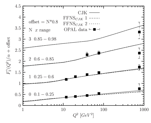
Figure 6: As in Fig. 5 for $F_{2}^{\gamma}(x,Q^{2})$/$\alpha$, averaged over four different $x$ ranges.

Apart from this direct comparison with the photon structure function $F_{2}^{\gamma}$ data, we perform another comparison, this time with LEP data that were not used directly in our analysis. Figures 5 and 6 present our predictions for the $F_{2}^{\gamma}(x,Q^{2})$, averaged over various $x$ regions, compared with the recent OPAL data [24]. Like in our previous analysis we see that all FFNS type predictions (including GRS LO and SaS1D parametrizations) are similar and fairly well describe the experimental data. Moreover, again the CJK model, alike the CJKL model, slightly differs from other fits. However, this difference is much smaller now and gives better agreement with the data.

We observe that for the case of the medium-$x$ range, $0.1<x<0.6$, there are small differences between the CJK and both FFNS models at very low $Q^{2}$, where there are no experimental data, and at large $Q^{2}$ where a slightly better agreement between the CJK model prediction and the OPAL data is found. Comparing with the plot in Fig. 6 we see that larger values of the $F_{2}^{\gamma}(x,Q^{2})$ obtained for the CJK model are originated at lower values of $x$ in the considered range, as one could expect from Figs. 1–4.

4.2 Parton densities

It is very instructive to discuss the parton densities obtained in the CJK and FFNS_CJK fits. We choose to present results for medium- and high-$x$ at $Q^{2}=10$ GeV², see Fig. 7. In Figs. 8–10 we show the up-, and charm-quark and gluon densities for various $Q^{2}$ values. First we observe that parton distributions obtained in various models are very similar, except that of course there are no heavy-quark distributions in FFNS-type approaches. In the case of the CJK models, due to the introduction of the $\chi_{h}$ variable, the $c^{\gamma}(x,Q^{2})$ and $b^{\gamma}(x,Q^{2})$ densities vanish not at $x=1$, as in the case of the GRV LO [5] and SaS1D parametrizations, but as they should at the kinematic threshold. Moreover, the CJK heavy-quark densities at low $x$ are larger than the corresponding densities obtained in other parametrizations. This is a feature that can be observed in a wide range of $Q^{2}$ values in Fig. 9.

We notice that our new parton densities have all similar shapes to the corresponding old CJKL distributions. Though, in the medium- and high-$x$ regions they have slightly higher values. On contrary, at very low $x$ values CJKL densities are greater than the new ones, opposite case occurs in the $10^{-3}<x<10^{-2}$ region. In the case of the gluon density we find that all new lines are much steeper at high-$x$ than the predictions of our previous models and the GRV LO and SaS1D parametrizations.

4.3 Comparison with $F^{\gamma}_{2,c}$

We compare the individual contributions included in the CJK model relevant for our predictions of the $F_{2,c}^{\gamma}$. Results from the CJK fit are presented in Fig. 11 for $Q^{2}=5,20,100$ and 1000 GeV². Almost all the contributing terms vanish in the $W\to 2m_{c}$ threshold in a natural way due to the introduction of the $\chi_{h}$ variable. The only exception is the one subtraction term, namely $F_{2,c}|_{dir,sub}$ which dominates near the highest kinematically allowed $x$ value and vanishes only due to the extra condition, $F_{2,c}|_{dir,sub}=0$ for $\chi_{h}>1$, we imposed. The direct (Bethe-Heitler) term is important in the medium-$x$ range. Its shape resembles the valence-type distribution. The charm-quark density contribution, i.e. the term $2xe_{c}^{2}c^{\gamma}(x,Q^{2})$, is important in the whole kinematically available $x$ range and dominates the $F_{2,c}^{\gamma}$ for small $x$. In this region also both resolved-photon contributions increase with decreasing $x$, but to great extent they cancel each other.

Finally we see that imposing the improved positivity condition $F_{2,h}^{\gamma}>F_{2,h}(x,Q^{2})^{\gamma}(x,Q^{2})|_{dir}+F_{2,h}^{\gamma}(x,Q^{2})|_{res}$ on the heavy-quark contributions to the $F_{2}^{\gamma}(x,Q^{2})$ results in correct threshold behaviour of the total $F_{2,c}$ function. Unlike in the case of the CJKL fit, the $F_{2,h}^{\gamma}$ and its contributions vanish at the same high $x$ value.

A good test of the charm-quark contributions is provided by the OPAL measurement of the $F_{2,c}^{\gamma}$, obtained from the inclusive production of $D^{*\pm}$ mesons in photon-photon collisions [34]. The averaged $F_{2,c}^{\gamma}$ has been determined in the two $x$ bins. These data points are compared to the predictions of the CJK and FFNS_CJK models and GRS LO and SaS1D parametrizations in Fig. 12.

Our first observation is the following: our models containing the resolved-photon contribution, $F_{2,h}^{\gamma}(x,Q^{2})|_{res}$ (FFNS_CJK2 and the CJK model) agree better with the low-$x$ experimental point than other predictions. The GRS LO and SaS1D parametrizations also include the resolved-photon term but in their case the gluon density increased less steep than our models predict, as was already mentioned. Their $F_{2,c}^{\gamma}$ lines lie below the results of our new fits but higher than the FFNS_CJK1 curve, given solely by the direct Bethe-Heitler contribution.

The CJK model overshoots the experimental point at high $x$ while other predictions agree with it within its uncertainty bounds. Taking into account both data points we conclude that the best agreement with the experimental results is provided by the FFNS_CJK2 model.

4.4 Gluon densities at HERA

We also checked that the gluon densities of CJK and FFNS_CJK models agree with the H1 measurement of the $G^{\gamma}$ distribution performed at $Q^{2}=74$ GeV² [35]. As can be seen in Fig. 13 all models predict gluon densities that lie above the one provided by the GRV LO parametrization, which gave so far best agreement with the H1 data. Further comparison of our gluon densities to the H1 data cannot be performed in a fully consistent way, since the GRV LO proton and photon parametrization were used in the experiment in order to extract such gluon density.

4.5 The uncertainties of the CJK parton distributions

Let us now present the main results of an analysis of the CJK parton distribution uncertainties described in detail in [3].

During the last two years numerous analysis of the uncertainties of the proton parton densities resulting from the experimental data errors appeared. The CTEQ Collaboration in a series of publications, [7, 8, 9], developed and applied a new method of their treatment significantly improving the traditional approach to this matter. Later the same approach has been applied by the MRST group in [10]. The method, denoted as Hessian method, bases on the Hessian formalism. We applied it for the very first time to the case of the photon parton distributions [3, 2].

The uncertainties analysis was performed for the CJK photon parametrization only. The set of the best values of parameters $\kappa,\alpha,\beta$ and $N_{v}$, corresponding to the minimal $\chi^{2}$ of the global fit, $\chi_{0}^{2}$ (table 1), is denoted as the $S^{0}$ parametrization. Using the Hessian method we created an additional basis of the test parametrizations of the CJK parton densities, $\{S_{k}^{\pm},k=1,\cdots,4\}$, where 4 corresponds to the number of free parameters of the model. The set $\{S_{k}^{\pm}\}$ allows for the calculation of the uncertainty of any physical observable $X$ depending on the parton densities. Its best value is given as $X(S^{0})$. The uncertainty of $X$, for a displacement from the parton densities minimum by $\Delta\chi^{2}=T^{2}$ (T - the tolerance parameter) can be calculated with a very simple expression (named as master equation by the CTEQ Collaboration)

$$\Delta X=\frac{T}{2t}\left(\sum_{k=1}^{d}[X(S_{k}^{+})-X(S_{k}^{-})]^{2}\right)^{\frac{1}{2}},$$ (16)

where parameter $t=5$ in that particular case. After a detailed test of the allowed deviation of the global fit from the minimum, we found that $T$ should lie in the range $5\sim 10$ [3]. Note that having calculated $\Delta X$ for one value of the tolerance parameter $T$ we can obtain the uncertainty of $X$ for any other $T$ by simple scaling of $\Delta X$. This way sets of $\{S_{k}^{\pm}\}$ parton densities give us a perfect tool for studying of the uncertainties of other physical quantities. One of such quantities can be the parton densities themselves.

In Figure 14 the up-, strange- and charm-quark and gluon densities calculated in the FFNS_CJK models and the GRV LO, GRS LO and SaS1D parametrizations are compared with the CJK predictions. We plot for $Q^{2}=10$ and 100 GeV² the ratios $q^{\gamma}(\mathrm{Other\>model})/q^{\gamma}(\mathrm{CJK})$ and $q^{\gamma}(\mathrm{Other\>parametrization})/q^{\gamma}(\mathrm{CJK})$ of the parton $q^{\gamma}$ densities calculated in the CJK model and other models (or parametrizations). Solid lines show the CJK fit uncertainties for $\Delta\chi^{2}=25$ computed with the $\{S_{k}^{\pm}\}$ test parametrizations. First we notice that predictions of FFNS_CJK models in the case of all parton distributions lie between the lines of the CJK uncertainties. There is only one range of $x$, namely $0.01^{<}\hskip-7.11317pt_{\sim}x^{<}\hskip-7.11317pt_{\sim}0.1$ at $Q^{2}=10$ GeV² where the up- and down-quark densities predicted by the FFNS_CJK 1 fit go slightly beyond the uncertainty band. This indicates that the choice of $\Delta\chi^{2}=25$ agrees with the differences among our four models. Moreover, the GRV LO parametrization predictions are nearly contained within the CJK model uncertainties. Obviously, that is not the case, for the heavy-quark densities. The SaS1D results differ very substantially from the CJK ones. Next, we observe that, as expected, the up-quark distribution is the one best constrained by the experimental data, while the greatest uncertainties are connected with the gluon densities. In the case of $u^{\gamma}$, the $\Delta\chi^{2}=25$ band widens in the small $x$ region. Alike in the case of other quark uncertainties it shrinks at high $x$, this is due to the large $u$-quark density in the photon at high $x$. On contrary the gluon distributions are least constrained at the region of $x\to 1$. Finally we observe that all uncertainties become slightly smaller when we go to higher $Q^{2}$ from 10 to 100 GeV² (not shown).

5 Summary

We enlarged and improved our previous analysis [1]. Here we performed 3 new global fits to the $F_{2}^{\gamma}(x,Q^{2})$ data, excluding the TPC2$\gamma$ experiment. Two additional models were analysed. New fits gave $\chi^{2}$ per degree of freedom, 1.5-1.7, about 0.25 better than the old results. All features of the CJKL model, such as the shape of the heavy-quark distributions, good description of the LEP data on the $Q^{2}$ dependence of the $F_{2}^{\gamma}$ and on $F_{2,c}^{\gamma}$ are preserved. We checked that the gluon densities of our models agree with the H1 measurement of the $G^{\gamma}$ distribution performed at $Q^{2}=74$ GeV² [35].

An analysis of the uncertainties of the CJK parton distributions due to the experimental errors based on the Hessian method was performed for the very first time for the photon [3, 2]. We constructed set of test parametrizations for the CJK model. It allows to computate uncertainties of any physical quantity depending on the real photon parton densities.

Fortran parametrization programs for all models, obtained through parametrization of the fit results on the grid, can be obtained from the web-page [27]. Set of the data used in the fits is also given there.

Figure 1: Predictions for the $F_{2}^{\gamma}(x,Q^{2})/\alpha$ for the CJK and FFNS_CJK models compared with the experimental data [14, 15, 16, 17, 18, 19, 20, 21, 22, 23, 24], for small and medium $Q^{2}$ as a function of $x$ (logarithmic scale). If a few values of $Q^{2}$ are displayed in the panel, the average of the smallest and biggest $Q^{2}$ was taken in the computation.

Figure 2: The same as in Fig. 1, for $Q^{2}\gtrsim 20\mathrm{GeV}^{2}$.

Figure 3: The same as in Fig. 1 for a linear scale in $x$.

Figure 4: The same as in Fig. 2 for a linear scale in $x$.

Figure 5: Comparison of the recent OPAL data [24] for the $Q^{2}$-dependence of the averaged over $0.1<x<0.6$ $F_{2}^{\gamma}/\alpha$ with the predictions of the CJK and FFNS_CJK models.

Figure 7: Comparison of the parton densities predicted by various models at $Q^{2}=10$ GeV², as a function of $x$.

Figure 8: Comparison of the up-quark density at four values of $Q^{2}$ in the CJK and FFNS_CJK models, as a function of $x$.

Figure 9: The same as in Fig. 8 for the gluon density.

Figure 10: The same as in Fig. 8 for the charm-quark density.

Figure 11: Comparison of various contributions to the photon structure function $F_{2,c}^{\gamma}(x,Q^{2})/\alpha$ in the CJK model for $Q^{2}=5,20,100$ and 1000 GeV².

Figure 12: Comparison of the structure function $F_{2,c}^{\gamma}(x,Q^{2})/\alpha$ calculated in the CJK and FFNS_CJK models and in GRS LO [30] and SaS1D [33] parametrizations with the OPAL measurement [34].

Figure 13: Comparison of the gluon distribution obtained in the H1 measurement performed at $Q^{2}=74$ GeV² [35] with the predictions of the CJK, FFNS_CJK1 & 2 models and GRV LO [5], GRS LO [30] and SaS1D [33] parametrizations with the OPAL measurement [34].

Figure 14: Parton densities calculated in FFNS_CJK models and GRV LO [5], GRS LO [30] and SaS1D [33] parametrizations compared with the CJK predictions. We plot for $Q^{2}=10$ GeV² the $q^{\gamma}(\mathrm{Other\>parametrization})/q^{\gamma}(\mathrm{CJK})$ ratios of the parton density calculated in the CJK model and its values obtained with other models and parametrizations. Solid lines show the CJK fit uncertainties for $\Delta\chi^{2}=25$ computed with the set of the $\{S_{k}^{\pm}\}$ test parametrizations.

References

- [1] F.Cornet, P.Jankowski, M.Krawczyk and A.Lorca, Phys. Rev D68, 014010 (2003)
- [2] F. Cornet, P. Jankowski and M. Krawczyk, Nucl.Phys. (Proc. Suppl.) B126, 28 (2004), arXiv:hep-ph/0310029
- [3] P. Jankowski, IFT-2003-31, accepted by JHEP, arXiv:hep-ph/0312056
-
[4]
S.Kretzer, C.Schmidt and W.Tung,
Proceedings of New Trends in HERA Physics,
Ringberg Castle, Tegernsee, Germany, 17-22
Jun 2001, Published in J. Phys. G28, 983 (2002);
S. Kretzer, H.L. Lai, F.I. Olness and W.K. Tung, arXiv: hep-ph/0307022 - [5] M.Glück, E.Reya and A.Vogt, Phys. Rev. D46, 1973 (1992)
- [6] M.Glück, E.Reya and M.Stratmann, Phys. Rev. D51, 3220 (1995)
- [7] J.Pumplin, D.R.Stump and W.K.Tung, Phys. Rev. D65, 014011 (2002)
- [8] J.Pumplin et al., Phys. Rev. D65, 014013 (2002)
- [9] J.Pumplin et al., JHEP 0207, 012 (2002)
- [10] A.D.Martin, R.G.Roberts, W.J.Stirling and R.S.Thorne, Eur. Phys. J. C28, 455 (2003)
- [11] G. Parisi, Proceedings of 11th Rencontres de Moriond 1976, editor J. Tran Thanh Van; G. Altarelli and G. Parisi, Nucl. Phys. B126, 298 (1997);
- [12] J.H.Field, VIIIth International Workshop on Photon-Photon Collisions, Shoresh, Jerusalem Hills Israel, 1988; U. Maor, Acta Phys. Polonica B19, 623 (1988); Ch. Berger and W. Wagner, Phys. Rep. 146, 1 (1987)
- [13] Particle Data Group (D.E. Groom et al.), Eur. Phys. J. C15, 1 (2000)
- [14] CELLO Collaboration, H. J. Behrend et al., Phys. Lett. B126, 391 (1983); in Proceedings of the XXVth International Conference on High Energy Physics, Singapore, 1990, edited by K. K. Phua and Y. Yamaguchi (World Scientific, Singapore, 1991).
- [15] PLUTO Collaboration, Ch. Berger et al., Phys. Lett. B142 111 (1984); Nucl. Phys. B281, 365 (1987).
- [16] JADE Collaboration, W. Bartel et al., Z. Phys. C24, 231 (1984).
- [17] TASSO Collaboration, M. Althoff et al., Z. Phys. C31, 527 (1986).
- [18] TOPAZ Collaboration, K. Muramatsu et al., Phys. Lett. B332, 477 (1994).
- [19] AMY Collaboration, S. K. Sahu et al., Phys. Lett. B346, 208 (1995); T. Kojima et al., ibid. B400, 395 (1997).
- [20] DELPHI Collaboration, P. Abreu et al., Z. Phys. C69, 223 (1996); I. Tyapkin, Proceedings of Workshop on Photon Interaction and the Photon Structure, Lund, Sweden, 1998, edited by G. Jarlskog and T. Sjöstrand, to appear in the Proceedings of International Conference on the Structure and Interactions of the Photon and 14th International Workshop on Photon-Photon Collisions (Photon 2001), Ascona, Switzerland, 2001.
- [21] L3 Collaboration, M. Acciarri et al., Phys. Lett. B436, 403 (1998); ibid. B447, 147 (1999); ibid. B483, 373 (2000).
- [22] ALEPH Collaboration, R. Barate et al., Phys. Lett. B458, 152 (1999); K. Affholderbach et al., Proceedings of the International Europhysics Conference on High Energy Physics, Tampere, Finland, 1999, Nucl. Phys. Proc. Suppl. B86, 122 (2000).
- [23] OPAL Collaboration, K. Ackerstaff et al., Z. Phys. C74, 33 (1997); Phys. Lett. B411, 387 (1997); G. Abbiendi et al., Eur. Phys. J. C18, 15 (2000).
- [24] OPAL Collaboration, G. Abbiendi et al., Phys. Lett. B533, 207 (2002).
- [25] TPC/ Collaboration, H. Aihara et al., Z. Phys. C34, 1 (1987); J. S. Steinman, Ph.D. Thesis, UCLA-HEP-88-004, Jul 1988.
- [26] S. Albino, M. Klasen and S. Söldner-Rembold, Phys. Rev. Lett. 89, 122004 (2002).
-
[27]
http://www.fuw.edu.pl/
~pjank/param.html - [28] We thank Mariusz Przybycień for pointing this problem to us.
- [29] F.James and M.Roos, Comput. Phys. Commun. 10, 343 (1975)
- [30] M.Glück, E.Reya and I.Schienbein, Phys. Rev. D60, 054019 (1999), Erratum-ibid. D62, 019902 (2000)
- [31] M.Glück, E.Reya and A.Vogt, Z. Phys. C53, 651 (1992)
- [32] B.L. Ioffe, arXiv: hep-ph/0209254
- [33] G.A.Schuler and T.Sjöstrand, Z. Phys. C68, 607 (1995); Phys. Lett. B376, 193 (1996)
- [34] OPAL Collaboration, G.Abbiendi et al., Phys. Lett. B539, 13 (2002)
- [35] H1 Collaboration, C.Adloff et al., Phys. Lett. B483, 36 (2000)