Neutrinos in Cosmology

Abstract

The current status of neutrino cosmology is reviewed, from the question of neutrino decoupling and the presence of sterile neutrinos to the effects of neutrinos on the cosmic microwave background and large scale structure. Particular emphasis is put on cosmological neutrino mass measurements.

1 Introduction

Next to photons neutrinos are the most abundant particles in the universe. This means they have a profound impact on many different aspects of cosmology, from the question of leptogenesis in the very early universe, over big bang nucleosynthesis, to late time structure formation. In the present review I focus mainly on late-time aspects of neutrino cosmology, and particularly on issues relevant to cosmological bounds on the neutrino mass.

The absolute value of neutrino masses are very difficult to measure experimentally. On the other hand, mass differences between neutrino mass eigenstates, $(m_{1},m_{2},m_{3})$, can be measured in neutrino oscillation experiments.

The combination of all currently available data suggests two important mass differences in the neutrino mass hierarchy. The solar mass difference of $\delta m_{12}^{2}\simeq 7\times 10^{-5}$ eV² and the atmospheric mass difference $\delta m_{23}^{2}\simeq 2.6\times 10^{-3}$ eV² [3, 1, 2].

In the simplest case where neutrino masses are hierarchical these results suggest that $m_{1}\sim 0$, $m_{2}\sim\delta m_{\rm solar}$, and $m_{3}\sim\delta m_{\rm atmospheric}$. If the hierarchy is inverted [4, 5, 6, 7, 8, 9] one instead finds $m_{3}\sim 0$, $m_{2}\sim\delta m_{\rm atmospheric}$, and $m_{1}\sim\delta m_{\rm atmospheric}$. However, it is also possible that neutrino masses are degenerate [10, 11, 12, 13, 14, 15, 16, 17, 18, 19, 20], $m_{1}\sim m_{2}\sim m_{3}\gg\delta m_{\rm atmospheric}$, in which case oscillation experiments are not useful for determining the absolute mass scale.

Experiments which rely on kinematical effects of the neutrino mass offer the strongest probe of this overall mass scale. Tritium decay measurements have been able to put an upper limit on the electron neutrino mass of 2.3 eV (95% conf.) [21]. However, cosmology at present yields an much stronger limit which is also based on the kinematics of neutrino mass.

Very interestingly there is also a claim of direct detection of neutrinoless double beta decay in the Heidelberg-Moscow experiment [22, 23], corresponding to an effective neutrino mass in the $0.1-0.9$ eV range. If this result is confirmed then it shows that neutrino masses are almost degenerate and well within reach of cosmological detection in the near future.

Another important question which can be answered by cosmological observations is how large the total neutrino energy density is. Apart from the standard model prediction of three light neutrinos, such energy density can be either in the form of additional, sterile neutrino degrees of freedom, or a non-zero neutrino chemical potential.

The paper is divided into sections in the following way: In section 2 I review the present cosmological data which can be used for analysis of neutrino physics. In section 3 I discuss neutrino physics around the epoch of neutrino decoupling at a temperature of roughly 1 MeV, including the relation between neutrinos and Big Bang nucleosynthesis. Section 4 discusses neutrinos as dark matter particles, including mass constraints on light neutrinos, and sterile neutrino dark matter. Section 5 contains a relatively short review of neutrino physics in the very early universe from the perspective of leptogenesis. Finally, section 6 contains a discussion.

2 Cosmological data

Large Scale Structure (LSS) –

At present there are two large galaxy surveys of comparable size, the Sloan Digital Sky Survey (SDSS) [24, 25] and the 2dFGRS (2 degree Field Galaxy Redshift Survey) [26]. Once the SDSS is completed in 2005 it will be significantly larger and more accurate than the 2dFGRS. At present the two surveys are, however, comparable in precision.

Cosmic Microwave Background (CMB) –

The temperature fluctuations are conveniently described in terms of the spherical harmonics power spectrum $C_{T,l}\equiv\langle|a_{lm}|^{2}\rangle$, where $\frac{\Delta T}{T}(\theta,\phi)=\sum_{lm}a_{lm}Y_{lm}(\theta,\phi)$. Since Thomson scattering polarizes light, there are also power spectra coming from the polarization. The polarization can be divided into a curl-free $(E)$ and a curl $(B)$ component, yielding four independent power spectra: $C_{T,l}$, $C_{E,l}$, $C_{B,l}$, and the $T$-$E$ cross-correlation $C_{TE,l}$.

The WMAP experiment has reported data only on $C_{T,l}$ and $C_{TE,l}$ as described in Refs. [27, 28, 29, 30, 31, 32]. Foreground contamination has already been subtracted from their published data.

In addition to the WMAP experiment there are a number of other current CMB experiments, both ground and balloon based. Wang et al. [34] have provided a compilation of various data sets, and in addition to these there is the ACBAR experiment [33] which has measured the CMB at small scales.

Other data –

Apart from CMB and LSS data there are a number of other cosmological measurements of importance to neutrino cosmology. One is the measurement of the Hubble constant by the HST Hubble Key Project, $H_{0}=72\pm 8~{}{\rm km}~{}{\rm s}^{-1}~{}{\rm Mpc}^{-1}$ [35].

The constraint on the matter density coming from measurements of distant type Ia supernovae is also important for neutrino physics. The most recent result is from the Supernova Cosmology Project [36] and yields $\Omega_{m}=0.25^{+0.07}_{-0.06}$ (statistical) $\pm 0.04$ (identified systematics).

3 Neutrino Decoupling

3.1 Standard model

In the standard model neutrinos interact via weak interactions with $e^{+}$ and $e^{-}$. In the absence of oscillations neutrino decoupling can be followed via the Boltzmann equation for the single particle distribution function [37]

$$\frac{\partial f}{\partial t}-Hp\frac{\partial f}{\partial p}=C_{\rm coll},$$ (1)

where $C_{\rm coll}$ represents all elastic and inelastic interactions. In the standard model all these interactions are $2\leftrightarrow 2$ interactions in which case the collision integral for process $i$ can be written

$$C_{\rm coll,i}(f_{1}) = \frac{1}{2E_{1}}\int\frac{d^{3}{\bf p}_{2}}{2E_{2}(2\pi)^{3}}\frac{d^{3}{\bf p}_{3}}{2E_{3}(2\pi)^{3}}\frac{d^{3}{\bf p}_{4}}{2E_{4}(2\pi)^{3}}$$ (2)

$$\,\,\times(2\pi)^{4}\delta^{4}(p_{1}+p_{2}-p_{3}+p_{4})\Lambda(f_{1},f_{2},f_{3},f_{4})S|M|^{2}_{12\to 34,i},$$

where $S|M|^{2}_{12\to 34,i}$ is the spin-summed and averaged matrix element including the symmetry factor $S=1/2$ if there are identical particles in initial or final states. The phase-space factor is $\Lambda(f_{1},f_{2},f_{3},f_{4})=f_{3}f_{4}(1-f_{1})(1-f_{2})-f_{1}f_{2}(1-f_{3})(1-f_{4})$.

The matrix elements for all relevant processes can for instance be found in Ref. [38]. If Maxwell-Boltzmann statistics is used for all particles, and neutrinos are assumed to be in complete scattering equilbrium so that they can be represented by a single temperature, then the collision integral can be integrated to yield the average annihilation rate for a neutrino

$$\Gamma=\frac{16G_{F}^{2}}{\pi^{3}}(g_{L}^{2}+g_{R}^{2})T^{5},$$ (3)

where

$$g_{L}^{2}+g_{R}^{2}=\cases{\sin^{4}\theta_{W}+(\frac{1}{2}+\sin^{2}\theta_{W})^{2}&for $\nu_{e}$\cr\sin^{4}\theta_{W}+(-\frac{1}{2}+\sin^{2}\theta_{W})^{2}&for $\nu_{\mu,\tau}$}.$$ (4)

This rate can then be compared with the Hubble expansion rate

$$H=1.66g_{*}^{1/2}\frac{T^{2}}{M_{\rm Pl}}$$ (5)

to find the decoupling temperature from the criterion $\left.H=\Gamma\right|_{T=T_{D}}$. From this one finds that $T_{D}(\nu_{e})\simeq 2.4$ MeV, $T_{D}(\nu_{\mu,\tau})\simeq 3.7$ MeV, when $g_{*}=10.75$, as is the case in the standard model.

This means that neutrinos decouple at a temperature which is significantly higher than the electron mass. When $e^{+}e^{-}$ annihilation occurs around $T\sim m_{e}/3$, the neutrino temperature is unaffected whereas the photon temperature is heated by a factor $(11/4)^{1/3}$. The relation $T_{\nu}/T_{\gamma}=(4/11)^{1/3}\simeq 0.71$ holds to a precision of roughly one percent. The main correction comes from a slight heating of neutrinos by $e^{+}e^{-}$ annihilation, as well as finite temperature QED effects on the photon propagator [39, 40, 41, 42, 43, 44, 38, 45, 46, 47, 48, 49, 50, 51].

3.2 Big Bang nucleosynthesis and the number of neutrino species

Shortly after neutrino decoupling the weak interactions which keep neutrons and protons in statistical equilibrium freeze out. Again the criterion $\left.H=\Gamma\right|_{T=T_{\rm freeze}}$ can be applied to find that $T_{\rm freeze}\simeq 0.5g_{*}^{1/6}$ MeV [37].

Eventually, at a temperature of roughly 0.2 MeV deuterium starts to form, and very quickly all free neutrons are processed into ⁴He. The final helium abundance is therefore roughly given by

$$Y_{P}\simeq\left.\frac{2n_{n}/n_{p}}{1+n_{n}/n_{p}}\right|_{T\simeq 0.2\,\,{\rm MeV}}.$$ (6)

$n_{n}/n_{p}$ is determined by its value at freeze out, roughly by the condition that $n_{n}/n_{p}|_{T=T_{\rm freeze}}\sim e^{-(m_{n}-m_{p})/T_{\rm freeze}}$.

Since the freeze-out temperature is determined by $g_{*}$ this in turn means that $g_{*}$ can be inferred from a measurement of the helium abundance. However, since $Y_{P}$ is a function of both $\Omega_{b}h^{2}$ and $g_{*}$ it is necessary to use other measurements to constrain $\Omega_{b}h^{2}$ in order to find a bound on $g_{*}$. One customary method for doing this has been to use measurements of primordial deuterium to infer $\Omega_{b}h^{2}$ and from that calculate a bound on $g_{*}$. Usually such bounds are expressed in terms of the equivalent number of neutrino species, $N_{\nu}\equiv\rho/\rho_{\nu_{0}}$, instead of $g_{*}$. The exact value of the bound is quite uncertain because there are different and inconsistent measurements of the primordial helium abundance (see for instance Ref. [52] for a discussion of this issue). The most recent analyses are [52] where a value of $1.7\leq N_{\nu}\leq 3.0$ (95% C.L.) was found and [53] which found the result $N_{\nu}=2.5^{+1.1}_{-0.9}$. The difference in these results can be attributed to different assumptions about uncertainties in the primordial helium abundance.

Another interesting parameter which can be constrained by the same argument is the neutrino chemical potential, $\xi_{\nu}=\mu_{\nu}/T$ [54, 55, 56, 57]. At first sight this looks like it is completely equivalent to constraining $N_{\nu}$. However, this is not true because a chemical potential for electron neutrinos directly influences the $n-p$ conversion rate. Therefore the bound on $\xi_{\nu_{e}}$ from BBN alone is relatively stringent ($-0.1\,\hbox to0.0pt{\lower 3.5pt\hbox{$\mathchar 0\relax\sim$}\hss}\raise 1.0pt\hbox{$<$}\,\xi_{\nu_{e}}\,\hbox to0.0pt{\lower 3.5pt\hbox{$\mathchar 0\relax\sim$}\hss}\raise 1.0pt\hbox{$<$}\,1$ [54]) compared to that for muon and tau neutrinos ($\left|\xi_{\nu_{\mu,\tau}}\right|\,\hbox to0.0pt{\lower 3.5pt\hbox{$\mathchar 0\relax\sim$}\hss}\raise 1.0pt\hbox{$<$}\,7$ [54]). However, as will be seen in the next section, neutrino oscillations have the effect of almost equilibrating the neutrino chemical potentials prior to BBN, completely changing this conclusion.

3.3 The number of neutrino species - joint CMB and BBN analysis

The BBN bound on the number of neutrino species presented in the previous section can be complemented by a similar bound from observations of the CMB and large scale structure. The CMB depends on $N_{\nu}$ mainly because of the early Integrated Sachs Wolfe effect which increases fluctuation power at scales slightly larger than the first acoustic peak. The large scale structure spectrum depends on $N_{\nu}$ because the scale of matter-radiation equality is changed by varying $N_{\nu}$.

Several recent papers have analyzed WMAP and 2dF data for bounds on $N_{\nu}$ [59, 58, 60, 52, 53], and some of the bounds are listed in Table 1. Recent analyses combining BBN, CMB, and large scale structure data can be found in [58, 52], and these results are also listed in Table 1.

Common for all the bounds is that $N_{\nu}=0$ is ruled out by both BBN and CMB/LSS. This has the important consequence that the cosmological neutrino background has been positively detected, not only during the BBN epoch, but also much later, during structure formation.

Table 1: Various recent limits on the effective number of neutrino species, as well as the data used.

Ref.	Bound on $N_{\nu}$	Data used
Crotty et al. [59]	$1.4\leq N_{\nu}\leq 6.8$	CMB, LSS
Hannestad [58]	$0.9\leq N_{\nu}\leq 7.0$	CMB, LSS
Pierpaoli [60]	$1.9\leq N_{\nu}\leq 6.62$	CMB, LSS
Barger et al. [52]	$0.9\leq N_{\nu}\leq 8.3$	CMB
Hannestad [58]	$2.3\leq N_{\nu}\leq 3.0$	CMB, LSS, BBN
Barger et al. [52]	$1.7\leq N_{\nu}\leq 3.0$	CMB, BBN

3.4 The effect of oscillations

In the previous section the one-particle distribution function, $f$, was used to describe neutrino evolution. However, for neutrinos the mass eigenstates are not equivalent to the flavour eigenstates because neutrinos are mixed. Therefore the evolution of the neutrino ensemble is not in general described by the three scalar functions, $f_{i}$, but rather by the evolution of the neutrino density matrix, $\rho\equiv\psi\psi^{\dagger}$, the diagonal elements of which correspond to $f_{i}$.

For three-neutrino oscillations the formalism is quite complicated. However, the difference in $\Delta m_{12}$ and $\Delta m_{23}$, as well as the fact that $\sin 2\theta_{13}\ll 1$ means that the problem effectively reduces to a $2\times 2$ oscillation problem in the standard model. A detailed account of the physics of neutrino oscillations in the early universe is outside the scope of the present paper, however an excellent and very thorough review can be found in Ref. [61]

Without oscillations it is possible to compensate a very large chemical potential for muon and/or tau neutrinos with a small, negative electron neutrino chemical potential [54]. However, since neutrinos are almost maximally mixed a chemical potential in one flavour can be shared with other flavours, and the end result is that during BBN all three flavours have almost equal chemical potential. This in turn means that the bound on $\nu_{e}$ applies to all species so that [62, 63, 64, 65, 66].

$$|\xi_{i}|=\frac{|\eta_{i}|}{T}\,\hbox to0.0pt{\lower 3.5pt\hbox{$\mathchar 0\relax\sim$}\hss}\raise 1.0pt\hbox{$<$}\,0.15$$ (7)

for $i=e,\mu,\tau$.

In models where sterile neutrinos are present even more remarkable oscillation phenomena can occur. However, I do not discuss this possibility further, except for the possibility of sterile neutrino warm dark matter, and instead refer to the review [61].

3.5 Low reheating temperature and neutrinos

In most models of inflation the universe enters the normal, radiation dominated epoch at a reheating temperature, $T_{\rm RH}$, which is of order the electroweak scale or higher. However, in principle it is possible that this reheating temperature is much lower, of order MeV. This possibility has been studied many times in the literature, and a very general bound of $T_{\rm RH}\,\hbox to0.0pt{\lower 3.5pt\hbox{$\mathchar 0\relax\sim$}\hss}\raise 1.0pt\hbox{$>$}\,1$ MeV has been found [67, 68, 69, 70]

This very conservative bound comes from the fact that the light element abundances produced by big bang nucleosynthesis disagree with observations if the universe if matter dominated during BBN. However, a somewhat more stringent bound can be obtained by looking at neutrino thermalization during reheating. If a scalar particle is responsible for reheating then direct decay to neutrinos is suppressed because of the necessary helicity flip. This means that if the reheating temperature is too low neutrinos never thermalize. If this is the case then BBN predicts the wrong light element abundances. However, even if the heavy particle has a significant branching ratio into neutrinos there are problems with BBN. The reason is that neutrinos produced in decays are born with energies which are much higher than thermal. If the reheating temperature is too low then a population of high energy neutrinos will remain and also lead to conflict with observed light element abundances. A recent analysis showed that in general the reheating temperature cannot be below roughly 4 MeV [71].

4 Neutrino Dark Matter

Neutrinos are a source of dark matter in the present day universe simply because they contribute to $\Omega_{m}$. The present temperature of massless standard model neutrinos is $T_{\nu,0}=1.95\,K=1.7\times 10^{-4}$ eV, and any neutrino with $m\gg T_{\nu,0}$ behaves like a standard non-relativistic dark matter particle.

The present contribution to the matter density of $N_{\nu}$ neutrino species with standard weak interactions is given by

$$\Omega_{\nu}h^{2}=N_{\nu}\frac{m_{\nu}}{92.5\,{\rm eV}}$$ (8)

Just from demanding that $\Omega_{\nu}\leq 1$ one finds the bound [72, 73]

$$m_{\nu}\,\hbox to0.0pt{\lower 3.5pt\hbox{$\mathchar 0\relax\sim$}\hss}\raise 1.0pt\hbox{$<$}\,\frac{46\,{\rm eV}}{N_{\nu}}$$ (9)

4.1 The Tremaine-Gunn bound

If neutrinos are the main source of dark matter, then they must also make up most of the galactic dark matter. However, neutrinos can only cluster in galaxies via energy loss due to gravitational relaxation since they do not suffer inelastic collisions. In distribution function language this corresponds to phase mixing of the distribution function [74]. By using the theorem that the phase-mixed or coarse grained distribution function must explicitly take values smaller than the maximum of the original distribution function one arrives at the condition

$$f_{\rm CG}\leq f_{\nu,{\rm max}}=\frac{1}{2}$$ (10)

Because of this upper bound it is impossible to squeeze neutrino dark matter beyond a certain limit [74]. For the Milky Way this means that the neutrino mass must be larger than roughly 25 eV if neutrinos make up the dark matter. For irregular dwarf galaxies this limit increases to 100-300 eV [75, 76], and means that standard model neutrinos cannot make up a dominant fraction of the dark matter. This bound is generally known as the Tremaine-Gunn bound.

Note that this phase space argument is a purely classical argument, it is not related to the Pauli blocking principle for fermions (although, by using the Pauli principle $f_{\nu}\leq 1$ one would arrive at a similar, but slightly weaker limit for neutrinos). In fact the Tremaine-Gunn bound works even for bosons if applied in a statistical sense [75], because even though there is no upper bound on the fine grained distribution function, only a very small number of particles reside at low momenta (unless there is a condensate). Therefore, although the exact value of the limit is model dependent, limit applies to any species that was once in thermal equilibrium. A notable counterexample is non-thermal axion dark matter which is produced directly into a condensate.

4.2 Neutrino hot dark matter

A much stronger upper bound on the neutrino mass than the one in Eq. (9) can be derived by noticing that the thermal history of neutrinos is very different from that of a WIMP because the neutrino only becomes non-relativistic very late.

In an inhomogeneous universe the Boltzmann equation for a collisionless species is [77]

$$L[f]=\frac{Df}{D\tau}=\frac{\partial f}{\partial\tau}+\frac{dx^{i}}{d\tau}\frac{\partial f}{\partial x^{i}}+\frac{dq^{i}}{d\tau}\frac{\partial f}{\partial q^{i}}=0,$$ (11)

where $\tau$ is conformal time, $d\tau=dt/a$, and $q^{i}=ap^{i}$ is comoving momentum. The second term on the right-hand side has to do with the velocity of the distribution in a given spatial point and the third term is the cosmological momentum redshift.

Following Ma and Bertschinger [77] this can be rewritten as an equation for $\Psi$, the perturbed part of $f$

$$f(x^{i},q^{i},\tau)=f_{0}(q)\left[1+\Psi(x^{i},q^{i},\tau)\right]$$ (12)

In synchronous gauge that equation is

$$\frac{1}{f_{0}}[f]=\frac{\partial\Psi}{\partial\tau}+i\frac{q}{\epsilon}\mu\Psi+\frac{d\ln f_{0}}{d\ln q}\left[\dot{\eta}-\frac{\dot{h}+6\dot{\eta}}{2}\mu^{2}\right]=\frac{1}{f_{0}}C[f],$$ (13)

where $q^{j}=qn^{j}$, $\mu\equiv n^{j}\hat{k}_{j}$, and $\epsilon=(q^{2}+a^{2}m^{2})^{1/2}$. $k^{j}$ is the comoving wavevector. $h$ and $\eta$ are the metric perturbations, defined from the perturbed space-time metric in synchronous gauge [77]

$$ds^{2}=a^{2}(\tau)[-d\tau^{2}+(\delta_{ij}+h_{ij})dx^{i}dx^{j}],$$ (14)

$$h_{ij}=\int d^{3}ke^{i\vec{k}\cdot\vec{x}}\left(\hat{k}_{i}\hat{k}_{j}h(\vec{k},\tau)+(\hat{k}_{i}\hat{k}_{j}-\frac{1}{3}\delta_{ij})6\eta(\vec{k},\tau)\right).$$ (15)

Expanding this in Legendre polynomials one arrives at a set of hierarchy equations

$$\dot{\delta} = -\frac{4}{3}\theta-\frac{2}{3}\dot{h}$$

$$\dot{\theta} = k^{2}\left(\frac{\delta}{4}-\sigma\right)$$

$$2\dot{\sigma} = \frac{8}{15}\theta-\frac{3}{15}kF_{3}+\frac{4}{15}\dot{h}+\frac{8}{5}\dot{\eta}$$

$$\dot{F}_{l} = \frac{k}{2l+1}\left(lF_{l-1}-(l+1)F_{l+1}\right)$$ (16)

For subhorizon scales ($\dot{h}=\dot{\eta}=0$) this reduces to the form

$$\dot{\delta} = -\frac{4}{3}\theta$$

$$\dot{\theta} = k^{2}\left(\frac{\delta}{4}-\sigma\right)$$

$$2\dot{\sigma} = \frac{8}{15}\theta-\frac{3}{15}kF_{3}$$

$$\dot{F}_{l} = \frac{k}{2l+1}\left(lF_{l-1}-(l+1)F_{l+1}\right)$$ (17)

One should notice the similarity between this set of equations and the evolution hierarchy for spherical Bessel functions. Indeed the exact solution to the hierarchy is

$$F_{l}(k\tau)\sim j_{l}(k\tau)$$ (18)

This shows that the solution for $\delta$ is an exponentially damped oscillation. On small scales, $k>\tau$, perturbations are erased.

This in intuitively understandable in terms of free-streaming. Indeed the Bessel function solution comes from the fact that neutrinos are considered massless. In the limit of CDM the evolution hierarchy is truncated by the fact that $\theta=0$, so that the CDM perturbation equation is simply $\dot{\delta}=-\dot{h}/2$. For massless particles the free-streaming length is $\lambda=c\tau$ which is reflected in the solution to the Boltzmann hierarchy. Of course the solution only applies when neutrinos are strictly massless. Once $T\sim m$ there is a smooth transition to the CDM solution. Therefore the final solution can be separated into two parts: 1) $k>\tau(T=m)$: Neutrino perturbations are exponentially damped 2) $k<\tau(T=m)$: Neutrino perturbations follow the CDM perturbations. Calculating the free streaming wavenumber in a flat CDM cosmology leads to the simple numerical relation (applicable only for $T_{\rm eq}\gg m\gg T_{0}$) [37]

$$\lambda_{\rm FS}\sim\frac{20~{}{\rm Mpc}}{\Omega_{x}h^{2}}\left(\frac{T_{x}}{T_{\nu}}\right)^{4}\left[1+\log\left(3.9\frac{\Omega_{x}h^{2}}{\Omega_{m}h^{2}}\left(\frac{T_{\nu}}{T_{x}}\right)^{2}\right)\right]\,.$$ (19)

In Fig. 1 I have plotted transfer functions for various different neutrino masses in a flat $\Lambda$CDM universe $(\Omega_{m}+\Omega_{\nu}+\Omega_{\Lambda}=1)$. The parameters used were $\Omega_{b}=0.04$, $\Omega_{\rm CDM}=0.26-\Omega_{\nu}$, $\Omega_{\Lambda}=0.7$, $h=0.7$, and $n=1$.

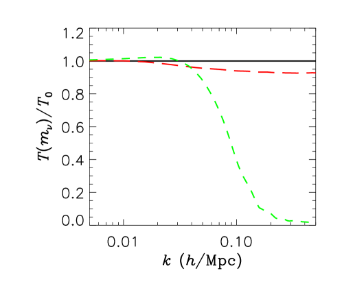
Figure 1: The transfer function $T(k,t=t_{0})$ for various different neutrino masses. The solid (black) line is for $m_{\nu}=0$, the long-dashed for $m_{\nu}=0.3$ eV, and the dashed for $m_{\nu}=1$ eV.

When measuring fluctuations it is customary to use the power spectrum, $P(k,\tau)$, defined as

$$P(k,\tau)=|\delta|^{2}(\tau).$$ (20)

The power spectrum can be decomposed into a primordial part, $P_{0}(k)$, and a transfer function $T(k,\tau)$,

$$P(k,\tau)=P_{0}(k)T(k,\tau).$$ (21)

The transfer function at a particular time is found by solving the Boltzmann equation for $\delta(\tau)$.

At scales much smaller than the free-streaming scale the present matter power spectrum is suppressed roughly by the factor [78]

$$\frac{\Delta P(k)}{P(k)}=\frac{\Delta T(k,\tau=\tau_{0})}{T(k,\tau=\tau_{0})}\simeq-8\frac{\Omega_{\nu}}{\Omega_{m}},$$ (22)

as long as $\Omega_{\nu}\ll\Omega_{m}$. The numerical factor 8 is derived from a numerical solution of the Boltzmann equation, but the general structure of the equation is simple to understand. At scales smaller than the free-streaming scale the neutrino perturbations are washed out completely, leaving only perturbations in the non-relativistic matter (CDM and baryons). Therefore the relative suppression of power is proportional to the ratio of neutrino energy density to the overall matter density. Clearly the above relation only applies when $\Omega_{\nu}\ll\Omega_{m}$, when $\Omega_{\nu}$ becomes dominant the spectrum suppression becomes exponential as in the pure hot dark matter model. This effect is shown for different neutrino masses in Fig. 1.

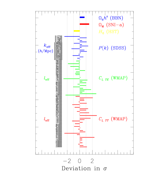
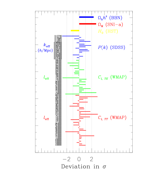
Figure 2: Deviation of the best fit models for $\sum m_{\nu}=0$ (left) and $\sum m_{\nu}=3$ eV (right). The CMB data shown are the WMAP binned data (http://lambda.gsfc.nasa.gov). The deviation is calculated as ”Deviation in $\sigma$” $=(A_{\rm model}-A_{\rm obs})/\sigma_{\rm obs}$.

The effect of massive neutrinos on structure formation only applies to the scales below the free-streaming length. For neutrinos with masses of several eV the free-streaming scale is smaller than the scales which can be probed using present CMB data and therefore the power spectrum suppression can be seen only in large scale structure data. On the other hand, neutrinos of sub-eV mass behave almost like a relativistic neutrino species for CMB considerations. The main effect of a small neutrino mass on the CMB is that it leads to an enhanced early ISW effect. The reason is that the ratio of radiation to matter at recombination becomes larger because a sub-eV neutrino is still relativistic or semi-relativistic at recombination. With the WMAP data alone it is very difficult to constrain the neutrino mass, and to achieve a constraint which is competitive with current experimental bounds it is necessary to include LSS data from 2dF or SDSS. When this is done the bound becomes very strong, somewhere in the range of 1 eV for the sum of neutrino masses, depending on assumptions about priors. In Table 2 the present upper bound on the neutrino mass from various analyses is quoted, as well as the assumptions going into the derivation.

Table 2: Various recent limits on the neutrino mass from cosmology and the data sets used in deriving them. 1: WMAP data, 2: Other CMB data, 3: 2dF data, 4: Constraint on $\sigma_{8}$ (different in $4^{a}$ and $4^{b}$), 5: SDSS data, 6: Constraint on $H_{0}$.

Ref.	Bound on $\sum m_{\nu}$	Data used
Spergel et al. (WMAP) [27]	0.69 eV	1,2,3,$4^{a}$,6
Hannestad [58]	1.01 eV	1,2,3,6
Allen, Smith and Bridle [83]	$0.56^{+0.3}_{-0.26}$ eV	1,2,3,$4^{b}$,6
Tegmark et al. (SDSS) [25]	1.8 eV	1,5
Barger et al. [89]	0.75 eV	1,2,3,5,6
Crotty, Lesgourgues and Pastor [81]	1.0 (0.6) eV	1,2,3,5 (6)

As can be gauged from this table, a fairly robust bound on the sum of neutrino masses is at present somewhere around 1.0 eV, depending somewhat on specific priors and data sets used.

It is also quite interesting to see what exactly provides this bound. It is often stated that the neutrino mass bound comes from large scale structure data, not from CMB because CMB probes larger scales. However, LSS data alone provides no limit on $\sum m_{\nu}$ because of degeneracies with other parameters (this is discussed in detail in Ref. [79]). On the other hand, WMAP in itself also does not provide a strong limit on the neutrino mass [25], because neutrino mass only has a limited effect on the scales probed by WMAP. Only the combination of the two types of data allows for a determination of $\sum m_{\nu}$ with any precision. Fig. 2 show deviation of the best fit models for $\sum m_{\nu}=0$ and $\sum m_{\nu}=3$ eV from WMAP and SDSS data. From this figure it is obvious that models with high neutrino mass are not ruled out by any single data point, but rather by a general decrease in how well the combined data fits. One fairly evident problem with the high neutrino mass model is that the shape of the large scale structure power spectrum becomes wrong. The model spectrum has too much power at intermediate scales and too little at small scales.

In the upper part of this figure the deviation of the best fit models from other cosmological data is shown. This data is not used in deriving the best fit models, and therefore the figure shows that the standard concordance model with $\sum m_{\nu}=0$ is not only a better fit to CMB and LSS data, but also more consistent with other cosmological data.

4.2.1 Combining measurements of $m_{\nu}$ and $N_{\nu}$.

The limits on neutrino masses discussed above apply only for neutrinos within the standard model, i.e. three light neutrinos with degenerate masses (if the sum is close to the upper bound). However, if there are additional neutrino species sharing the mass, or neutrinos have significant chemical potentials this bound is changed. Models with massive neutrinos have suppressed power at small scale, with suppression proportional to $\Omega_{\nu}/\Omega_{m}$. Adding relativistic energy further suppresses power at scales smaller than the horizon at matter-radiation equality. For the same matter density such a model would therefore be even more incompatible with data. However, if the matter density is increased together with $m_{\nu}$, and $N_{\nu}$, excellent fits to the data can be obtained. This effect is shown in Fig. 3.

Figure 3: Power spectra for $\Lambda$CDM models with $\Omega_{b}=0.05$, $\Omega=1$, $h=0.7$, $n_{s}=1$, and $N_{\nu,{\rm massive}}=1$ and a common large-scale normalization. The full line is for $\Omega_{\nu}=0$, $\Omega_{m}=0.25$, $N_{\nu}=3$, dashed is for $\Omega_{\nu}=0.05$, $\Omega_{m}=0.25$, $N_{\nu}=3$, dotted is for $\Omega_{\nu}=0.05$, $\Omega_{m}=0.25$, $N_{\nu}=8$, and long-dashed is for $\Omega_{\nu}=0.05$, $\Omega_{m}=0.35$, $N_{\nu}=8$ (from [80]).

The effect on likelihood contours for $(\Omega_{\nu},N_{\nu})$ can be seen in Fig. 4 which is for the case where $N_{\nu}$ species the total mass equally.

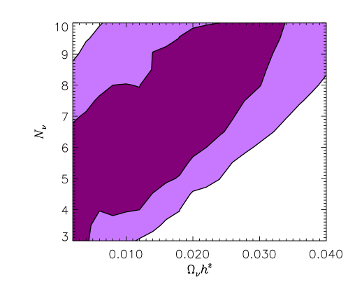
Figure 4: Likelihood contours (68% and 95%) for the case of $N_{\nu}$ neutrinos with equal masses, calculated from WMAP and 2dF data (from [80]).

A thorough discussion of these models can be found in Refs. [80, 81].

4.2.2 Future neutrino mass measurements

The present bound on the sum of neutrino masses is still much larger than the mass difference, $\Delta m_{23}\sim 0.05$ eV [90, 3], measured by atmospheric neutrino observatories and K2K . This means that if the sum of neutrino masses is anywhere close to saturating the bound then neutrino masses must the almost degenerate. The question is whether in the future it will be possible to measure masses which are of the order $\Delta m_{23}$, i.e. whether it can determined if neutrino masses are hierarchical.

By combining future CMB data from the Planck satellite with a galaxy survey like the SDSS it has been estimated that neutrino masses as low as about 0.1 eV can be detected [84, 85]. Another possibility is to use weak lensing of the CMB as a probe of neutrino mass. In this case it seems likely that a sensitivity below 0.1 eV can also be reached with CMB alone [92].

As noted in Ref. [85] the exact value of the sensitivity at this level depends both on whether the hierarchy is normal or inverted, and the exact value of the mass splittings.

4.3 Neutrino warm dark matter

While CDM is defined as consisting of non-interacting particles which have essentially no free-streaming on any astronomically relevant scale, and HDM is defined by consisting of particles which become non-relativistic around matter radiation equality or later, warm dark matter is an intermediate. One of the simplest production mechanisms for warm dark matter is active-sterile neutrino oscillations in the early universe [104, 105, 106, 107, 108].

One possible benefit of warm dark matter is that it does have some free-streaming so that structure formation is suppressed on very small scales. This has been proposed as an explanation for the apparent discrepancy between observations of galaxies and numerical CDM structure formation simulations. In general simulations produce galaxy halos which have very steep inner density profiles $\rho\propto r^{\alpha}$, where $\alpha\sim 1-1.5$, and numerous subhalos [93, 94]. Neither of these characteristics are seen in observations and the explanation for this discrepancy remains an open question. If dark matter is warm instead of cold, with a free-streaming scale comparable to the size of a typical galaxy subhalo then the amount of substructure is suppressed, and possibly the central density profile is also flattened [95, 96, 97, 98, 99, 100, 101] . In both cases the mass of the dark matter particle should be around 1 keV [109, 110], assuming that it is thermally produced in the early universe.

On the other hand, from measurements of the Lyman-$\alpha$ forest flux power spectrum it has been possible to reconstruct the matter power spectrum on relatively small scales at high redshift. This spectrum does not show any evidence for suppression at sub-galaxy scales and has been used to put a lower bound on the mass of warm dark matter particles of roughly 1.1 keV [103, 102]. An even more severe problem lies in the fact that star formation occurs relatively late in warm dark matter models because small scale structure is suppressed. This may be in conflict with the low-$l$ CMB temperature-polarization cross correlation measurement by WMAP which indicates very early reionization and therefore also early star formation. One recent investigation of this found warm dark matter to be inconsistent with WMAP for masses as high as 10 keV [95].

The case for warm dark matter therefore seems quite marginal, although at present it is not definitively ruled out by any observations.

4.4 Neutrinos as the source for high energy cosmic rays

Nucleons with energy above the threshold for photo-pion production on the CMB rapidly downscatter in energy, the mean free path being of order 20-30 Mpc. At the present CMB temperature of 2.7 K the threshold, known as the Greisen-Zatzepin-Kuzmin energy [118], is roughly $4\times 10^{19}$ GeV. On the other hand a significant number of particles with energies above the GZK energy have been observed. At present there is some controversy about the number of such particles observed between different experimental collaborations using different techniques. The HiRes [120] collaboration finds a decline in the number of events beyond the GZK energy which is in fact compatible with a cut-off. On the other hand the AGASA [119] collaboration finds that the spectrum is consistent with no cut-off, and even with a hardening of the spectrum at very high energies. Recent reviews of these issues can be found in Ref. [121].

Either these particles must come from relatively nearby sources or they are not nucleons (or nuclei) with standard model interactions. One explanation which has been proposed is the $Z$-burst scenario [111, 112, 113, 114, 115]. In this model, neutrino primaries with very high energy, $E\gg E_{\rm GZK}$, annihilate with neutrinos in the cosmic background to produce the observed protons. The cross section is significantly enhanced at $E_{\rm CM}=m_{Z}$, corresponding to a neutrino primary energy of $E\sim m_{Z}^{2}/2E_{\nu,0}\sim m_{Z}^{2}/2m_{\nu}$. If neutrino masses are hierarchical then the largest mass is of order $m_{\nu}\sim\Delta m_{\rm atm}\sim 0.05$ eV, meaning that $E_{\nu}\sim 10^{23}$ eV. If neutrinos are produced by pion decay in AGNs this must mean that particles of even higher energies are produced there.

On the other hand, if neutrinos have masses close to saturating the cosmological bound then the primary energy can be significantly lower.

Another requirement is that the neutrino annihilation must take place within the GZK sphere. This leads to a too low flux unless the rate is somehow enhanced. It has previously been proposed that this can be explained in models with significant neutrino chemical potential [116]. However, the present cosmological bounds on $\eta$ rule this out. If neutrinos are of eV mass then they do have significant clustering on GZK scales which can also enhance the rate by a factor of about 2. If ultra high energy cosmic rays are explained by the $Z$-burst this means that a mass bound on neutrinos can in principle be obtained. In Refs. [113, 114] it was estimated that if the annihilations are within the galactic halo it requires a neutrino mass of $m_{\nu}=2.34^{+1.29}_{-0.84}$ eV, and if the annihilation happens within the local supercluster the mass must be $m_{\nu}=0.26^{+0.20}_{-0.14}$ eV. The first case is already ruled out, but the second possibility might work. It has, however, also been shown that the values obtained in [113, 114] are strongly model dependent [117].

At present the feasibility of the $Z$-burst scenario remains an open question. One problem is that the annihilation process produces a background of low energy gamma rays which may be in conflict with EGRET observations, depending on the magnitude of the local neutrino density enhancement.

In any case the $Z$-burst scenario is also interesting from the possibility of getting an independent detection of the cosmological neutrino background if the needed very high fluxes of ultra-high energy neutrinos is measured in future detectors like Auger.

5 Neutrinos in the very early universe - Leptogenesis

A particularly attractive model for baryogenesis involves massive, right handed neutrinos, and is known as baryogenesis via leptogenesis [122]. The basic idea is that the masses of left handed Majorana neutrinos are generated from couplings to very massive, right handed neutrinos.

These massive, right handed states are unstable and because they are Majorana particles their decay violate lepton number. Futhermore the decays are out of equilibrium and can violate CP which means that all the Sakharov conditions for generating a net lepton number are present. This lepton number can then subsequently be transferred to the baryon sector via standard model interactions and account for the observed baryon number of the universe.

A particularly simple model for this is thermal leptogenesis where the right handed neutrinos are equilibrated at high temperatures directly via their interactions with the thermal plasma. In this case, the correct baryon number is produced only if the following conditions are fulfilled [123, 124, 125, 126, 127, 128]: a) Masses of the light neutrinos must be less than about 0.1-0.15 eV, and b) Masses of the right handed neutrinos must be larger than about $10^{8}$ GeV. The first condition is interesting because it provides a strong, albeit very model dependent, bound on the light neutrino masses. The second condition is interesting because it is so high that it might be in conflict with the upper bound on the reheating temperature in supersymmetric models. This bound arises from overproduction and subsequent decay of gravitinos and could probably be relaxed in models where the gravitino is the lightest supersymmetric particle.

Taken at face value the thermal leptogenesis constraint on light neutrino masses is the most restrictive cosmological limit known. However, it is not a constraint at the same level as experimental bounds, or even bounds from CMB and large scale structure. The derivation involves a chain of assumptions: a) Leptogenesis is the correct model of baryogenesis, b) leptogenesis is thermal, c) The heavy neutrino masses are hierarchical. If either of the first two assumptions are relaxed then there is essentially no mass bound from this argument. If the last assumption is relaxed then it has been shown in Ref. [128] that the mass bound on the left handed neutrinos can be relaxed by almost an order of magnitude.

With this in mind specific mass bounds on neutrino masses from thermal leptogenesis should be taken as both interesting and suggestive, but not as strict and generally applicable bounds.

6 Discussion

In the present paper I have discussed how cosmological observations can be used for probing fundamental properties of neutrinos which are not easily accessible in lab experiments. Particularly the measurement of absolute neutrino masses from CMB and large scale structure data has received significant attention over the past few years. In Table 3 I summarize neutrino mass bounds from cosmological observations and other astrophysical and experimental bounds.

Table 3: Summary table of cosmological neutrino mass limits. For completeness bounds from other sources, astrophysical and experimental, are also listed.

Method	Bound on $\sum m_{\nu}$	Data used
$\Omega_{\nu}h^{2}\,\hbox to0.0pt{\lower 3.5pt\hbox{$\mathchar 0\relax\sim$}\hss}\raise 1.0pt\hbox{$<$}\,0.15$	14 eV	$\Omega_{\nu}<\Omega_{m}$
CMB and LSS	0.7-1 eV	WMAP, 2dF, SDSS
SN1987A	$m_{\nu_{e}}<5-20$ eV $(\bar{\nu}_{e})$	SN1987A cooling curve [129, 130]
$\beta$-decay	$m_{\nu_{e}}<2.2$ eV $(\nu_{e})$	Mainz experiment [21]
$0\nu 2\beta$-decay	$m_{\nu,{\rm eff}}<0.35$ eV	Heidelberg-Moscow [131]
	0.1 eV $<m_{\nu,{\rm eff}}<$ 0.9 eV	Heidelberg-Moscow [22, 23]

Another cornerstone of neutrino cosmology is the measurement of the total energy density in non-electromagnetically interacting particles. For many years Big Bang nucleosynthesis was the only probe of relativistic energy density, but with the advent of precision CMB and LSS data it has been possible to complement the BBN measurement. At present the cosmic neutrino background is seen in both BBN, CMB and LSS data at high significance.

Finally, cosmology can also be used to probe the possibility of neutrino warm dark matter, which could be produced by active-sterile neutrino oscillations.

In the coming years the steady stream of new observational data will continue, and the cosmological bounds on neutrino will improve accordingly. For instance, it has been estimated that with data from the upcoming Planck satellite it could be possible to measure neutrino masses as low as 0.1 eV.

Certainly neutrino cosmology will continue to be a prospering field of research for the foreseeable future.

References

References

- [1] P. Aliani, V. Antonelli, M. Picariello and E. Torrente-Lujan, arXiv:hep-ph/0309156.
- [2] P. C. de Holanda and A. Y. Smirnov, arXiv:hep-ph/0309299.
- [3] M. Maltoni, T. Schwetz, M. A. Tortola and J. W. F. Valle, Phys. Rev. D 68, 113010 (2003) [arXiv:hep-ph/0309130].
- [4] V. A. Kostelecky and S. Samuel, Phys. Lett. B 318, 127 (1993).
- [5] G. M. Fuller, J. R. Primack and Y. Z. Qian, Phys. Rev. D 52, 1288 (1995) [arXiv:astro-ph/9502081].
- [6] D. O. Caldwell and R. N. Mohapatra, Phys. Lett. B 354, 371 (1995) [arXiv:hep-ph/9503316].
- [7] S. M. Bilenky, C. Giunti, C. W. Kim and S. T. Petcov, Phys. Rev. D 54, 4432 (1996) [arXiv:hep-ph/9604364].
- [8] S. F. King and N. N. Singh, Nucl. Phys. B 596, 81 (2001) [arXiv:hep-ph/0007243].
- [9] H. J. He, D. A. Dicus and J. N. Ng, arXiv:hep-ph/0203237.
- [10] A. Ioannisian and J. W. Valle, Phys. Lett. B 332, 93 (1994) [arXiv:hep-ph/9402333].
- [11] P. Bamert and C. P. Burgess, Phys. Lett. B 329, 289 (1994) [arXiv:hep-ph/9402229].
- [12] R. N. Mohapatra and S. Nussinov, Phys. Lett. B 346, 75 (1995) [arXiv:hep-ph/9411274].
- [13] H. Minakata and O. Yasuda, Phys. Rev. D 56, 1692 (1997) [arXiv:hep-ph/9609276].
- [14] F. Vissani, arXiv:hep-ph/9708483.
- [15] H. Minakata and O. Yasuda, Nucl. Phys. B 523, 597 (1998) [arXiv:hep-ph/9712291].
- [16] J. R. Ellis and S. Lola, Phys. Lett. B 458, 310 (1999) [arXiv:hep-ph/9904279].
- [17] J. A. Casas, J. R. Espinosa, A. Ibarra and I. Navarro, Nucl. Phys. B 556, 3 (1999) [arXiv:hep-ph/9904395].
- [18] J. A. Casas, J. R. Espinosa, A. Ibarra and I. Navarro, Nucl. Phys. B 569, 82 (2000) [arXiv:hep-ph/9905381].
- [19] E. Ma, J. Phys. G 25, L97 (1999) [arXiv:hep-ph/9907400].
- [20] R. Adhikari, E. Ma and G. Rajasekaran, Phys. Lett. B 486, 134 (2000) [arXiv:hep-ph/0004197].
- [21] C. Kraus et al. European Physical Journal C (2003), proceedings of the EPS 2003 - High Energy Physics (HEP) conference.
- [22] H. V. Klapdor-Kleingrothaus, A. Dietz, H. L. Harney and I. V. Krivosheina, Mod. Phys. Lett. A 16, 2409 (2001) [arXiv:hep-ph/0201231].
- [23] H. V. Klapdor-Kleingrothaus, I. V. Krivosheina, A. Dietz and O. Chkvorets, Phys. Lett. B 586, 198 (2004) [arXiv:hep-ph/0404088].
- [24] M. Tegmark et al. [SDSS Collaboration], arXiv:astro-ph/0310725.
- [25] M. Tegmark et al. [SDSS Collaboration], arXiv:astro-ph/0310723.
- [26] J. A. Peacock et al., Nature 410 (2001) 169 [astro-ph/0103143].
- [27] D. N. Spergel et al., Astrophys. J. Suppl. 148 (2003) 175 [astro-ph/0302209].
- [28] C. L. Bennett et al., Preliminary maps and basic results,” Astrophys. J. Suppl. 148 (2003) 1 [astro-ph/0302207].
- [29] A. Kogut et al., Astrophys. J. Suppl. 148 (2003) 161 [astro-ph/0302213].
- [30] G. Hinshaw et al., Astrophys. J. Suppl. 148 (2003) 135 [astro-ph/0302217].
- [31] L. Verde et al., Astrophys. J. Suppl. 148 (2003) 195 [astro-ph/0302218].
- [32] H. V. Peiris et al., Astrophys. J. Suppl. 148 (2003) 213 [astro-ph/0302225].
- [33] C. l. Kuo et al. [ACBAR collaboration], Astrophys. J. 600, 32 (2004) [arXiv:astro-ph/0212289].
- [34] X. Wang, M. Tegmark, B. Jain and M. Zaldarriaga, astro-ph/0212417.
- [35] W. L. Freedman et al., Astrophys. J. 553 (2001) 47 [astro-ph/0012376].
- [36] R. A. Knop et al., arXiv:astro-ph/0309368.
- [37] E. W. Kolb and M. S. Turner, “The Early Universe,”, Addison-Wesley (1990).
- [38] S. Hannestad and J. Madsen, Phys. Rev. D 52, 1764 (1995) [arXiv:astro-ph/9506015].
- [39] D. A. Dicus, E. W. Kolb, A. M. Gleeson, E. C. Sudarshan, V. L. Teplitz and M. S. Turner, Phys. Rev. D 26, 2694 (1982).
- [40] N. C. Rana and B. Mitra, Phys. Rev. D 44, 393 (1991).
- [41] M. A. Herrera and S. Hacyan, Astrophys. J. 336, 539 (1989).
- [42] A. D. Dolgov and M. Fukugita, Phys. Rev. D 46, 5378 (1992).
- [43] S. Dodelson and M. S. Turner, Phys. Rev. D 46, 3372 (1992).
- [44] B. D. Fields, S. Dodelson and M. S. Turner, Phys. Rev. D 47, 4309 (1993) [arXiv:astro-ph/9210007].
- [45] A. D. Dolgov, S. H. Hansen and D. V. Semikoz, Nucl. Phys. B 503, 426 (1997) [arXiv:hep-ph/9703315].
- [46] A. D. Dolgov, S. H. Hansen and D. V. Semikoz, Nucl. Phys. B 543, 269 (1999) [arXiv:hep-ph/9805467].
- [47] N. Y. Gnedin and O. Y. Gnedin, Astrophys. J. 509, 11 (1998).
- [48] S. Esposito, G. Miele, S. Pastor, M. Peloso and O. Pisanti, Nucl. Phys. B 590, 539 (2000) [arXiv:astro-ph/0005573].
- [49] G. Steigman, arXiv:astro-ph/0108148.
- [50] G. Mangano, G. Miele, S. Pastor and M. Peloso, arXiv:astro-ph/0111408.
- [51] S. Hannestad, Physical Review D 65, 083006 (2002).
- [52] V. Barger, J. P. Kneller, H. S. Lee, D. Marfatia and G. Steigman, Phys. Lett. B 566, 8 (2003) [arXiv:hep-ph/0305075].
- [53] A. Cuoco, F. Iocco, G. Mangano, G. Miele, O. Pisanti and P. D. Serpico, arXiv:astro-ph/0307213.
- [54] H. S. Kang and G. Steigman, Nucl. Phys. B 372, 494 (1992).
- [55] K. Kohri, M. Kawasaki and K. Sato, Astrophys. J. 490, 72 (1997) [arXiv:astro-ph/9612237].
- [56] M. Orito, T. Kajino, G. J. Mathews and Y. Wang, Phys. Rev. D 65, 123504 (2002) [arXiv:astro-ph/0203352].
- [57] K. Ichikawa and M. Kawasaki, Phys. Rev. D 67, 063510 (2003) [arXiv:astro-ph/0210600].
- [58] S. Hannestad, JCAP 0305 (2003) 004 [astro-ph/0303076].
- [59] P. Crotty, J. Lesgourgues and S. Pastor, Phys. Rev. D 67, 123005 (2003) [arXiv:astro-ph/0302337].
- [60] E. Pierpaoli, Mon. Not. Roy. Astron. Soc. 342, L63 (2003) [arXiv:astro-ph/0302465].
- [61] A. D. Dolgov, Phys. Rept. 370, 333 (2002) [arXiv:hep-ph/0202122].
- [62] C. Lunardini and A. Y. Smirnov, Phys. Rev. D 64, 073006 (2001) [arXiv:hep-ph/0012056].
- [63] S. Pastor, G. G. Raffelt and D. V. Semikoz, arXiv:hep-ph/0109035.
- [64] A. D. Dolgov, S. H. Hansen, S. Pastor, S. T. Petcov, G. G. Raffelt and D. V. Semikoz, Nucl. Phys. B 632, 363 (2002) [arXiv:hep-ph/0201287].
- [65] K. N. Abazajian, J. F. Beacom and N. F. Bell, Phys. Rev. D 66, 013008 (2002) [arXiv:astro-ph/0203442].
- [66] Y. Y. Wong, Phys. Rev. D 66, 025015 (2002) [arXiv:hep-ph/0203180].
- [67] M. Kawasaki, K. Kohri and N. Sugiyama, Phys. Rev. Lett. 82, 4168 (1999) [arXiv:astro-ph/9811437].
- [68] Phys. Rev. D 62, 023506 (2000) [arXiv:astro-ph/0002127].
- [69] G. F. Giudice, E. W. Kolb and A. Riotto, Phys. Rev. D 64, 023508 (2001) [arXiv:hep-ph/0005123].
- [70] G. F. Giudice, E. W. Kolb, A. Riotto, D. V. Semikoz and I. I. Tkachev, Phys. Rev. D 64, 043512 (2001) [arXiv:hep-ph/0012317].
- [71] S. Hannestad, arXiv:astro-ph/0403291.
- [72] S. S. Gershtein and Y. B. Zeldovich, JETP Lett. 4, 120 (1966) [Pisma Zh. Eksp. Teor. Fiz. 4, 174 (1966)].
- [73] R. Cowsik and J. McClelland, Phys. Rev. Lett. 29, 669 (1972).
- [74] S. Tremaine and J. E. Gunn, Phys. Rev. Lett. 42, 407 (1979).
- [75] J. Madsen, Phys. Rev. D 44, 999 (1991).
- [76] P. Salucci and A. Sinibaldi, Astron. Astrophys. 323, 1 (1997).
- [77] C. P. Ma and E. Bertschinger, Astrophys. J. 455, 7 (1995) [arXiv:astro-ph/9506072].
- [78] W. Hu, D. J. Eisenstein and M. Tegmark, Phys. Rev. Lett. 80 (1998) 5255 [astro-ph/9712057].
- [79] O. Elgaroy and O. Lahav, JCAP 0304 (2003) 004 [astro-ph/0303089].
- [80] S. Hannestad and G. Raffelt, arXiv:hep-ph/0312154.
- [81] P. Crotty, J. Lesgourgues and S. Pastor, arXiv:hep-ph/0402049.
- [82] S. Hannestad, Phys. Rev. D 66 (2002) 125011 [astro-ph/0205223].
- [83] S. W. Allen, R. W. Schmidt and S. L. Bridle, astro-ph/0306386.
- [84] S. Hannestad, Phys. Rev. D 67 (2003) 085017 [astro-ph/0211106].
- [85] J. Lesgourgues, S. Pastor and L. Perotto, arXiv:hep-ph/0403296.
- [86] K. N. Abazajian and S. Dodelson, Phys. Rev. Lett. 91 (2003) 041301 [astro-ph/0212216].
- [87] U. Seljak and M. Zaldarriaga, Astrophys. J. 469 (1996) 437 [astro-ph/9603033]. See also the CMBFAST website at http://cosmo.nyu.edu/matiasz/CMBFAST/cmbfast.html
- [88] S. Perlmutter et al. [Supernova Cosmology Project Collaboration], Astrophys. J. 517 (1999) 565 [astro-ph/9812133].
- [89] V. Barger, D. Marfatia and A. Tregre, arXiv:hep-ph/0312065.
- [90] G. L. Fogli, E. Lisi, A. Marrone and D. Montanino, Phys. Rev. D 67, 093006 (2003) [arXiv:hep-ph/0303064].
- [91] A. Bandyopadhyay, S. Choubey, S. Goswami, S. T. Petcov and D. P. Roy, Phys. Lett. B 583, 134 (2004) [arXiv:hep-ph/0309174].
- [92] M. Kaplinghat, L. Knox and Y. S. Song, Phys. Rev. Lett. 91, 241301 (2003) [arXiv:astro-ph/0303344].
- [93] S. Kazantzidis, L. Mayer, C. Mastropietro, J. Diemand, J. Stadel and B. Moore, arXiv:astro-ph/0312194.
- [94] S. Ghigna, B. Moore, F. Governato, G. Lake, T. Quinn and J. Stadel, Astrophys. J. 544, 616 (2000) [arXiv:astro-ph/9910166].
- [95] N. Yoshida, A. Sokasian, L. Hernquist and V. Springel, Astrophys. J. 591, L1 (2003) [arXiv:astro-ph/0303622].
- [96] Z. Haiman, R. Barkana and J. P. Ostriker, arXiv:astro-ph/0103050.
- [97] V. Avila-Reese, P. Colin, O. Valenzuela, E. D’Onghia and C. Firmani, arXiv:astro-ph/0010525.
- [98] P. Bode, J. P. Ostriker and N. Turok, Astrophys. J. 556, 93 (2001) [arXiv:astro-ph/0010389].
- [99] P. Colin, V. Avila-Reese and O. Valenzuela, Astrophys. J. 542, 622 (2000) [arXiv:astro-ph/0004115].
- [100] S. Hannestad and R. J. Scherrer, Phys. Rev. D 62, 043522 (2000) [arXiv:astro-ph/0003046].
- [101] J. Sommer-Larsen and A. Dolgov, arXiv:astro-ph/9912166.
- [102] S. Colombi, S. Dodelson and L. M. Widrow, Astrophys. J. 458, 1 (1996) [arXiv:astro-ph/9505029].
- [103] V. K. Narayanan, D. N. Spergel, R. Dave and C. P. Ma, arXiv:astro-ph/0005095.
- [104] S. H. Hansen, J. Lesgourgues, S. Pastor and J. Silk, Mon. Not. Roy. Astron. Soc. 333, 544 (2002) [arXiv:astro-ph/0106108].
- [105] K. Abazajian, G. M. Fuller and W. H. Tucker, Astrophys. J. 562, 593 (2001) [arXiv:astro-ph/0106002].
- [106] K. Abazajian, G. M. Fuller and M. Patel, Phys. Rev. D 64, 023501 (2001) [arXiv:astro-ph/0101524].
- [107] X. d. Shi and G. M. Fuller, Phys. Rev. Lett. 82, 2832 (1999) [arXiv:astro-ph/9810076].
- [108] S. Dodelson and L. M. Widrow, Phys. Rev. Lett. 72, 17 (1994) [arXiv:hep-ph/9303287].
- [109] C. J. Hogan and J. J. Dalcanton, Phys. Rev. D 62, 063511 (2000) [arXiv:astro-ph/0002330].
- [110] J. J. Dalcanton and C. J. Hogan, Astrophys. J. 561, 35 (2001) [arXiv:astro-ph/0004381].
- [111] T. J. Weiler, Phys. Rev. Lett. 49, 234 (1982).
- [112] T. J. Weiler, Astropart. Phys. 11, 303 (1999) [arXiv:hep-ph/9710431].
- [113] A. Ringwald, arXiv:hep-ph/0111112.
- [114] Z. Fodor, S. D. Katz and A. Ringwald, Phys. Rev. Lett. 88, 171101 (2002) [arXiv:hep-ph/0105064].
- [115] G. Gelmini and G. Varieschi, arXiv:hep-ph/0201273.
- [116] G. Gelmini and A. Kusenko, Phys. Rev. Lett. 82, 5202 (1999).
- [117] O. E. Kalashev, V. A. Kuzmin, D. V. Semikoz and G. Sigl, Phys. Rev. D 65, 103003 (2002) [arXiv:hep-ph/0112351].
- [118] K. Greisen, Phys. Rev. Lett. 16, 748 (1966); G. T. Zatsepin and V. A. Kuzmin, JETP Lett. 4, 78 (1966).
- [119] N. Hayashida et al., arXiv:astro-ph/0008102.
- [120] R. U. Abbasi et al. [The High Resolution Fly’s Eye Collaboration (HIRES)], arXiv:astro-ph/0404137.
- [121] G. Sigl, arXiv:astro-ph/0404074.
- [122] M. Fukugita and T. Yanagida, Phys. Lett. B 174, 45 (1986).
- [123] S. Davidson and A. Ibarra, hep-ph/0202239
- [124] K. Hamaguchi, H. Murayama and T. Yanagida, hep-ph/0109030
- [125] W. Buchmuller, P. di Bari and M. Pluemacher, Nucl. Phys. B 665, 445 (2003).
- [126] W. Buchmuller and M. Pluemacher, Phys. Rept. 320, 329 (1999).
- [127] G. F. Giudice et al., hep-ph/0310123.
- [128] T. Hambye et al., hep-ph/0312203
- [129] P. J. Kernan and L. M. Krauss, Nucl. Phys. B 437, 243 (1995) [arXiv:astro-ph/9410010].
- [130] T. J. Loredo and D. Q. Lamb, Phys. Rev. D 65, 063002 (2002) [arXiv:astro-ph/0107260].
- [131] H. V. Klapdor-Kleingrothaus et al., Eur. Phys. J. A 12, 147 (2001) [arXiv:hep-ph/0103062].