Constraining the string scale: from Planck to Weak and back again

Abstract

String and field theory ideas have greatly influenced each other since the so called second string revolution. We review this interrelation paying particular attention to its phenomenological implications. Our guiding principle is the radical shift in the way that we think about the fundamental scale, in particular the way in which string models have been able to accommodate values from the Planck $M_{\mathrm{Pl}}\sim 10^{18}$ GeV down to the electroweak scale $M_{EW}\sim$ TeV.

1 Vacuum degeneracy: vice or virtue?

There are two purposes to this article. The first is as an overview (for an experimental audience) of string theory developments in the past 8 years or so, since the so-called 2nd string revolution, concentrating on aspects that have to do with “phenomenology”. Many ideas that are now common, such as large extra dimensions, have arisen from string theory or at least been inspired by it. Conversely ideas couched purely in terms of for example extra dimensional field theory have often guided subsequent string theory developments. For the lay audience the resulting picture has become exceedingly obscure, and there is a clear need for some kind of overview. This article is an attempt to meet this need by focussing on one particular area where our ideas have radically changed in the past few years, namely what the fundamental scale of gravity, or string scale, ought to be. In the first half of the article therefore, we shall discuss how string models have consistently been able to accommodate successively lower string scales, until today it is possible to construct models that have fundamental scales of order a few TeV.

The second purpose of this article is to address the most immediate question that presents itself to people with a more phenomenological viewpoint, namely whether such low scale string models have anything to do with reality, i.e. do they have any repercussions for experiment? We shall argue that they indeed do and that flavour changing effects constrain the string scale to be higher than $10^{3}$ TeV thereby eliminating a whole tranche of low scale string models. A more optimistic phraseology would be to say that experiment is already probing string scales of order $10^{3}$ TeV. This indicates, we think, that string theory is finally becoming an honest theory, that is one that can be readily disproved by experiment.

A subsidiary purpose of this article, of interest to those concerned with extra dimensional field theories, is to show how most conceivable ideas that have been discussed in field theory terms can be constructed and tested in a stringy set-up. The obvious virtues of the latter are that questions that are difficult to address (e.g. divergences) or impossible to address (e.g. quantum effects) in extra dimensional field theory models, are usually resolved in string theory.

We begin with a discussion of how we used to estimate the fundamental scale of quantum-gravity. The familiar estimate is a dimensional one, based on measured constants of nature

$$\left.\begin{array}[]{l}G=6.673\times 10^{-11}m^{3}\operatorname{kg}^{-1}s^{-2}\\ h=1.055\times 10^{-34}Js\\ c=2.997\times 10^{8}ms^{-1}\end{array}\right\}\rightarrow L_{\operatorname{Pl}}=\sqrt{Gh/c^{3}}=1.61\times 10^{-33}\operatorname{cm}$$

The resulting Planck length ($\equiv M_{\operatorname{Pl}}=1.22\times 10^{19}\operatorname{GeV})$ is the scale at which we used to think quantum-gravity effects would first make themselves felt.

What can go wrong with this estimate? The crucial point, emphasized in Ref.[1], is that the energy scale at which we measure $G_{N}$ is vastly different from $M_{\operatorname{Pl}}$ itself. (This is possible because, alone among the forces, the effect on gravity of adding extra masses is always positive.) The implicit assumption is that in between the two scales there are no abnormally large parameters entering into the physics. In particular for this discussion, in theories which have extra dimensions that are much larger than the fundamental scale, the measured Newton’s constant can be much weaker than expected because the gravitational force is diluted by the extra volume. Indeed the naive relation is

$$G_{4}\sim V^{-1}_{D-4}G_{D}$$

where $V_{D-4}$ is the volume of whatever extra dimensions our theory happens to have. (Note that we will for simplicity only consider flat extra dimensions.) If for example we have a fundamental scale of $M_{s}\sim 1\operatorname{TeV}$ then $V_{D-4}\sim 10^{32}$ (in fundamental lengths) gives the required enhancement factor of $10^{16}$ to the Planck mass. If $D=10$ then we would require the extra dimensions to be of order $\operatorname{few}\times 10^{5}\operatorname{TeV}^{-1}.$

On the other hand gauge forces cannot consistently be allowed to feel the same extra dimensional volumes. This is because gauge couplings are dimensionless so that the extra volume would just lead to either nonperturbatively large or immeasurably small couplings. (They could feel some large volumes however, in which case there is some rescaling required and the relationships become a little more complicated but similar.)

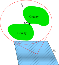
Figure 1: Brane world picture with 4 large flat dimensions represented as a plane and extra small dimensions determining the different scales of nature.

The generic picture for significantly changing the scale of quantum gravity is therefore as shown in Figure 1. The large flat 4 dimensional space in which we apparently live is shown as the flat plane. Blowing up any portion of it reveals an internal space that determines all of the physics (supersymmetry, particle content and so on). The fundamental scale can be much lower than the Planck scale if gravity feels a large internal volume (denoted by green blobs), with the Standard Model (SM) fields being confined to some restricted subvolume.

This type of set up is a natural possibility in string theory with its 6 extra dimensions, but large extra dimensions are a reasonable thing to consider only because of a feature of string theory that we used to regard as a problem, namely the vacuum degeneracy problem. To summarize, the problem is that string theory gives no hints as to the shape or size of the compactified vacua, or even the number of compactified dimensions. So for example we have no explanation as to why there are 4 large flat dimensions. More specifically this can be stated as follows. The size and shape of a particular compactification manifold can be specified by various parameters (for example the various radii), known collectively as moduli. Choosing a particular compactification radius corresponds to fixing these parameters. Since they determine the 4 dimensional physics they should of course be the same (i.e. Figure 1 should look the same) at every point in $M_{4}$. However these parameters correspond to the VEVs of fields in the spectrum that are left over from the higher dimensional metric. These fields turn out to be massless, and indeed their potential is completely flat to all orders in perturbation theory. (In terms of Figure 1, if for example we perturb the compactification manifold at a particular point in $M_{4}$ then all the neighbouring manifolds are perturbed and so on, and a signal radiates out at the speed of light in $M_{4}$; these are the massless particles.) In addition we are at liberty to set the compactification to be as large as we like, with the hope that our preferred choice will at some stage be explained by a non-perturbative contribution to the moduli potential. So when it comes to lowering the fundamental scale, the vacuum degeneracy problem is seen as a virtue.

2 The road to $M_{s}=M_{W}$

We now turn to how this idea has been realized in stringy set-ups. For this we first need a “road-map” of string theory in order to orient ourselves; we begin with the canonical layout of 10 dimensional string theory plus supergravity shown in Figure 2.

Figure 2: M-theory road map

Five of the labelled points represent the various perturbative regimes (i.e. different kinds of string theory) that can be written down in 10 dimensions. These are Heterotic, and type IIA/B, all of which are theories of closed strings, and type I which is an $\operatorname{SO}(32)$ theory of open strings. In addition the diagram includes a sixth point representing 11D supergravity. The triumph of the 2nd string revolution was to demonstrate that by applying successive duality transformations it is possible to get from any of the 6 perturbative points on this diagram to any other. The conjecture is therefore that the perturbative theories are simply limits of some nonperturbative underlying theory which encompasses the whole of this diagram, for which the search continues. In the meantime one can consider the phenomenological possibilities for the 6 theories where we can do perturbation theory.

In the following sections our phenomenological discussion will take us to all the different corners of this road map. The itinerary is determined by the value of the string scale in the different models, starting with the most conservative case of a string scale of the order of the Planck mass in weakly coupled heterotic models down to GUT string scale (strongly coupled heterotic), intermediate scale models (type I and II models) and finally discussing the radical idea of a TeV string scale (in non-supersymmetric models with D-branes intersecting at non-trivial angles).

3 From $M_{s}\sim M_{\mathrm{Pl}}$ to $M_{s}\sim M_{\mathrm{GUT}}$: weakly and strongly coupled heterotic models

At first sight (i.e. perturbatively) only the Heterotic models seem to be of much use for model building. This is because they alone contain both quantum gravity and gauge fields. Gravity, being a spin 2 field, requires closed strings which rules out type I. However the type II models are also ruled out because they only contain gravity multiplets and no gauge fields. Heterotic theories are also closed strings, but they are a curious combination of supersymmetric and bosonic string theories. The former can exist in 10 dimensions whereas the latter require 26. The 16 additional internal degrees of freedom in the bosonic half then become gauge degrees of freedom in the effective theory; hence the gauge groups must have rank 16 and indeed anomaly cancellation restricts them still further to be $E_{8}\times E_{8}$ or $\operatorname{SO}(32)$ (the latter turns out to be dual to the SO(32) of the type I models).

Model building in heterotic strings concentrated on the $E_{8}\times E_{8}$ gauge group. In order to get N=1 supersymmetry in 4 dimensions, the compactification manifold $K_{6}$ has to be of a certain type (Calabi-Yau) and consistency requires a breaking of the gauge group by the compactification. One attractive route of gauge breaking is then

$$E_{8}\times E^{\prime}_{8}\longrightarrow\operatorname{SU}(3)\times E_{6}\times E_{8}^{\prime}\longrightarrow \operatorname{MSSM}\times\operatorname{hidden}$$

This route arose from a particularly simple way of satisfying the various consistency conditions that compactification imposes, which became known as the “standard embedding”. The first $E_{6}$ factor is a potential Grand Unified group whereas the second $E^{\prime}_{8}$ factor forms a hidden sector group. The latter is a potential source of supersymmetry breaking by for example the condensing of the gaugino of some hidden sector group at a high mass scale (much like the condensation that takes place in QCD leading to a $\Lambda_{\operatorname{QCD}}$ breaking).

Let us now turn to the question of the fundamental scale. As we have said, in heterotic models, all degrees of freedom in the perturbative model are the result of excitations of closed strings. All closed strings can travel everywhere in the compact space and so both gauge and gravity degrees of freedom necessarily feel the same compact volume, $V_{6}$ say. The Planck scale and the gauge couplings can then be simply computed from the dimensional reduction of the 10-dimensional theory. In terms of the string scale, $M_{s}$, and the heterotic string coupling, $\lambda_{H}$, they read

$$M^{2}_{\mathrm{Pl}}\sim\frac{V_{6}}{\lambda_{H}^{2}}M_{s}^{8},$$ (1)

and

$$\alpha_{YM}\sim\frac{\lambda_{H}^{2}}{V_{6}M_{s}^{6}}.$$ (2)

These expressions, together with the experimental fact that $\alpha_{YM}\lesssim 1$, imply, in the case that the heterotic string remains weakly coupled (i.e. $\lambda_{H}\lesssim 1$), the following relations between the compactification, string and Planck scales

$$M_{s}\sim M_{Pl}\sim V_{6}^{1/6}.$$ (3)

Things are less simple in the strongly coupled limit. The strongly coupled $E_{8}\times E_{8}$ heterotic is only tractable thanks to the fact that, as Horava and Witten showed [2], it is described by 11-dimensional supergravity compactified on an $S^{1}/Z_{2}$ orbifold. Based on anomaly cancellation arguments they argued that an $E_{8}$ gauge group lives on each of the two 10-dimensional orbifold fixed planes whereas gravity lives in the 11-dimensional bulk as sketched in Fig. 3. In the case of strong coupling, the radius of the orbifold $R_{11}$ is larger than the compactification scale of the 6 extra dimensions. It is therefore possible to consider the compactification of this theory down to 4 dimensions in two steps, with an intermediate 5-dimensional model compactified on an orbifold.

Figure 3: Horava-Witten construction for the strong coupling limit of the $E_{8}\times E_{8}$ heterotic string. The green planes represent the 10-dimensional boundaries of the orbifold $S^{1}/Z_{2}$ where each $E_{8}$ factor lives, 11-dimensional supergravity propagates in the bulk.

The 11-dimensional action takes the form

$$S=\frac{1}{2\kappa_{11}^{2}}\int\mathrm{d}^{11}x\,\sqrt{g}R-\sum_{i}\frac{3^{1/3}}{4\pi(2\pi\kappa_{11}^{2})^{2/3}}\int\mathrm{d}^{10}x\,\sqrt{g}\mathrm{Tr}F_{i}^{2}+\ldots,$$ (4)

where $\kappa_{11}$ is the 11-dimensional gravitational constant and $i$ runs over the two 10-dimensional fixed planes where the two $E_{8}$ groups live. Compactifying down to five dimensions (with a compact volume $V_{6}$) and then to four dimensions we can write the fundamental 11-dimensional constant, $M_{11}=2\pi(4\pi\kappa_{11}^{2})^{-1/9}$ and the radius of the 11-th dimension, $R_{11}$, in terms of 4-dimensional quantities,

$$M_{11}=(2\alpha_{GUT}V_{6})^{-1/6},\quad R_{11}^{2}=\left(\frac{\alpha_{GUT}}{2}\right)^{3}V_{6}M_{\mathrm{Pl}}^{4}.$$ (5)

It is now possible to have

$$M_{11}\sim V_{6}^{-1/6}\sim M_{\mathrm{GUT}}\sim 10^{16}\mbox{ GeV},$$ (6)

and therefore $R_{11}^{-1}\sim 10^{13}-10^{15}$ GeV.

Thus we have seen how the heterotic string can accommodate a fundamental scale of the order of the Planck mass in the weak coupling limit, or GUT scale in the strong coupling limit. In the following sections we shall see how the existence of D-branes in type I and II theories allows an even greater reduction in the fundamental scale.

4 Intermediate models

The arrival of the large extra dimension idea stimulated interest in the other variants of string theory as model building tools. In particular attention turned to the type I and type II theories which have in their nonperturbative spectrum objects known as Dirichlet branes [3, 4]. These can be built like monopoles from the effective field theory, and are membrane-like and fully dynamical, with a typical surface tension and a width of order the fundamental scale. They have $p$ dimensions on their world volume where $p=1,3,5,7,9$ for type IIB, $1,5,9$ for type I and $0,2,4,6,8$ for type IIA. The interesting feature of D-branes from a model builder’s point of view is that open strings can end on them and this can generate gauge groups in the following way. Associated with an open string end point is an index, the Chan-Paton index. If there are a few branes together, the index simply labels the branes to which the open string is attached. If we consider two branes for example, the endpoints can be attached in one of 4 ways as in Figure 4.

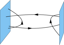
Figure 4: D-brane realization of a U(2) gauge group.

What do we see when we observe this from 4 dimensions? Remember that from the 4 dimensional point of view we need to arrange things such that the compactified space is the same everywhere. In particular the brane must be lying in the large $M_{4}$ space that we observe in order for the open string to be able to travel along it (otherwise it would be stuck at a single point in $M_{4}$. So the branes must have $p\geq 3$. (If $p=3$ the branes appear as points in the compactified space.) Given this, the open strings may freely propagate in $M_{4}$ but have 4 internal degrees of freedom corresponding to the adjoint of U(2). It also turns out that the strings have to have an excitation from the brane volume giving them a Lorentz (gauge boson) or internal (matter field) index. Finally a remarkable feature of D-branes is that they break only half the supersymmetry. Thus the original theory which has $N=8$ supersymmetry in 4 dimensions (if the compactified space is toroidal) ends up being $N=4$. We thus end up with an $N=4$ theory with $U(2)$ gauge group. In order to reach a more phenomenogically interesting $N=1$ configuration, the compactified space $K_{6}$ can be chosen in such a way that the supersymmetry is already partially broken before the D-branes are added. A type of compactification which is particularly easy to work with are orbifolds - spaces with curvature singularities at fixed points of the orbifolding (like the corners on cushions).

Before we start throwing branes together at random, we need to take care of some consistency conditions. The most important of these for D-branes are the Ramond-Ramond tadpole conditions. Every D-brane has a “Ramond-Ramond” (RR) charge, and couples to Ramond-Ramond fields that exist in the closed string spectrum (that is they are closed string excitations that are present in the type I or type II theory even before the D-branes are added in). Since these are closed string states they do not care about the presence or otherwise of the D-branes. In a toroidal compactification they propagate throughout the entire compactified volume. Curvature singularities, for example when the compactified space is an orbifold, introduce a second type of “twisted” RR field that is confined to the fixed points. The RR fields behave rather like gravitons and dilatons and form part of the gravitational spectrum. However they differ in the respect that flux lines of Ramond-Ramond fields must be absorbed in a compact space otherwise the theory is rendered entirely inconsistent. One has to be careful therefore to choose the arrangements of D-branes such that the flux lines are all absorbed. Once this requirement is satisfied, other requirements such as anomaly cancellation are usually satisfied as well.

These requirements led to an approach to model building which became known as “bottom-up” [5]. Consider what are the important features of any model from the point of view of phenomenology. The leading factors are those things that have to do with the gauge groups, particle content, number of generations and so on. Secondary factors are things that have to do with supersymmetry breaking, the cosmological constant etc. The latter are things whose eventual properties are intertwined with gravity. As such their influence on phenomenology is less important. In a large extra dimension set-up, the correspondence with the configuration in the compactified space is rather direct. The primary factors have to do with the local arrangements of D-branes around, for example, some orbifold fixed point, whereas the secondary factors are all associated with objects far away in the bulk of the compactified space. For example a “hidden” sector can be included consisting of a collection of branes at some other fixed point far away in the compactified space. The communication to the visible sector then has to be through the bulk, and will get the same volume suppression as that felt by gravity. This is shown schematically in Figure 5. The points represent for example D3 branes localized at some point in the compactified space with twisted RR flux cancelled locally. These are chosen in such a way that the visible sector is the MSSM. Gravity and the untwisted RR fields live in the bulk of the compactified space. These details and in particular the details of untwisted RR flux cancellation are less well determined.

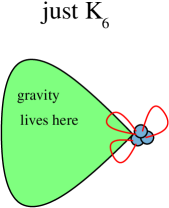
Figure 5: Schematic picture of the bottom-up approach. The small blue points represent the local configuration of D-branes leading to the MSSM whereas the large green blob represent the global structure, less important from a phenomenological viewpoint.

The bottom-up approach begins therefore by focussing on the local MSSM configuration. We assume an intermediate fundamental scale of

$$M_{I}\sim\sqrt{M_{W}M_{Pl}}\sim 10^{11}\,GeV.$$ (7)

This scale is familiar from the hidden sector supersymmetry breaking communicated by gravity and had been suggested earlier on more general grounds to do with supersymmetry breaking and mediation by gravity. First a set of D-branes is included at some fixed point of $K_{6}$ with all the necessary elements to make up the standard model gauge group and leave $N=1$ supersymmetry in the visible sector. This can for example be a set of D3-branes lying on top of each other at a single point in $K_{6}$, but with their world volumes filling the whole of $M_{4}$ (as of course we require if the open strings on their world volumes are able to travel anywhere in $M_{4}$). We then need to satisfy the requirements of local RR-tadpole cancellation. That is we need to add in additional branes (D7 branes for example) such that the “twisted” RR-tadpoles cancel but locally supersymmetry is preserved. This puts a constraint on the angles at which the branes can interesect (for example that the D7 branes intersect at right angles). This arrangement takes care of the local consistency conditions, however one should also take care of the global RR-tadpoles and make sure those fluxes cancel as well. This however can be done by adding other D-branes and anti-D branes elsewhere in the bulk or may be done in some other way. From the point of view of 4D phenomenology therefore, the particular way in which the global tadpoles are cancelled affects only the hidden sector, and consequently the soft supersymmetry breaking and cosmological constant. A consistent set-up is shown schematically in Figure 6. This figure shows the global RR flux being absorbed by anti-branes, but the set-up can be entirely different away from the visible sector without affecting the MSSM set-up directly.

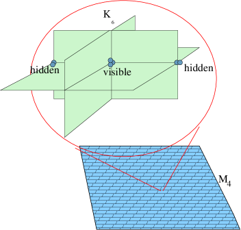
Figure 6: Set-up for the bottom up approach. The visible sector consists of 3-branes at a fixed point in $K_{6}$. D7 branes have to be included passing through this fixed point to cancel local RR-tadpoles. Global absence of tadpoles requires additional branes and/or anti-branes in the bulk, or possibly something else entirely.

The reason for the particular choice of the intermediate scale can now be made clear. The additional ingredients required to ensure global tadpole cancellation generally break supersymmetry. Since it is only the global configuration that breaks supersymmetry, the net effect is the same as hidden sector supersymmetry breaking communicated by gravity and we must choose the fundamental scale accordingly. In other words, the volume of the bulk can be responsible for the large Planck scale and the dilution of supersymmetry breaking effects only if $M_{s}\sim M_{I}$. The precise dependences on volumes can be derived from the reduction of the effective 10 dimensional type I action to 4 dimensions [13]. We begin with the Planck mass relation to the total compact volume

$$V_{K_{6}}=\lambda_{I}^{2}\frac{M_{P}^{2}}{M_{s}^{2}},$$ (8)

where $\lambda_{I}$ is the string coupling. To get an idea of what this has to be, we can look at the effective gauge coupling $\alpha_{p}$ on a $p$-dimensional brane. The gauge interactions are proportional to the string coupling but are diluted by the volume of the branes in the compactified space, $V_{p-3}$, since the gauge bosons are free to roam anywhere in this volume. Hence

$$\alpha_{p}\sim\frac{\lambda_{I}}{V_{p-3}}.$$ (9)

Substituting Eq. (9) into Eq. (8) gives us

$$\alpha_{p}M_{P}^{2}=M_{s}^{2}\frac{V_{9-p}}{V_{p-3}},$$ (10)

where $V_{9-p}$ is the co-volume (i.e. the volume orthogonal to the $p$ brane). Any process we care to calculate that breaks supersymmetry, such as a contribution to the scalar mass-squareds communicated via closed string modes from an anti-brane, feels the same volume dependence

$$m_{SUSY}^{2}\sim M_{s}^{2}\frac{V_{p-3}}{V_{9-p}}.$$ (11)

The dilution due to the co-volume $V_{9-p}$ is obvious. The $V_{p-3}$ enhancement factor arises from the sum over Kaluza-Klein (momentum) modes in the brane volume and is essentially the same factor as arising that arising in $1/\alpha_{p}$. Essentially this is like a phase space factor. (As a rule-of-thumb, one can use the fact that if we invert a radius, $R_{i}\rightarrow 1/R_{i}$, we also turn that dimension from a brane dimension into a dimension orthogonal to the brane or vice-versa, and also change the dimensionality of the brane, $p\rightarrow p\pm 1$. Hence the volumes must appear as the ratio of brane volume to co-volume, $V_{p-3}/V_{9-p}$.) There is no $1/\lambda_{I}$ contribution as there is in the tree level Yang-Mills terms (hence the equation for $\alpha_{p}$) because the diagrams that contribute to $M_{SUSY}$ are one-loop and $\lambda_{I}$ acts like a loop expansion parameter.

Now, for reasonable phenomenology we would like $M_{SUSY}\sim M_{W}$ so that from the above, and assuming that we have $\alpha_{p}\sim 1$ we need

$$M_{s}^{2}\sim M_{W}M_{P}$$

as expected, and consequently a volume ratio

$$\frac{V_{p-3}}{V_{9-p}}\sim\frac{M_{W}}{M_{P}}$$ (12)

The beauty of the bottom-up approach is that is allows us to disregard those parts of the construction that are not vital to phenomenology. For example there is a question of global validity of these models due to the fact that there are uncancelled tadpoles of another kind, namely NS-NS tadpoles. These however can be absorbed dynamically by adjusting the background (i.e. $K_{6}$) and their presence does not automatically render the theory inconsistent [7]. Although this effect may make the theory intractible on a global scale, it may still be a reasonable approximation to assume a nice (tractable) flat or orbifold background near the visible sector branes, where we can still calculate, for example, interactions.

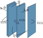
Figure 7: Local arrangement of states on D3-branes leading to the MSSM.

Let us turn briefly to the local arrangement of branes that yields the visible sector particle content and gauge group. This is often represented as in Figure 7. The Figure shows the arrangement of $D3$ branes at a particular fixed point in $K_{6}$. The branes are extended in $M_{4}$ and fixed in $K_{6}$ so that two of the dimensions shown are in $M_{4}$ and the dimension orthogonal to the branes should be in $K_{6}$. In addition the branes are on top of each other. (Any separation of branes translates into a mass for the relevant states due to the stretching energy.) There are three stacks of branes corresponding to a gauge group $U(3)\times U(2)\times U(1)$. The gauge states are those strings with ends attached on a single stack of branes. The matter states correspond to strings stretched between different stacks of branes and consequently appear (in this simple example) in the bifundamental. Thus we can identify strings stretched between the $U(3)$ and $U(2)$ stacks with left handed quarks, $Q_{L}$, between the $U(2)$ and $U(1)$ branes with left handed leptons and higgses, and between the $U(3)$ and $U(1)$ branes with right handed quarks. The gauge groups contain too many $U(1)$ factors, and the final reduction down to a single $U(1)_{Y}$ of hypercharge comes about because there is only one linear combination of $U(1)^{\prime}s$ that is anomaly free. Of course string theory is a consistent theory, and there should be no anomalies at all. But the way in which string theory cancels the anomalies makes the naively anomalous $U(1)^{\prime}s$ massive, and one expects that the anomalous combinations will be broken. Remarkably the states turn out to have the hypercharge assignments of the SM.

The bottom up approach has a number of advantages, many of which were outlined in Refs.[5, 8]. For example the prediction of an intermediate fundamental scale is interesting for a number of reasons. It is a natural realization of hidden sector supersymmetry breaking communicated by gravity. The model provides axions with just the right Peccei-Quinn scale to allow an axion solution to the string CP problem. In addition the see-saw mechanism for neutrino masses is consistent with a fundamental intermediate scale, and so on. One of the disadvantages of the bottom-up approach is that, by its very nature it is difficult to make concrete predictions of phenomenological implications. This is because the approach begins with a visible sector that resembles the MSSM and, by construction, aspects such as supersymmetry breaking have to do with the global configuration over which we assume very little control.

What then can be said about the emergent phenomenology? In the next subsections we will pick out a couple of areas that are currently exercising us, where the bottom-up approach can make generic predictions. The first concerns a little considered possibility in models that have several $U(1)$ factors, namely millicharged particles. The second related area has to do with the generic properties of supersymmetry breaking. At the end of this section we shall summarize where other progress has been made on this question.

4.1 Kinetic Mixing and Millicharged particles

Millicharged particles are a possibility in any theory that has a number of $U(1)^{\prime}s$, as string theories with stacks of D-branes generally do. The phenomenon that gives rise to this effect is known as Kinetic Mixing. Consider for example a field theory that has, in addition to some visible $U(1)_{a}$, a $U(1)_{b}$ factor in the hidden sector. Kinetic Mixing happens when the hidden $U(1)_{b}$ couples to the visible $U(1)_{a}$ through the diagram in Figure 8. The fields in the loop correspond to heavy states that do not appear in the low energy theory.

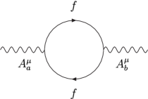
Figure 8: Contributions to Kinetic Mixing in field theory.

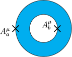
Figure 9: Contributions to Kinetic Mixing in string theory

This diagram, proportional to $Tr(Q_{a}Q_{b})$ , results in a Lagrangian of the form [9]

$$\mathcal{L}_{YM}=-\frac{1}{4}F_{a}^{\mu\nu}F_{a\mu\nu}-\frac{1}{4}F_{b}^{\mu\nu}F_{b\mu\nu}+\frac{\chi}{2}F_{a}^{\mu\nu}F_{b\mu\nu}$$ (13)

The most immediate consequences of this type of mixing were first studied by Holdom [9]. On diagonalizing the Yang-Mills lagrangian, one finds that the hidden sector fields charged only under $U(1)_{b}$ pick up a small charge of order $\chi$ under the visible sector $U(1)$. The bounds on such particles are very severe, especially if they are massless. In fact if $m_{hidden}<m_{e}$ there is a constraint of $\chi<10^{-15}$ coming from astrophysical bounds (specifically plasmon decay in Red Giants). Direct but much weaker experimental bounds of $\chi<10^{-4}$ are found from orthopositronium decay as well as a number of other accelerator and astrophysical sources [10].

This phenomenon generally arises in the intermediate models [11] because they include a hidden sector of anti D-branes in the bulk. Anti-branes and branes couple by exchanging closed string modes through the bulk. However a closed string exchange (which resembles a cylinder) can also be interpreted as an open string stretched between brane and anti-brane going in a loop as shown in Figure 9. The modes in the loop are heavy because they have a stretching energy proportional to their length (i.e. the distance between brane and anti-brane since they are stretched between them). Importantly the presence of anti-branes breaks supersymmetry. Therefore the one loop diagrams do not cancel (as they would in a supersymmetric configuration with just parallel branes for example), and there is a residual contribution to kinetic mixing and hence $\chi$.

Going back to the closed string exchange picture, it is (almost) obvious that the diagrams receive the same sort of volume suppression as the gravitational diagrams that lead to a large $M_{P}$. That is, the coupling $\chi$ is diluted by co-volume $V_{9-p}$ (i.e. the volume orthogonal to the D-branes) and enhanced by the brane volume $V_{p-3}$. However the normal Yang-Mills couplings are enhanced by the same $V_{p-3}$ factor since the gauge bosons travel the entire volume of the brane (indeed this is where Eq. (9) comes from). The suppression of the Kinetic Mixing term relative to the normal Yang Mills terms is therefore suppressed only by the co-volume but has an extra $\lambda_{I}$ factor because it is one-loop. Using the expression for $\alpha_{p}$ we can therefore write

$$\chi\sim Tr(Q_{a}Q_{b})\frac{\alpha_{p}V_{p-3}}{V_{9-p}}.$$ (14)

Comparing this to Eq. (12) we find

$$\chi\sim\alpha_{p}Tr(Q_{a}Q_{b})\frac{M_{W}}{M_{P}}.$$

Thus independently of $p$ this crude estimate gives the expected value of $\chi$ to be just below the bounds extracted from astrophysical considerations. However there are a number of factors that we have glossed over here for simplicity, and the situation can be slightly more complicated due to uncancelled NS-NS tadpoles, extremely non-degenerate extra dimensions and so on. One of the most important factors is that the volume dependence of $\chi$ does not quite go as the co-volume. Indeed if the radius of the co-volume is $R$ then the supersymmetry breaking mass-squared depend on $1/V_{9-p}\sim R^{p-9}$ whereas $\chi\sim R^{p-7}$ which merely reflects the fact that the potential is just that of gravitational attraction (e.g. in D space-time dimensions instead of 10 we have $R^{p-D-3}$ and get the familiar $1/R$ if we have particles/D0-branes in $D=4$.). The end result will be a more complicated dependence on $p$ and an enhanced millicharged particle effect with some cases being ruled out. For further details the reader is directed to Ref. [11].

4.2 Kinetic mixing and SUSY breaking

The consequences of $\chi\sim M_{W}/M_{P}$ are extremely interesting for supersymmetry breaking and it is to this that we now turn. Before we consider the specifics of kinetic mixing in detail we should mention some of the problems of supersymmetry breaking in generic models that we would like to be able to solve. One of the most enduring problems arises from possible flavour non-universality in the supersymmetry breaking terms. This leads to large violations of flavour from diagrams such as those in Figure 10 and large EDM contributions such as those in Figure 11.

Figure 10: Supersymmetry breaking contribution to $\Delta M_{K}$

Figure 11: Supersymmetry breaking contribution to $d-$EDM

In the former example, the flavour changing is driven by generational mass differences, $m_{\tilde{s}}^{2}-m_{\tilde{d}}^{2}$. In the second example, even though it is CP violating and flavour conserving, large contributions come from non-universal $A$-terms in the lagrangian once the fermions are rotated to their mass basis. These problems are known collectively as the supersymmetric flavour and CP problems. In the bottom-up configuration it is very difficult to say anything general about them. However one can identify new possibilities for solving them.

This is where Kinetic Mixing can play and important role. Dienes et al pointed out that Kinetic Mixing can contribute significantly and even dominantly to supersymmetry-breaking mediation [12]. This results in additional contributions to the scalar mass-squared terms proportional to their hypercharge (assuming the visible sector group is $U(1)_{Y}$, otherwise whatever the charge under $U(1)_{a}$ is) as follows. The supersymmetry breaking in the hidden sector is assumed to be maximal, and one expects a non-zero VEV for the D-terms of the hidden $U(1)_{b}$ of order

$$\langle D_{b}\rangle\sim M_{s}^{2}.$$ (15)

Upon kinetic mixing, the fields in the visible sector see this VEV through their $U(1)_{b}$ millicharges. That is the scalars pick up effective mass-squareds order

$$\tilde{m}^{2}\sim Q_{a}\chi M_{s}^{2}.$$ (16)

The interesting feature of the kinetic mixing in intermediate models is that it gives

$$\tilde{m}^{2}\sim Q_{a}\chi M_{I}^{2}\sim Q_{a}M_{W}^{2}.$$

The volume factors required to produce the large Planck mass therefore match those required to suppress $\chi$ to be $M_{W}/M_{P}$. Furthermore the mass-squared terms are proportional to hypercharge and is therefore generation independent. What we have found in intermediate models therefore is a source of degenerate mass-squareds of order $M_{W}^{2}$ that can be used to solve or at least ameliorate some of the problems of generic supersymmetric models. As pointed out by in ref[12], Kinetic Mixing to hypercharge cannot be the only source of mediation, as some of the mass-squareds would have to be negative however the problem should be reduced. Alternatively one could invoke a second $U(1)_{a}$ group in the visible sector that provides additional positive mass-squared contributions.

It is interesting to contrast the Kinetic Mixing here with that in Ref.[12]. In a model with a string scale of say $M_{s}\sim M_{GUT}$, including $\chi\sim M_{W}/M_{P}$ looks like a very unnatural fine tuning according to the criterion of t’Hooft. These authors therefore focused on placing an upper limit on $\chi$ in order to avoid destabilizing the gauge hierarchy (i.e. to avoid supersymmetry breaking in the visible sector much larger than 1 TeV). The appropriate limit on $\chi$ then depended on the scale of supersymmetry breaking in the hidden sector which in turn depends on the other sources of mediation (e.g. gravity or gauge). The conclusion was that generic models with gravity mediation would have disastrously large Kinetic Mixing if the hidden sector contained additional $U(1)$’s. The relevant bound to avoid destabilizing the hierarchy is of course $\chi<M_{W}/M_{P}\sim 10^{-16}$ as is clear from Eq. (16). Clearly values of $\chi$ much larger than this will produce scalar masses much greater than $M_{W}$. In heterotic strings the situation is ameliorated somewhat because the gauge groups are usually unified into some non-abelian GUT groups. The Kinetic Mixing only arises due to mass splittings once the GUT groups are broken, and one finds typical values of $\chi\sim 10^{-9}$; much less than 1 but still large enough to destabilize the hierarchy.

4.3 Other aspects

There are a number of other areas where changing the fundamental scale has a significant effect. In particular the structure of supersymmetry breaking is quite different due to the different scales involved in renormalization group running. The most obvious impact is on the spectrum of the supersymmetric scalars discussed in Ref.[14]. These works also focussed on the affect on the neutralino dark matter cross section, and this was picked up on and extended in Refs.[15, 16] where it was emphasized that there are regions of parameter space where the neutralino-nucleon cross section is significantly enhanced, making dark matter detectable in current experiments. The second reference also extends the discussion to rare processes, and finds that there is a significantly different correlation between dark matter and rare processes. In particular lowering the string scale changes $B$ decay rates, in particular $B_{s}\rightarrow\mu^{+}\mu^{-}$.

One aspect about which intermediate models have something interesting to say is an alternative solution to the flavour and CP problems in supersymmetry, the so-called dilaton domination solution. Dilaton domination is a pattern of supersymmetry breaking that arises when the main contribution to supersymmetry breaking is the dilaton field. Since the dilaton is part of the gravity multiplet it couples universally to all matter and in particular to all the generations. Consequently supersymmetry breaking driven by the dilaton solves the supersymmetry flavour and CP problems since the soft supersymmetry breaking that apears in the effective four dimensional theory is necessarily flavour universal. However in conventional MSSM models with unification at the GUT scale, dilaton domination is excluded because of cosmological considerations. Specifically the electro-weak vacuum is unstable to decay into deeper minima that break charge and/or colour [17, 8, 18]. (See also[19] for a discussion on scales.) It is possible to live with such an instability if the decay time is long enough (i.e. longer than the age of the Universe) but it is more usual for the existence of a charge and colour breaking (CCB) minimum to be taken as grounds for a model to be excluded. CCB minima are driven by the negative mass-squared of the higgs fields (which are also responsible for the successful prediction of electroweak symmetry breaking of course) which in turn is driven by the effect of the large top-quark Yukawa in the renormalization group running. Because of the important effect of the renormalization group, things are rather different in intermediate scale models essentially because of the shorter interval (in energy scales) that the soft-supersymmetry breaking parameteres have to run. This is discussed in Ref. [8, 18].

Finally we should mention the impact of lowering the string scale on the so-called fine tuning parameters of supersymmetry. This was discussed in Ref.[20] which concluded that lowering the string scale actually increases the amount of fine-tuning required to produce the correct $M_{Z}$ whilst having relatively heavy scalar masses.

5 $M_{s}\sim$TeV: Branes at angles

Following the progression down to lower string scale models, we will discuss in this section a class of models that represent, within a bottom-up approach, realistic string models with many of the features of the SM, allowing in principle for a very low string scale. Our main aim in this review is to account for their phenomenological features, their realistic structure and, especially, their flavour structure, which, as it turns out, provides the deepest probe of this kind of models and the most stringent constraints on the string scale as well.

Models with D-branes intersecting at non-trivial angles [21] (see [22] for an earlier application of the same idea, in the dual version of branes with fluxes, to supersymmetry breaking), have a number of very appealing phenomenological features such as for instance four-dimensional chirality or a reduced amount of symmetries (both gauge and supersymmetries) among many others. One particularly important feature that these models have is an attractive explanation for family replication. Specifically the matter fields correspond to the string states at the intersections that are stretched between two branes. There are then three generations simply because the branes are wrapped so that each type of intersection appears three times, with a repeated set of multiplets stretched between the branes at the intersections.

Configurations with branes at angles typically break all the supersymmetries (supersymmetric configurations have been constructed [23] but they are very constrained and minimal models are very difficult to obtain) and therefore a very low string scale $\sim$ TeV is required. The first semi-realistic models were constructed in [24] and soon after in [25] and [26] (see [27] for some related technical developments). These initial models presented additional gauge symmetries or matter content beyond the ones in the SM. The first models containing just the SM were presented in [28]. Since then, a great deal of effort has gone into into the study of the consistency and stability [29] and phenomenological implications of intersecting brane models, from the construction of supersymmetric models [23], gauge symmetry breaking  [30], GUT or realistic SM constructions [31, 32] to cosmological implications [33]. In the following we will review some of these developments paying particular attention to their flavour structure [34, 35, 36] and its profound experimental implications.

For the sake of clarity we will concentrate here on one very particular model [34] that exemplifies most of the interesting properties as well as some of the possible problems of models with branes intersecting at angles. It is an orientifold compactification of type II theory with four stacks of D6-branes wrapping factorizable 3-cycles on the compact dimensions. This mouthfull is displayed in Fig. 12 which shows just the compactified space, $K_{6}$. The compactified space is a compact factorizable 6-Torus

$$T^{2}\times T^{2}\times T^{2},$$

and the orientifold projection is given by $\Omega\mathcal{R}$ where $\Omega$ is the world-sheet parity and $\mathcal{R}$ is a reflection about the horizontal axis of each of the three 2-tori,

$$\mathcal{R}Z_{I}=\bar{Z}_{I}.$$

We have denoted the coordinates of the tori by complex coordinates $Z_{I}=X_{2I+2}+\mathrm{i}X_{2I+3}$, $I=1,2,3$, so the three boxes in the figure represent each 2 torus, with the edges being identified. Recall that the 6 branes must lie in $M_{4}$ so that there are only three dimensions of each $D6$-brane that will appear in $K_{6}$. The branes therefore appear as just lines in each $T_{2}$. The net effect of the orientifold projection is to introduce mirror images of the branes in each $T_{2}$ (in the plane running horizontally).

This particular model contains at low energies just the particle content and symmetries of the MSSM. In order to get that we include four stacks of D6-branes, called baryonic (a), left (b), right (c), and leptonic (d). Three of the dimensions of each D6-brane wrap a 1-cycle on each of the three 2-tori, with wrapping numbers denoted by $(n^{I}_{k},m^{I}_{k})$, i.e. the stack $k$ wraps $n^{I}_{k}$ times the horizontal dimension of the $I-$th torus and $m^{I}_{k}$ times the vertical direction. We have to include for consistency their orientifold images with $(n^{I}_{k},-m^{I}_{K})$ wrapping numbers. The number of branes in each stack, their wrapping numbers and the gauge groups they give rise to are shown in Table 1 and a subset of them, together with some of the relevant moduli, are displayed in Fig. 12.

Stack	$N_{k}$	Gauge group	wrapping numbers
a	3	$\mathrm{SU}(3)\times\mathrm{U}(1)_{a}$	(1,0);(1,3);(1,-3)
b	1	$\mathrm{SU}(2)$	(0,1);(1,0);(0,-1)
c	1	$\mathrm{U}(1)_{c}$	(0,1);(0,-1);(1,0)
d	1	$\mathrm{U}(1)_{d}$	(1,0);(1,3);(1,-3)

Table 1: Number of branes, gauge groups and wrapping numbers for the different stacks in the models discussed in the text.

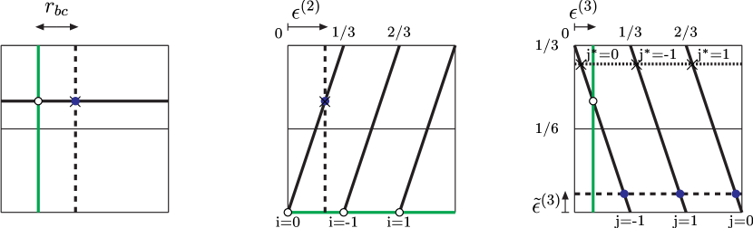
Figure 12: Brane configuration in the model discussed in the text. The leptonic sector is not represented while the baryonic, left, right and orientifold image of the right are respectively the dark solid, faint solid, dashed and dotted. The intersections corresponding to the quark doublets ($i=-1,0,1$), up type singlets ($j=-1,0,1$) and down type singlets ($j^{\ast}=-1,0,1$) are denoted by an empty circle, full circle and a cross, respectively. All distance parameters are measured in units of $2\pi R$ with $R$ the corresponding radius (except $\tilde{\epsilon}^{(3)}$ which is measured in units of $6\pi R$).

The open string light spectrum in these models consists of the following fields:

• $(p+1)$-dimensional gauge bosons (for the case of a stack of $N$ D$p$-branes) corresponding in general to the group $\mathrm{U}(N)\sim\mathrm{SU}(N)\times\mathrm{U}(1)$ live in the world volume of the corresponding branes. In our particular configuration, we have seven-dimensional gauge bosons corresponding to the gauge group $\mathrm{SU}(3)\times\mathrm{SU}(2)\times\mathrm{U}(1)_{a}\times\mathrm{U}(1)_{c}\times\mathrm{U}(1)_{d}$ (see Table 1) . Of the several abelian groups, every anomalous linear combination receives a mass through the Green-Schwartz mechanism, whereas anomaly-free combinations can remain massless or not, depending on the particular brane configuration. This is indeed a salient feature of this class of models that allow non-anomalous gauge bosons to couple to the RR two-form fields acquiring a mass of the order of the string scale in this form [28]. The phenomenology of these extra massive $\mathrm{U}(1)^{\prime}$s has been studied in [37] finding a bound on the string scale $M_{s}\gtrsim 1$ TeV. Interestingly enough, these gauge symmetries remain at the perturbative level as unbroken global symmetries [28]. Quite generally these new global symmetries correspond to baryon, lepton, or Peccei-Quinn like symmetries, preventing proton decay even in low scale models. In our particular example, the anomaly free massless combination corresponding to the hypercharge is

  $$Q_{Y}=\frac{1}{6}Q_{a}-\frac{1}{2}(Q_{c}+Q_{d}).$$

• Four-dimensional chiral massless fermions living on the intersections of two branes and transforming as bi-fundamentals of the corresponding gauge groups. Their number depend on a topological invariant, the intersection number, which in the case of factorizable cycles on a factorizable torus is simply

  $$\mathcal{I}_{ab}=\prod_{I=1}^{3}(n^{I}_{a}m^{I}_{b}-m^{I}_{a}n^{I}_{b}),$$

  with different signs corresponding to different chiralities. The fact that these branes wrap compact dimensions naturally provide intersection numbers greater than one and therefore replication of fermions with the same quantum numbers. It should be mentioned here that in the case of lower-dimensional branes, like D5 or D4-branes, chirality is not automatic and locating the whole configuration at orbifold singularities is required in order to get it [26].

• Four-dimensional scalars, also localized at the intersections, with masses that depend on the particular configurations of the branes. They can be seen as the (generally massive when SUSY is broken by the intersection) superpartners of the fermions at the intersections. In realistic models, scalars with the quantum numbers of the (MS)SM Higgs boson also exist. In the example we are considering the configuration is such that the same supersymmetry is preserved at each of the intersections and massless scalars, superpartners of the corresponding fermions completing the matter spectrum of the MSSM live at the intersections.

The massive spectrum comprises, apart from the winding modes, that correspond to stretched strings that wind around the compact dimensions and have masses $M_{wind}\sim R_{c}/L_{s}^{2}$, where $R_{c}$ is the compactification radius and $L_{s}$ the string scale, KK modes, that are states with non-zero (quantized in units of $1/R_{c}$ due to the periodicity conditions) momentum in the compact dimensions and string excitations not related to the intersections normally present in string models, a set of massive vector-like fermions, the so-called gonions [26], localized near the intersections and with angle-dependent masses. Although a purely effective field theory study shows that relatively light vector-like fermions, especially when they mix with the top quark, are the most likely source of modifications of trilinear couplings [38], the presence of Flavour Changing Neutral Currents (FCNC) in these models overcomes in general any phenomenological relevance of these states.

We have therefore seen that at the level of the light spectrum, models with intersecting branes have a number of nice features, namely four-dimensional chiral fermions, natural family replication and local and global symmetries and matter content of the SM (or simple extensions thereof). As we have seen, the closed string sector, which lives in the full ten-dimensional target space, contains among other fields the graviton. These models thus have a natural hierarchy of dimensionalities, with gravity propagating in ten dimensions, gauge interactions in seven and matter in four. As we sketched in the introduction, this will allow us to reduce the string scale down to observable levels.

In our particular example, as can be seen in Fig. 12, there are no dimensions transverse to all the branes and therefore no transverse volume can be made large enough to account for the large effective four-dimensional Planck mass with a small string scale. The thing that is stopping us are of course the gauge couplings which would receive the same volume suppression seen in Eq. (9) and become extremely small. This problem can be circumvented in several ways, the simplest one is to connect our small torus to a large volume manifold without affecting the brane structure [39], for instance, cutting a hole and sewing and large volume manifold in a region away from the branes . This approach is in spirit quite similar to the bottom-up approach. A second possibility is to consider lower-dimensional branes, for which transverse dimensions to all branes do exist. Realistic examples with D5-branes and a string scale as low as few TeV have been constructed in [40]. (See also [41] for other examples with extra vector-like fermions.) In these models the effective four-dimensional Planck mass reads

$$M_{Pl}=\frac{2}{\lambda_{II}}M_{s}^{4}\sqrt{V_{4}V_{2}},$$ (17)

where $V_{4,2}$ stand for the volume of the four-dimensional manifold where the branes wrap and the volume of the two-dimensional one transverse to all the branes and $\lambda_{II}$ is the string coupling and $M_{s}$ is the string scale. In this situation it is possible to have all scales of order TeV but the transverse dimensions then have to be $\sim$ mm [1].

Gauge couplings can be simply computed from a dimensional reduction of the Yang-Mills theory living on the world-volume of the stack of branes. As expected, it is suppressed by the volume of the compact dimensions of the brane,

$$\frac{1}{g_{a}^{2}}=\frac{M_{s}^{3}}{16\pi^{4}\lambda_{II}}V_{a},$$ (18)

where we have considered the case at hand, i.e. D6-branes wrapping 3-cycles on the compact space and considered the gauge coupling of an $\mathrm{SU}(N_{a})$ group. Reasonable values for the couplings are obtained if the relevant volume for the brane is $V_{a}\sim M_{Pl}^{3}\sim\mathrm{TeV}^{3}$. Contrary to the original expectation, under certain mild assumptions, gauge coupling unification can be obtained [42] (see also [43] for a study of gauge threshold corrections in intersecting brane models).

Models with intersecting branes therefore allow in principle for a very low string scale, $M_{s}\sim 1$ TeV, while keeping the Planck mass (17) and the gauge couplings (18) at the observed values. Notice as well that in the case of non-supersymmetric models, a low string scale is preferred to avoid large corrections to the Higgs vev.

We have not elaborated on the details of the construction and their consistency conditions such as the absence of Ramond-Ramond tadpoles or the presence of unbroken supersymmetries. These conditions greatly restrict the number of possibilities, usually requiring the presence of more complicated spaces by further orbifolding the toroidal structure we have discussed. See for instance [44] for a nice review of this and other related topics.

Among the many phenomenological implications of low scale models, flavour physics is one of the most pressing, so it is to flavour that we now turn. Flavour experiments are typically able to probe mass scales much higher than the energy of current experiments and as we will see shortly this is particularly true in the case of intersecting brane models. The flavour structure of these models is not restricted to Yukawa couplings but flavour violating four-fermion contact interactions are also present at the classical level, giving them a quite unique rich structure. Nonetheless, since both sources of flavour violation are intimately related we shall start with the description of Yukawa couplings.

5.1 Yukawa couplings

The leading contribution to Yukawa couplings between two fermions and a scalar, each living at a different intersection, is due to world-sheet instantons [26]. One can think of this as the classical action for a stretched string leaving an intersection (with one end on each brane) and travelling to the opposite corners of the Yukawa triangle. The action for a string is the worldsheet area, and therefore the amplitude should depend on the area the string sweeps out;

$$Y_{ijk}\sim\mathrm{e}^{-A_{ijk}/\alpha^{\prime}},$$ (19)

where $A_{ijk}$ is the area of the minimal area worldsheet with vertices at the three intersections, bounded by the corresponding branes. (See Fig. 13.)

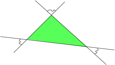
Figure 13: World-sheet instanton contribution to the Yukawa couplings. At each intersection a fermion or a scalar is localized.

A more detailed study of Yukawa couplings, using calibrated geometry [34], and confirmed later by conformal field theory techniques [45], showed that when the compact space is a factorizable torus and the branes wrap factorizable cycles, the relevant area is the sum of the projected areas of the triangle over each sub-torus. The final result, including the quantum part reads

$$Y=\sqrt{2}\lambda_{II}2\pi\sum_{I=1}^{3}\sqrt{\frac{4\pi B(\nu_{I},1-\nu_{I})}{B(\nu_{I},\theta_{I})F(\nu_{I},1-\nu_{I}-\theta_{I})}}\sum_{m}\mathrm{e}^{-\frac{A_{I}(m)}{2\pi\alpha^{\prime}}},$$ (20)

where we have neglected the presence of non-zero $B$ field and Wilson lines and $B$ is the Euler Beta function, $I$ runs over the three tori, $\nu_{I}$ and $\theta_{I}$ are the angles at the fermionic intersections, $m$ runs over all possible triangles connecting the three vertices on each of the three tori (there is an infinite number of them due to the toroidal periodicity) and $A_{I}(m)$ is the projected area of the $m-$th triangle on the $I-$th torus.

This exponential dependence has been claimed as a nice feature of these models since it is expected to naturally give a hierarchical pattern of fermion masses. As we shall see, in practice this does not hold, at least in the simplest models. The reason is that in many cases, the dynamics of left-handed and right-handed fermions turns out to occur in different tori and the property that only the projected triangles are relevant translates into a factorization of the Yukawa couplings. An example is the very model we have been discussing in this section and displayed in detail in Fig. 12. Left-handed quarks live at different points only in the second torus while they live at the same unique intersection in the third one. The opposite happens for right-handed quarks. This results in the following factorizable form of the Yukawa couplings

$$Y^{u}_{ij}=a_{i}b^{u}_{j},\quad Y^{d}_{ij}=a_{i}b^{d}_{j},$$ (21)

where we have only explicitly written the classical part, including this time the presence of non-zero $B-$field and Wilson lines. The coefficients are

$$a_{i} \equiv \vartheta\left[\begin{array}[]{c}\frac{i}{3}+\epsilon^{(2)}\\ \theta^{(2)}\end{array}\right]\Big{(}\frac{3J^{(2)}}{\alpha^{\prime}}\Big{)},$$ (24)

$$b^{u}_{j} \equiv \vartheta\left[\begin{array}[]{c}\frac{j}{3}+\epsilon^{(3)}+\tilde{\epsilon}^{(3)}\\ \theta^{(3)}+\tilde{\theta}^{(3)}\end{array}\right]\Big{(}\frac{3J^{(3)}}{\alpha^{\prime}}\Big{)},$$ (27)

$$b^{d}_{j} \equiv \vartheta\left[\begin{array}[]{c}\frac{j^{\ast}}{3}+\epsilon^{(3)}-\tilde{\epsilon}^{(3)}\\ \theta^{(3)}-\tilde{\theta}^{(3)}\end{array}\right]\Big{(}\frac{3J^{(3)}}{\alpha^{\prime}}\Big{)},$$ (30)

where $i,j,j^{\ast}=-1,0,1$, $J^{(k)}$ denotes the complex Kähler structure of the $k-$th torus, $\theta^{(2)},\theta^{(3)},\tilde{\theta}^{(3)}$ parameterize the Wilson lines and $\vartheta$ is the complex theta function with characteristics, defined as

$$\vartheta\left[\begin{array}[]{c}\delta\\ \phi\end{array}\right](\kappa)=\sum_{l\epsilon Z}\exp[\pi\mathrm{i}(\delta+l)^{2}\kappa+2\pi\mathrm{i}(\delta+l)\phi].$$ (31)

This factorizable form of the Yukawa couplings, Eq. (21), is too simple to lead to a realistic fermion spectrum. It is a rank one matrix with one massive and two massless eigenvalues. There are of course different ways out of this, either by using a more complicated (non-factorizable) compact manifold or by looking for configurations of branes in which the left and right dynamics occur at the same torus. An example of the latter has been provided recently in [36], where a three Higgs model with democratic rather than hierarchical Yukawas is studied. There is however another feature of these very simple models that makes the naive assertion above invalid when quantum corrections are taken into account. This new feature is the presence of FCNCs that propagate through quantum loops to the otherwise trivial structure of Yukawa couplings, providing them with enough complexity to give rise to a realistic set of fermion masses and mixing angles .

5.2 Flavour Changing Neutral Currents

We have emphasized in this review that, after the 2nd string revolution, string theory greatly influenced (and in turn received some degree of inspiration from) field theory investigations, particularly in the area of models with extra dimensions. We shall see a salient example of the complementarity between string and field theory in extra dimensions in this section. Models with intersecting D-branes are a stringy realization of the brane world idea, in which four-dimensional fermions live in the boundaries of extra dimensions where gauge bosons are allowed to propagate, these latter dimensions being a further restriction to a submanifold of the full space-time where gravity lives [1, 47]. One well known property of brane worlds in which the different fermions live in separate points of the extra dimensions, the split fermion scenario [48], is the appearance of FCNCs that tightly constraint the compactification scale $M_{C}\gtrsim 10^{2-3}$ TeV in the case of flat extra dimensions [49] . (See also [51] for a model with light vector-like fermions, relevant for phenomenology despite this very large compactification scale.) The origin of these FCNC can be simply traced to the fact that Kaluza-Klein modes of the multi-dimensional gauge bosons, having a non-trivial profile in the extra dimensions, couple in a different way to the fermions localized at the different positions. Family non-universal gauge bosons then induce FCNC in the fermion mass eigenstate basis [52]. Gauge boson KK generated FCNC are therefore expected from a purely field theory viewpoint in models with intersecting D-branes. A string calculation of the tree level four-fermion amplitude, which can be performed [45] using an extension of the conformal field theory techniques developed for the heterotic orbifolds [53], indeed reproduces the field theory expectation. In addition, though, it reveals a new purely stringy source of flavour violation in these models mediated by string instantons [35]. These are simply worldsheets that directly connect four fermions of different generations living at different intersections in the same way that the Yukawas connected the higgs to two fermions. Again the suppression goes roughly as the area, so that one would expect the FCNC effect from this source to increase as the compactification length and hence worldsheet area decrease.

The KK mediated flavour violating four fermion interactions are of the form,

$$O_{LL}^{(\vec{n})}=\frac{(c_{LL}^{(\vec{n})})_{abcd}}{M_{n}^{2}}(\bar{\psi}_{aL}\gamma^{\mu}\psi_{bL})(\bar{\psi}_{cL}\gamma^{\mu}\psi_{dL}),$$ (32)

with the following dependence of the coefficient

$$(c_{LL}^{(\vec{n})})_{abcd}\sim\delta^{-M_{\vec{n}}^{2}/M_{s}^{2}}\sum_{ij}(U^{\dagger}_{L})_{ai}(U_{L})_{ib}(U^{\dagger}_{L})_{cj}(U_{L})_{jd}\cos\Big{[}\vec{M}_{\vec{n}}\cdot(\vec{y}^{L}_{i}-\vec{y}^{L}_{j})\Big{]}.$$ (33)

$U_{L}$ are the corresponding unitary matrices rotating current eigenstates into mass eigenstates and $\delta$ is an order one (but always larger) number that depends on the specific brane configurations and represents the string smoothing of the KK contribution at high energies which is generally divergent in the field theory calculation of the same effect. (Essentially, the string smoothing arises because the branes have a finite width of order the string length, and are therefore unable to excite modes of a shorter wavelength than this.) We have only written the Left-Left contribution, the case of Right-Right and Left-Right contributions is a straight-forward generalization of that one. Note that in order to have FCNC it is essential that current and mass eigenstates are not aligned (so that the rotation matrices are non-trivial) and the different generations are localized at separate points of the extra dimension ($y_{i}-y_{j}\neq 0$). The exponential smoothing provided by the string dynamics, which is crucial in the case of more than one extra dimensions where the sums over KK modes typically diverge, has to be introduced by hand in a field-theory approach. This is another example of the complementarity between string and field theory. String theory automatically cuts-off the contribution of KK modes heavier than the string scale. Therefore the larger the ratio $R_{c}/L_{s}$, the bigger the number of KK modes that contribute and the larger the effect is.

On the other hand, string instanton FCNCs depend very much on the chiralities of the external fermions (through the difference in the number of independent angles). Four-fermion interactions with all fermions of the same chirality (either all LH or all RH) correspond to a parallelogram with only one independent angle. Given the factorization property of the model we are discussing, the only non-vanishing world-sheet area occurs in one torus and the result is of the form

$$O_{LL}^{str}=\frac{(c_{LL}^{(\vec{n})})_{abcd}}{M_{s}^{2}}(\bar{\psi}_{aL}\gamma^{\mu}\psi_{bL})(\bar{\psi}_{cL}\gamma^{\mu}\psi_{dL}),$$ (34)

with the following dependence of the coefficient

$$(c_{LL}^{str})_{abcd}\sim\mathrm{e}^{-\frac{A}{2\pi L_{s}^{2}}}\sum_{i}(U^{\dagger}_{L})_{ai}(U_{L})_{(i+1)b}(U^{\dagger}_{L})_{c(i+1)}(U_{L})_{(i+2)d},$$ (35)

where $A$ is the area of the corresponding parallelogram (which is $\sim(4\pi^{2}R_{c}^{2})/3$) and $L_{s}=1/M_{s}$ is the string scale. Already in this chirality preserving interaction we observe several differences with respect to the field theory case. The first one is that there are FCNC even in the case of Yukawa couplings aligned with gauge couplings (i.e. $U=1$). Secondly, the exponential dependence on the ratio of string and compactification scales is opposite to that coming from the KK modes, the larger the ratio $R_{c}/L_{S}$, (i.e. the larger the area in string units) the stronger the suppression. Notice however that it is still necessary to have different generations living at separate points in order to have FCNC. The opposite dependence of the KK and string instanton contributions on the ratio of compactification and string scales allows us to put a lower bound on the string scale, independently of this ratio. An estimation of this bound [35], using the KK contribution to $|\epsilon_{K}|$ and the string instanton contribution to $\tau\to ee\mu$ and relatively small mixing angles, leads to the bound $M_{s}\gtrsim 100$ TeV as shown in Fig. 14.

Figure 14: Bound on the string scale as a function of the ratio $L_{c}/L_{s}$ from the KK contribution to $|\epsilon_{K}|$ and the string instanton contribution to $\tau\to ee\mu$. A global bound $M_{s}\gtrsim 100$ TeV is found.

The chirality changing four-fermion interactions, connecting two left-handed and two right-handed fermions, is a bit more involved but far more interesting. We will give the final expressions here and outline the reasons for the new features without entering into the intricacies of the calculation. The main new feature is the absence of L-R factorization in the amplitude (except in some limiting cases). The reason is that now in general there are non-zero contributions in more than one 2-torus and the classical action is no longer the sum of the areas of each of the quadrangles (incidentally, this does not happen for the Yukawa couplings because in the three-point amplitude we can fix all three vertices using $SL(2,R)$ invariance whereas in the four-point one we have to integrate over the position of the fourth vertex, see [54].) As we shall see soon, this introduces enough flavour violation to generate, through loop corrections, a semi-realistic pattern of fermion masses and mixing angles.

Another nice feature with possible important phenomenological implications is related to Higgs-mediated like processes. Let us consider the situation displayed in Fig. 15. The Higgs mediated process can be obtained as the field theory limit of a string propagating from the vertices 2 and 3 down to the Higgs vertex and then back to the vertices 1 and 4. This contribution goes, in the $t$ channel, like

$$\frac{\mathrm{e}^{-A_{23H}/2\pi L_{s}^{2}}\mathrm{e}^{-A_{14H}/2\pi L_{s}^{2}}}{t-M_{H}^{2}}\sim\frac{Y_{23}Y_{14}}{t-M_{H}^{2}},$$ (36)

where $M_{H}$ is the Higgs mass. On the other hand there is another, purely stringy contribution (not expected on field theory grounds) that can be very much enhanced for a low string scale and corresponds to a string sweeping out the area of the quadrangle between the four vertices 1,2,3,4 without going through the Higgs vertex (shaded area in the Figure). In this case if all the flavour dynamics happens on a single torus the amplitude goes as

$$\frac{\mathrm{e}^{-A_{1234}/2\pi L_{s}^{2}}}{M_{s}^{2}}\sim\frac{Y_{23}/Y_{14}}{M_{s}^{2}}.$$ (37)

If the flavour dynamics happens in more than one torus the detailed result depends on the particular configuration due to the non-factorization property of this four point amplitude alluded to above, but is roughly the same. A more detailed study is necessary before making any statement about the phenomenological implications of this property but it seems that a general feature of models with intersecting branes is the presence of Higgs-like processes enhanced (as opposite to the usual expected suppression) by light Yukawas.

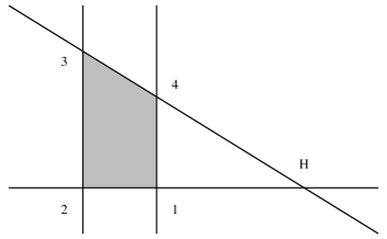
Figure 15: Higgs vs string instanton mediation of the process $(\bar{q}_{aL}q_{bR})(\bar{q}_{cR}q_{dL})$

Let us now concentrate on the relevant amplitude for the generation of fermion masses and mixing angles. In particular we will consider the quark sector and are interested on the $(\bar{q}_{aL}q_{bR})(\bar{q}_{cR}q_{dL})$ amplitude. The full expressions are intricate and do not admit a simple analytical form. In order to give some feeling of what happens we will consider a simplified case in which the relevant angles are the same on each sub-torus. In this case the classical action turns out to be [45]

$$S_{cl}=\frac{1}{4\pi\alpha^{\prime}}\frac{\sin\pi\vartheta_{2}\sin\pi\vartheta_{3}}{\sin(\pi\vartheta_{2}+\pi\vartheta_{3})}\sqrt{\sum_{m}(v_{23}^{m}-v_{14}^{m})^{2}\sum_{n}(v_{23}^{n}-v_{14}^{n})^{2}},$$ (38)

where $\theta_{2,3}$ are the (independent) angles at the corresponding intersections and $v_{23}$, $v_{14}$ are the distances between the relevant intersections. From this expression it is clear that only in the trivial case (when $a=d$ or $b=c$) or in the degenerate case (when distances in all sub-tori are equal) the amplitude $\sim\exp(-S_{cl})$ factorizes.

We have discussed the different tree-level contributions to the flavour structure of models with intersecting branes. Let us consider now how this highly non-trivial structure of flavour violation propagates, through quantum corrections to the otherwise trivial (at tree level) Yukawa couplings.

5.3 Yukawa couplings at one loop

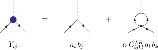
Figure 16: One loop threshold correction to Yukawa couplings. The black dot represents the insertion of a flavour violating four-fermion contact interaction.

Let us recapitulate the main features of the model we are considering. Tree level Yukawa couplings factorize in left and right parts, leading to a rank one matrix of the form

$$Y^{u}_{ij}=a_{i}b^{u}_{j},\quad Y^{d}_{ij}=a_{i}b^{d}_{j}.$$ (39)

On the other hand, four-fermion contact interactions violate flavour at tree level. In particular there is a chirality changing contribution that does not factorize except at particularly symmetric points. One then expects that this non-trivial flavour structure propagates at the quantum level to the Yukawa couplings as sketched in Fig. 16. The expected one loop value or the Yukawa couplings is

$$Y_{ij}\sim a_{i}b_{j}+\alpha C^{LR}_{ijkl}a_{l}b_{k}+\ldots$$ (40)

where we have loosely denoted by $\alpha$ the loop suppression and $C^{LR}_{ijkl}\sim\exp(-S_{cl})$ with the classical action similar to the one in Eq. (38).

Note that there is another one loop contribution to the Yukawa couplings mediated by KK gauge bosons that we are neglecting for simplicity . This and other, higher loop, corrections would be necessary in the case that the LR string contribution factorized, the Yukawa coupling would be in this case still a rank two matrix and therefore those corrections would be essential to give masses to the first generation. In general this contribution does not factorize though and we can generate the full fermionic spectrum with just this leading effect. In order to get approximate analytical expressions we will assume that there is a small deviation on $C^{LR}$ from factorization,

$$C^{LR}_{ijkl}a_{l}b_{k}=c_{i}d_{j}+\epsilon\tilde{C}^{LR}_{ij},$$ (41)

where $\tilde{C}^{LR}$ is a general matrix and $\epsilon$ is a small parameter. The full Yukawa matrix can then be written, at one loop order, as

$$Y^{u,d}_{ij}=a_{i}b^{u,d}_{j}+\alpha c_{i}d^{u,d}_{j}+\alpha\epsilon\tilde{C}^{u,dLR}_{ij}.$$ (42)

This matrix can be perturbatively diagonalized by the following unitary matrices,

$$L^{u,d}=L_{0}\begin{pmatrix}1-\Big{(}\frac{\mu_{12}^{u,d}}{\mu_{1}^{u,d}}\Big{)}^{2}\epsilon^{2}&\frac{\mu_{12}^{u,d}}{\mu_{1}^{u,d}}\epsilon&\alpha\epsilon\frac{\mu^{u,d}_{13}}{|a||b^{u,d}|}\\ -\frac{\mu_{12}^{u,d}}{\mu_{1}^{u,d}}\epsilon&1-\Big{(}\frac{\mu_{12}^{u,d}}{\mu_{1}^{u,d}}\Big{)}^{2}\epsilon^{2}&\alpha\frac{\mu^{u,d}_{2}}{|a||b^{u,d}|}\\ \alpha\epsilon\frac{\mu^{u,d}_{12}\mu^{u,d}_{2}/\mu^{u,d}_{1}-\mu^{u,d}_{13}}{|a||b^{u,d}|}&-\alpha\frac{\mu^{u,d}_{2}}{|a||b^{u,d}|}&1\end{pmatrix},$$ (43)

and a similar rotation for the right handed fields. The order one rotation reads

$$L_{0}=\Big{(}\frac{\vec{a}\wedge\vec{c}}{|\vec{a}\wedge\vec{c}|},\frac{(\vec{a}\cdot\vec{c})\vec{a}-a^{2}\vec{c}}{|(\vec{a}\cdot\vec{c})\vec{a}-a^{2}\vec{c}|},\frac{\vec{a}}{|a|}\Big{)},$$ (44)

and the resulting mass eigenstates are, to leading order,

$$M^{u,d}=\frac{v^{u,d}}{\sqrt{2}}\begin{pmatrix}\alpha\epsilon\mu^{u,d}_{11}&&\\ &\alpha\mu^{u,d}_{1}&\\ &&|a||b^{u,d}|\end{pmatrix},$$ (45)

where we have included the vev of the up or down Higgs, related by $\tan\beta$. Finally, the $(12),(13)$ and $(23)$ entries of the CKM miximg matrix, $V^{CKM}=L^{u\,\dagger}L^{d}$, are

$$V^{CKM}_{12}= \epsilon\Big{[}\frac{\mu^{d}_{12}}{\mu^{d}_{1}}-\frac{\mu^{u}_{12}}{\mu^{u}_{1}}\Big{]},$$

$$V^{CKM}_{13}= \alpha\epsilon\frac{1}{|a|}\Big{[}\frac{\mu^{u}_{12}\mu^{u}_{2}/\mu^{u}_{1}-\mu^{u}_{13}}{|b^{u}|}-\frac{\mu^{u}_{12}\mu^{d}_{2}/\mu^{u}_{1}-\mu^{d}_{13}}{|b^{d}|}\Big{]}$$

$$V^{CKM}_{23}= \alpha\frac{1}{|a|}\Big{[}\frac{\mu^{d}_{2}}{|b^{d}|}-\frac{\mu^{u}_{2}}{|b^{u}|}\Big{]}.$$

The different coefficients in the previous equations are

$$\mu_{1}^{u,d}=\frac{|\vec{a}\wedge\vec{c}||\vec{b}^{u,d}\wedge\vec{d}^{u,d}|}{|\vec{a}||\vec{b}^{u,d}|},\quad\mu_{2}^{u,d}=-\frac{|\vec{a}\wedge\vec{c}|(\vec{b}^{u,d}\cdot\vec{d}^{u,d})}{|\vec{a}||\vec{b}^{u,d}|},$$ (46)

and

$$\mu^{u,d}_{ij}=(L_{0}^{\dagger}\tilde{C}^{LR}R_{0})_{ij},$$ (47)

all expected to be order one. The hierarchical pattern of quark masses and mixing angles found in nature [55]

$$m_{u}\sim 3\times 10^{-3}\mbox{ GeV},\quad m_{c}\sim 1.2\mbox{ Gev},\quad m_{t}\sim 174\mbox{ GeV},$$

$$m_{d}\sim 7\times 10^{-3}\mbox{ GeV},\quad m_{s}\sim 0.12\mbox{ Gev},\quad m_{b}\sim 4.2\mbox{ GeV},$$ (48)

$$V_{12}\sim 0.22,\quad V_{13}\sim 0.0035,\quad V_{23}\sim 0.04,$$

can be explained by a hierarchy in the expansion coefficients, $\alpha$ and $\epsilon$. In fact reasonable values for all experimental data in Eq. (48), up to order one coefficients, can be obtained using,

$$\alpha\sim 10^{-2},\quad\epsilon\sim 0.1,$$ (49)

but for the up quark for which some amount of cancelation seems necessary.

5.4 Experimental bounds on the string scale

Once we have developed a semi-realistic theory of flavour in a concrete model with intersecting branes we can estimate the contribution to flavour violating processes (such as rare decays, meson oscillations, etc.) and extract from them stringent experimental bounds on the string scale for these models. Although a definite pattern for the fermion spectrum along the lines outline above has not yet been fully developed, estimates using the one and two loops KK contribution to the Yukawa couplings [56], leads to the bounds on the string scale shown in Table 2.

Quark sector		Semileptonic Observables
Observable	$M_{s}\gtrsim$ (TeV)	Observable	$M_{s}\gtrsim$ (TeV)
$\Delta m_{K}$	4000	$\mu-e$ conversion	2700
$\Delta m_{B_{d}}$	1300	$K\to\mu\mu$	80
$\Delta m_{B_{s}}$	500	$K\to\pi\mu\mu$	200
$\Delta m_{D}$	2000	Supernovi	10
$|\epsilon_{K}|$	$10^{4}$
Hg EDM	10

Table 2: Bounds on the string scale from different observables in the quark (left) and leptonic (right) sectors. The observables in the upper part are CP preserving while the ones in the lower part of the table are CP violating.

In this table CP conserving quark observables are considered in the upper left side. In the lower left side, we include quark CP violating observables whereas the right side is devoted to semileptonic observables. The bounds should be taken with caution. First, a fully realistic example of fermion masses and mixing angles generation along the lines above has not been produced yet and the detailed value of the FCNC present in the model depends as we saw on the rotation matrices and therefore on the Yukawa couplings . Second, in the estimates of Ref. [56], only the quark sector was considered, and CP violation was neglected. This means that the very stringent bounds should be taken as estimates of the order of magnitude of the result in a more realistic calculation, and are more precise in the CP conserving quark sector than in the rest. Nevertheless it is clear that the bounds are so constraining that it does not seem feasible to have models of intersecting branes with a very low string scale. Equivalently we can say that flavour observables are probing string scales of the order of $M_{s}\gtrsim 10^{3-4}$ TeV.

These bounds have been obtained for a very particular intersecting brane model. The presence of FCNC is however quite general in these models (unless we require all three families to live at the same intersection in which case we loose some of the nice features of these models such as family replication of generations or hierarchical Yukawa couplings) and although model dependent, it is natural to expect a bound on the string scale of the same order of magnitude for a wide variety of models with branes intersecting at non-trivial angles, because of the different origin and moduli dependence of the various sources of flavour violation together with the fact that flavour-violating observables are so restricted experimentally. Therefore we seem to be forced back to high string scales solely on experimental grounds. A great deal of effort has been dedicated to the study of realistic supersymmetric models (in order to protect the hierarchy of scales) with a high string scale, of the order of the Planck or GUT scales [23, 31] and it seems likely that it is to these that we must now turn.

6 Conclusions

In this paper we have described in some detail the way in which string theory has been able to accommodate the most esoteric of theoretical ideas, that of large extra dimensions or low fundamental scales. Here the approach we have taken is to show how string theory has developed alongside the more generic ideas to do with extra dimensions that have been proposed in a purely field theoretic set-up. Beginning with the Horava-Witten set-up which incorporated a fundamental scale of $\sim 10^{16}$ GeV, the construction of models involving D-branes has allowed set-ups first with an intermediate fundamental scale of $\sim 10^{11}$ GeV and later with fundamental scales of $\sim 1$ TeV. The latter realized in string theory the ideas put forward in ref. [1] for solving the hierarchy problem. The large Planck scale was in this scenario put down to the large volume of some compactified space rather than any fundamental hierarchies of scale. The question of fine-tuning could then be shifted onto the various moduli fields that describe how large the compact space is, where (it is hoped) one might be able to exercise more control.

There are a number of aspects that we have touched on and that we would like to reemphasize here. The most important we feel is the fact that the stringy constructions have had to conform to the strictures imposed upon them by the various dualities inherent in string theory. This makes them far more constrained than might have been expected and certainly more constrained than the field theory equivalents. For example we have shown how flavour changing (FCNC) experiments in fact rule out the low scale string models and actually probe models with string scales all the way up to $10^{7}$ GeV. In a sense this makes the string approach more honest. In a field theoretic set-up it often seems to be possible to avoid experimental bounds by retiring to some corner of parameter space. In string theory such corners tend not to exist. A good example of this is the FCNC effect of Kaluza-Klein modes that were considered. In field theory one can reduce the size of the relevant dimensions to make the modes heavy and turn this source of FCNC off. In string theory however this merely introduces compensating FCNCs due to string instanton effects.

One further aspect we touched upon in the context of the intermediate models, is that stringy set-ups may introduce a reasonable explanation for some parameters that are apparently fine-tuned (i.e. unnatural in the sense of t’Hooft). The particular example we chose was the phenomenon of Kinetic-Mixing leading to just the right mediation of D-term supersymmetry breaking. Although this is encouraging, we think that one has to be rather careful in the interpretation; there is no such thing as a free lunch. What really happened in this case is that the fine-tuning of the Kinetic-Mixing was tied to the volume suppression of the gravitational interactions. In the end the number of fine-tunings is reduced but one is still left with the problem of fine-tuning the large volume. This aspect of large extra-dimensions and low fundamental scales has to wait until a better understanding of the behaviour of moduli fields and in particular supersymmetry breaking.

References

- [1] N. Arkani-Hamed, S. Dimopoulos and G. R. Dvali, Phys. Lett. B 429 (1998) 263 [arXiv:hep-ph/9803315]; I. Antoniadis, N. Arkani-Hamed, S. Dimopoulos and G. R. Dvali, Phys. Lett. B 436 (1998) 257 [arXiv:hep-ph/9804398]; N. Arkani-Hamed, S. Dimopoulos and G. R. Dvali, Phys. Rev. D 59 (1999) 086004 [arXiv:hep-ph/9807344].
- [2] P. Horava and E. Witten, Nucl. Phys. B460 (1996) 506; Nucl. Phys. B475 (1996) 94.
- [3] J. Polchinski, arXiv:hep-th/9611050; C.V.Johnson, D-branes, CUP (2003)
- [4] E. G. Gimon and J. Polchinski, Phys. Rev. D 54 (1996) 1667 [arXiv:hep-th/9601038].
- [5] G. Aldazabal, L. E. Ibanez, F. Quevedo and A. M. Uranga, JHEP 0008, 002 (2000) [arXiv:hep-th/0005067].
- [6] K. Benakli, Phys. Rev. D 60, 104002 (1999) [arXiv:hep-ph/9809582]; C. P. Burgess, L. E. Ibanez and F. Quevedo, Phys. Lett. B 447, 257 (1999) [arXiv:hep-ph/9810535].
- [7] W. Fischler and L. Susskind, Phys. Lett. B 171, 383 (1986); Phys. Lett. B 173, 262 (1986)
- [8] S.A.Abel, B.C.Allanach, F.Quevedo, L.Ibanez, M.Klein, JHEP 0012:026,2000
- [9] B.Holdom, Phys.Lett.B166:196,1986
- [10] S. Davidson, S. Hannestad and G. Raffelt, JHEP 0005, 003 (2000) [arXiv:hep-ph/0001179]; S. Davidson and M. E. Peskin, Phys. Rev. D 49, 2114 (1994) [arXiv:hep-ph/9310288].
- [11] S. A. Abel and B. W. Schofield, Nucl. Phys. B 685 (2004) 150 [arXiv:hep-th/0311051].
- [12] K. R. Dienes, C. F. Kolda and J. March-Russell, Nucl. Phys. B 492 (1997) 104 [arXiv:hep-ph/9610479].
- [13] L. E. Ibanez, C. Munoz and S. Rigolin, Nucl. Phys. B 553 (1999) 43 [arXiv:hep-ph/9812397].
- [14] B.C.Allanach, C.G. Lester, M.A.Parker, B.R. Webber, JHEP 0009:004,2000; D.Bailin, G.V.Kraniotis, A. Love, Phys.Lett.B491:161-171,2000
- [15] E. Gabrielli, S. Khalil, C. Munoz, E. Torrente-Lujan, Phys.Rev.D63:025008,2001; A. Bottino, F. Donato, N. Fornengo, S. Scopel, Phys.Rev.D63:125003,2001; D.G. Cerdeno, E. Gabrielli, S. Khalil, C. Munoz, E. Torrente-Lujan, Nucl.Phys.B603:231-258,2001; S. Khalil, C. Munoz, E. Torrente-Lujan, New J.Phys.4:27,2002
- [16] D.G.Cerdeno, E.Gabrielli, S.Khalil, C.Munoz, E.Torrente-Lujan, Phys.Rev.D64:093012,2001; S.Baek, P. Ko, H.S. Lee, Phys.Rev.D65:035004,2002; S.Baek, P.Ko, W.Y. Song, JHEP 0303:054,2003
- [17] J-M.Frere, D.R.T.Jones and S.Raby, Nucl.Phys.B222 (1983)11; M.Claudson, L.Hall and I.Hinchcliffe, Nucl.Phys.B228 (1983)501; H-P.Nilles, M.Srednicki and D.Wyler, Phys.Lett.B120 (1983)346; J-P.Derendinger and C.A.Savoy, Nucl.Phys.B237 (1984) 307.
- [18] Alejandro Ibarra, JHEP 0201:003,2002
- [19] S. A. Abel and B. C. Allanach, JHEP 0007 (2000) 037 [arXiv:hep-ph/9909448].
- [20] G.L. Kane, J. Lykken, B.D. Nelson, L-T Wang, Phys.Lett.B551:146-160,2003
- [21] M. Berkooz, M. R. Douglas and R. G. Leigh, Nucl. Phys. B 480 (1996) 265 [arXiv:hep-th/9606139].
- [22] C. Bachas, arXiv:hep-th/9503030.
- [23] M. Cvetic, G. Shiu and A. M. Uranga, Phys. Rev. Lett. 87, 201801 (2001) [arXiv:hep-th/0107143]; M. Cvetic, G. Shiu and A. M. Uranga, Nucl. Phys. B 615, 3 (2001) [arXiv:hep-th/0107166]; M. Cvetic, G. Shiu and A. M. Uranga, arXiv:hep-th/0111179; D. Cremades, L. E. Ibanez and F. Marchesano, JHEP 0207, 009 (2002) [arXiv:hep-th/0201205]; M. Cvetic, P. Langacker and G. Shiu, Phys. Rev. D 66, 066004 (2002) [arXiv:hep-ph/0205252]; R. Blumenhagen, L. Gorlich and T. Ott, JHEP 0301 (2003) 021 [arXiv:hep-th/0211059]; M. Cvetic, I. Papadimitriou and G. Shiu, arXiv:hep-th/0212177; G. Honecker, Nucl. Phys. B 666, 175 (2003) [arXiv:hep-th/0303015]; M. Cvetic and I. Papadimitriou, Phys. Rev. D 67, 126006 (2003) [arXiv:hep-th/0303197]; M. Cvetic, P. Langacker and J. Wang, Phys. Rev. D 68, 046002 (2003) [arXiv:hep-th/0303208]; K. Behrndt and M. Cvetic, arXiv:hep-th/0308045; C. Kokorelis, arXiv:hep-th/0309070.
- [24] R. Blumenhagen, L. Goerlich, B. Kors and D. Lust, JHEP 0010 (2000) 006 [arXiv:hep-th/0007024].
- [25] S. Forste, G. Honecker and R. Schreyer, JHEP 0106, 004 (2001) [arXiv:hep-th/0105208].
- [26] G. Aldazabal, S. Franco, L. E. Ibanez, R. Rabadan and A. M. Uranga, J. Math. Phys. 42 (2001) 3103 [arXiv:hep-th/0011073]; G. Aldazabal, S. Franco, L. E. Ibanez, R. Rabadan and A. M. Uranga, JHEP 0102 (2001) 047 [arXiv:hep-ph/0011132].
- [27] R. Blumenhagen, L. Gorlich, B. Kors and D. Lust, Nucl. Phys. B 582 (2000) 44 [arXiv:hep-th/0003024]; S. Forste, G. Honecker and R. Schreyer, Nucl. Phys. B 593 (2001) 127 [arXiv:hep-th/0008250].
- [28] L. E. Ibanez, F. Marchesano and R. Rabadan, JHEP 0111 (2001) 002 [arXiv:hep-th/0105155].
- [29] R. Rabadan, Nucl. Phys. B 620 (2002) 152 [arXiv:hep-th/0107036]; R. Blumenhagen, B. Kors, D. Lust and T. Ott, Nucl. Phys. B 616 (2001) 3 [arXiv:hep-th/0107138]; G. Honecker, JHEP 0201, 025 (2002) [arXiv:hep-th/0201037]; R. Blumenhagen, D. Lust and T. R. Taylor, Nucl. Phys. B 663 (2003) 319 [arXiv:hep-th/0303016].
- [30] D. Cremades, L. E. Ibanez and F. Marchesano, JHEP 0207, 022 (2002) [arXiv:hep-th/0203160].
- [31] C. Kokorelis, JHEP 0208 (2002) 018 [arXiv:hep-th/0203187]; JHEP 0209 (2002) 029 [arXiv:hep-th/0205147]; JHEP 0208 (2002) 036 [arXiv:hep-th/0206108]; arXiv:hep-th/0207234; JHEP 0211 (2002) 027 [arXiv:hep-th/0209202]; arXiv:hep-th/0210200; arXiv:hep-th/0212281; M. Axenides, E. Floratos and C. Kokorelis, arXiv:hep-th/0307255;
- [32] J. R. Ellis, P. Kanti and D. V. Nanopoulos, Nucl. Phys. B 647 (2002) 235 [arXiv:hep-th/0206087].
- [33] J. Garcia-Bellido, R. Rabadan and F. Zamora, JHEP 0201 (2002) 036 [arXiv:hep-th/0112147]; R. Blumenhagen, B. Kors, D. Lust and T. Ott, Nucl. Phys. B 641 (2002) 235 [arXiv:hep-th/0202124]; M. Gomez-Reino and I. Zavala, JHEP 0209 (2002) 020 [arXiv:hep-th/0207278].
- [34] D. Cremades, L. E. Ibanez and F. Marchesano, JHEP 0307 (2003) 038 [arXiv:hep-th/0302105].
- [35] S. A. Abel, M. Masip and J. Santiago, JHEP 0304 (2003) 057 [arXiv:hep-ph/0303087].
- [36] N. Chamoun, S. Khalil and E. Lashin, arXiv:hep-ph/0309169.
- [37] D. M. Ghilencea, L. E. Ibanez, N. Irges and F. Quevedo, JHEP 0208 (2002) 016 [arXiv:hep-ph/0205083]; D. M. Ghilencea, Nucl. Phys. B 648 (2003) 215 [arXiv:hep-ph/0208205].
- [38] F. del Aguila, M. Perez-Victoria and J. Santiago, Phys. Lett. B 492 (2000) 98 [arXiv:hep-ph/0007160]; F. del Aguila, M. Perez-Victoria and J. Santiago, JHEP 0009 (2000) 011 [arXiv:hep-ph/0007316].
- [39] R. Blumenhagen, V. Braun, B. Kors and D. Lust, JHEP 0207 (2002) 026 [arXiv:hep-th/0206038]; A. M. Uranga, JHEP 0212 (2002) 058 [arXiv:hep-th/0208014].
- [40] D. Cremades, L. E. Ibanez and F. Marchesano, Nucl. Phys. B 643 (2002) 93 [arXiv:hep-th/0205074].
- [41] D. Bailin, G. V. Kraniotis and A. Love, Phys. Lett. B 530 (2002) 202 [arXiv:hep-th/0108131]; D. Bailin, G. V. Kraniotis and A. Love, Phys. Lett. B 547 (2002) 43 [arXiv:hep-th/0208103]; D. Bailin, G. V. Kraniotis and A. Love, Phys. Lett. B 553 (2003) 79 [arXiv:hep-th/0210219]. D. Bailin, G. V. Kraniotis and A. Love, JHEP 0302 (2003) 052 [arXiv:hep-th/0212112].
- [42] R. Blumenhagen, D. Lust and S. Stieberger, JHEP 0307 (2003) 036 [arXiv:hep-th/0305146].
- [43] D. Lust and S. Stieberger, arXiv:hep-th/0302221.
- [44] A. M. Uranga, Class. Quant. Grav. 20, S373 (2003) [arXiv:hep-th/0301032].
- [45] M. Cvetic and I. Papadimitriou, Phys. Rev. D 68 (2003) 046001 [arXiv:hep-th/0303083]; S. A. Abel and A. W. Owen, Nucl. Phys. B 663 (2003) 197 [arXiv:hep-th/0303124]; and to appear
- [46] S. A. Abel, O. Lebedev and J. Santiago, arXiv:hep-ph/0312157.
- [47] V. A. Rubakov and M. E. Shaposhnikov, Phys. Lett. B 125 (1983) 136; I. Antoniadis, Phys. Lett. B 246 (1990) 377; I. Antoniadis and K. Benakli, Phys. Lett. B 326 (1994) 69 [arXiv:hep-th/9310151]; A. Pomarol and M. Quiros, Phys. Lett. B 438 (1998) 255 [arXiv:hep-ph/9806263].
- [48] N. Arkani-Hamed and M. Schmaltz, Phys. Rev. D 61 (2000) 033005 [arXiv:hep-ph/9903417].
- [49] A. Delgado, A. Pomarol and M. Quiros, JHEP 0001 (2000) 030 [arXiv:hep-ph/9911252]; C. D. Carone, Phys. Rev. D 61 (2000) 015008 [arXiv:hep-ph/9907362].
- [50] S. J. Huber, Nucl. Phys. B 666 (2003) 269 [arXiv:hep-ph/0303183].
- [51] F. Del Aguila and J. Santiago, JHEP 0203 (2002) 010 [arXiv:hep-ph/0111047].
- [52] P. Langacker and M. Plumacher, Phys. Rev. D 62 (2000) 013006 [arXiv:hep-ph/0001204].
- [53] L. J. Dixon, D. Friedan, E. J. Martinec and S. H. Shenker, Nucl. Phys. B 282 (1987) 13; S. Hamidi and C. Vafa, Nucl. Phys. B 279 (1987) 465.
- [54] A. Owen, talk at String Phenomenology 2003.
- [55] K. Hagiwara et al. (Particle Data Group), Phys. Rev. D66, 010001 (2002)
- [56] J. Santiago, talk at String Phenomenology 2003.