Thermal pion masses in the second phase: $|\mu_{I}|>m_{\pi}$

Abstract

Density and thermal corrections to the mass of the pions are studied in the framework of the $SU(2)$ low energy effective chiral lagrangian, in terms of the isospin chemical potential $\mu_{\mbox{\tiny$I$}}$. We concentrate the discussion in the region where the isospin chemical potential (absolute value) becomes bigger than the pion mass at zero temperature and density, i.e. in the phase where the condensed $\pi^{-}$ phase appears (for negative chemical potential). We are able to calculate the thermal and density evolution of masses in the limits where $|\mu_{I}|\gg m$ and where $|\mu_{I}|\ \gtrsim m$. We also identified the phase transition curve.

In this paper we continue with the discussion of the thermal and density pion properties that we started in Loewe:2002tw ; Loewe:2003dq now in the so called second phase where the absolute value of the isospin chemical potential becomes bigger than the tree-level pion mass at zero temperature and density. In the first phase, unless we go to the chiral limit, the Isospin symmetry $SU(2)$ is broken due to mass effects. This effect, as soon as we take $|\mu_{I}|>m_{\pi}$ becomes extremely important since one of the charged pions condense. Here we will use the following definition of the isospin chemical potential $\mu_{\mbox{\tiny$I$}}\equiv\mu_{u}-\mu_{d}$, being $\mu_{u,d}$ the chemical potential corresponding to the baryon number of the up and down quarks. In the case of pions, the isospin chemical potential will correspond essentially to the difference between the number of positive and negative charged pions.

We recall that pion masses at finite temperature $m_{\pi}(T)$ have been studied in a variety of frameworks, such as thermal QCD-Sum Rules Dominguez:1996kf , Chiral Perturbation Theory ($\chi$PT) (low temperature expansion) Gasser:1986vb , the Linear Sigma Model Larsen:1985ei ; Contreras:1989gi , the Mean Field Approximation Barducci:1991rh , the Virial Expansion Schenk:1991xe , etc. In fact, the pion propagation at finite temperature has been calculated at two loops in the frame of $\chi$PT Schenk:1993ru ; Toublan:1997rr . In our article, we follow the way of introducing chemical potentials in $\chi$PT that was presented for the first time in Kogut:1999iv ; Kogut:2000ek . Even though, these articles deal with QCD with two colors rather than QCD with three colors, it is clear that both problems are intimately related.

The introduction of in-medium processes via isospin chemical potential has been studied at zero temperature Son:2000xc ; Son:2000by ; Kogut:2001id in both phases ($|\mu_{\mbox{\tiny$I$}}|\lessgtr m_{\pi}$) at tree level. In medium properties at finite density have been discussed for a variety of phenomena, as for example, the chiral condensates Peng:2003jh ; Peng:2003nq , the anomalous decays of pions and etas As the density increases both, the quark condensates and the decay rates diminish.

Interesting results concerning the structure of the QCD phase diagram, including temperature effects have been achieved for the case when we have simultaneously various baryon chemical potential and isospin chemical potential simultaneously. Two completely different approaches have confirmed a qualitative change in the phase diagram as soon as the isospin chemical potential starts to grow Toublan:2003tt ; Barducci:2003un . These problems concerning the structure of the phase transition diagram, have been also handle in the frame of two color QCD in four dimensions Splittorff:2002xn as well as in three dimensions Dunne:2003ji . The problem with baryonic chemical potential has been considered in the frame of $\chi$PT Alvarez-Estrada:1995mh , and also using the finite pion number chemical potential Ayala:2002qy .

Different properties of QCD (or QCD-inspired models) under these kind of circumstances have also been analyzed in the lattice approach. For QCD with three and two colors, an extensive work has been carried out Kogut:2001if ; Kogut:2002tm ; Kogut:2002zg ; Kogut:2002cm ; Kogut:2003ju , in connection with the behavior of different order parameters in several phase transitions in the $\mu/T$ plane, as for example, the transition to a diquark phase, the chiral condensate, etc.

A common feature of all approaches in the second phase is the fact that the physical pion states do not correspond anymore to the usual pion charged states. In fact as we will see, the $\pi_{\mbox{\tiny$\pm$}}$ states will mix in a non trivial way. The result of this mixture produces an extremely cumbersome propagator, a matrix $2\times 2$, so we need to define some criteria how to handle this propagator, according to the value of the chemical potential, for computing radiative corrections.

This paper is organized as follows: First we briefly present the chiral lagrangian we will use, specifying the lagrangians of second and fourth order, in the momentum expansion. Then we present our criteria to expand the mass corrections in a Taylor series, in two different limits: a) when the chemical potential is a little bit bigger than the the pion mass and b) in the region where the chemical potential is much bigger than the pion mass. In both limits we will work at the lowest order in our expansion. This will allow us to make a selection of the vertices that will appear in the different diagrams. We have to note, however, that our procedure is only valid for values of the chemical potential up to the mass of the $\eta$ meson. Beyond this point an $SU(3)$ chiral lagrangian is needed. After the selection of relevant vertices, we compute the thermal mass corrections from the propagators at the one loop level. We employ the usual momentum or energy expansion of the propagators around the tree level mass. This will allow us to comment on the phase transition due to the pion condensation and compare with similar results from other authors, Splittorff:2002xn . Finally we present our conclusions.

I The chiral lagrangian

The procedure we will follow is basically the same of Loewe:2002tw ; Loewe:2003dq . The only modification will be the inclusion of non trivial vacuum expectation values for the pion fields. Nevertheless, this is not just a little detail since the discussion becomes much more technically involved and subtle.

In the low-energy description where only pion degrees of freedom are relevant, the most general chiral invariant lagrangian at the second order, ${\cal O}(p^{2})$, according to an expansion in powers of the external momentum is given by

$${\cal L}_{2}=\frac{f^{2}}{4}Tr\left[(D_{\mu}U)^{\dagger}D^{\mu}U+2BM(U^{\dagger}+U)\right]$$ (1)

with

$$D_{\mu}U = \partial_{\mu}U-i\mu_{\mbox{\tiny$I$}}u_{\mu}[\textstyle{\frac{1}{2}}\tau_{3},U]$$

$$U = \bar{U}^{\frac{1}{2}}(e^{i\pi^{a}\tau^{a}/f})\bar{U}^{\frac{1}{2}},$$ (2)

where $\bar{U}$ is the vacuum expectation value of the field $U$. $M=diag(m_{u},m_{d})$ is the quark mass matrix and $B$ in the previous equation is an arbitrary constant which will be fixed when the mass is identified setting $(m_{u}+m_{d})B=m^{2}$, where $m$ denotes the bare (tree-level) pion mass. We will use $m_{\pi}$ to denote the pion masses after renormalization.

The most general ${\cal O}(p^{4})$ chiral lagrangian has the form

$${\cal L}_{4} = \textstyle{\frac{1}{4}}l_{1}\left(Tr\left[(D_{\mu}U)^{\dagger}D^{\mu}U\right]\right)^{2}$$ (3)

$$+\textstyle{\frac{1}{4}}l_{2}Tr\left[(D_{\mu}U)^{\dagger}D_{\nu}U\right]Tr\left[(D^{\mu}U)^{\dagger}D^{\nu}U\right]$$

$$+\textstyle{\frac{1}{4}}(l_{3}+l_{4})B^{2}\left(Tr\left[M(U^{\dagger}+U)\right]\right)^{2}$$

$$+\textstyle{\frac{1}{4}}l_{4}BTr\left[(D_{\mu}U)^{\dagger}D^{\mu}U\right]Tr\left[M(U^{\dagger}+U)\right]$$

$$-\textstyle{\frac{1}{4}}l_{7}B^{2}\left(Tr\left[M(U^{\dagger}-U)\right]\right)^{2}$$

$$+\mbox{constants}.$$

We have used the constants $l_{i}$ introduced by Gasser and Leutwyler, Gasser:1983yg for an $SU(2)$ Lagrangian. They have to be determined experimentally and are also tabulated in several articles and books. This Lagrangian includes the chemical potentials in the covariant derivatives and in the expectation value of the $\bar{U}$ matrix. The constants $l_{i}$ include divergent corrections which allow to cancel the divergences from loops corrections

$$l_{i}(\Lambda)=\frac{\gamma_{i}}{32\pi^{2}}\left[\bar{l}_{i}-\lambda+\ln\left(\frac{m^{2}}{\Lambda^{2}}\right)\right]$$ (4)

with the $\overline{ms}$ pole

$$\lambda=\frac{2}{4-d}+\ln 4\pi+\Gamma^{\prime}(1)+1.$$ (5)

For $|\mu_{\mbox{\tiny$I$}}|>m$ there is a symmetry breaking. The vacuum expectation value that minimizes the potential, calculated in , is

$$\bar{U} = \textstyle{\frac{m^{2}}{\mu_{\mbox{\tiny$I$}}^{2}}}+i[\tau_{1}\cos\phi+\tau_{2}\sin\phi]\sqrt{1-\textstyle{\frac{m^{4}}{\mu_{\mbox{\tiny$I$}}^{4}}}}$$ (6)

$$\equiv c+i\tilde{\tau}_{1}s,$$

where $c\equiv\frac{m^{2}}{\mu_{\mbox{\tiny$I$}}^{2}}$, $s\equiv\sqrt{1-\textstyle{\frac{m^{4}}{\mu_{\mbox{\tiny$I$}}^{4}}}}$. From now, we will refer with a tilde to any vector rotated in a $\phi$ angle

$$\tilde{v}_{1} = v_{1}\cos\phi+v_{2}\sin\phi$$

$$\tilde{v}_{2} = -v_{1}\sin\phi+v_{2}\cos\phi.$$ (7)

The expanded Lagrangian, keeping all the details, is given by

$${\cal L}_{2,2} = \textstyle{\frac{1}{2}}(\partial\bm{\pi})^{2}-\textstyle{\frac{1}{2}}\mu_{\mbox{\tiny$I$}}^{2}(s^{2}\tilde{\pi}_{{\mbox{\tiny$1$}}}^{2}+\pi_{{\mbox{\tiny$3$}}}^{2})-|\mu_{\mbox{\tiny$I$}}|c(\tilde{\pi}_{{\mbox{\tiny$1$}}}\partial_{{\mbox{\tiny$0$}}}\tilde{\pi}_{{\mbox{\tiny$2$}}}-\tilde{\pi}_{{\mbox{\tiny$2$}}}\partial_{{\mbox{\tiny$0$}}}\tilde{\pi}_{{\mbox{\tiny$1$}}})$$

$${\cal L}_{2,3} = \frac{1}{f}|\mu_{\mbox{\tiny$I$}}|s\big{[}(\tilde{\pi}_{{\mbox{\tiny$1$}}}^{2}+\pi_{{\mbox{\tiny$3$}}}^{2})\partial_{{\mbox{\tiny$0$}}}\tilde{\pi}_{{\mbox{\tiny$2$}}}-\textstyle{\frac{1}{2}}|\mu_{\mbox{\tiny$I$}}|c\tilde{\pi}_{{\mbox{\tiny$1$}}}\bm{\pi}^{2}\big{]}$$

$${\cal L}_{2,4} = \frac{1}{f^{2}}\frac{1}{6}\Big{\{}\big{[}-(\partial\bm{\pi})^{2}+\mu_{\mbox{\tiny$I$}}^{2}(s^{2}\tilde{\pi}_{{\mbox{\tiny$1$}}}^{2}+\pi_{{\mbox{\tiny$3$}}}^{2}-\textstyle{\frac{3}{4}}c^{2}\bm{\pi}^{2})+2|\mu_{\mbox{\tiny$I$}}|c(\tilde{\pi}_{{\mbox{\tiny$1$}}}\partial_{{\mbox{\tiny$0$}}}\tilde{\pi}_{{\mbox{\tiny$2$}}}-\tilde{\pi}_{{\mbox{\tiny$2$}}}\partial_{{\mbox{\tiny$0$}}}\tilde{\pi}_{{\mbox{\tiny$1$}}})\big{]}\bm{\pi}^{2}+(\bm{\pi}\cdot\partial\bm{\pi})^{2}\Big{\}}$$

$${\cal L}_{4,1} = \frac{1}{f}\mu_{\mbox{\tiny$I$}}^{4}cs[4s^{2}(l_{1}+l_{2})-2c^{2}l_{3}-s^{2}l_{4}]\tilde{\pi}_{{\mbox{\tiny$1$}}}$$

$${\cal L}_{4,2} = \frac{1}{f^{2}}\mu_{\mbox{\tiny$I$}}^{2}\Big{\{}2s^{2}\big{[}(\partial\bm{\pi})^{2}+2(\partial_{{\mbox{\tiny$0$}}}\tilde{\pi}_{{\mbox{\tiny$2$}}})^{2}\big{]}l_{1}+2s^{2}\big{[}(\partial_{{\mbox{\tiny$0$}}}\bm{\pi})^{2}+(\partial\tilde{\pi}_{{\mbox{\tiny$2$}}})^{2}+(\partial_{{\mbox{\tiny$0$}}}\tilde{\pi}_{{\mbox{\tiny$2$}}})^{2}\big{]}l_{2}+\mu_{\mbox{\tiny$I$}}^{2}c^{2}\epsilon_{{\mbox{\tiny$ud$}}}^{2}\pi_{3}^{2}l_{7}$$ (8)

$$\quad-2s^{2}\big{[}8|\mu_{\mbox{\tiny$I$}}|c\tilde{\pi}_{{\mbox{\tiny$1$}}}\partial_{0}\tilde{\pi}_{{\mbox{\tiny$2$}}}+\mu_{\mbox{\tiny$I$}}^{2}(s^{2}\bm{\pi}^{2}-3c^{2}\tilde{\pi}_{{\mbox{\tiny$1$}}}^{2}-\tilde{\pi}_{{\mbox{\tiny$2$}}}^{2})\big{]}(l_{1}+l_{2})+\mu_{\mbox{\tiny$I$}}^{2}c^{2}\big{[}s^{2}\tilde{\pi}_{{\mbox{\tiny$1$}}}^{2}-c^{2}\bm{\pi}^{2}\big{]}l_{3}$$

$$\quad+\big{[}c^{2}(\partial\bm{\pi})^{2}+2|\mu_{\mbox{\tiny$I$}}|c(1-3c^{2})\tilde{\pi}_{{\mbox{\tiny$1$}}}\partial_{{\mbox{\tiny$0$}}}\tilde{\pi}_{{\mbox{\tiny$2$}}}-\mu_{\mbox{\tiny$I$}}^{2}c^{2}\{(s^{2}+1)\bm{\pi}^{2}-(c^{2}-s^{2})\tilde{\pi}_{{\mbox{\tiny$1$}}}^{2}-\tilde{\pi}_{{\mbox{\tiny$2$}}}^{2}\}\big{]}l_{4}\Big{\}},$$

where the index $n,m$ refers to ${\cal O}(p^{n}),{\cal O}(\pi^{n})$ and $\epsilon_{{\mbox{\tiny$ud$}}}^{2}=(m_{u}-m_{d})^{2}/(m_{u}+m_{d})^{2}$. Note that we use a negative chemical potential ($\mu_{\mbox{\tiny$I$}}=-|\mu_{\mbox{\tiny$I$}}|$) as it is the case in neutron stars where there exist a condensate of $\pi_{-}$ cuasiparticles. The same happens for the $\pi_{+}$ changing the sign of $\mu_{\mbox{\tiny$I$}}$.

From this lagrangian we are able to extract the different vertices that will participate in the diagrams responsible for mass renormalization. Note that in the second phase, there will appear vertices with three legs from (${\cal L}_{2,3}$) and one leg from (${\cal L}_{4,1}$). The last one is responsible for the counterterms of the tadpoles, but in the approximation we will use, these will not be considered, since tadpoles, being of higher orders in the expansion parameter, will be absent as we will see.

II Self-energy in two different limits: $|\mu_{\mbox{\tiny$I$}}|\gtrsim m$, and $|\mu_{\mbox{\tiny$I$}}|\gg m$

In $\chi$PT the natural scale parameter is $\Lambda_{\chi}=4\pi f$, where $f$ is a parameter which at tree level coincides with the pion decay constant. Usually $\Lambda_{\chi}$ is compared with the tree level pion mass defining in this way the smallness parameter for perturbative expansions ($\alpha=(\frac{m}{4\pi f})^{2}$). Now, since $|\mu_{\mbox{\tiny$I$}}|>m$ in the second phase, we will re-define the smallness parameter as

$$\nu=\left(\frac{\mu_{\mbox{\tiny$I$}}}{4\pi f}\right)^{2}$$ (9)

This is possible for values of the chemical potential less than $m_{\eta}$. For higher values in energy parameters we need to consider the $SU(3)$ case.

The inverse of the free propagator for pions in momentum space, i.e. the equations of motion extracted from ${\cal L}_{2,2}$ is given by the matrix

$$i\bm{D}^{-1}=\left(\begin{array}[]{ccc}p^{2}-\mu_{\mbox{\tiny$I$}}^{2}s^{2}&2i|\mu_{\mbox{\tiny$I$}}|cp_{0}&0\\ -2i|\mu_{\mbox{\tiny$I$}}|cp_{0}&p^{2}&0\\ 0&0&p^{2}-\mu_{\mbox{\tiny$I$}}^{2}\end{array}\right),$$ (10)

where

$$\bm{D}_{ij}^{-1}=i\int d^{4}xe^{ipx}\frac{\delta^{2}S[\pi]}{\delta\pi_{{\mbox{\tiny$i$}}}\delta\pi_{{\mbox{\tiny$j$}}}}(x).$$ (11)

The masses are defined as the poles of the determinant of the propagator matrix at zero 3-momentum, i.e. the solution of

$$\left|\bm{D^{-1}}(p)\right|_{\vec{p}=0}=0$$ (12)

We can identify the $\pi_{3}=\pi_{0}$ field, as it is indicated in Kogut:2001id , through its mass at $|\mu_{\mbox{\tiny$I$}}|=m$ and because it is diagonal in the propagator matrix. Therefore, there will be no difficulties to handle this propagator. This is not the case for the charged pions which are mixed in a non trivial way.

The free propagator for the charged pions in momentum space is

$$\tilde{\bm{D}}=\frac{i}{[p^{4}-p^{2}\mu_{\mbox{\tiny$I$}}^{2}s^{2}-4\mu_{\mbox{\tiny$I$}}^{2}c^{2}p_{0}^{2}]}\left(\begin{array}[]{cc}p^{2}&-2i|\mu_{\mbox{\tiny$I$}}|cp_{0}\\ 2i|\mu_{\mbox{\tiny$I$}}|cp_{0}&p^{2}-\mu_{\mbox{\tiny$I$}}^{2}s^{2}\\ \end{array}\right)$$ (13)

with $\tilde{\bm{D}}_{ij}\equiv\bm{D}_{ij\neq 3}$. The Dolan-Jackiw propagators can be constructed with the general formula

$$\bm{D}(p;T) = \int\frac{dk_{0}}{2\pi i}\lim_{\eta\to 0}\frac{\big{[}\bm{D}(k_{0}+i\eta,\bm{p})-\bm{D}(k_{0}-i\eta,\bm{p})\big{]}}{k_{0}-p_{0}-i\epsilon}$$

$$\quad+n_{B}(p_{0})\big{[}\bm{D}(p_{0}+i\epsilon,\bm{p})-\bm{D}(p_{0}-i\epsilon,\bm{p})\big{]}.$$

The main difficulty with this matrix propagator is that it is very cumbersome to integrate the different loop corrections. This fact motivated us to proceed in a systematic way, through an expansion in a new appropriate smallness parameter, namely $s$ when $|\mu_{\mbox{\tiny$I$}}|\gtrsim m$ and $c$ when $|\mu_{\mbox{\tiny$I$}}|\gg m$. We realized that a similar expansion was proposed earlier by Splittorff, Toublan and Verbaarschot Splittorff:2001fy ; Splittorff:2002xn .

It is not difficult to realize that the different vertices which appear in our lagrangian will correspond to different powers of $c$ or $s$ depending on the case. Although it could appear as a trivial correction, we will keep only the zero order in our calculations. As we will see, this procedure is not trivial at all and provides us with interesting information about the behavior of the pion masses as function of temperature and isospin chemical potential.

If we scale all the parameters with $|\mu_{\mbox{\tiny$I$}}|$ in all structures, we have that:

Propagators

$$D(p;T,\mu_{\mbox{\tiny$I$}};m)=\frac{1}{\mu_{\mbox{\tiny$I$}}^{2}}\bar{\bm{D}}(\bar{p};\bar{T},c)$$ (15)

${\cal L}_{4}$ constants

$$l_{i}(\Lambda)=\frac{\gamma_{i}}{32\pi^{2}}\left[\bar{l}_{i}-\lambda-\ln(c\bar{\Lambda}^{2})\right]$$ (16)

Vertices

$$V_{n,m}(p;\mu_{\mbox{\tiny$I$}};f,m,\Lambda)=\frac{|\mu_{\mbox{\tiny$I$}}|^{n}}{f^{m+n-4}}v_{n,m}(\bar{p};\bar{\Lambda},c)$$ (17)

Integrals

$$\int\frac{d^{d}k}{(2\pi)^{d}}\Lambda^{4-d}=\mu_{\mbox{\tiny$I$}}^{4}\int\frac{d^{d}\bar{k}}{(2\pi)^{d}}\bar{\Lambda}^{4-d}$$ (18)

Self-energy

$$\Sigma(p_{0};T,\mu_{\mbox{\tiny$I$}};f,m,\Lambda)=\mu_{\mbox{\tiny$I$}}^{2}\nu\sigma(\bar{p}_{0};\bar{T},c;\bar{\Lambda})$$ (19)

where from now on the bar on a parameter means that it is scaled with $|\mu_{\mbox{\tiny$I$}}|$. It is possible then to expand the propagator in powers of $s^{n}$ for$|\mu_{\mbox{\tiny$I$}}|\gtrsim m$ and $c^{n}$ when $|\mu_{\mbox{\tiny$I$}}|\gg m$.

After the renormalization procedure, the divergent terms and the scale factor $\lambda+\ln\bar{\Lambda}$ that will appear in the loops calculation due to dimentional regularization and the ${\cal L}_{4}$ terms will cancel. Finally the renormalized self-energy will get the form

$$\begin{split}\Sigma_{R}\big{|}_{|\mu_{\mbox{\tiny$I$}}|\gtrsim m}=&\quad\mu_{\mbox{\tiny$I$}}^{2}\nu\sum_{n=0}\sigma_{n}^{(s)}(\bar{p};\bar{T})s^{n}\\ \Sigma_{R}\big{|}_{|\mu_{\mbox{\tiny$I$}}|\gg m}=&\quad\mu_{\mbox{\tiny$I$}}^{2}\nu\sum_{n=0}\big{[}\sigma_{n}^{(c)}(\bar{p};\bar{T})+\sigma^{\mbox{\tiny log}}_{n}(\bar{p})\ln c\big{]}c^{n}.\end{split}$$ (20)

As we said before we will keep only the $n=0$ terms in the previous expansions. This approximation is certainly non trivial since it allows us to explore the behavior of the renormalized masses precisely in the vicinity of the transition point and also in the region of the high chemical potential values. Further corrections could also be calculated, taking into account higher order vertices and propagators. We will consider these in a further discussion.

Obviously, $c$ and $s$ must be smaller than the intersection point $\frac{1}{\sqrt{2}}$. The idea is to find a region around the intersection point that can be excluded safely from both expansions. This excluded area becomes smaller when $n$ (the order of the expansion) starts to grow. By demanding that $c^{n+1},s^{n+1}\lesssim\frac{1}{2}(\frac{1}{\sqrt{2}})^{n+1}$, we achieve this condition. Note that if $n=0$, we would exclude the region of the chemical potential where $\sqrt{\frac{8}{7}}m^{2}\lesssim\mu_{\mbox{\tiny I}}^{2}\lesssim\sqrt{8}m^{2}$. We remark again that by going to higher orders in our expansion, the excluded region becomes smaller, so this is the best bound.

Note that bare masses (tree level masses) in this phase are functions of the chemical potential as was discussed in Kogut:2001id

$$m_{0} = |\mu_{\mbox{\tiny$I$}}|$$

$$m_{+} = |\mu_{\mbox{\tiny$I$}}|\sqrt{1+3c^{2}}$$

$$m_{-} = 0.$$ (21)

As the neutral pion propagator is diagonal with respect to the charged ones, it’s propagator will be the same in both limits at any order:

$$D_{{\mbox{\tiny$00$}}}(p;T)=\frac{i}{p^{2}-\mu_{\mbox{\tiny$I$}}^{2}+i\epsilon}+2\pi n_{B}(|p_{0}|)\delta(p^{2}-\mu_{\mbox{\tiny$I$}}^{2}).$$ (22)

III Renormalization and masses

The corrected propagator is

$$\bm{D}_{c} = \bm{D}-i\bm{D}\bm{\Sigma}\bm{D}+\cdots$$

$$= \bm{D}(1+i\bm{\Sigma}\bm{D})^{-1}$$

$$\bm{D}_{c}^{-1} = \bm{D}^{-1}+i\bm{\Sigma}.$$ (23)

Following the usual renormalization procedure, i.e. re-scaling the fields $\pi_{i}=\sqrt{Z_{i}}\pi_{i}^{r}$ with $Z_{i}=1+{\cal O}(\nu)$ we have that

$$iD_{R}^{-1}(p)_{\mbox{\tiny$ij$}} = Z_{ij}iD^{-1}(p)_{\mbox{\tiny$ij$}}-\Sigma(p)_{\mbox{\tiny$ij$}}+{\cal O}(\nu^{2})$$ (24)

$$= iD^{-1}(p)_{\mbox{\tiny$ij$}}-\Sigma_{R}(p)_{\mbox{\tiny$ij$}}$$

with $Z_{ij}\equiv\sqrt{Z_{i}Z_{j}}$. The value of $Z$ is chosen in such a way that the corrected propagator does not have corrections proportional to $p^{2}$.

As an example, let consider a free propagator and the self energy correction of the form

$$iD^{-1}(p) = p^{2}-2bp_{0}-a^{2}$$

$$\Sigma(p) = \Sigma^{\mbox{\tiny$0$}}+\Sigma^{\mbox{\tiny$1$}}p_{0}+\Sigma^{\mbox{\tiny$2$}}p^{2}.$$ (25)

This expression for $\Sigma$ is valid in the first phase and we will see that it is also valid in the second phase, up to ${\cal O}(s^{0})$.

Choosing $Z=1+\Sigma^{2}$ we have that the renormalized self-energy will be

$$\Sigma_{R}(p) = \big{(}\Sigma^{\mbox{\tiny$0$}}+a^{2}\Sigma^{\mbox{\tiny$2$}}\big{)}+\big{(}\Sigma^{\mbox{\tiny$1$}}+2b\Sigma^{\mbox{\tiny$2$}}\big{)}p_{0}$$ (26)

$$= \Sigma_{R}^{\mbox{\tiny$0$}}+\Sigma_{R}^{\mbox{\tiny$1$}}p_{0}.$$

Unfortunately, in general, the self-energy $\Sigma$ will not have the shape of eq.(25), but it will be a complicated function of the external momenta. As we want to compute mass corrections, it is possible to expand the self energy in terms of these corrections. In the rest frame, where $\bm{p}=0$, the energy will be $p_{0}=m_{R}=m_{t}+\delta m$, where $m_{R}$ is the renormalized mass, $m_{t}$ is the tree level mass and $\delta m$ is the correction due to the self-energy terms. Then

$$\Sigma(m_{R}) = \Sigma(m_{t})+\Sigma^{\prime}(m_{t})\delta m+\textstyle{\frac{1}{2}}\Sigma^{\prime\prime}(m_{t})(\delta m)^{2}+\dots$$

$$= \Sigma^{\mbox{\tiny$0$}}[m_{t}]+\Sigma^{1}[m_{t}]m_{R}+\Sigma^{\mbox{\tiny$2$}}[m_{t}]m_{R}^{2}+{\cal O}(\delta m)^{3}$$

where the mass inside the brackets is the mass around which the self-energy expansion was computed.

As we said in eq.(12), the masses are defined as the poles of the determinant of the corrected propagator matrix at $\bm{p}=0$. In the case of the neutral pion, since it does not mix with the other terms, it is very easy to find the mass correction as the solution of $D_{R}^{-1}(p_{0})_{\mbox{\tiny$00$}}=0$.

As we said before, due to the complicated form of the self-energy, we expand the renormalized mass in the rest frame in powers of the tree-level mass corrections $\delta m$. Since the renormalized massed will be extracted as solutions of

$$\left|\tilde{\bm{D}}^{-1}_{R}(m_{R})\right|\equiv 0,$$ (28)

then we only need to compute the $\delta m$ corrections. This can be done taking an expansion of the determinant up to ${\cal O}(\delta m)^{2}$, which leaves us with a quadratic equation for $\delta m$.

After finding the $\delta m$ corrections, which are of course given in a power series of $\nu$, we can neglect terms of ${\cal O}(\nu^{2})$ in the renormalized mass. Note that for finite tree level masses ($m_{t}\gg\nu|\mu_{\mbox{\tiny I}}|$) it is enough to expand up to ${\cal O}(\delta m)\sim{\cal O}(\nu)$

In the case of the condensed pion, where the tree-level mass vanishes, some care has to be taken because now we do not have a natural dimensionfull quantity to refer to as a scale parameter. Here we will find corrections to the mass, only for finite temperature, in the same way as it occurs for the photon-mass corrections in QED LeBellac:1996 , which in our case will include terms of the form $\sqrt{{\cal O}(\mu_{\mbox{\tiny I}}^{2}\nu)+{\cal O}(\mu_{\mbox{\tiny I}}^{2}\nu^{2})}$.

IV Limit $|\mu_{\mbox{\tiny$I$}}|\gtrsim m$

IV.1 Propagators and vertices ($|\mu_{\mbox{\tiny$I$}}|\gtrsim m$)

Figure 1: Propagators ${\cal O}(s^{0})$

Figure 2: Relevant vertices at ${\cal O}(s^{0})$

The propagator for the charged pions at ${\cal O}(s^{0})$ is given by

$$\tilde{\bm{D}}=\frac{i}{[p^{4}-4\mu_{\mbox{\tiny$I$}}^{2}p_{0}^{2}]}\left(\begin{array}[]{cc}p^{2}&-2i|\mu_{\mbox{\tiny$I$}}|p_{0}\\ 2i|\mu_{\mbox{\tiny$I$}}|p_{0}&p^{2}\\ \end{array}\right)+\frac{1}{\mu_{\mbox{\tiny$I$}}^{2}}{\cal O}(s^{2})$$ (29)

It is more convenient to work with the following combination of fields

$$\tilde{\pi}_{\pm}=\textstyle{\frac{1}{\sqrt{2}}}(\tilde{\pi}_{{\mbox{\tiny$1$}}}\mp i\tilde{\pi}_{{\mbox{\tiny$2$}}}).$$ (30)

We remark that the $\tilde{\pi}_{\pm}$ fields do not correspond to the physical charged pion fields but to a combination of them. This fact is a consequence of the non trivial vacuum structure in this phase. This combination is also not trivial due to derivative terms and the inverse D’alambertian operator. We would like to mention that in the first phase ($\mu_{\mbox{\tiny I}}<m$) the $\pi_{\pm}$ correspond effectively to the charged pions and the propagator becomes anti-diagonal. Then, the equations of motion for charged pions are

$$i\tilde{\bm{D}}^{-1}\!\!\!\! = \!\!\!\!\left(\begin{array}[]{cc}-\textstyle{\frac{1}{2}}\mu_{\mbox{\tiny$I$}}^{2}s^{2}&p^{2}+2|\mu_{\mbox{\tiny$I$}}|cp_{0}-\textstyle{\frac{1}{2}}\mu_{\mbox{\tiny$I$}}^{2}s^{2}\\ &\\ p^{2}-2|\mu_{\mbox{\tiny$I$}}|cp_{0}-\textstyle{\frac{1}{2}}\mu_{\mbox{\tiny$I$}}^{2}s^{2}&-\textstyle{\frac{1}{2}}\mu_{\mbox{\tiny$I$}}^{2}s^{2}\end{array}\right)$$ (34)

$$= i\left(\begin{array}[]{cc}D^{-1}_{\mbox{\tiny$++$}}&D^{-1}_{\mbox{\tiny$+-$}}\\ &\\ D^{-1}_{\mbox{\tiny$-+$}}&D^{-1}_{\mbox{\tiny$--$}}\end{array}\right)$$ (38)

and the free propagator matrix is

$$\tilde{\bm{D}}=i\left(\begin{array}[]{cc}0&\frac{1}{p^{2}-2|\mu_{\mbox{\tiny$I$}}|p_{0}}\\ \frac{1}{p^{2}+2|\mu_{\mbox{\tiny$I$}}|p_{0}}&0\\ \end{array}\right)+\frac{1}{\mu_{\mbox{\tiny$I$}}^{2}}{\cal O}(s).$$ (39)

The Dolan-Jackiw propagators for charged pions, including isospin chemical potential (enough for one loop calculations) are

$$D(p;T)_{{\mbox{\tiny$+-$}}} = \frac{i}{p^{2}-2|\mu_{\mbox{\tiny$I$}}|p_{0}+i\epsilon}$$

$$+2\pi n_{B}(|p_{0}|)\delta(p^{2}-2|\mu_{\mbox{\tiny$I$}}|p_{0})+\frac{1}{\mu_{\mbox{\tiny$I$}}^{2}}{\cal O}(s^{2})$$

$$D(p;T)_{\mbox{\tiny$-+$}} = D(-p;T)_{\mbox{\tiny$+-$}}$$ (40)

and the other propagators, $D_{\mbox{\tiny$++$}}$ and $D_{\mbox{\tiny$--$}}$ are of order $s^{2}$, so we will neglect them. For diagrammatic purposes, the $D_{{\mbox{\tiny$+-$}}}$ propagator will be drawn as an arrow from $+$ to $-$ as appear in FIG. 1.

The relevant vertices at the zero order in this region are shown in FIG. 2, where the corresponding analytical expressions are given by

$$V_{2,4}^{\mbox{\tiny$0000$}} = i\frac{\mu_{\mbox{\tiny I}}^{2}}{f^{2}}\big{[}1+{\cal O}(s^{2})\big{]}$$

$$V_{2,4}^{\mbox{\tiny$00\pm$}} = \frac{i}{3f^{2}}\Big{\{}2p_{{\mbox{\tiny$(0)$}}}q_{{\mbox{\tiny$(0)$}}}+2p_{{\mbox{\tiny$(+)$}}}p_{{\mbox{\tiny$(-)$}}}+|\mu_{\mbox{\tiny I}}|(p_{{\mbox{\tiny$(+)$}}}^{0}-p_{{\mbox{\tiny$(-)$}}}^{0})-\mu_{\mbox{\tiny I}}^{2}-\big{[}p_{{\mbox{\tiny$(0)$}}}+q_{{\mbox{\tiny$(0)$}}}\big{]}\big{[}p_{{\mbox{\tiny$(+)$}}}+p_{{\mbox{\tiny$(-)$}}}\big{]}+\mu_{\mbox{\tiny$I$}}^{2}{\cal O}(s^{2})\Big{\}}$$

$$V_{2,4}^{{\mbox{\tiny$\pm\pm$}}} = \frac{i}{3f^{2}}\Big{\{}\big{[}p_{{\mbox{\tiny$(+)$}}}+q_{{\mbox{\tiny$(+)$}}}\big{]}\big{[}p_{{\mbox{\tiny$(-)$}}}+q_{{\mbox{\tiny$(-)$}}}\big{]}-6\mu_{\mbox{\tiny$I$}}^{2}-4|\mu_{\mbox{\tiny I}}|(p_{{\mbox{\tiny$(+)$}}}^{0}+q_{{\mbox{\tiny$(+)$}}}^{0}-p_{{\mbox{\tiny$(-)$}}}^{0}-q_{{\mbox{\tiny$(-)$}}}^{0})-2p_{{\mbox{\tiny$(+)$}}}q_{{\mbox{\tiny$(+)$}}}-2p_{{\mbox{\tiny$(-)$}}}q_{{\mbox{\tiny$(-)$}}}+\mu_{\mbox{\tiny I}}^{2}{\cal O}(s^{2})\Big{\}}$$

$$V_{4,2}^{{\mbox{\tiny$00$}}} = -i2\frac{\mu_{\mbox{\tiny I}}^{2}}{f^{2}}\big{[}\mu_{\mbox{\tiny I}}^{2}l_{3}+(2pq+\mu_{\mbox{\tiny I}}^{2})l_{4}-\mu_{\mbox{\tiny I}}^{2}\epsilon_{ud}^{2}l_{7}+\mu_{\mbox{\tiny I}}^{2}{\cal O}(s^{2})\big{]}$$

$$V_{4,2}^{{\mbox{\tiny$-+$}}} = -i2\frac{\mu_{\mbox{\tiny I}}^{2}}{f^{2}}\big{[}\mu_{\mbox{\tiny I}}^{2}l_{3}+(p_{{\mbox{\tiny$(+)$}}}p_{{\mbox{\tiny$(-)$}}}+|\mu_{\mbox{\tiny I}}|(p_{{\mbox{\tiny$(+)$}}}^{0}-p_{{\mbox{\tiny$(-)$}}}^{0}))l_{4}+\mu_{\mbox{\tiny$I$}}^{2}{\cal O}(s^{2})\big{]}.$$ (41)

All the momenta emerge from the vertices. In principle, there will appear also other vertices: $v_{2,2}^{{\mbox{\tiny$++$}}}$, $v_{2,2}^{{\mbox{\tiny$--$}}}$, $v_{2,4}^{{\mbox{\tiny$00++$}}}$, $v_{2,4}^{{\mbox{\tiny$00--$}}}$, $v_{2,4}^{{\mbox{\tiny$\pm++$}}}$, $v_{2,4}^{{\mbox{\tiny$\pm--$}}}$ of ${\cal O}(s^{2})$ and $v_{2,3}$, $v_{4,1}$ of ${\cal O}(s)$. As we said, however, since we are working at zero order, this terms will not be considered in our analysis.

IV.2 Self-energy ($|\mu_{\mbox{\tiny$I$}}|\gtrsim m$)

Proceeding with the relevant vertices and propagators the loops corrections to the pion’s propagator matrix are shown in FIG. 3 and FIG. 4

Figure 3: $\Sigma_{{\mbox{\tiny$00$}}}$ at ${\cal O}(s^{0})$

Figure 4: $\Sigma_{{\mbox{\tiny$-+$}}}$ at ${\cal O}(s^{0})$

Defining $\underline{\lambda}=\lambda+\ln\bar{\Lambda}$, the self-energy is

$$\Sigma(p)_{{\mbox{\tiny$00$}}} = \nu\Big{\{}-\mu_{\mbox{\tiny$I$}}^{2}\big{[}\textstyle{\frac{4}{3}}\underline{\lambda}+\textstyle{\frac{1}{2}}\bar{l}_{3}-2\bar{l}_{4}+2I^{\prime}_{0}-\textstyle{\frac{4}{3}}I^{\prime}\big{]}+p^{2}\big{[}\textstyle{\frac{4}{3}}\underline{\lambda}-2\bar{l}_{4}+\textstyle{\frac{8}{3}}I^{\prime}\big{]}+{\cal O}(\mu_{\mbox{\tiny I}}^{2}s^{2})\Big{\}}$$

$$\Sigma(p)_{{\mbox{\tiny$-+$}}} = \nu\Big{\{}-\mu_{\mbox{\tiny$I$}}^{2}\big{[}\textstyle{\frac{1}{2}}\bar{l}_{3}-2I^{\prime}_{0}-8J^{\prime}\big{]}-2p_{0}|\mu_{\mbox{\tiny$I$}}|\big{[}\textstyle{\frac{4}{3}}\underline{\lambda}-2\bar{l}_{4}+\textstyle{\frac{4}{3}}I^{\prime}_{0}+\textstyle{\frac{4}{3}}I^{\prime}+4J^{\prime}\big{]}+p^{2}\big{[}\textstyle{\frac{4}{3}}\underline{\lambda}-2\bar{l}_{4}+\textstyle{\frac{4}{3}}I^{\prime}_{0}+\textstyle{\frac{4}{3}}I^{\prime}\big{]}+{\cal O}(\mu_{\mbox{\tiny I}}^{2}s^{2})\Big{\}}$$

$$\Sigma(p)_{{\mbox{\tiny$+-$}}} = \Sigma(-p)_{{\mbox{\tiny$-+$}}}$$ (42)

with

$$I^{\prime} \equiv \int_{1}^{\infty}dx\sqrt{x^{2}-1}\Big{[}n_{B}\big{(}|\mu_{\mbox{\tiny I}}||x-1|\big{)}+x\rightarrow-x\Big{]}$$

$$J^{\prime} \equiv \int_{1}^{\infty}dx\sqrt{x^{2}-1}\Big{[}xn_{B}\big{(}|\mu_{\mbox{\tiny I}}||x-1|\big{)}+x\rightarrow-x\Big{]}$$

$$I^{\prime}_{n} \equiv \int_{1}^{\infty}dx\sqrt{x^{2}-1}x^{2n}2n_{B}\big{(}|\mu_{\mbox{\tiny$I$}}|x\big{)}.$$ (43)

Note that these definitions are almost the same ones we used in our previous paper Loewe:2002tw ; Loewe:2003dq . Here, however, the term that multiplies $x$ in the argument of the Bose-Einstein distribution is $\mu_{\mbox{\tiny I}}$ instead of $m$. Following the prescription indicated in Section III, that the renormalized self-energy does not depend on $p^{2}$ we have that the renormalization constants are

$$Z_{0} = 1+\nu\big{[}\textstyle{\frac{4}{3}}\underline{\lambda}-2\bar{l}_{4}+\textstyle{\frac{8}{3}}I^{\prime}\big{]}$$

$$Z_{\pm} = 1+\nu\big{[}\textstyle{\frac{4}{3}}\underline{\lambda}-2\bar{l}_{4}+\frac{4}{3}I^{\prime}_{0}+\textstyle{\frac{4}{3}}I^{\prime}\big{]}$$ (44)

and the renormalized self-energy corrections are

$$\Sigma_{R{\mbox{\tiny$00$}}} = \mu_{\mbox{\tiny$I$}}^{2}\nu\big{[}-\textstyle{\frac{1}{2}}\bar{l}_{3}-2I^{\prime}_{0}+4I^{\prime}\big{]}$$

$$\Sigma_{R}(p_{0})_{\mbox{\tiny$-+$}} = \nu\Big{\{}\mu_{\mbox{\tiny$I$}}^{2}\big{[}-\textstyle{\frac{1}{2}}\bar{l}_{3}+2I^{\prime}_{0}+8J^{\prime}\big{]}-8|\mu_{\mbox{\tiny$I$}}|J^{\prime}p_{0}\Big{\}}$$

$$\Sigma_{R}(p_{0})_{\mbox{\tiny$+-$}} = \Sigma_{R}(-p_{0})_{\mbox{\tiny$-+$}}$$ (45)

plus higher corrections of order $\mu_{\mbox{\tiny I}}^{2}\nu s^{2}$. We will use these results to extract the renormalized temperature- and chemical potential-dependent masses.

IV.3 Masses ($|\mu_{\mbox{\tiny$I$}}|\gtrsim m$)

To extract the $m_{\pi^{\mbox{\tiny$0$}}}$ mass, we do not need any further effort since it is already diagonal in the matrix propagator, and it’s renormalized self-energy is constant in the external momenta, i.e., it does not depend on $p_{0}$.

$$m_{\pi^{\mbox{\tiny$0$}}}=|\mu_{\mbox{\tiny I}}|\Big{\{}1+\nu\big{[}-\textstyle{\frac{1}{4}}\bar{l}_{3}-I^{\prime}_{0}+2I^{\prime}\big{]}\Big{\}}.$$ (46)

For the case of $m_{\pi^{\mbox{\tiny$\pm$}}}$, the vanishing determinant of the charged matrix propagator, provides us with a second order equation in powers of $p_{0}^{2}$.

$$p_{0}^{4}-p_{0}^{2}\Big{[}m_{+}^{2}+2\Sigma_{R{\mbox{\tiny$-+$}}}^{\mbox{\tiny$0$}}+4c\Sigma_{R{\mbox{\tiny$-+$}}}^{\mbox{\tiny$1$}}+(\Sigma_{R{\mbox{\tiny$-+$}}}^{\mbox{\tiny$1$}})^{2}\Big{]}$$

$$\qquad+s^{2}\Sigma_{R{\mbox{\tiny$-+$}}}^{\mbox{\tiny$0$}}+(\Sigma_{R{\mbox{\tiny$-+$}}}^{\mbox{\tiny$0$}})^{2}=0.$$ (47)

The solution of this equation gives the $\pi^{\pm}$ masses, recognizing them respectively according to the tree-level case if we set the self-energy corrections to zero. We can write the expression for the masses in a more compact way, by expanding around the $m_{+}$ term that appears in the last equation. Then, the masses are given by

$$m_{\pi^{+}} = m_{+}+\nu|\mu_{\mbox{\tiny I}}|\big{[}-\textstyle{\frac{1}{4}}\bar{l}_{3}+I^{\prime}_{0}-4J^{\prime}+{\cal O}(s^{2})\big{]}$$

$$m_{\pi^{-}} = \textstyle{\frac{1}{2}}|\mu_{\mbox{\tiny I}}|\Big{\{}\big{(}s^{2}+\nu[-\textstyle{\frac{1}{2}}\bar{l}_{3}+2I^{\prime}_{0}+8J^{\prime}]\big{)}$$ (48)

$$\quad\times\nu[-\textstyle{\frac{1}{2}}\bar{l}_{3}+2I^{\prime}_{0}+8J^{\prime}]+{\cal O}(\nu^{2}s^{2})\Big{\}}^{1/2}.$$

As we indicated previously, $m_{\pi^{\mbox{\tiny$-$}}}$ can not be expressed as a sum of some initial mass plus corrections, since it does not have a tree level mass to compare with in the second phase. Thermal radiative corrections, however, will induce a non trivial behavior for the renormalized $m_{\pi^{-}}(T,\mu_{\mbox{\tiny I}})$. It is interesting to remark that $m_{\pi^{\mbox{\tiny$-$}}}$ does not have a finite real solution for $\bar{l}_{3}>4I^{\prime}_{0}+16J^{\prime}$, according to the previous equation. This means that $\pi^{-}$ remains in the condensed state for $T$ less than a certain critical value.

V Limit $|\mu_{I}|\gg m$

V.1 Propagators and vertices ($|\mu_{I}|\gg m$)

Figure 5: Propagators ${\cal O}(c^{0})$

Figure 6: Relevant vertices at ${\cal O}(c^{0})$

Proceeding in the same way as in the $|\mu_{I}|\gtrsim m$ case, the propagator of the charged pions $\tilde{\pi}_{{\mbox{\tiny$1$}}}$ and $\tilde{\pi}_{{\mbox{\tiny$2$}}}$ at zero temperature at ${\cal O}(c^{0})$ is

$$\tilde{\bm{D}}=i\left(\begin{array}[]{cc}\frac{1}{p^{2}-\mu_{I}^{2}}&0\\ 0&\frac{1}{p^{2}}\\ \end{array}\right)+\frac{1}{\mu_{I}^{2}}{\cal O}(c).$$ (49)

The $\pi_{{\mbox{\tiny$0$}}}$ propagator remains the same as the $|\mu_{I}|\gtrsim m$ case in the equation (22). Then, the Dolan-Jackiw propagators for charged pions are

$$\begin{split}D_{{\mbox{\tiny$11$}}}(p;T,|\mu_{\mbox{\tiny I}}|)=&D_{{\mbox{\tiny$00$}}}(p;T,|\mu_{\mbox{\tiny I}}|)+\frac{1}{\mu_{I}^{2}}{\cal O}(c^{2})\\ D_{{\mbox{\tiny$22$}}}(p;T,|\mu_{I}|)=&\frac{i}{p^{2}+i\epsilon}+2\pi n_{B}(|p^{0}|)\delta(p^{2})+\frac{1}{\mu_{I}^{2}}{\cal O}(c^{2})\end{split}$$ (50)

and the propagators $\bar{D}_{{\mbox{\tiny$12$}}}$ and $\bar{D}_{{\mbox{\tiny$21$}}}$ are of order $c$. In the case of a propagator with zero mass, it is necessary to introduce a small fictitious mass as a regulator, i.e. $D_{{\mbox{\tiny$22$}}}^{-1}=\lim_{\eta\to 0}(p^{2}-\eta^{2})$. Note that in the chiral limit ($c=0$) the fields $\pi_{{\mbox{\tiny$1$}}}$ and $\pi_{{\mbox{\tiny$0$}}}$ have the same behavior. The other components of the propagator matrix are of order $c$. Diagrammatically, we will denote the $D_{{\mbox{\tiny$11$}}}$ propagator with a line and $D_{{\mbox{\tiny$22$}}}$ with a dashed line, as we can see in FIG. 5. The $D_{{\mbox{\tiny$00$}}}$ propagator remains the same.

The relevant vertices at ${\cal O}(c^{0})$ are indicated in FIG. 6 with the analytical expressions

$$V_{2,3}^{{\mbox{\tiny$002$}}} = V_{2,3}^{{\mbox{\tiny$112$}}}=\frac{2|\mu_{\mbox{\tiny I}}|}{f}\big{[}p_{\mbox{\tiny$(2)$}}^{0}+{\cal O}(\mu_{\mbox{\tiny I}}c)\big{]}$$

$$V_{2,4}^{{\mbox{\tiny$0000$}}} = i\frac{\mu_{I}^{2}}{f^{2}}[1+{\cal O}(c^{2})]$$

$$V_{2,4}^{{\mbox{\tiny$0011$}}} = \frac{i}{3f^{2}}[2p_{{\mbox{\tiny$(0)$}}}q_{{\mbox{\tiny$(0)$}}}+2p_{{\mbox{\tiny$(1)$}}}q_{{\mbox{\tiny$(1)$}}}+4\mu_{\mbox{\tiny I}}^{2}-(p_{{\mbox{\tiny$(0)$}}}+q_{{\mbox{\tiny$(0)$}}})(p_{{\mbox{\tiny$(1)$}}}+q_{{\mbox{\tiny$(1)$}}})+\mu_{\mbox{\tiny I}}^{2}{\cal O}(c^{2})]$$

$$V_{2,4}^{{\mbox{\tiny$0022$}}} = \frac{i}{3f^{2}}[2p_{{\mbox{\tiny$(0)$}}}q_{{\mbox{\tiny$(0)$}}}+2p_{{\mbox{\tiny$(2)$}}}q_{{\mbox{\tiny$(2)$}}}+2\mu_{\mbox{\tiny I}}^{2}-(p_{{\mbox{\tiny$(0)$}}}+q_{{\mbox{\tiny$(0)$}}})(p_{{\mbox{\tiny$(2)$}}}+q_{{\mbox{\tiny$(2)$}}})+\mu_{\mbox{\tiny I}}^{2}{\cal O}(c^{2})]$$ (51)

$$V_{2,4}^{{\mbox{\tiny$1122$}}} = \frac{i}{3f^{2}}[2p_{{\mbox{\tiny$(1)$}}}q_{{\mbox{\tiny$(1)$}}}+2p_{{\mbox{\tiny$(2)$}}}q_{{\mbox{\tiny$(2)$}}}+2\mu_{\mbox{\tiny I}}^{2}-(p_{{\mbox{\tiny$(1)$}}}+q_{{\mbox{\tiny$(1)$}}})(p_{{\mbox{\tiny$(2)$}}}+q_{{\mbox{\tiny$(2)$}}})+\mu_{\mbox{\tiny I}}^{2}{\cal O}(c^{2})]$$

$$V_{4,2}^{{\mbox{\tiny$00$}}} = i4\frac{\mu_{\mbox{\tiny I}}^{2}}{f^{2}}[(p_{{\mbox{\tiny$(0)$}}}q_{{\mbox{\tiny$(0)$}}}+\mu_{\mbox{\tiny I}}^{2})l_{1}+(p_{{\mbox{\tiny$(0)$}}}^{0}q_{{\mbox{\tiny$(0)$}}}^{0}+\mu_{I}^{2})l_{2}+\mu_{\mbox{\tiny I}}^{2}{\cal O}(c^{2})]$$

$$V_{4,2}^{{\mbox{\tiny$11$}}} = i4\frac{\mu_{\mbox{\tiny I}}^{2}}{f^{2}}[(p_{{\mbox{\tiny$(1)$}}}q_{{\mbox{\tiny$(1)$}}}+\mu_{\mbox{\tiny I}}^{2})l_{1}+(p_{{\mbox{\tiny$(1)$}}}^{0}q_{{\mbox{\tiny$(1)$}}}^{0}+\mu_{\mbox{\tiny I}}^{2})l_{2}+\mu_{\mbox{\tiny I}}^{2}{\cal O}(c^{2})]$$

$$V_{4,2}^{{\mbox{\tiny$22$}}} = i4\frac{\mu_{\mbox{\tiny I}}^{2}}{f^{2}}[(p_{{\mbox{\tiny$(2)$}}}q_{{\mbox{\tiny$(2)$}}}+2p_{{\mbox{\tiny$(2)$}}}^{0}q_{{\mbox{\tiny$(2)$}}}^{0})(l_{1}+l_{2})+\mu_{\mbox{\tiny I}}^{2}{\cal O}(c^{2})].$$

As in the $|\mu_{\mbox{\tiny I}}|\gtrsim m$ case, there will appear also other vertices of higher order in power of $c$: $\bar{V}_{2,2}^{{\mbox{\tiny$$12$$}}}$, $v_{2,3}^{{\mbox{\tiny$$001$$}}}$, $v_{2,3}^{{\mbox{\tiny$$111$$}}}$, $v_{2,3}^{{\mbox{\tiny$$122$$}}}$, $v_{2,4}^{{\mbox{\tiny$$0012$$}}}$, $v_{2,4}^{{\mbox{\tiny$$1112$$}}}$, $v_{2,4}^{{\mbox{\tiny$$1222$$}}}$, $v_{4,2}^{{\mbox{\tiny$$12$$}}}$, of ${\cal O}(c)$.

V.2 Self-Energy ($|\mu_{I}|\gg m$)

Figure 7: $\Sigma_{{\mbox{\tiny$22$}}}$ at ${\cal O}(c^{0})$

Figure 8: $\Sigma_{{\mbox{\tiny$00$}}}$ (or $\Sigma_{{\mbox{\tiny$11$}}}$) at ${\cal O}(c^{0})$

As we did for the $|\mu_{\mbox{\tiny I}}|\gtrsim m$ case, we use the relevant vertices and propagators to compute the self-energy corrections. In our approximation (${\cal O}(c^{0})$), the corrections to the $D_{{\mbox{\tiny$00$}}}$ and $D_{{\mbox{\tiny$11$}}}$ are the same. This happens because their vertices and propagators differ in quantities of order higher than $c$.

The loop corrections are shown in FIG. 8, for $D_{{\mbox{\tiny$11$}}}$ (which are the same as those of $D_{{\mbox{\tiny$00$}}}$ exchanging the single line with the double line), and FIG. 7 for $D_{{\mbox{\tiny$22$}}}$.

Note that in this region tadpole diagrams appear, which are absent in the previous case. However, at the order $c^{0}$, it turns out that these tadpoles vanish, because the vertex is proportional to $p_{0}$, and the tail of the tadpole does not carry momentum. At the order $c$, there will appear non vanishing tadpole diagrams (and also new ${\cal L}_{4}$ corrections). Nevertheless, for high values of the chemical potential, the leading behavior will be given by our approximation.

The self energy corrections are

$$\Sigma(p_{0})_{\mbox{\tiny$00$}} = \nu\mu_{\mbox{\tiny I}}^{2}\Big{\{}(p_{0}^{2}-1)\big{[}\textstyle{\frac{2}{3}}\underline{\lambda}+2\ln c-\textstyle{\frac{2}{3}}\bar{l}_{1}-\textstyle{\frac{4}{3}}\bar{l}_{2}+\textstyle{\frac{4}{3}}+\textstyle{\frac{4}{3}}I^{\prime}_{0}+\textstyle{\frac{4}{9}}\pi^{2}T^{2}\big{]}$$

$$\hskip 28.45274pt+\textstyle{\frac{4}{3}}-4I^{\prime}_{0}+2A_{1}(p_{0})+16B_{0}(p_{0})+16B_{1}(p_{0})-32\pi iC_{1}(p_{0})\Big{\}}$$

$$\Sigma(p_{0})_{\mbox{\tiny$11$}} = \Sigma(p_{0})_{\mbox{\tiny$00$}}$$

$$\Sigma(p_{0})_{\mbox{\tiny$22$}} = 2\nu\mu_{\mbox{\tiny I}}^{2}\Big{\{}p_{0}^{2}\big{[}\textstyle{\frac{2}{3}}\underline{\lambda}-\bar{l}_{1}-2\bar{l}_{2}+3\ln c+2-\textstyle{\frac{4}{3}}I^{\prime}_{0}\big{]}+2A_{2}(p_{0})+16B_{2}(p_{0})-32\pi iC_{2}(p_{0})\Big{\}}$$ (52)

plus corrections of order $\nu\mu_{\mbox{\tiny I}}^{2}c^{2}$. The functions $A_{n}$, $B_{n}$, $C_{n}$ are defined as

$$A_{1}(p_{0}) = \int_{0}^{1}dx\big{[}3p_{0}^{2}x^{2}+(p_{0}^{2}-1)x\big{]}\ln\big{[}p_{0}^{2}(x^{2}-x)+x-i\epsilon\big{]}$$

$$A_{2}(p_{0}) = \int_{0}^{1}dxp_{0}^{2}\ln\big{[}p_{0}^{2}(x^{2}-x)+1-i\epsilon\big{]}$$

$$B_{0}(p_{0}) = \int_{0}^{\infty}dxxn_{B}(|\mu_{\mbox{\tiny I}}|x)\left[\frac{x^{2}}{p_{0}^{2}-2p_{0}x-1+i\epsilon}+x\rightarrow-x\right]$$

$$B_{1}(p_{0}) = \int_{1}^{\infty}dx\sqrt{x^{2}-1}n_{B}(|\mu_{\mbox{\tiny I}}|x)\left[\frac{(p_{0}-x)^{2}}{p_{0}^{2}-2p_{0}x+1+i\epsilon}+x\rightarrow-x\right]$$

$$B_{2}(p_{0}) = \int_{1}^{\infty}dx\sqrt{x^{2}-1}n_{B}(|\mu_{\mbox{\tiny I}}|x)\left[\frac{p_{0}^{2}}{p_{0}^{2}-2p_{0}x+i\epsilon}+x\rightarrow-x\right]$$

$$C_{1}(p_{0}) = \left|\frac{p_{0}^{2}-1}{2p_{0}}\right|n_{B}\!\!\left(\left|\frac{p_{0}^{2}-1}{2p_{0}}\right|\right)n_{B}\!\!\left(\left|\frac{p_{0}^{2}+1}{2p_{0}}\right|\right)$$

$$C_{2}(p_{0}) = \big{[}\theta(p_{0}-2)+\theta(-p_{0}-2)\big{]}p_{0}^{2}\sqrt{(p_{0}/2)^{2}-1}n_{B}(|p_{0}/2|)^{2}.$$ (53)

As we can see from the previous equations, it is by far non trivial to identify the renormalized mass, as it was the case in the region $|\mu_{\mbox{\tiny I}}|\gtrsim m$. Therefore we need to expand the propagator, as we explained in Section III, around the tree-level masses, identifying the term proportional to $p_{0}^{2}$, or in this case $(m_{t}+\delta m)^{2}$.

For the case of $\Sigma_{R{\mbox{\tiny$00$}}}$, it is enough to evaluate $\Sigma_{\mbox{\tiny$00$}}$ with $p_{0}=m_{\pi^{0}}=m_{0}+\delta m_{0}$ because $D_{R{\mbox{\tiny$00$}}}^{-1}$ is diagonal with respect to the charged pions propagator. Then we expand around $m_{0}$ and renormalize it, according to what we explained in Section III. For $\Sigma_{R{\mbox{\tiny$11$}}}$ and $\Sigma_{R{\mbox{\tiny$11$}}}$ we need to evaluate it in two values, $m_{\pi^{\pm}}=m_{\pm}+\delta m_{\pm}$.

The renormalization constants for the different masses are (evaluated at these masses)

$$Z_{0}[m_{0}] = 1+2\nu\Big{\{}\textstyle{\frac{1}{3}}\big{[}\underline{\lambda}+2\ln c-\bar{l}_{1}-2\bar{l}_{2}\big{]}-7+\textstyle{\frac{38}{9}}\pi^{2}\textstyle{\frac{T^{2}}{\mu_{\mbox{\tiny I}}^{2}}}-\textstyle{\frac{34}{3}}I^{\prime}_{0}-2K_{21}-16\pi i\textstyle{\frac{T}{|\mu_{\mbox{\tiny I}}|}}n_{B}(|\mu_{\mbox{\tiny I}}|)\Big{\}}$$

$$Z_{1}[m_{+}] = Z_{0}+{\cal O}(\nu c^{2})$$

$$Z_{1}[m_{-}] = 1+\textstyle{\frac{2}{3}}\nu\Big{\{}\underline{\lambda}+3\ln c-\bar{l}_{1}-2\bar{l}_{2}+\textstyle{\frac{3}{4}}+\textstyle{\frac{2}{3}}\pi^{2}\textstyle{\frac{T^{2}}{\mu_{\mbox{\tiny I}}^{2}}}-\textstyle{\frac{16}{5}}\pi^{4}\textstyle{\frac{T^{4}}{\mu_{\mbox{\tiny I}}^{4}}}-\textstyle{\frac{512}{21}}\pi^{6}\textstyle{\frac{T^{6}}{\mu_{\mbox{\tiny I}}^{6}}}-\textstyle{\frac{34}{3}}I^{\prime}_{0}-6K_{21}\Big{\}}$$

$$Z_{2}[m_{+}] = 1+2\nu\Big{\{}\textstyle{\frac{2}{3}}\underline{\lambda}\bar{l}_{1}-2\bar{l}_{2}+3\ln c+\textstyle{\frac{4}{3}}-\textstyle{\frac{10\pi}{9\sqrt{3}}}-8K_{10}-2K_{12}+{\cal O}(c^{2})\Big{\}}$$

$$Z_{2}[m_{-}] = 1+2\nu\Big{\{}\textstyle{\frac{2}{3}}\underline{\lambda}\bar{l}_{1}-2\bar{l}_{2}+3\ln c+2-\textstyle{\frac{4}{3}}I^{\prime}_{0}-8K_{00}\Big{\}}$$

where the mass inside the brackets is the mass around which the self-energy expansion was computed. The function $K_{nm}$ is defined as

$$K_{nm}\equiv\int_{1}^{\infty}dx\frac{\sqrt{x^{2}-1}n_{B}(|\mu_{\mbox{\tiny I}}|x)}{\big{[}x^{2}-(n/2)^{2}\big{]}^{m+1}}.$$ (55)

The self-energy corrections, associated to the different tree-level pion masses, as function of the corresponding renormalized masses are

$$\Sigma_{R}(m_{\pi^{0}})_{\mbox{\tiny$00$}} = 4\nu|\mu_{\mbox{\tiny I}}|\Big{\{}\big{[}6-\textstyle{\frac{14}{3}}\pi^{2}\textstyle{\frac{T^{2}}{\mu_{\mbox{\tiny I}}^{2}}}+13I^{\prime}_{0}+2K_{21}+16\pi i\textstyle{\frac{T}{|\mu_{\mbox{\tiny I}}|}}n_{B}(|\mu_{\mbox{\tiny I}}|)\big{]}(m_{\pi^{0}}-|\mu_{\mbox{\tiny I}}|)+3I^{\prime}_{0}\Big{\}}$$

$$\Sigma_{R}(m_{\pi^{+}})_{\mbox{\tiny$11$}} = \Sigma_{R}(m_{\pi^{+}})_{\mbox{\tiny$00$}}+{\cal O}(\mu_{\mbox{\tiny I}}^{2}\nu c^{2})$$

$$\Sigma_{R}(m_{\pi^{-}})_{\mbox{\tiny$11$}} = \!\!\!-2\nu\mu_{\mbox{\tiny I}}^{2}\Big{\{}\textstyle{\frac{1}{6}}+\textstyle{\frac{512}{63}}\pi^{6}\textstyle{\frac{T^{6}}{\mu_{\mbox{\tiny I}}^{6}}}+16I^{\prime}_{0}-8I^{\prime}_{1}-2K_{21}\Big{\}}$$

$$\Sigma_{R}(m_{\pi^{+}})_{\mbox{\tiny$22$}} = 2\nu|\mu_{\mbox{\tiny I}}|\Big{\{}\big{[}-\textstyle{\frac{2}{3}}-\textstyle{\frac{4\pi}{9\sqrt{3}}}+16K_{10}-5K_{11}\big{]}|\mu_{\mbox{\tiny I}}|+\big{[}-\textstyle{\frac{8}{3}}+\textstyle{\frac{32\pi}{9\sqrt{3}}}+20K_{11}+3K_{12}\big{]}m_{\pi^{+}}\Big{\}}+{\cal O}(\mu_{\mbox{\tiny I}}^{2}\nu c^{2})$$

$$\Sigma_{R}(m_{\pi^{-}})_{\mbox{\tiny$22$}} = {\cal O}(\mu_{\mbox{\tiny I}}^{2}\nu c^{2})$$ (56)

Note that the self-energy corrections actually have the form $\Sigma_{R}(m_{\pi^{i}})=\Sigma_{R}^{\mbox{\tiny$0$}}[m_{i}]+\Sigma_{R}^{\mbox{\tiny$1$}}[m_{i}]m_{\pi^{i}}$ presented in Section III

V.3 Masses ($|\mu_{I}|\gg m$)

Since we have already expanded the self-energy corrections in powers of the mass corrections $(\delta m_{i})^{n}$, we can neglect higher terms in the determinant of the propagator finding then the solution for $\delta m_{i}$ from the pole condition. For $m_{\pi^{0}}$ and $m_{\pi^{+}}$ the corrections $\delta m_{0}$, $\delta m_{+}$ are of order $\mu_{\mbox{\tiny I}}\nu$ (neglecting terms of order $\nu c$). For $m_{\pi^{-}}$, because there is no finite tree-level mass, we need to keep in the expansion terms of the order $\nu^{2}$; i.e. we can consider, in principle, $(\delta m_{-})^{2}\sim\mu_{\mbox{\tiny I}}\nu^{1/2}$. Remembering that $\Sigma_{R}^{\mbox{\tiny$0$}}$ of order $\mu_{\mbox{\tiny I}}^{2}\nu$, and $\Sigma_{R}^{\mbox{\tiny$1$}}$ of order $\mu_{\mbox{\tiny I}}\nu$, we can expand the propagator, neglecting higher order terms.

Summarizing the power counting is:

$$\delta m_{0} \sim {\cal O}(\mu_{\mbox{\tiny I}}\nu)$$

$$\delta m_{+} \sim {\cal O}(\mu_{\mbox{\tiny I}}\nu)$$

$$\delta m_{-} \sim {\cal O}(\mu_{\mbox{\tiny I}}\nu^{1/2})$$

$$\Sigma_{R}^{\mbox{\tiny$0$}} \sim {\cal O}(\mu_{\mbox{\tiny I}}^{2}\nu)$$

$$\Sigma_{R}^{\mbox{\tiny$1$}} \sim {\cal O}(\mu_{\mbox{\tiny I}}\nu).$$ (57)

The resulting expressions for the renormalized masses are surprisingly simple. Many terms vanish, including also some complex contributions.

$$m_{\pi^{0}} = |\mu_{\mbox{\tiny I}}|\big{[}1+6\nu I^{\prime}_{0}\big{]}$$

$$m_{\pi^{+}} = |\mu_{\mbox{\tiny I}}|\big{[}\sqrt{1+3c^{2}}+6\nu I^{\prime}_{0}\big{]}$$

$$m_{\pi^{-}} = {\cal O}(\mu_{\mbox{\tiny I}}\nu c^{2}).$$ (58)

Note that $m_{\pi^{-}}$ vanishes once again in this region, i.e., the pion condenses again, in spite of the fact that the thermal corrected mass started to grow near the phase transition point. This behavior, however, could be just a fictitious result from our expansion up to order $c^{0}$.

VI Results

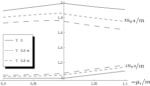
Figure 9: $m_{\pi^{0}}$ and $m_{\pi^{+}}$ as a function of the isospin chemical potential at different values of the temperature. All parameters are scaled with $m$.

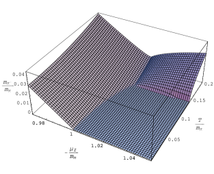
Figure 10: $m_{\pi^{-}}(T,\mu_{\mbox{\tiny I}})$. All the parameters are scaled with $m_{\pi}$

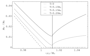
Figure 11: $m_{\pi^{-}}$ plot versus isospin chemical potential for different temperatures. All values are scaled with $m_{\pi}$. The vertical line corresponds to $\mu_{\mbox{\tiny I}}=m$.

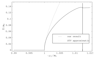
Figure 12: Phase diagram of the condensation point of temperature versus isospin chemical potential. The dashed line corresponds to the approximation made by Splittorff, Toublan and Veerbarschot Splittorff:2002xn .

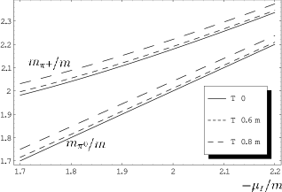
Figure 13: $m_{\pi^{0}}$ and $m_{\pi^{+}}$ as a function of high values of the isospin chemical potential at different values of temperature. All parameters are scaled with $m$

To start the discussion, we would like to mention that near the transition point, $m_{\pi^{+}}$ decreases, as in the tree-level approximation, and this behavior is enforced with temperature. In this region $m_{\pi^{0}}$ grows with both parameters (see Fig. 9).

For $m_{\pi^{-}}$, according to FIG. 10 and FIG. 11, we see that a certain critical temperature must be reached before the $\pi^{-}$ is removed from the condensed state. This is precisely the condition that determines the phase transition curve (Fig. 12). In Loewe:2002tw ; Loewe:2003dq ,we obtained the phase transition diagram in the $\mu_{\mbox{\tiny I}},T$ space, starting from the first phase by extrapolating the mass evolution $m_{\pi}(T,\mu_{\mbox{\tiny I}})$ up to the point where it vanishes. This curve has the same shape as the one shown in Barducci:2004tt (but for different values, confirming the discrepancy of about 25% the authors mentioned, obtained within a Nambu-Jona-Lasinio model analysis) and indicated previously in Son:2000xc ; Son:2000by .

Starting from the first phase, according to our previous paper Loewe:2002tw ; Loewe:2003dq , for $T<m_{\pi}$, it is possible to find at first order in $T$ an expression for the transition line $\mu_{\mbox{\tiny I}}(T)$ that coincides with the results given in EQ. (8.91) from Splittorff:2002xn . In FIG. 12, the dashed line corresponds to this approximation, valid at low temperature. However, as we said, this result gives us the transition line from the viewpoint of the first phase. If we start from the condensed phase, considering the same expansion, except that now $T<|\mu_{\mbox{\tiny I}}|$ we find that

$$T_{cr}(\mu_{\mbox{\tiny I}})\approx|\mu_{\mbox{\tiny I}}|\left(\frac{\bar{l}_{3}^{2}}{32\pi\zeta(3/2)^{2}}\right)^{1/3}$$ (59)

The reader could think from FIG.12 that the critical temperature remains constant in the second phase. However, the temperature actually rises as function of the chemical potential, as we can see from the previous equation, but very slowly, and therefore we cannot appreciate this behavior from the values shown in the figure. This growing behavior of the critical temperature, is of course consistent with general statements about phase transitions in the Ginzburg-Landau theory and it has been actually measured in the lattice for two or three color QCD. Nevertheless, if we consider the thermal corrections in the second phase, it happens that the condensation phenomenon starts to disappear for a certain value of $T>20MeV$ near the transition point, remaining a kind of superfluid phase which includes the condensed as well as the normal phase (massive pion modes).

In the high chemical potential region, as we said before, the $\pi^{-}$ pion condenses again. For $m_{\pi^{0}}$ in this region, it increases monotonically both with temperature and chemical potential. $m_{\pi^{+}}$, as the temperature and the chemical potential rise, becomes asimptotically close to $m_{\pi^{0}}$ as was expected (see FIG. 13). In contrast with the first region, the $\pi^{+}$ mass grows with temperature and a crossover occurs somewhere in the intermediate region of the chemical potential for the temperature dependence, since near the phase transition point we have $m_{\pi^{+}}(T_{1},\mu_{\mbox{\tiny I}})>m_{\pi^{+}}(T_{2},\mu_{\mbox{\tiny I}})$ and this behavior changes in the high chemical potential region in such a way that $m_{\pi^{+}}(T_{1},\mu_{\mbox{\tiny I}})<m_{\pi^{+}}(T_{2},\mu_{\mbox{\tiny I}})$.

Acknowledgements: The work of M.L. has been supported by Fondecyt (Chile) under grant No.1010976. C.V. acknowledges support from Conicyt

References

(1)
M. Loewe and C. Villavicencio,
Phys. Rev. D67, 074034 (2003), hep-ph/0212275.
(2)
M. Loewe and C. Villavicencio,
Nucl. Phys. Proc. Suppl. 121, 291 (2003).
(3)
C. A. Dominguez, M. S. Fetea, and M. Loewe,
Phys. Lett. B387, 151 (1996), hep-ph/9608396.
(4)
J. Gasser and H. Leutwyler,
Phys. Lett. B184, 83 (1987).
(5)
A. Larsen,
Z. Phys. C33, 291 (1986).
(6)
C. Contreras and M. Loewe,
Int. J. Mod. Phys. A5, 2297 (1990).
(7)
A. Barducci, R. Casalbuoni, S. De Curtis, R. Gatto, and G. Pettini,
Phys. Rev. D46, 2203 (1992).
(8)
A. Schenk,
Nucl. Phys. B363, 97 (1991).
(9)
A. Schenk,
Phys. Rev. D47, 5138 (1993).
(10)
D. Toublan,
Phys. Rev. D56, 5629 (1997), hep-ph/9706273.
(11)
J. B. Kogut, M. A. Stephanov, and D. Toublan,
Phys. Lett. B464, 183 (1999), hep-ph/9906346.
(12)
J. B. Kogut, M. A. Stephanov, D. Toublan, J. J. M. Verbaarschot, and
A. Zhitnitsky,
Nucl. Phys. B582, 477 (2000), hep-ph/0001171.
(13)
J. B. Kogut and D. Toublan,
Phys. Rev. D64, 034007 (2001), hep-ph/0103271.
(14)
D. T. Son and M. A. Stephanov,
Phys. Rev. Lett. 86, 592 (2001), hep-ph/0005225.
(15)
D. T. Son and M. A. Stephanov,
Phys. Atom. Nucl. 64, 834 (2001), hep-ph/0011365.
(16)
G. X. Peng, U. Lombardo, M. Loewe, H. C. Chiang, and P. Z. Ning,
Int. J. Mod. Phys. A18, 3151 (2003), hep-ph/0304251.
(17)
G. X. Peng, M. Loewe, U. Lombardo, and X. J. Wen,
(2003), hep-ph/0309304.
(18)
D. Toublan and J. B. Kogut,
Phys. Lett. B564, 212 (2003), hep-ph/0301183.
(19)
A. Barducci, G. Pettini, L. Ravagli, and R. Casalbuoni,
Phys. Lett. B564, 217 (2003), hep-ph/0304019.
(20)
K. Splittorff, D. Toublan, and J. J. M. Verbaarschot,
Nucl. Phys. B639, 524 (2002), hep-ph/0204076.
(21)
G. V. Dunne and S. M. Nishigaki,
Nucl. Phys. B670, 307 (2003), hep-ph/0306220.
(22)
R. F. Alvarez-Estrada and A. Gomez Nicola,
Phys. Lett. B355, 288 (1995),
Erratum: Ibid, B380:491-492, 1996.
(23)
A. Ayala, P. Amore, and A. Aranda,
Phys. Rev. C66, 045205 (2002), hep-ph/0207081.
(24)
J. B. Kogut, D. Toublan, and D. K. Sinclair,
Phys. Lett. B514, 77 (2001), hep-lat/0104010.
(25)
J. B. Kogut and D. K. Sinclair,
Phys. Rev. D66, 014508 (2002), hep-lat/0201017.
(26)
J. B. Kogut and D. K. Sinclair,
Phys. Rev. D66, 034505 (2002), hep-lat/0202028.
(27)
J. B. Kogut, D. Toublan, and D. K. Sinclair,
Nucl. Phys. B642, 181 (2002), hep-lat/0205019.
(28)
J. B. Kogut, D. Toublan, and D. K. Sinclair,
Phys. Rev. D68, 054507 (2003), hep-lat/0305003.
(29)
J. Gasser and H. Leutwyler,
Ann. Phys. 158, 142 (1984).
(30)
K. Splittorff, D. Toublan, and J. J. M. Verbaarschot,
Nucl. Phys. B620, 290 (2002), hep-ph/0108040.
(31)
M. Le Bellac,
Thermal Field Theory (Cambridge Monographs on Mathemathical
Physics, 1996).
(32)
A. Barducci, R. Casalbuoni, G. Pettini, and L. Ravagli,
Phys. Rev. D69, 096004 (2004), hep-ph/0402104.