Out-of-Equilibrium Collinear Enhanced Equilibration in the Bottom-Up Thermalization Scenario in Heavy Ion Collisions

Abstract

Experimental measurement of the elliptic flow parameter $v_{2}$ and hydrodynamic model together showed that thermalization in the central region at the Relativistic Heavy Ion Collider to be perplexingly fast. This is a mystery in itself since none of the numerical perturbative QCD models are able to achieve such a feat. By exploiting a theoretical oversight on collinear processes in an out-of-equilibrium system it is argued that, in the bottom-up thermalization scenario, equilibration can proceed at a higher rate than what is expected in the conventional perturbative QCD picture.

I Introduction

Recently measurement by STAR st1 ; st2 ; rs , PHENIX lacey and PHOBOS park collaborations of the elliptic flow parameter $v_{2}$ in the central region at the Relativistic Heavy Ion Collider (RHIC) at Brookhaven agreed with that generated from simulation using the hydrodynamic model o92 ; ksh ; khh ; hkhrv . As is well-known that hydrodynamical model required that a system to be in complete equilibrium. This implies that the central region in the collisions at RHIC achieved equilibrium within an extremely short time of around 0.6 fm/c. In case one has any doubts about this conclusion, the authors investigated an alternate scenario where the collision system was thermalized only in the transverse directions hzwo . We find that it is impossible to achieve the same $v_{2}$ results while keeping the same final transverse momentum distribution. Even trying to maintain the latter required very drastic modification to the initial conditions so that these become unrealistic. This is both good and bad news from a theoretical point of view. It is good because a fully thermalized environment at least in the central region permits a lot of simplifications in the calculation. A thermalized system is much simpler than an out-of-equilibrium system. However this is also bad news because it shows that we have not fully understood what really happens in the initial stage of the collisions. There are two reasons for that. First it was shown in mg1 ; mg2 ; mg3 that the special case of the parton cascade model kg1 ; kg2 ; pcm with only elastic collisions required either an initial parton density or the elastic cross section 15 times greater than the actual value in order to reproduce the same elliptic flow measured in the experiments. This is a huge factor, one does not expect, based on today’s knowledge, that including inelastic collisions will produce a large enough total cross section. Second it is our opinion that none of the parton based numerical models for simulating heavy ion collisions, parton cascade included, is showing such perplexingly fast thermalization kg1 ; kg2 ; pcm ; wong1 . They do show signs that the system is approaching equilibrium at a rapid pace even in the face of the longitudinal expansion, but none of these models managed to thermalize within as short an interval as 0.6 fm/c. We do not consider the results from other non-parton based models because they use other less well understood and less rigorous mechanisms such as strings, hadronic collisions etc or the combinations any of these. In any case it is hard to justify the use of any hadronic mechanisms in view of the energy density that can be reached at RHIC energies. There is one other mechanism that can be at work which is that as the system cools, the average energy of the system must come down. This will lead to an progressive increase in the strength of the interactions wong2 . This mechanism can certainly help with equilibration. However this mechanism does not come into play until at a much later stage in the collisions, well beyond the 0.6 fm/c limit imposed by the $v_{2}$ result.

To solve this very rapid equilibration problem, the first question that one has to decide is what mechanism leads to this fantastic result. Is it perturbative or nonperturbative in nature? Parton cascade model is supposed to have incorporated all known and relevant perturbative QCD effects pcm . One can easily conclude that the as-yet-unknown mechanism must be nonperturbative. Nevertheless another picture of the nuclei exists that involved viewing the initial nuclei as a frozen crystalline glass of QCD color cgc . Initial conditions produced from this model have been used to investigate and tried to answer the perturbative or nonperturbative equilibration question am . This line of investigation resulted eventually in ref. betal , this paper used a result already pointed out in wong1 which is that thermalization cannot come from leading order processes alone, higher order processes are important too. It was concluded in betal that the equilibration could proceed perturbatively. However this paper did not address how rapid a perturbative QCD based equilibration could proceed. Even if equilibration in heavy ion collisions can be achieved via perturbative QCD alone, can it be done with such phenomenal speed as revealed by the combination of elliptic flow measurements and the hydrodynamic model? There is a clear advantage of a perturbation theory based rapid equilibration as opposed to a nonperturbative one. The former is well understood theoretically and tested in experiments while the latter is less rigorous and based on a much less solid foundation. Therefore before one draws any definitive conclusion based on the results of the parton based models and gives up on perturbative QCD, another careful examination is warranted.

We will show in this paper that there is indeed a new mechanism that has been overlooked largely because of a piece of well-known knowledge that has been overly generalized and assumed to hold under all circumstances even though no careful study has been done in some situations. By this we means the cancellation of collinear divergence for a theory of massless particles which has been shown to be true in the vacuum kin ; ln and in an equilibrium system. Indeed this is true in the vacuum as total cross-sections are free of any collinear logarithms as these are cancelled between the real and virtual contributions. This is also true for a system of massless particles in equilibrium. Because of this, one tends to assume tacitly that the same will also hold in a non-equilibrium environment. This is not true. In general this cancellation between real and virtual graphs ceases to occur for a system that is not in equilibrium. One might be alarmed by this statement since there should not be any remaining divergences. This is reasonable but thanks to screening in a medium such divergences do not exist. The cancellation of collinear logarithms for a system in equilibrium is thus a double safeguard against this kind of divergences. In such a system, removing either screening or the cancellation of collinear logarithms alone does not result in any divergences. In the rest of the paper, we will show in details how there are necessarily non-cancelled collinear logarithms in an out-of-equilibrium parton plasma and how this result can be exploited to bring about a thermalization via perturbative QCD that can proceed at a higher speed than any parton models have shown thus far.

II The most relevant collision processes for equilibration

In the early stage of the system, the plasma is gluon dominated because of the small-x growth in the gluon distribution in the nucleons and also because of the stronger gluon-gluon interactions than that of gluon-(anti)quark or (anti)quark-(anti)quark. Therefore for our present attempt at explaining the very fast thermalization seen in experiments, one only has to consider a pure gluon plasma. In general there are many possible interactions even only among gluons. Not all of them are useful for the purpose of equilibration. We will group the different contributions below and discuss the importance and relevance of them with regard to thermalization.

II.1 $2\longleftrightarrow 2$ scattering

• Small angle collision: At the leading order, it is the simple 2-to-2 gluon-gluon scattering. It is well known that this process is dominated by small angle scatterings because of the familiar Coulomb exchange divergence at small momentum transfer. Although the probability of this process is large, the outgoing momenta are not that different from the incoming ones since they are only rotated somewhat in momentum space from the incoming momenta. Thus this normally dominant process is in fact terribly inefficient at driving the system towards equilibration.

• Large angle collision: At the same order, there is the remaining large angle scattering process. The outgoing momenta are necessarily very different from the incoming ones therefore large angle scatterings are much better at redistributing momenta which is the essence of what thermalization is about. The drawback of this process is that the probability is not nearly as large as the small angle collisions. There will be an occasional large angle collision amongst the much more frequent small angle collisions.

At this level of the basic 2-to-2 scattering, the possibility for the driving force behind the equilibration process is restricted between a probable but inefficient small angle scatterings and a less probable but more efficient large angle collisions. This is not very promising. Indeed as have been pointed out in the second reference of wong1 , the elastic scattering process is not the main driving force for equilibration. This is because in that numerical study, the entropy generation rate from 2-to-2 scatterings is not only comparable but sometimes even subdominant to that of the 2-to-3 gluon processes. This point of view is reinforced in a later paper betal . Therefore higher order processes must be considered. The key question is which higher processes?

II.2 $2\longleftrightarrow 3$ scattering

We now attempt to identify what processes at this order are most relevant and most important for thermalization.

• Small angle collisions with a small angle gluon radiation/absorption: At order $\alpha_{s}^{3}$ there is the possibility of a gluon emission on top of the main scattering. Since the emitted gluon can be of any magnitude limited only by energy-momentum conservation, this is a much more flexible process for achieving equilibration. However flexibility is not the only factor that one has to consider. In this case, all the momenta are aligned around the directions of the two incoming momenta. So there is still no significant momentum transfer here. Besides there is the extra power of $\alpha_{s}$ that reduces the effectiveness of this contribution. The same applies to the small angle absorption.

• Small angle collisions with a large angle gluon radiation/absorption: This type of contributions come in two different forms. One can be reclassified as large angle collisions with a small angle emission or absorption to be discussed below. Those contributions that cannot be reclassified are as before down by a power of $\alpha_{s}$ although in view of the large angle gluon emission and the small angle scattering, they are potentially useful for achieving equilibration.

• Large angle collisions with a small angle gluon radiation/absorption: Again large angle collisions are important for sizable momentum rearrangement as already mentioned, what is more important is the well-known fact that small angle gluon emission or absorption accompanying a hard collision can give rise to a large collinear logarithm in the probability provided that the collision is sufficently hard. In the medium this is determined by both the hardness of the collisions and the medium screening, this will be seen in later sections. These kind of large logarithms can compensate for the small power of $\alpha_{s}$ that comes with the gluon emission or absorption. Thus the contribution from this type of processes is comparable in size to that from the leading order.

• Large angle collisions with a large angle gluon radiation/absorption: Large angle processes sadly do not receive any collinear logarithmic compensation of the small coupling. Processes discussed in (iii) are definitely more important for this reason.

II.3 Higher order processes

Going to even higher orders, one can have various mixtures of large and small angle processes given that the possibilities are nearly endless as one goes to higher and higher order. Afterall we are using perturbative QCD, higher processes are in general less important. From the above discussion, we have ascertained that large angle processes are useful for equilibration because of their ability to rearrange the momentum distribution. However they are weighed down by the coupling and have no singularity to enhance the frequency of their occurrence. It is certain therefore that there cannot be too many large angle subprocesses in any given scattering and there cannot be none either. The simplest way to proceed is to combine both large and small angle processes. Since there must be at least one large angle process and the coupling associated with small angle subprocesses can only be compensated by a large collinear logarithm if there is a hard scattering and/or small screening, it is logical that for contribution at any order to have one hard collision to be accompanied by all sorts of collinear subprocesses. These type of contributions are now comparable in size to that of the leading order 2-to-2 scattering. These are the processes that we considered to be most important for equilibration and we will concentrate on these contributions and consider them further up to order $\alpha_{s}^{3}$ in the rest of this paper. Note that we are not relying solely on the momentum rearranging power of the large angle collisions. They serves mainly to direct and guide where the remaining gluon radiations will populate the momentum space. It is these radiations that actually help to bring about thermalization of the system.. In a way we are arguing for using multi-gluon processes to achieve rapid thermalization not dissimilar to what was done in shx for achieving chemical equilibration. Whereas in shx they included mostly every $ng\leftrightarrow mg$ process indiscriminately, we consider only what in our opinion the most important processes for thermalization here.

Notwithstanding of what was mentioned in the introduction, any alert readers will rightly object that one cannot use collinear processes in this way because of the cancellation between the real and virtual contribution kin . This is true only if there is a sum over degenerate states ln . The equilibration of a gluon plasma, and in fact for other many-body systems as well, is not at all inclusive because momentum regions are separate from one another. The processes cannot be any more exclusive than this but it is usual to study interactions and momentum states collectively, in which case one has indeed to consider this cancellation. As mentioned in the introduction and we will see below, this cancellation does not hold in an out-of-equilibrium system wip . But there is no need to worry about any divergence because where there is screening, the interaction probability is always finite.

III The leading and next-to-leading order collision processes

An out of equilibrium system is necessarily time dependent, there must be a transport equation to study such a system. The simplest and possibly the most used is the Bolzmann equation

$$p^{\mu}\frac{\partial f(x,p)}{\partial x^{\mu}}=C(x,p)\,,$$ (1)

On the right hand side are the collision terms which contain all the microscopic interactions. Since they are the main reason that a many-body system can equilibrate, we will spend the rest of the article studying these. As is commonplace in perturbative QCD, the collinear gluons are either on-shell or are nearly on-shell so that only the transverse degrees of freedom are relevant. Therefore a physical gauge such as the lightcone gauge will be used throughout.

III.1 The leading gluon-gluon collision process

Figure 1: The basic scattering of gluon 1 with gluon 2 resulting in gluon 3 and 4. Likewise one can view this equally as gluon 3 scatters with gluon 4 giving gluon 1 and 2.

The basic gluon-gluon collision is well-known. Graphically we represent it by Fig. 1. The collision term is

$$C_{12\leftrightarrow 34}(p_{1}) = -\int[dp_{2}][dp_{3}][dp_{4}]D_{12,34}\,\frac{1}{2!}\overline{|{\cal M}_{12\rightarrow 34}|^{2}}$$ (2)

$$\hskip 28.45274pt\times\bigl{[}f_{1}f_{2}(1{+}f_{3})(1{+}f_{4})-(1{+}f_{1})(1{+}f_{2})f_{3}f_{4}\bigr{]}\,.$$

Here $f_{j}=f(p_{j})$, $[dp]$ represents the invariant momentum-space integration measure for an on-shell gluon with momentum $p$,

$$[dp]={d^{4}p\over(2\pi)^{3}}\,\theta(p^{0})\,\delta(p^{2})=\frac{d^{3}p}{(2\pi)^{3}2E_{p}}\,,$$ (3)

with $E_{p}=|\bm{p}|$ for massless gluons, and $D_{12,34}$ is the energy-momentum conserving $\delta$-function

$$D_{12,34}=(2\pi)^{4}\delta^{(4)}(p_{1}+p_{2}-p_{3}-p_{4})\;.$$ (4)

The square of the matrix element is given by ckr

$$\overline{|{\cal M}_{12\rightarrow 34}|^{2}}=\frac{1}{\nu_{g}}\sum|{\cal M}_{12\rightarrow 34}|^{2}=72\,\nu_{g}\pi^{2}\alpha_{s}^{2}(Q^{2})\Big{(}3-\frac{ut}{s^{2}}-\frac{us}{t^{2}}-\frac{st}{u^{2}}\Big{)}$$ (5)

where the sum is over spins and colors, $s=(p_{1}{+}p_{2})^{2}$, $t=(p_{1}{-}p_{3})^{2}$, and $u=(p_{1}{-}p_{4})^{2}=-s-t$. For the scale of the running coupling constant $\alpha_{s}(Q^{2})$ we can take $Q^{2}=\min(|s|,|t|,|u|)$. At momentum scales where there are three active quark flavors, it can be parametrized as

$$\alpha_{s}(Q^{2})=\frac{4\pi}{\beta_{0}\ln(Q^{2}/\Lambda_{(3)}^{2})}$$ (6)

where $\Lambda_{(3)}=0.246$ GeV and $\beta_{0}=9$. We will assume that $Q$ is significantly larger than the scale $\Lambda$ associated with non-perturbative QCD effects.

III.2 The gluon-gluon collision with collinear emission or absorption

For 5-gluon processes there are two distinct contributions to the collision terms:

$$C_{12\leftrightarrow 345}(p_{1}) = -\frac{1}{3!}\int[dp_{2}]d\Phi_{345}D_{12,345}\,\overline{|{\cal M}_{12\rightarrow 345}|^{2}}$$ (7)

$$\hskip 28.45274pt\times\bigl{[}f_{1}f_{2}(1{+}f_{3})(1{+}f_{4})(1{+}f_{5})-(1{+}f_{1})(1{+}f_{2})f_{3}f_{4}f_{5}\bigr{]},$$

and

$$C_{123\leftrightarrow 45}(p_{1}) = -\frac{1}{2!2!}\int d\Phi_{23}d\Phi_{45}D_{123,45}\,\overline{|{\cal M}_{123\rightarrow 45}|^{2}}$$ (8)

$$\hskip 28.45274pt\times\bigl{[}f_{1}f_{2}f_{3}(1{+}f_{4})(1{+}f_{5})-(1{+}f_{1})(1{+}f_{2})(1{+}f_{3})f_{4}f_{5}\bigr{]}.$$

We have introduced a compact notation for the multiparticle phase space:

$$\int d\Phi_{12\dots m}=[dp_{1}][dp_{2}]\cdots[dp_{m}]\,.$$ (9)

Every such factor is accompanied by a symmetry factor $1/m!$. The energy-momentum conserving delta functions $D_{12,345}$ and $D_{123,45}$ are the obvious generalizations of Eq. (4).

Suppose the 5-gluon processes $12\leftrightarrow 345$ in Eq. (7) and $123\leftrightarrow 45$ in Eq. (8) consist of a hard-scattering collision involving four gluons. Then two of the incoming or outgoing gluons can be hard but collinear. If the two gluons ($i$,$j$) are both in the initial or both in the final state, collinear means that their invariant mass $s_{ij}=(p_{i}+p_{j})^{2}$ is significantly less than $Q^{2}$, where $Q$ is the momentum scale of the hard scattering. If one is in the initial state and one is in the final state, collinear means that their momentum transfer $|t_{ij}|=-(p_{i}-p_{j})^{2}$ is likewise significantly less than $Q^{2}$. For the process $12\leftrightarrow 345$, there are nine possibilities for the collinear pair of gluons ($i$,$j$). By exploiting the Bose symmetry, we can take the collinear pair to be (1,5), (2,5) or (4,5). For the process $123\rightarrow 45$, there are again nine possibilities for the collinear pair. Again by exploiting the Bose symmetry, we can take the collinear pair to be (1,3), (2,3) or (4,3). For each of the possible collinear pairs, we wish to calculate the contribution to the collision terms $C(p)$ from the collinear region of phase space. We will label the contribution in which gluons $i$ and $j$ are collinear by $i\!\parallel\!j$.

III.2.1 Both collinear gluons in the initial or final state

We first consider the case in which the collinear gluons are either both in the initial state or else both in the final state and neither is the external gluon 1 (of course there is nothing special about gluon 1 except its momentum has been chosen to be the argument of the collision terms). We begin by considering the scattering process $12\rightarrow 3ij$ in which the two collinear gluons are both in the final state with momenta $p_{i}$ and $p_{j}$. The matrix element ${\cal M}_{12\rightarrow 3ij}$ has a pole in the invariant mass $s_{ij}$. In the collinear region in which $s_{ij}\ll Q^{2}$, we can interpret the process as proceeding through a hard-scattering $12\rightarrow 34^{*}$ that creates a virtual gluon $4^{*}$ with momentum $p_{4^{*}}=p_{i}+p_{j}$ followed by the decay of the virtual gluon into the two collinear gluons $i$ and $j$.

It is convenient to introduce light-cone variables defined by the direction of the 3-momentum ${p}_{4^{*}}={p}_{i}+{p}_{j}$ in the rest frame of the plasma. The momenta of the collinear gluons and the virtual gluons can be written as

$$p_{i} = \Big{(}zp^{+}_{4},\frac{{p}_{\perp}^{2}}{zp^{+}_{4}},{p}_{\perp}\Big{)}$$ (10)

$$p_{j} = \Big{(}(1-z)p^{+}_{4},\frac{{p}_{\perp}^{2}}{(1-z)p^{+}_{4}},-{p}_{\perp}\Big{)}$$ (11)

$$p_{4^{*}} = \Big{(}p^{+}_{4},\frac{s_{ij}}{p^{+}_{4}},\mathbf{0_{\perp}}\Big{)}$$ (12)

where $p^{+}_{4}$ is the total light-cone momentum of the collinear gluons. The variable $z$ is the fraction of that light-cone momentum that comes from gluon $i$. The light-cone energies are determined by the mass-shell constraints $p_{i}^{2}=p_{j}^{2}=0$. The invariant mass $s_{ij}$ of the virtual gluon is determined by conservation of light-cone energy:

$$s_{ij}=\frac{{p}_{\perp}^{2}}{z}+\frac{{p}_{\perp}^{2}}{1-z}=\frac{{p}_{\perp}^{2}}{z(1-z)}\;.$$ (13)

The phase space integral in light-cone variables is

$$[dp]=\frac{dp^{+}}{4\pi p^{+}}\frac{d^{2}{p}_{\perp}}{(2\pi)^{2}}=\frac{dz}{4\pi z}\frac{d^{2}{p}_{\perp}}{(2\pi)^{2}}\;,$$ (14)

the latter form applies when $p$ is the momentum of the daughter of a parent gluon from which a fraction $z$ of its light-cone momentum has been inherited. We define the momentum $p_{4}$ of an on-shell gluon that has the same light-cone momentum as the virtual gluon $4^{*}$ but whose light-cone energy is determined by the mass shell constraint $p^{2}_{4}=0$:

$$p_{4}=\Big{(}p^{+}_{4},0,\mathbf{0_{\perp}}\Big{)}\;.$$ (15)

We proceed to make approximations to the collision integral Eq. (7) (with 45 replaced by $ij$) that are valid in the collinear region. In the amplitude for $12\rightarrow 34^{*}$, we can replace the momentum $p_{4^{*}}$ of the virtual gluon by the quasi on-shell momentum $p_{4}$, since the invariant mass $s_{ij}$ is small compared to the hard-scattering scale. In the amplitude for the decay $4^{*}\rightarrow ij$, we keep only the most singular term which will give rise to a logarithm of $Q$ after integrating over phase space. The square of the matrix element, averaged over initial spins and colors and summed over those of the final state, then reduces to

$$\sum|{\cal M}_{12\rightarrow 3ij}|^{2}\simeq\frac{8\pi\alpha_{s}(s_{ij})}{s_{ij}}P_{gg}(z)\sum|{\cal M}_{12\rightarrow 34}|^{2}$$ (16)

where $P_{gg}(z)$ is the unregularized $g\rightarrow gg$ splitting function

$$P_{gg}(z)=2\,C_{A}\Big{(}\frac{1-z}{z}+\frac{z}{1-z}+z(1-z)\Big{)}$$ (17)

where $C_{A}=3$ is a color factor. The scale of the explicit factor of $\alpha_{s}$ in Eq. (16) is $\sqrt{s_{ij}}$. We can make similar approximations in the phase space integrals. We first express the phase space for gluons $i$ and $j$ in an iterated form involving an integral over the momentum of the virtual gluon $4^{*}$

$$\int[dp_{i}][dp_{j}]D_{12,3ij}=\int\frac{ds_{ij}}{2\pi}[dp_{4^{*}}]D_{12,34^{*}}\int[dp_{i}][dp_{j}]D_{4^{*},ij}\;.$$ (18)

In the collinear region, we can approximate $p_{4^{*}}$ by $p_{4}$ in the measure $[dp_{4^{*}}]$ and in the delta function $D_{12\rightarrow 34^{*}}$. The expression for the phase space integral Eq. (18) then reduces to

$$\int[dp_{i}][dp_{j}]D_{12,3ij}\simeq\int[dp_{4}]D_{12,34}\frac{dz\;d{p}_{\perp}^{2}}{16\pi^{2}z(1-z)}=\int[dp_{4}]D_{12,34}\frac{dz\;ds_{ij}}{16\pi^{2}}\;.$$ (19)

Combining the approximations Eqs. (16) and (19) and using Eq. (13), we get

$$\int d\Phi_{3ij}D_{12,3ij}\sum|{\cal M}_{12\rightarrow 3ij}|^{2}\simeq\int d\Phi_{34}D_{12,34}\sum|{\cal M}_{12\rightarrow 34}|^{2}\times\int\frac{dz\;ds_{ij}}{s_{ij}}\frac{\alpha_{s}(s_{ij})}{2\pi}P_{gg}(z)\;.$$ (20)

Figure 2: An example of the 2-to-3 or 3-to-2 gluon process when gluon $4\!\!\parallel\!\!5$.

Our final step is to use a collinear approximation in the distribution functions $f_{i}$ and $f_{j}$ for the gluons. Since their momenta have components of order $Q$, we can neglect their transverse momenta and approximate them by $f_{4}(z)$ and $f_{4}(1-z)$, where

$$f_{i}(z)\equiv f(zp_{i})\;.$$ (21)

Thus our final expression for the contribution to the collision integral Eq. (7) from the region in which gluons 4 and 5 are collinear is

$$C^{4\parallel 5}_{12\leftrightarrow 345}(p_{1}) \simeq -\frac{1}{\nu_{g}}\int[dp_{2}]d\Phi_{34}D_{12,34}\frac{1}{3!}\sum|{\cal M}_{12\rightarrow 34}|^{2}\times\int dz\frac{ds_{45}}{s_{45}}\frac{\alpha_{s}(s_{45})}{2\pi}P_{gg}(z)$$

$$\times\Big{[}f_{1}f_{2}(1+f_{3})(1+f_{4}(z))(1+f_{4}(1-z))-(1+f_{1})(1+f_{2})f_{3}f_{4}(z)f_{4}(1-z)\Big{]}\;.$$

Depicted in Fig. 2 is the feynman graph for this contribution when $4\!\!\parallel\!\!5$. The contribution from the collinear regions $3\!\!\parallel\!\!4$ and $3\!\!\parallel\!\!5$ are given by exactly the same expression after appropriate relabelling of the momenta.

The contribution to the collision integral Eq. (8) from the collinear region $2\!\!\parallel\!\!3$ is given by a similar expression. After relabelling the dummy momentum variables $45\rightarrow 34$, it can be written as

$$C^{2\parallel 3}_{123\leftrightarrow 45}(p_{1}) \simeq -\frac{1}{\nu_{g}}\int[dp_{2}]d\Phi_{34}D_{12,34}\frac{1}{2!2!}\sum|{\cal M}_{12\rightarrow 34}|^{2}\times\int dz\frac{ds_{23}}{s_{23}}\frac{\alpha_{s}(s_{23})}{2\pi}P_{gg}(z)$$

$$\times \!\Big{[}f_{1}f_{2}(z)f_{2}(1-z)(1+f_{3})(1+f_{4})-(1+f_{1})(1+f_{2}(z))(1+f_{2}(1-z))f_{3}f_{4}\Big{]}\;.$$

In both Eqs. (LABEL:eq:bif-23) and (LABEL:eq:bif-32), the ranges of the integrals over $z$ and $s_{ij}$ have not been specified. The ranges in which our collinear approximation remain valid will be specified later after a discussion of hard-thermal loop corrections.

III.2.2 One collinear gluon in the initial and the other in the final state

We next consider the case in which one of the collinear gluons is in the initial state and one is in the final state and neither is the external gluon 1. We begin by considering the scattering process $1i\rightarrow 34j$, where gluons $i$ and $j$ are collinear. The matrix element ${\cal M}_{1i\rightarrow 34j}$ has a pole in the variable $t_{ij}=(p_{i}-p_{j})^{2}$. In the collinear region $|t_{ij}|\gg Q^{2}$, we can interpret the process as the splitting of gluon $i$ into a real gluon $j$ and a virtual gluon $2^{*}$ with momentum $p_{2^{*}}=p_{i}-p_{j}$, followed by the hard scattering $12^{*}\rightarrow 34$.

We introduce light-cone variables defined by the direction of ${p}_{i}$ in the rest frame of the plasma. The momenta of the collinear gluons and the virtual gluon $2^{*}$ can be written as

$$p_{i} = \Big{(}\frac{p^{+}_{2}}{x},0,\mathbf{0_{\perp}}\Big{)}$$ (24)

$$p_{j} = \Big{(}\frac{(1-x)p^{+}_{2}}{x},\frac{x{p}_{\perp}^{2}}{(1-x)p^{+}_{2}},-{p}_{\perp}\Big{)}$$ (25)

$$p_{2^{*}} = \Big{(}p^{+}_{2},\frac{t_{ij}+{p}_{\perp}^{2}}{p^{+}_{2}},{p}_{\perp}\Big{)}$$ (26)

where $p^{+}_{2}$ is the difference between the light-cone momenta of the collinear gluons. The variable $x$ is the fraction of the light-cone momentum of gluon $i$ that is carried by the virtual gluon $2^{*}$. The light-cone energies of $i$ and $j$ are determined by the mass shell constraints $p^{2}_{i}=p^{2}_{j}=0$. The invariant mass of the virtual gluon is determined by the conservation of light-cone energy

$$t_{ij}=-\frac{{p}_{\perp}^{2}}{1-x}\;.$$ (27)

We define the momentum $p_{2}$ of an on-shell gluon that has the same light-cone momentum as the virtual gluon $2^{*}$ and the same transverse momentum as gluon $i$:

$$p_{2}=(p^{+}_{2},0,\mathbf{0_{\perp}})\;.$$ (28)

Figure 3: An example of the 2-to-3 or 3-to-2 gluon process when gluon $2\!\!\parallel\!\!5$.

We proceed to make approximations to the collision integral Eq. (7) (with the pair (2,5) replaced by ($i$,$j$)) that are valid in the collinear region Fig. 3. The square of the matrix element can be approximated as follows

$$\sum|{\cal M}_{1i\rightarrow 34j}|^{2}\simeq\frac{8\pi\alpha_{s}(|t_{ij}|)}{|t_{ij}|}P_{gg}(x)\sum|{\cal M}_{12\rightarrow 34}|^{2}$$ (29)

where the scale of the explicit factor of $\alpha_{s}$ is $\sqrt{-t_{ij}}$. The phase space integral can be approximated by

$$\int[dp_{i}][dp_{j}]D_{1i,34j}\simeq\int[dp_{2}]D_{12,34}\frac{dx\;d{p}_{\perp}^{2}}{16\pi^{2}(1-x)}=\int[dp_{2}]D_{12,34}\frac{dx\;d(-t_{ij})}{16\pi^{2}}\;.$$ (30)

The distribution functions $f_{i}$ and $f_{j}$ can be approximated by $f_{2}({1\over x})$ and $f_{2}({1-x\over x})$, respectively. Combining all these approximations, the final expression for the contribution to the collision integral Eq. (7) from the region $2\!\!\parallel\!\!5$ is

$$C^{2\parallel 5}_{12\leftrightarrow 345}(p_{1}) \simeq -\frac{1}{\nu_{g}}\int[dp_{2}]d\Phi_{34}D_{12,34}\frac{1}{3!}\sum|{\cal M}_{12\rightarrow 34}|^{2}\times\int dx\frac{dt_{25}}{t_{25}}\frac{\alpha_{s}(|t_{25}|)}{2\pi}P_{gg}(x)$$

$$\times\Big{[}f_{1}f_{2}(\mbox{$1\over x$})(1+f_{3})(1+f_{4})(1+f_{2}(\mbox{$1-x\over x$}))-(1+f_{1})(1+f_{2}(\mbox{$1\over x$}))f_{3}f_{4}f_{2}(\mbox{$1-x\over x$})\Big{]}\;.$$

The identical expression is obtained for $2\!\!\parallel\!\!3$ or $2\!\!\parallel\!\!4$.

We can derive a similar expression for the contribution to the collision integral Eq. (8) from regions in which one of the collinear gluon is in the initial state, the other is in the final state, and neither one is $p_{1}$. The contribution from the region $3\!\!\parallel\!\!5$ can be written as after relabelling of momenta

$$C^{3\parallel 5}_{123\leftrightarrow 45}(p_{1}) \simeq -\frac{1}{\nu_{g}}\int[dp_{2}]d\Phi_{34}D_{12,34}\frac{1}{2!2!}\sum|{\cal M}_{12\rightarrow 34}|^{2}\times\int dx\frac{dt_{35}}{t_{35}}\frac{\alpha_{s}(|t_{35}|)}{2\pi}P_{gg}(x)$$

$$\times\Big{[}f_{1}f_{2}(1+f_{3})f_{4}(\mbox{$1-x\over x$})(1+f_{4}(\mbox{$1\over x$}))-(1+f_{1})(1+f_{2})f_{3}(1+f_{4}(\mbox{$1-x\over x$}))f_{4}(\mbox{$1\over x$})\Big{]}\;.$$

An identical expression is obtained, after relabelling, for the regions $2\!\!\parallel\!\!4$, $2\!\!\parallel\!\!5$, and $3\!\!\parallel\!\!4$. In Eqs. (LABEL:eq:oif-23) and (LABEL:eq:oif-32), the ranges of $x$ and $t_{ij}$ in which our collinear approximations remain valid will be specified later after a discussion of hard-thermal-loop corrections.

III.3 Hard-thermal loop corrections

One important class of higher order corrections to the 4-gluon collision integral $C_{12\rightarrow 34}(p_{1})$ is hard-thermal-loop (HTL) corrections to the propagators of the four hard scattered gluons bp1 ; bp2 . These corrections arise from hard gluons in the medium that interact with one of the hard-scattered gluons but are then scattered back into their original momentum state. These forward scattering contributions must be added coherently over the distribution of hard gluons in the medium. The effect of these HTL corrections on transverse gluons with momenta near the light cone is very simple. They become quasi-particles with a mass $m_{t}$ given by

$$m^{2}_{t}=\frac{24\alpha_{s}(\mu^{2})}{\pi}\int^{\infty}_{0}dppf(p)$$ (33)

where $f(p)$ is the distribution of hard gluons in the medium. An appropriate choice for the scale $\mu$ of $\alpha_{s}$ is the momentum scale that dominates the integral. As an estimate for the scale, we will use

$$\mu^{2}=\frac{\int^{\infty}_{0}dpp^{3}f(p)}{\int^{\infty}_{0}dppf(p)}\;.$$ (34)

In the case of the equilibrium Bose-Einstein distribution, this description gives $\mu=\sqrt{2/5}\pi T$. We will usually refer to the transverse gluon quasi-particle simply as gluons and to the mass given by Eq. (34) as the transverse mass. The transverse mass is related to the Debye screening mass $m_{D}$ simply by $m_{t}=m_{D}/\sqrt{2}$ wel . This relation arises from the structure of HTL corrections to the gluon propagator which are strongly constrained by gauge invariance.

The HTL corrections will have particularly important effects in the regions of phase space where gluons become collinear. In particular, they provide infrared cutoff on the integrals over the momentum fraction and invariant masses that appear in the collinear contributions to the collision integrals. We will use the HTL corrections to estimate the boundaries of the integration regions where our collinear approximations remain valid.

We first consider the integral over $z$ and $s_{45}$ in the $4\!\!\parallel\!\!5$ contribution to the collision integral $C_{12\rightarrow 345}$ which is given in Eq. (LABEL:eq:bif-23). One effect of the HTL corrections is to replace the propagator $1/s$ of the virtual gluon by $1/(s-m_{t}^{2})$. Another effect is to change the mass-shell constraints on the collinear gluons to $p^{2}_{4}=p^{2}_{5}=m_{t}^{2}$. This changes the expression Eq. (13) for the invariant mass of the virtual gluon to

$$s_{45}=\frac{m_{t}^{2}+{p}_{\perp}^{2}}{z(1-z)}\;.$$ (35)

For fixed $z$, the lower limit on $s_{45}$ occurs at ${p}_{\perp}=0$:

$$s_{\min}=\frac{m_{t}^{2}}{z(1-z)}\;.$$ (36)

The upper limit on $s$ is set by the scale $Q^{2}$ of the hard scattering. We choose to write it as

$$s_{\max}=c^{2}Q^{2}+m_{t}^{2}$$ (37)

where $c$ is a constant near 1. The change from varying $c$ by a factor of 2 should be included in the theoretical error. We will take the virtuality $s_{45}-m_{t}^{2}$ of the virtual gluon to also provide the scale of the factor $\alpha_{s}$ in the collinear correction factors. The integral over $s_{45}$ can then be evaluated analytically

$$\int^{s_{\max}}_{s_{\min}}\frac{ds}{s-m_{t}^{2}}\frac{\alpha_{s}(s-m_{t}^{2})}{2\pi}=\frac{2}{\beta_{0}}\ln\left(\frac{\ln\Big{(}c^{2}Q^{2}/\Lambda^{2}\Big{)}}{\ln\Big{(}(1-z+z^{2})m_{t}^{2}/z(1-z)\Lambda^{2}\Big{)}}\right)\;.$$ (38)

The condition $s_{max}>s_{min}$ constrains the integration region for $z$ to the range $z_{\max}>z>z_{\min}$, where

$$z_{\max} = \textstyle{\frac{1}{2}}\Big{(}1+\sqrt{1-4m_{t}^{2}/(c^{2}Q^{2}+m^{2}_{t})}\Big{)}$$ (39)

$$z_{\min} = \textstyle{\frac{1}{2}}\Big{(}1-\sqrt{1-4m_{t}^{2}/(c^{2}Q^{2}+m^{2}_{t})}\Big{)}\;.$$ (40)

The condition $z_{\max}>z_{\min}$ also imposes a lower bound on $Q^{2}$:

$$Q^{2}>\frac{3}{c^{2}}m^{2}_{t}\;.$$ (41)

We next consider the integral over $x$ and $t_{25}$ in the $2\!\!\parallel\!\!5$ contribution to the collision integral $C_{12\rightarrow 345}$, which is given in Eq. (LABEL:eq:oif-23). The HTL corrections replace the propagator $1/t_{25}$ of the the virtual gluon by $1/(t_{25}-m_{t}^{2})$. They also change the mass shell constraint to $p^{2}_{2}=p^{2}_{5}=m_{t}^{2}$. The resulting expression Eq. (27) for the invariant mass of the virtual gluon is replaced by

$$t_{25}=-\frac{m_{t}^{2}+{p}_{\perp}^{2}}{1-x}\;.$$ (42)

For fixed $x$, the lower limit on $-t_{25}$ occurs at ${p}_{\perp}=0$:

$$-t_{\min}=\frac{m_{t}^{2}}{1-x}\;,$$ (43)

the upper limit on $-t_{45}$ is set by the scale $Q$ of the hard scattering. We choose to write it as

$$-t_{\max}=c^{2}Q^{2}-m_{t}^{2}$$ (44)

where $c$ is again a constant near 1. The change from varying $c$ by a factor of 2 should be included in the theoretical error. We will take the virtuality $-t_{25}+m_{t}^{2}$ of the virtual gluon to also be the scale of $\alpha_{s}$ in the collinear correction factor. The integral over $t_{25}$ can then be evaluated analytically

$$\int^{-t_{\max}}_{-t_{\min}}\frac{d(-t)}{-t+m_{t}^{2}}\frac{\alpha_{s}(-t+m_{t}^{2})}{2\pi}=\frac{2}{\beta_{0}}\ln\left(\frac{\ln\Big{(}c^{2}Q^{2}/\Lambda^{2}\Big{)}}{\ln\Big{(}(2-x)m_{t}^{2}/(1-x)\Lambda^{2}\Big{)}}\right)\;.$$ (45)

The condition $-t_{\max}>-t_{\min}$ constrains the integration range for $x$ to the region $x<x_{\max}$, where

$${x_{\max}}=1-\frac{m_{t}^{2}}{c^{2}Q^{2}}\;.$$ (46)

For the lower limit, we will set

$${x_{\min}}=\frac{m_{t}^{2}}{c^{2}Q^{2}}\;.$$ (47)

The condition $x_{\max}>0$ imposes a lower bound on $Q^{2}$

$$Q^{2}>\frac{1}{c^{2}}m_{t}^{2}\;.$$ (48)

Note that in the limit where $Q^{2}/m_{t}^{2}\gg 1$, there is little distinction between the different limits since ${z_{\max}}\simeq{x_{\max}}$ and ${z_{\min}}\simeq{x_{\min}}$.

III.4 The collinear virtual contributions at the next-to-leading order

We have not considered virtual corrections to the basic hard scattering discussed in Sec. III. These are of the same order in $\alpha_{s}$ as the 5-gluon processes. In the collinear limit, these corrections can be written in a compact way. To see this, recall that in the vacuum theory if one starts out with a virtual gluon, it has a chance of splitting into two gluons with momentum fractions $z$ and $1-z$. The associated variation in the probability density is ap

$${\cal P}_{gg}+d{\cal P}_{gg}=\delta(1-z)+\frac{\alpha_{s}}{2\pi}P^{+}_{gg}(z)ds$$ (49)

while the gluon reduces the square of its invariant mass from $s$ to a value between $s$ and $s-ds$ for a timelike branching. For spacelike branching, one substitutes $dt$ for $ds$ and $t$ is changed to a value between $t$ and $t+dt$. $P^{+}_{gg}(z)$ is the usual kernel of the Dokshitzer-Gribov-Lipatov-Altarelli-Parisi (DGLAP) equation ap ; gl ; dsz and it carries also a $\delta(1-z)$ function part. It is the ‘plus’ distribution regularized gluon splitting function ap ; esw . Since momentum is always conserved, the total momentum must always be equal to that of the original virtual gluon independent of whether splitting occurred, then $P^{+}_{gg}(z)$ must satisfy the identity (in the absence of $q$ and $\bar{q}$)

$$\int^{1}_{0}dzzP^{+}_{gg}(z)=0$$ (50)

or if we write out $P^{+}_{gg}(z)$ separately the parts with and without the $\delta(1-z)$ function

$$P^{+}_{gg}(z)=P_{gg}(z)|_{+}+{\cal C}_{T=0}\;\delta(1-z)\;,$$ (51)

where ${\cal C}_{T=0}$ is the constant in front of the $\delta$-function part of $P^{+}_{gg}(z)$, momentum conservation gives

$$\int^{1}_{0}dz\Big{\{}zP_{gg}(z)|_{+}+{\cal C}_{T=0}\;\delta(1-z)\Big{\}}=0\;.$$ (52)

The $\delta$-function part has its origin from the virtual correction to the splitting in the collinear limit. $P_{gg}(z)|_{+}$ is the same as our $P_{gg}(z)$ defined in Eq. (17) except the $1/(1-z)$ part has been regularized by the ‘plus’-distribution prescription and so is replaced by $1/(1-z)_{+}$. One can therefore write in a compact way the correction as

$${\cal C}_{T=0}=-\int^{1}_{0}dzzP_{gg}(z)|_{+}=-\frac{1}{2}\int^{1}_{0}dzP_{gg}(z)|_{+}\;.$$ (53)

This is a clever way to deduce the virtual correction from momentum conservation ap ; esw . The last expression on the right is obtained by using the property $P_{gg}(z)=P_{gg}(1-z)$ which follows also from the fact that in every branching two gluons are created for every one that gets destroyed.

For gluon splitting in a medium because of the accompanying particle distributions, the virtual corrections cannot be deduced so simply especially when the system is out-of-equilibrium. However since the basic gluon splitting remains the same, one can reasonably expect that only the integrand of Eq. (53) will be modified by some factor involving the particle distributions of particle participating in the splitting. That is we expect

$${\cal C}_{T}=-\frac{1}{2}\int^{1}_{0}dzP_{gg}(z)|_{+}H(f,z)\;,$$ (54)

where $H$ is a function of the particle distributions and the momentum fraction $z$, which will be seen presently.

Because of the medium as discussed in Sec. III.3, HTL corrections naturally establish limits on the $z$ integration within which the collinear approximation holds. These limits suffice as a regularization, we need not use the plus-distribution prescription. As a result the splitting function will always be written as $P_{gg}(z)$ from now on.

III.4.1 Type I: virtual correction with vacuum contribution

Figure 4: The self-energy insertion that gives the relevant medium virtual contributions.

We divide the virtual corrections into two types, one that has a contribution in the vacuum and the other has not. Bearing in mind that for every real process beyond the leading order, there is a virtual contribution that can be considered as its partner. They are related simply by originating from two different cuts of the same diagram kin . For this reason the pair of real and virtual contribution are closely related especially in the collinear limit. This facts allow them to be derived with some ease. The complete correction is a medium self-energy insertion shown in Fig. 4 but only the type I part of this will be discussed in this section.

Figure 5: This figure shows the type I virtual correction on gluon 4 given by the expression in Eq. (LABEL:eq:v1-4-2).

We start with the contribution that has a correction on gluon 4 of the 2-to-2 scattering. Very loosely this can be represented by

$$C^{\text{I}(2)4}_{12\leftrightarrow 34}(p_{1}) \simeq \frac{1}{\nu_{g}}\int[dp_{2}]d\Phi_{34}D_{12,34}\frac{1}{2!}\sum\frac{1}{2}\Big{(}{\cal M}_{12\rightarrow 34}\otimes{\cal M}_{12\rightarrow 34}^{\text{I}(2)4*}+{\cal M}_{12\rightarrow 34}^{*}\otimes{\cal M}_{12\rightarrow 34}^{\text{I}(2)4}\Big{)}$$

$$\times\Big{[}f_{1}f_{2}(1+f_{3})(1+f_{4})-(1+f_{1})(1+f_{2})f_{3}f_{4}\Big{]}F_{\text{I}}(f_{4},\dots)\;.$$

Here $F_{\text{I}}(f_{4},\dots)$ to be given below carries additional particle distributions that arise because of the virtual correction and is a function of $f_{4}$ and other internal variables of the second order amplitude ${\cal M}^{(2)}$ wong3 . The amplitude ${\cal M}_{12\rightarrow 34}^{\text{I}(2)4}$ carries the type I $\alpha_{s}$ correction attached to gluon 4. From the previous subsection we already know the form of the correction in the vacuum. Careful examination of the collinear limit of the virtual contribution shows that the structure surrounding the pole that gives rise to the collinear divergence in the vacuum is the same as the type I part of the medium contribution that gives rise to the same divergence. The only difference is whereas the vacuum part has a distribution of $1$, the medium part has $f$. The only change is then in the appearance of a factor $F(f_{4},\dots)$ in the integrand of the integration over the phase space of the collinear gluons. The complete contribution is

$$C^{\text{I}(2)4}_{12\leftrightarrow 34}(p_{1}) \simeq \frac{1}{\nu_{g}}\int[dp_{2}]d\Phi_{34}D_{12,34}\frac{1}{2!}\sum|{\cal M}_{12\rightarrow 34}|^{2}\times\frac{1}{2}\int dz\frac{ds}{s}\frac{\alpha_{s}(s)}{2\pi}P_{gg}(z)$$

$$\times\Big{[}f_{1}f_{2}(1+f_{3})(1+f_{4})-(1+f_{1})(1+f_{2})f_{3}f_{4}\Big{]}\Big{(}1+f_{4}(z)+f_{4}(1-z)\Big{)}\;.$$

One can see in Eq. (LABEL:eq:v1-4-2) that there are two different factors that are made up of particle distributions. The first one in square brackets is the familiar difference of product of distributions that ensures this contribution to the collision terms will vanish in equilibrium. The second one in parenthesis wip

$$F_{\text{I}}(f_{4},z)=1+f_{4}(z)+f_{4}(1-z)\;,$$ (57)

is a factor that comes from the virtual correction that is attached to gluon 4. They arise when an internal momentum loop has been converted into emission and absorption of gluon of the same momentum. For this type of correction, it is made up of the emission from and then followed by the absorption of gluons of the same momentum by gluon 4 wong3 . This is depicted in Fig. 5 where the unlabelled lines represent the emitted and then absorbed gluons. The form of $F(f_{4},z)$ is deduced from detailed examination of this type I virtual correction in a medium which is done elsewhere wip . Although no detail is given here, the correctness of this expression can be ascertained in the next section.

In case that the virtual correction is on gluon 2, it follows similarly that

$$C^{\text{I}(2)2}_{12\leftrightarrow 34}(p_{1}) \simeq \frac{1}{\nu_{g}}\int[dp_{2}]d\Phi_{34}D_{12,34}\frac{1}{2}\sum|{\cal M}_{12\rightarrow 34}|^{2}\times\frac{1}{2}\int dz\frac{ds}{s}\frac{\alpha_{s}(s)}{2\pi}P_{gg}(z)$$

$$\times\Big{[}f_{1}f_{2}(1+f_{3})(1+f_{4})-(1+f_{1})(1+f_{2})f_{3}f_{4}\Big{]}\Big{(}1+f_{2}(z)+f_{2}(1-z)\Big{)}\;.$$

III.4.2 Type II: virtual correction without vacuum contribution

For the type II virtual corrections, these have no vacuum counterpart, when attached to gluon 4, we have again loosely

$$C^{\text{II}(2)4}_{12\leftrightarrow 34}(p_{1}) \simeq \frac{1}{\nu_{g}}\int[dp_{2}]d\Phi_{34}D_{12,34}\frac{1}{2!}\sum\frac{1}{2}\Big{(}{\cal M}_{12\rightarrow 34}\otimes{\cal M}_{12\rightarrow 34}^{\text{II}(2)4*}+{\cal M}_{12\rightarrow 34}^{*}\otimes{\cal M}_{12\rightarrow 34}^{\text{II}(2)4}\Big{)}$$ (59)

$$\times\Big{[}f_{1}f_{2}(1+f_{3})(1+f_{4})-(1+f_{1})(1+f_{2})f_{3}f_{4}\Big{]}F_{\text{II}}(f_{4},\dots)\;.$$

Here similar to the same in the previous subsection $F_{\text{II}}$ is a function of $f_{4}$ and internal variables of the second order amplitude ${\cal M}^{\text{II}(2)4}_{12\rightarrow 34}$. Again the gluon splitting structure is the same independent of whether there is a medium or not, the only change when there is a medium is the factor of distribution $F_{\text{II}}$. After examining the structure of the virtual contribution, one can deduce wip

$$C^{\text{II}(2)4}_{12\leftrightarrow 34}(p_{1}) \simeq \frac{1}{\nu_{g}}\int[dp_{2}]d\Phi_{34}D_{12,34}\frac{1}{2!}\sum|{\cal M}_{12\rightarrow 34}|^{2}\times\int dx\frac{dt}{t}\frac{\alpha_{s}(|t|)}{2\pi}P_{gg}(x)$$ (60)

$$\times\Big{[}f_{1}f_{2}(1+f_{3})(1+f_{4})-(1+f_{1})(1+f_{2})f_{3}f_{4}\Big{]}\Big{(}f_{4}(\mbox{$1-x\over x$})-f_{4}(\mbox{$1\over x$})\Big{)}\;.$$

The second factor of distribution in this case is

$$F_{\text{II}}(f_{4},x)=f_{4}(\mbox{$1-x\over x$})-f_{4}(\mbox{$1\over x$})$$ (61)

which is a difference of two distributions because there is an absorption before an emission of a gluon of the same momentum. This is why this process can only occur in the medium. (See Fig. 6 for a graphic representation when the correction is attached to gluon 2. The unlabelled lines on the right are the absorbed and then emitted gluons. The freely floating line on the left is a spectator particle for the interference to make sense.) The factor $F_{\text{II}}(f_{4},x)$ is again somewhat mysterious but similar to the previous subsection, it comes from integrating out the internal loop from thermal field theory wong3 . This and the other results are deduced elsewhere wip . Even though we skipped a lot of steps to arrive at Eq. (60), one will see in the next section that the expressions in this subsection are correct.

Figure 6: This figure shows the type II virtual correction on gluon 2 and represents Eq. (LABEL:eq:v2-2). On the left hand side, there is a spectator particle in the $12\rightarrow 34$ scattering.

In case that the correction is attached to gluon 2, a similar expression can be derived in the same fashion

$$C^{\text{II}(2)2}_{12\leftrightarrow 34}(p_{1}) \simeq \frac{1}{\nu_{g}}\int[dp_{2}]d\Phi_{34}D_{12,34}\frac{1}{2!}\sum|{\cal M}_{12\rightarrow 34}|^{2}\times\int dx\frac{dt}{t}\frac{\alpha_{s}(|t|)}{2\pi}P_{gg}(x)$$

$$\times\Big{[}f_{1}f_{2}(1+f_{3})(1+f_{4})-(1+f_{1})(1+f_{2})f_{3}f_{4}\Big{]}\Big{(}f_{2}(\mbox{$1-x\over x$})-f_{2}(\mbox{$1\over x$})\Big{)}\;.$$

The graphs associated with this expression is shown in Fig. 6.

IV Cancellation of the collinear singularity between the real and virtual contributions?

We will now demonstrate that screening in an out-of-equilibrium medium is very important and more so than a plasma in equilibrium. This is because collinear singularities cancel in the latter but not the former wip . Using the already derived results at the next-to-leading order, we split up the collision terms into the forward and backward process, for example

$$C_{12\leftrightarrow 34}=C_{12\rightarrow 34}-C_{34\rightarrow 12}\;.$$ (63)

IV.1 Both collinear gluons are in the final or initial state

From Sec. III.2.1 for real emission from final state particles, one gathers all the possibilities which are the three contributions: $3\parallel 4$, $3\parallel 5$, and $4\parallel 5$. After relabelling they are

$$C^{3\parallel 4}_{12\rightarrow 345}(p_{1})+C^{3\parallel 5}_{12\rightarrow 345}(p_{1})+C^{4\parallel 5}_{12\rightarrow 345}(p_{1})=3\,C^{4\parallel 5}_{12\rightarrow 345}(p_{1})\;.$$ (64)

Explicitly this is

$$3\,C^{4\parallel 5}_{12\rightarrow 345}(p_{1}) \simeq -\frac{1}{\nu_{g}}\int[dp_{2}]d\Phi_{34}D_{12,34}\sum|{\cal M}_{12\rightarrow 34}|^{2}\times\frac{1}{2!}\int dz\frac{ds_{45}}{s_{45}}\frac{\alpha_{s}(s_{45})}{2\pi}P_{gg}(z)$$ (65)

$$\times f_{1}f_{2}(1+f_{3})(1+f_{4}(z))(1+f_{4}(1-z))\;.$$

In the vacuum (let’s assume confinement has been turned off) one duplicates this same process by having gluon 1 colliding with gluon 2. The collinear divergence here must be cancelled by a virtual correction that has a vacuum contribution. Clearly the results from Sec. III.4.1 are required. Summing the contributions with virtual correction on gluon 3 and gluon 4, after relabelling we have

$$C^{\text{I}(2)3}_{12\rightarrow 34}+C^{\text{I}(2)4}_{12\rightarrow 34}=2\,C^{\text{I}(2)4}_{12\rightarrow 34}\;,$$ (66)

where

$$2\,C^{\text{I}(2)4}_{12\rightarrow 34}(p_{1}) \simeq \frac{1}{\nu_{g}}\int[dp_{2}]d\Phi_{34}D_{12,34}\sum|{\cal M}_{12\rightarrow 34}|^{2}\times\frac{1}{2}\int dz\frac{ds}{s}\frac{\alpha_{s}(s)}{2\pi}P_{gg}(z)$$ (67)

$$\times f_{1}f_{2}(1+f_{3})(1+f_{4})\Big{(}1+f_{4}(z)+f_{4}(1-z)\Big{)}\;.$$

Comparing Eq. (65) with Eq. (67), the only difference is in the factor of the particle distributions. That is

$$\triangle f^{\text{I}}(p_{4})=(1+f_{4}(z))(1+f_{4}(1-z))-(1+f_{4})\{1+f_{4}(z)+f_{4}(1-z)\}$$ (68)

• The plasma is in equilibrium: $f$ takes the form of the Bose-Einstein distribution $f_{\text{BE}}$ and $\triangle f^{\text{I}}(p_{4})=0$ is an identity, a consequence of the form of $f_{\text{BE}}$. This is the cancellation of collinear singularity that we mentioned in the introduction. This cancellation occurs even though these singularities are screened. A equilibrium system is doubly guarded against this type of singularity.

• The plasma is out of equilibrium: $f$ can take on quite general forms and is only restricted by requirements such as the energy of the system must be finite etc. Therefore in general the above identity does not hold and $\triangle f^{\text{I}}(p_{4})\neq 0$. It follows that there is no longer any cancellation of the collinear singularity but since there is the failsafe mechanism of screening, there is no divergence even in the absence of any cancellation.

In the case that both collinear gluons are in the initial state, the collinear absorption $3\,C^{4\parallel 5}_{345\rightarrow 12}(p_{1})$ and the associated virtual correction $2\,C^{\text{II}(2)4}_{34\rightarrow 12}(p_{1})$ to the 2-to-2 scattering again differ only by

$$\triangle f^{\text{I}}(p_{4})=f_{4}(z)f_{4}(1-z)-f_{4}\{1+f_{4}(z)+f_{4}(1-z)\}\;.$$ (69)

After cancelling some of the terms in Eq. (68), this is exactly the same $\triangle f^{\text{I}}(p_{4})$ factor above. The same discussion above clearly applies to collinear absorption too.

IV.2 One collinear gluon in each of the final and initial state

In Sec. III.2.2 we saw that in the $12\rightarrow 345$ 5-gluon process there are the possibilities of collinear gluon pairs $2\parallel 3$, $2\parallel 4$ and $2\parallel 5$. Collecting them together and relabelling, we have

$$C^{2\parallel 3}_{12\rightarrow 345}(p_{1})+C^{2\parallel 4}_{12\rightarrow 345}(p_{1})+C^{2\parallel 5}_{12\rightarrow 345}(p_{1})=3\,C^{2\parallel 5}_{12\rightarrow 345}(p_{1})\;.$$ (70)

Explicitly this is

$$3\,C^{2\parallel 5}_{12\rightarrow 345}(p_{1}) \simeq -\frac{1}{\nu_{g}}\int[dp_{2}]d\Phi_{34}D_{12,34}\frac{1}{2!}\sum|{\cal M}_{12\rightarrow 34}|^{2}\times\int dx\frac{dt_{25}}{t_{25}}\frac{\alpha_{s}(|t_{25}|)}{2\pi}P_{gg}(x)$$ (71)

$$\times f_{1}f_{2}(\mbox{$1\over x$})(1+f_{3})(1+f_{4})(1+f_{2}(\mbox{$1-x\over x$}))\;.$$

In the vacuum the collinear divergence is cancelled after degenerate initial states are summed over. It does require other incoming gluons beside gluon 1 and 2 for that to happen. From the second type of virtual correction on gluon 2 to the 2-to-2 scattering in Sec. III.4.2

$$C^{\text{II}(2)2}_{12\rightarrow 34}(p_{1}) \simeq \frac{1}{\nu_{g}}\int[dp_{2}]d\Phi_{34}D_{12,34}\frac{1}{2!}\sum|{\cal M}_{12\rightarrow 34}|^{2}\times\int dx\frac{dt}{t}\frac{\alpha_{s}(|t|)}{2\pi}P_{gg}(x)$$ (72)

$$\times f_{1}f_{2}(1+f_{3})(1+f_{4})\Big{(}f_{2}(\mbox{$1-x\over x$})-f_{2}(\mbox{$1\over x$})\Big{)}\;.$$

Comparing Eq. (71) and Eq. (72), the difference is entirely in the factor

$$\triangle f^{\text{II}}(p_{2})=f_{2}(\mbox{$1\over x$})(1+f_{2}(\mbox{$1-x\over x$}))-f_{2}[f_{2}(\mbox{$1-x\over x$})-f_{2}(\mbox{$1\over x$})]\;.$$ (73)

Once again we consider the effect of the state of the environment has on the interactions.

• The plasma is in equilibrium: $\triangle f^{\text{II}}(p_{2})=0$ is another identity when $f$ is the Bose-Einstein distribution $f_{\text{BE}}$. This identity ensures the cancellation of any collinear logarithms between the real and virtual contributions.

• The plasma is out of equilibrium: the fact that the distribution can take many forms means that $\triangle f^{\text{II}}(p_{2})\neq 0$ in general. However any hint of a divergence is rendered safe by having $m_{t}^{2}$ in the medium.

Just as a gluon can be emitted from an initial gluon, so a final state gluon can also absorb an incoming one. Proceeding in a similar fashion as before, we find the difference between $3\,C^{2\parallel 5}_{345\rightarrow 12}(p_{1})$ and $C^{\text{II}(2)2}_{34\rightarrow 12}(p_{1})$ is encapsulated in the factor

$$\triangle{f^{\text{II}}}^{\prime}(p_{2})=(1+f_{2}(\mbox{$1\over x$}))f_{2}(\mbox{$1-x\over x$})-(1+f_{2})[f_{2}(\mbox{$1-x\over x$})-f_{2}(\mbox{$1\over x$})]=\triangle f^{\text{II}}(p_{2})\;.$$ (74)

This is the same expression as in Eq. (73) and everything discussed above evidently also applies.

V Implications

In the vacuum theory it is well-known that total cross-section is free of any collinear logarithms. This is true in an equilibrium system as well when $f=f_{\text{BE}}$ as shown in the previous sections. The special form of $f_{\text{BE}}$ ensures that the collinear logarithms are all cancelled. In neither of these cases have collinear processes any influence on the cross-section and the interaction rate is unaffected. However this paper is mainly concerned with a system that is not yet thermalized, as seen earlier the collinear logarithms remain even when the real and virtual processes are combined. To better appreciate what this means, let us consider the leading order 2-to-2 process together with only higher order collinear processes. In the vacuum and in an equilibrium system, the cross-section will only receive contribution from the 2-to-2 process in this special case. As soon as the system goes out of equilibrium, the cross-section will start receiving contributions at any order from the remaining collinear processes. There is a huge potential of significant changes in the cross-section or the gluon interaction rate in an out-of-equilibrium plasma especially when there is a large momentum transfer and that the transverse mass $m_{t}$ is small enough so that approximately $\alpha_{s}\ln(Q^{2}/m_{t}^{2})\sim 1$. Whether these collinear processes can help with thermalization is yet to be seen. However from the previous sections, it is clear that this depends largely on whether each pair of real and virtual collinear process summed up to give a positive or negative contribution to the collision terms. It was shown that the sum of each pair was controlled largely by the factors $\triangle f^{a}(p)$ where $a=$ I or II. The signs of these are in turned determined by the particle distributions. It is the state of the system that has the ultimate control:

• it enables the collinear processes to contribute to the collision rate,

• it decides whether these collinear processes will help or hinder the thermalization of the system.

The main question to be answered is if these collinear processes, which under normal circumstances would have no effect on the scattering rate, can have a helping hand in the equilibration of the system. From the previous section, the collinear contributions remain even after the sum of each real and virtual pair because of $\triangle f^{a}(p)\neq 0$. Whether $\triangle f^{a}(p)>0$ or $\triangle f^{a}(p)<0$ will help determine largely how these non-vanishing contributions would have a positive or negative effect on the collisions (see below). If the equilibration of different momentum regions is completely random, then $\triangle f^{a}(p)>0$ in one region and $\triangle f^{a}(p)<0$ in another there would be no significant net effect. Is there any reason for us to expect something different?

In ref. betal the equilibration of a gluon plasma in heavy ion collisions was described as a perturbative process powered by hard gluons. They function as an energy reservoir which pours energy into the softer momentum regions via gluon radiations so that the lower energy gluons reach equilibrium first. This process gradually spreads upward from lower to higher momenta leading to the bottom-up thermalization scenario. This is reasonable for two reasons: (i) radiating multiple softer gluons is less restricted by energy conservation, (ii) the probability of emitting a lower energy gluon is bigger than emitting a higher energy one. As a result lower momentum regions that have an occupany level below the equilibrium level will be filled first ahead of any higher momentum regions. In this scenario one can expect the particle distributions at momenta below the range of the hard gluon reservoir to be organized in a way such that the particle occupancy at lower momenta is closer to the equilibrium value than at higher momenta up to just below the range of the reservoir of hard gluons. That is if we write

$$\delta f(p)=f(p)-f_{\text{BE}}(p)\;,$$ (75)

then $0\leq-\delta f(p)<-\delta f(p^{\prime})$ for any $p<p^{\prime}$, where $p$ and $p^{\prime}$ are both below the range of the gluons that are powering the equilibration process.

What impact has the bottom-up scenario on the results that we have shown so far? Before we answer this question, let us remind ourselves what equilibration is. Obviously there are a number of ways that one can describe it, for example entropy production, momentum transfer between different momentum regions etc. Here we use the picture of particle occupancy in momentum space. Equilibration in this picture involves reducing the overoccupied momentum regions with respect to the equilibrium configuration by converting those gluons into gluons with momenta in the underpopulated areas. In heavy ion collisions one can think of the initial conditions as clusters of hard gluons that overpopulate hard momentum regions mostly aligned in the beam directions. Any other directions in momentum space would be underoccupied in this case. Alternately if the picture of the color glass condensates is used instead, the gluons would overpopulate the transverse plane in the central region and underpopulate anywhere else cgc . In both cases equilibration can be described as a process of transferring hard gluons via scattering and radiation from one direction or directions on a particular plane, which are overpopulated, to vastly different directions in other parts of momentum space that are underpopulated.

Let us gather some important previously mentioned facts and prepare them for the central conclusion of this paper. These are the following:

• The possibility of equilibration via perturbative QCD is our starting premise for the simple reason that this has been well tested, better understood and also advocated in betal .

• The most important contributions for equilibration are considered to be large angle collisions because they are efficient for transferring momenta between regions in momentum space. Yet by themselves they are not very probable so every hard scattering should be augumented by small angle gluon radiations and/or absorptions. This augumentation is via the compensation of the small coupling by the large collinear logarithm when $\alpha_{s}\ln(Q^{2}/m_{t}^{2})$ is of the order of unity. The large angle scattering thus acts to direct where the gluon radiations should go but it is the latter that actually fill out the underoccupied momentum regions.

• Because each of the collision terms is made up of the difference between the forward and the backward reactions, the most helpful processes in the collision terms for achieving equilibrium are those that can maximize this difference. There are two ways for this to happen. One is when all incoming gluons are from the overpopulated momentum regions and all outgoing ones are in the underoccupied ones. The other is having one incoming flux of gluons from the overpopulated region, the other incoming from an underoccupied region and all outgoing gluons are in the underoccupied ones. The underoccupied region that provides one of the incoming flux must be from a lower momentum region than the same from the overpopulated area. This is so that the higher occupancy of this lower momentum region can compensate partially for the larger backward reaction in this case. We will concentrate on scatterings that fulfill either condition.

• In the bottom-up equilibration scenario, the particle distributions in the underpopulated regions satisfy

  $$-\delta f(p^{\prime})>-\delta f(p)>0\;,$$ (76)

  for any $p<p^{\prime}$. This implies that

  $$\triangle f^{\text{ I}}(p) = (1+f(k))(1+f(p-k))-(1+f(p))\Big{(}1+f(k)+f(p-k)\Big{)}$$ (77)

  $$= f(k)f(p-k)-f(p)\Big{(}1+f(k)+f(p-k)\Big{)}$$

  $$> 0\;,$$

  and

  $$\triangle f^{\text{II}}(p-k) = (1+f(k))f(p)-f(p-k)\Big{(}f(k)-f(p)\Big{)}$$ (78)

  $$= (1+f(p))f(k)-(1+f(p-k))\Big{(}f(k)-f(p)\Big{)}$$

  $$= -\Big{\{}f(p-k)f(k)-f(p)\Big{(}1+f(k)+f(p-k)\Big{)}\Big{\}}$$

  $$= -\triangle f^{\text{ I}}(p)$$

  $$< 0\;.$$

  The simplest way to see that these relations are true is to consider a special case. We let $f(k)=f_{\text{BE}}(k)$, $f(p-k)=f_{\text{BE}}(p-k)$ and $f(p)=f_{\text{BE}}(p)+\delta f(p)$ where $\delta f(p)<0$, so

  $$\triangle f^{\text{ I}}(p)=-\delta f(p)(1+f_{\text{BE}}(k)+f_{\text{BE}}(p-k))=-\triangle f^{\text{II}}(p-k)>0\;.$$ (79)

  For more general distributions that satisfy Eq. (76), the relations Eqs. (77) and (78) can be more readily verified numerically.

• In the overpopulated region where the hard gluons provide the energy for the equilibration, the lower energy gluons here would be closer to equilibrium than the higher energy ones so we expect for most of these hard gluons

  $$\delta f(p^{\prime})>\delta f(p)>0$$ (80)

  for $p<p^{\prime}$. At the tail of the distribution at very high energies, this is no longer true but the occupancy here becomes too low to have too much significance. The consequence is that the relations of the $\triangle f$’s in (iv) are reversed in the hard gluon reservoir

  $$\triangle f^{\text{II}}(p-k)=-\triangle f^{\text{ I}}(p)>0\;.$$ (81)

With these points in mind, we now apply them to the gluon interactions. Without loss of generality, we let $p_{1}$ to be in the hard gluon reservoir which supplies the energy for the equilibration. Up to the next-to-leading order, the collision terms with the inclusion of only collinear processes at and up to order $\alpha_{s}^{3}$ are

$$C(p_{1}) = \hskip 15.6491ptC_{12\leftrightarrow 34}(p_{1})+\Big{(}3C^{4\parallel 5}_{12\leftrightarrow 345}(p_{1})+2C^{\text{I}(2)4}_{12\leftrightarrow 34}(p_{1})\Big{)}+\Big{(}4C^{3\parallel 5}_{123\leftrightarrow 45}(p_{1})+2C^{\text{II}(2)4}_{12\leftrightarrow 34}(p_{1})\Big{)}$$ (82)

$$+2C^{1\parallel 3}_{123\leftrightarrow 45}(p_{1})+\Big{(}3C^{2\parallel 5}_{12\leftrightarrow 345}(p_{1})+C^{\text{II}(2)2}_{12\leftrightarrow 34}(p_{1})\Big{)}+\Big{(}C^{2\parallel 3}_{123\leftrightarrow 45}(p_{1})+C^{\text{I}(2)2}_{12\leftrightarrow 34}(p_{1})\Big{)}$$

$$+2C^{1\parallel 5}_{123\leftrightarrow 45}(p_{1})+3C^{1\parallel 5}_{12\leftrightarrow 345}(p_{1})+C^{\text{II}(2)1}_{12\leftrightarrow 34}(p_{1})+C^{\text{I}(2)1}_{12\leftrightarrow 34}(p_{1})+{\cal O}(\alpha_{s}^{3})\;.$$

Those terms in parenthesis are the pairs of real and virtual contributions. Explicitly they are

$$3C^{4\parallel 5}_{12\leftrightarrow 345}(p_{1})+2C^{\text{I}(2)4}_{12\leftrightarrow 34}(p_{1})$$ (83)

$$\simeq -\frac{1}{\nu_{g}}\int[dp_{2}]d\Phi_{34}D_{12,34}\sum|{\cal M}_{12\rightarrow 34}|^{2}\times\frac{1}{2}\int dz\frac{ds}{s}\frac{\alpha_{s}(s)}{2\pi}P_{gg}(z)$$

$$\times\Big{[}f_{1}f_{2}(1+f_{3})-(1+f_{1})(1+f_{2})f_{3}\Big{]}\;\triangle f^{\text{I}}(p_{4})\;,$$

$$4C^{3\parallel 5}_{123\leftrightarrow 45}(p_{1})+2C^{\text{II}(2)4}_{12\leftrightarrow 34}(p_{1})$$ (84)

$$\simeq -\frac{1}{\nu_{g}}\int[dp_{2}]d\Phi_{34}D_{12,34}\sum|{\cal M}_{12\rightarrow 34}|^{2}\times\int dx\frac{dt}{t}\frac{\alpha_{s}(|t|)}{2\pi}P_{gg}(x)$$

$$\times\Big{[}f_{1}f_{2}(1+f_{3})-(1+f_{1})(1+f_{2})f_{3}\Big{]}\triangle f^{\text{II}}(p_{4})\;,$$

$$3C^{2\parallel 5}_{12\leftrightarrow 345}(p_{1})+C^{\text{II}(2)2}_{12\leftrightarrow 34}(p_{1})$$ (85)

$$\simeq -\frac{1}{\nu_{g}}\int[dp_{2}]d\Phi_{34}D_{12,34}\frac{1}{2}\sum|{\cal M}_{12\rightarrow 34}|^{2}\times\int dx\frac{dt}{t}\frac{\alpha_{s}(|t|)}{2\pi}P_{gg}(x)$$

$$\times\Big{[}f_{1}(1+f_{3})(1+f_{4})-(1+f_{1})f_{3}f_{4}\Big{]}\triangle f^{\text{II}}(p_{2})\;,$$

and

$$C^{2\parallel 3}_{123\leftrightarrow 45}(p_{1})+C^{\text{I}(2)2}_{12\leftrightarrow 34}(p_{1})$$ (86)

$$\simeq -\frac{1}{\nu_{g}}\int[dp_{2}]d\Phi_{34}D_{12,34}\frac{1}{2}\sum|{\cal M}_{12\rightarrow 34}|^{2}\times\frac{1}{2}\int dz\frac{ds}{s}\frac{\alpha_{s}(s)}{2\pi}P_{gg}(z)$$

$$\times\Big{[}f_{1}(1+f_{3})(1+f_{4})-(1+f_{1})f_{3}f_{4}\Big{]}\triangle f^{\text{I}}(p_{2})\;.$$

Note that each of these expressions carries either $\triangle f^{\text{I}}$ or $\triangle f^{\text{II}}$ as the last factor. These expressions are possible because $\triangle f^{a}$ have at least two equivalent forms. One is associated with the forward reactions and the other with the backward ones but they are in fact equivalent after some algebra as seen in Eqs. (77) and (78). As they stand these expressions are hard to analyze, we elect to consider the scattering cross-section instead. As a result only the forward part of these equations will be used below when we try to construct the scattering cross-section.

V.1 The in-medium cross-section

We consider the interactions in the medium initiated by two flux of incoming particles. One flux consists of collinear particles centered on the momentum $p_{1}$. By this we mean gluons of momenta $p_{1}$, or collinear gluons with momenta that can sum up to $p_{1}$ such as $p_{1}-p$ and $p$ where $p_{1}\parallel p$, $|\mathbf{p}_{1}|>|\mathbf{p}|$ etc are included in the flux. The second flux is centered on $p_{2}$. Through the study of the collisions produced by these two flux, we can deduce the effect of the collinear processes on the collision rate or equivalently the interaction cross-section

$$\sigma_{\text{in-medium}}(p_{1},p_{2})=-\frac{(2\pi)^{3}}{\nu_{g}}\Big{(}2p^{0}_{2}\frac{dC^{>}_{{\cal F}_{1}{\cal F}_{2}}(p_{1})}{d^{3}p_{2}}+2p^{0}_{1}\frac{dC^{>}_{{\cal F}_{1}{\cal F}_{2}}(p_{2})}{d^{3}p_{1}}\Big{)}\frac{1}{{\cal F}_{1}{\cal F}_{2}\;v_{r}}$$ (87)

where ${\cal F}_{i}$, $i=$ 1,2 are the particle flux and $v_{r}$ is the relative velocity between the two flux. The expression of $C^{>}_{{\cal F}_{1}{\cal F}_{2}}$ denotes those forward reactions in the collision terms that have contributions from interactions between the $p_{1}$-centered with the $p_{2}$-centered flux and the associated virtual corrections. This definition of the cross-section reduces to the usual expression when in the vacuum. The explicit expression $C^{>}_{{\cal F}_{1}{\cal F}_{2}}$ up to $\alpha_{s}^{3}$ can be extracted from Eq. (2), Eqs. (83), (86), (84) and (85)

$$C^{>}_{{\cal F}_{1}{\cal F}_{2}}(p_{1}) = \hskip 9.95863pt\frac{1}{2}C_{12\rightarrow 34}(p_{1})+\frac{1}{2}\Big{(}3C^{4\parallel 5}_{12\rightarrow 345}(p_{1})+2C^{\text{ I}(2)4}_{12\rightarrow 34}(p_{1})\Big{)}$$ (88)

$$+\frac{1}{2}\Big{(}4C^{3\parallel 5}_{123\rightarrow 45}(p_{1})+2C^{\text{II}(2)4}_{12\rightarrow 34}(p_{1})\Big{)}+\Big{(}3C^{2\parallel 5}_{12\rightarrow 345}(p_{1})+C^{\text{II}(2)2}_{12\rightarrow 34}(p_{1})\Big{)}\Big{|}_{\text{modified}}$$

$$+\Big{(}C^{2\parallel 3}_{123\rightarrow 45}(p_{1})+C^{\text{ I}(2)2}_{12\rightarrow 34}(p_{1})\Big{)}\;.$$

The factor of one-half in the first three terms is to avoid including those interactions that are basically symmetric in gluon 1 and 2 twice in $\sigma_{\text{in-medium}}$. $C^{>}_{{\cal F}_{1}{\cal F}_{2}}(p_{2})$ has basically the same expression except gluon 1 is interchanged with gluon 2. The two expressions $C^{>}_{{\cal F}_{1}{\cal F}_{2}}(p_{1})$ and $C^{>}_{{\cal F}_{1}{\cal F}_{2}}(p_{2})$ together cover all the interactions in $C(p_{1})$ except $C^{1\parallel 5}_{123\rightarrow 45}(p_{1})$. This particular interaction is initiated by gluon 2, 3 and not 1, thus it does not contribute to $\sigma_{\text{in-medium}}(p_{1},p_{2})$. Note that the expression Eq. (85) have to be modified first because the incoming momentum in this expression is roughly $p_{2}/x$ instead of $p_{2}$. After some adjustments including relabelling $p_{2}\rightarrow p^{\prime}_{2}=xp_{2}$, gluon 3 and gluon 4 to distinguish them from that in Eqs. (83), (86) and (84) and freezing the value of the incoming $p_{2}$ instead of $p^{\prime}_{2}$, it becomes

$$\Big{(}3C^{2\parallel 5}_{12\leftrightarrow 345}(p_{1})+C^{\text{II}(2)2}_{12\leftrightarrow 34}(p_{1})\Big{)}\Big{|}_{\text{modified}}$$ (89)

$$\simeq -\frac{1}{\nu_{g}}\int[dp^{\prime}_{2}]d\Phi_{3^{\prime}4^{\prime}}D_{12^{\prime},3^{\prime}4^{\prime}}\frac{1}{2}\sum|{\cal M}_{12^{\prime}\rightarrow 3^{\prime}4^{\prime}}|^{2}\times\int dx\frac{dt}{t}\frac{\alpha_{s}(|t|)}{2\pi}P_{gg}(x)$$

$$\times\Big{[}f_{1}(1+f_{3^{\prime}})(1+f_{4^{\prime}})-(1+f_{1})f_{3^{\prime}}f_{4^{\prime}}\Big{]}\triangle f^{\text{II}}(xp_{2})\;.$$

The $d/d^{3}p_{i}$ in Eq. (87) is there to indicate that the integration over $d^{3}p_{i}$ in the different $C$’s should be removed and the 4-momentum at $p_{i}$ is frozen at that value algrebraically.

Let us now examine each term beyond the leading order term in Eq. (88). Here a term at $\alpha_{s}^{3}$ refers to each pair of real and virtual contribution enclosed in parenthesis. From the above discussions, point (iv) guarantees that the second and third term give a positive and negative contribution respectively to $\sigma_{\text{in-medium}}$. These two terms differ only by a collinear emission $4\rightarrow ij$ from and a collinear absorption $4j\rightarrow i$ by one of the final particles. Apart from the $ds$ and $dt$ integrations that yield the slowly varying logarithms Eqs. (38) and (45) which are both essentially controlled by the $Q^{2}/m^{2}_{t}$ ratio, one has the $dz$ integration over $\frac{1}{2}\triangle f^{\text{I}}(p_{4})$ and the other has $dx$ over $\triangle f^{\text{II}}(p_{4})$. While $\triangle f^{\text{I}}(p_{4})>-\triangle f^{\text{II}}(p_{4})>0$ for all $p_{4}$ in the underpopulated momentum region, the same cannot be said of $\frac{1}{2}\triangle f^{\text{I}}(p_{4})>-\triangle f^{\text{II}}(p_{4})$ which is not always true. However

$$\lim_{z\rightarrow 0}\triangle f^{\text{ I}}(p_{4})=\lim_{z\rightarrow 1}\triangle f^{\text{ I}}(p_{4})\longrightarrow-\lim_{x\rightarrow 1}\triangle f^{\text{II}}(p_{4})\;.$$ (90)

While $\triangle f^{\text{II}}(p_{4})$ decreases monotonically towards zero as $x$ decreases from unity, $\triangle f^{\text{I}}(p_{4})$ has a minimum at $z=1/2$ and two maxima at $z=0$ and $z=1$ as can be seen in Fig. 7. These maxima can be quite large. This leads to the result that after integrating over the light-cone fractions $x$ and $z$ in the second and third terms of Eq. (88), the second and positive contributing term will be larger than the third negative term (see Fig. 7). The sum of the second and third terms then contribute positively to $\sigma_{\text{in-medium}}$. Of course the limits that should be used are ${z_{\min}}<z<{z_{\max}}$ and ${x_{\min}}<x<{x_{\max}}$ shown in Sec. III.3 but these are not too far from 0 and 1 when the ratio of $Q^{2}/m_{t}^{2}$ is large.

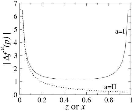
Figure 7: A comparison of the modulus of the typical $\triangle f^{\text{I}}(p)$ and $\triangle f^{\text{II}}(p)$ for some fixed $p$ in an underpopulated momentum region for various values of the lightcone fraction $z$ or $x$. The area covered by the curve of $\triangle f^{\text{I}}(p)$ is clearly more than twice that of $\triangle f^{\text{II}}(p)$.

There are the remaining fourth and fifth terms. For these we have to distinguish the two different incoming gluons raised in point (iii).

• Both flux from overpopulated momentum regions:

  The fourth term of Eq. (88) has $\triangle f^{\text{II}}(xp_{2})=-\triangle f^{\text{I}}(p_{2})>0$ from Eq. (89) (point (v)), as part of the integrand and the fifth has $\triangle f^{\text{I}}(p_{2})$ from Eq. (86). Thus the fourth has a positive contribution to the cross-section and the fifth contributes negatively. Although they both carry the same factor $\triangle f^{\text{I}}(p_{2})$, the fifth term has an extra symmetry factor of one-half and the occupancies of the outgoing particles are smaller than those from the fourth term because the outgoing gluon momenta are in general larger. To see this, the outgoing momenta of the fourth term are $p_{3^{\prime}}+p_{4^{\prime}}=p_{1}+p_{2}-p_{5}$ whereas those of the fifth term are $p_{3}+p_{4}=p_{1}+p_{2}$. $f(p_{3^{\prime}})$ and $f(p_{4^{\prime}})$ will in general be larger than $f(p_{3})$ and $f(p_{4})$ as a consequence. The sum of the fourth and fifth term therefore gives a net positive contribution to $\sigma_{\text{in-medium}}$. Grouping now all the contributions of collinear processes from the final states as well as those in the initial states discussed here, the sum of the four next-to-leading contributions in Eq. (88) are negative so their contribution to the in-medium cross-section is positive.

• One flux from an overpopulated and the other from an underpopulated region:

  In this case the $p_{2}$-centered flux is from an underpopulated region since $p_{1}$ has already been chosen to be from the hard overpopulated region. This is the reverse of situation of 1). From point (iv) the fourth term of Eq. (88) is now negative with $-\triangle f^{\text{I}}(p_{2})<0$ and the fifth becomes positive with $\triangle f^{\text{I}}(p_{2})>0$. The same reasons given in 1) that ensured the sum of the two was positive there now ensure that it is negative. To sum it up, the second and third term of Eq. (88) give a net positive contribution but the fourth and fifth term give a net negative contribution.

  Of course these are not the only contributions because both $C^{>}_{{\cal F}_{1}{\cal F}_{2}}(p_{1})$ and $C^{>}_{{\cal F}_{1}{\cal F}_{2}}(p_{2})$ have an entry in $\sigma_{\text{in-medium}}$ in Eq. (87). In the $C^{>}_{{\cal F}_{1}{\cal F}_{2}}(p_{2})$ entry, the second and third term and also the fourth and fifth term as well would still give net positive contributions because there is not much difference here from case 1). It follows that the collinear processes in the initial states of the two incoming flux in this case tend to have opposing and compensating effects on each other. In general it is hard to tell which contributions will have the upper-hand since it depends to a certain extent both on the value of $p_{1}$ and $p_{2}$, and on how close each of these is to the boundary separating the overpopulated to the under-occupied regions. Thus the collinear processes in the initial states do not have much net effect on the average, however those in the final states are still very much present and positive. One can conclude that there is still enhancing effect on $\sigma_{\text{in-medium}}$ but to a lesser degree than that in 1).

VI In conclusion

Because of the overall positive contributions from the collinear processes together with the fact that these contributions vanish when the interactions occur in the vacuum or when the system is in equilibrium, it means that the in-medium non-equilibrium cross-section is larger or equivalently the out-of-equilibrium interaction rate is higher than what is expected. This is the novel perturbative mechanism for achieving very fast thermalization within 0.6 fm/c at RHIC that we are hoping for. Underlying this mechanism is the non-vanishing of collinear logarithmic terms in a system that is out of equilibrium. We are not aware that this has been pointed out in any existing literature. This is considered in more detail in wip . In closing we have yet to consider here the size of the enhancement which is clearly dependent on how far away from equilibrium the system is, and also we have not considered how the contributions at higher orders will affect our main conclusion, nevertheless a lot of the structures in the various $C(p_{i})$’s, the factors of distributions and the inequalities that they satisfy are shared with those at higher orders. These are better studied and verified numerically than by using the arguments that we have attempted here. All these will be done in the future.

References

- (1) K.H. Ackermann et al., STAR Collaboration, Phys. Rev. Lett. 86, 402 (2001).
- (2) C. Adler et al., STAR Collaboration, Phys. Rev. Lett. 87, 182301 (2001).
- (3) R. Snellings for the STAR Collaboration, Nucl. Phys. A 698, 193c (2002).
- (4) R.A. Lacey for the PHENIX Collaboration, Nucl. Phys. A 698, 559c (2002); K. Adcox et al., PHENIX Collaboration, nucl-ex/0204005.
- (5) I.C. Park for the PHOBOS Collaboration, Nucl. Phys. A 698, 564c (2002).
- (6) J.Y. Ollitrault, Phys. Rev. D 46, 229 (1992).
- (7) P.F. Kolb, J. Sollfrank, and U. Heinz, Phys. Lett. B 459, 667 (1999) and Phys. Rev. C 62, 054909 (2000).
- (8) P.F. Kolb, P. Huovinen, U. Heinz, and H. Heiselberg, Phys. Lett. B 500, 232 (2001); P.F. Kolb, U. Heinz, P. Huovinen, K.J. Eskola, and K. Tuominen, Nucl. Phys. A 696, 197 (2001).
- (9) P. Huovinen, P.F. Kolb, U. Heinz, P.V. Ruuskanen, and S.A. Voloshin, Phys. Lett. B 503, 58 (2001);
- (10) U. Heinz and S.M.H. Wong, Phys. Rev. C 66, 014907 (2002).
- (11) D. Molnár and M. Gyulassy, nucl-th/0102031.
- (12) D. Molnár and M. Gyulassy, nucl-th/0104018.
- (13) D. Molnár and M. Gyulassy, Nucl. Phys. A 697, 495 (2002).
- (14) K. Geiger and B. Müller, Nucl. Phys. B 369, 600 (1992).
- (15) K. Geiger, Phys. Rev. D 46, 4965 and 4986 (1992).
- (16) K. Geiger, Phys. Rep. 258, 237 (1995).
- (17) S.M.H. Wong, Nucl. Phys. A 607, 442 (1996); Phys. Rev. C 54, 2588 (1996); Nucl. Phys. A 638, 527c (1998).
- (18) S.M.H. Wong, Phys. Rev. C 56, 1075 (1997).
- (19) L. McLerran and R. Venugopalan, Phys. Rev. D 49, 2233 and 3352 (1994); Phys. Rev. D 50, 2225 (1994).
- (20) A.H. Mueller, Phys. Lett. B 475, 220 (2000); Nucl. Phys. B 572, 227 (2000).
- (21) R. Baier, A.H. Mueller, D. Schiff, and D.T. Son, Phys. Lett. B 502, 51 (2001).
- (22) E.V. Shuryak and L. Xiong, Phys. Rev. C 49, 2203 (1994).
- (23) T. Kinoshita, J. Math. Phys. 3, 650 (1962).
- (24) T.D. Lee and M. Nauenberg, Phys. Rev. 133, B1549 (1964).
- (25) Work in progress to be reported elsewhere.
- (26) L. Combridge, J. Kripfganz, and J. Ranft, Phys. Lett. B 70, 234 (1977).
- (27) E. Braaten and R.D. Pisarski, Nucl. Phys. B 337, 569 (1990).
- (28) E. Braaten and R.D. Pisarski, Phys. Rev. Lett. 64, 1338 (1990).
- (29) H.A. Weldon, Phys. Rev. D 26, 1394 (1982).
- (30) G. Altarelli and G. Parisi, Nucl. Phys. B 126, 298 (1977).
- (31) V.N. Gribov and L.N. Lipatov, Sov. J. Nucl. Phys. 15, 438 (1972).
- (32) Yu.L. Dokshitzer, JETP 46, 641 (1977).
- (33) R.K. Ellis, W.J. Stirling, and B.R. Webber, QCD and Collider Physics, Cambridge University Press (1996).
- (34) S.M.H. Wong, Phys. Rev. D 64, 025007 (2001).