LMU 04/04

hep-ph/0404220

May 2004

$b$-physics signals of the lightest CP-odd Higgs in the NMSSM at large $\tan\beta$

Gudrun Hiller¹

Ludwig-Maximilians-Universität München, Sektion Physik, Theresienstraße 37
D-80333 München, Germany

We investigate the low energy phenomenology of the lighter pseudoscalar $A_{1}^{0}$ in the NMSSM. The $A_{1}^{0}$ mass can naturally be small due to a global $U(1)_{R}$ symmetry of the Higgs potential, which is only broken by trilinear soft terms. The $A_{1}^{0}$ mass is further protected from renormalization group effects in the large $\tan\beta$ limit. We calculate the $b\to sA_{1}^{0}$ amplitude at leading order in $\tan\beta$ and work out the contributions to rare $K$, $B$ and radiative $\Upsilon$-decays and $B-\bar{B}$ mixing. We obtain constraints on the $A_{1}^{0}$ mass and couplings and show that masses down to ${\cal{O}}(10)$ MeV are allowed. The $b$-physics phenomenology of the NMSSM differs from the MSSM in the appearance of sizeable renormalization effects from neutral Higgses to the photon and gluon dipole operators and the breakdown of the MSSM correlation between the $B_{s}\to\mu^{+}\mu^{-}$ branching ratio and $B_{s}-\bar{B}_{s}$ mixing. For $A_{1}^{0}$ masses above the tau threshold the $A_{1}^{0}$ can be searched for in $b\to s\tau^{+}\tau^{-}$ processes with branching ratios $\stackrel{{\scriptstyle<}}{{{}_{\sim}}}10^{-3}$.

1 Introduction

Sizeable flavor changing neutral current (FCNC) effects in meson decays arise in the minimal supersymmetric Standard Model (MSSM) at large $\tan\beta$, e.g. [1]-[6]. In this model, the amplitude of exchanging neutral Higgses between down-type fermions $f$, i.e. down-type quarks or charged leptons

$$\sum_{S=h^{0},H^{0},A^{0}}\frac{(g_{\bar{f}fS})^{2}}{m_{S}^{2}}\propto-\frac{\cos^{2}(\beta-\alpha)}{m_{h^{0}}^{2}}-\frac{\sin^{2}(\beta-\alpha)}{m_{H^{0}}^{2}}+\frac{1}{m_{A^{0}}^{2}}=0$$ (1)

vanishes. Here, $m_{S}$, $g_{\bar{f}fS}$ denote the Higgs masses and couplings to a fermion pair, respectively and $\alpha$ is the scalar mixing angle. Eq. (1) implies that the Wilson coefficients for $b\to s\ell^{+}\ell^{-}$ decays from scalar and pseudoscalar boson exchange in the MSSM at large $\tan\beta$ are equal with opposite sign [2],[3]. If the relation is broken, interesting effects via operator mixing are induced [7]. In particular, the dipole operators responsible for $b\to s\gamma$ and $b\to sg$ decays receive sizeable contributions from the neutral Higgs bosons. Furthermore, specific contributions to $B-\bar{B}$ mixing from scalar exchange arise. This happens in the presence of more Higgses, such as in the next-to-minimal supersymmetric Standard Model (NMSSM).

The NMSSM is the MSSM extended by a singlet $N$, with the superpotential [8, 9]

$$W=QY_{u}H_{u}U+QY_{d}H_{d}D+LY_{e}H_{d}E+\lambda H_{d}H_{u}N-\frac{1}{3}kN^{3}$$ (2)

The physical NMSSM Higgs sector consists of three scalars $h^{0},H^{0}_{1,2}$ and two pseudoscalars $A_{1,2}^{0}$. As in the minimal model, $\tan\beta=v_{u}/v_{d}$ denotes the ratio of Higgs doublet vevs $v_{u}=<H_{u}^{0}>=v\sin\beta$ and $v_{d}=<H_{d}^{0}>=v\cos\beta$, where $v=\sqrt{2}m_{W}/g\simeq 174$ GeV. The Higgs potential

$$V_{higgs}=V_{soft}+V_{F}+V_{D}$$ (3)

where

$$V_{soft}\! = \!m_{H_{d}}^{2}|H_{d}|^{2}+m_{H_{u}}^{2}|H_{u}|^{2}+m_{N}^{2}|N|^{2}-(\lambda A_{\lambda}H_{d}H_{u}N+h.c.)\!-(\frac{1}{3}kA_{k}N^{3}\!+h.c.)$$ (4)

$$V_{F}\! = \!|\lambda|^{2}\left(|H_{d}|^{2}+|H_{u}|^{2}\right)|N|^{2}+|\lambda H_{d}H_{u}-kN^{2}|^{2}$$ (5)

$$V_{D}\! = \!\frac{g^{2}+g^{\prime 2}}{8}\left(|H_{d}|^{2}-|H_{u}|^{2}\right)+\frac{g^{2}}{2}|H_{u}^{\dagger}H_{d}|^{2}$$ (6)

has a global $U(1)_{R}$ symmetry in the limit of vanishing soft terms $A_{k},A_{\lambda}\to 0$ [10]. If this symmetry is broken only slightly, the model naturally contains a light pseudoscalar. Its mass is given as

$$m_{A_{1}^{0}}^{2}=3kxA_{k}+{\cal{O}}(\frac{1}{\tan\beta})$$ (7)

where $x=<N>$ denotes the vev of the singlet. Note that a small $A_{k}$ remains small under renormalization group running and thus protects $m_{A_{1}^{0}}$.

Lower bounds on CP-odd scalar masses are not very stringent and can be as low as $\sim 100$ MeV [11]. Since the coupling $h^{0}A_{1}^{0}A_{1}^{0}$ is not suppressed the scalar Higgs predominantly decays into the lighter pseudoscalars. This has important consequences for the Tevatron and LHC Higgs searches [10, 12].

The motivation for this work is to find out how and to what extend the NMSSM would signal itself in rare $b$-decays and at the same time, whether existing data provide already bounds on the NMSSM parameter space. We employ the large $\tan\beta\stackrel{{\scriptstyle>}}{{{}_{\sim}}}30$ and small $A_{k}\ll m_{W},x$ limit and no flavor or CP violation other than in the CKM matrix (“minimal flavor violation”). Since a small $A_{\lambda}$ is not stable under radiative corrections, we do not expand in small $A_{\lambda}$ and keep it finite. Our study is based on mostly generic features of the NMSSM. Specific analyses of the NMSSM particle spectrum and parameter space have been carried out in a GUT framework [13] at large $\tan\beta$ [14], with gauge mediated SUSY breaking [15] and with anomaly mediation [16]. For Higgs production in rare $b$-decays in other models, see e.g. [17, 18].

This paper is organized as follows: In Section 2 we calculate the amplitude for $b\to sA_{1}^{0}$ decays at large $\tan\beta$. We discuss the NMSSM parameter space in Section 3. Phenomenological bounds from FCNC decays, $B-\bar{B}$ mixing and $\Upsilon$-decays are worked out in Section 4. In Section 5 we investigate the impact on semileptonic and radiative rare $b$-decays. We also analyse how much the MSSM tree level relation Eq. (1) is broken by loop corrections. We conclude in Section 6. Feynman rules and the NMSSM particle spectrum at large $\tan\beta$ and auxiliary functions are given in Appendix A and B. In Appendix C we give decay rates of the $A_{1}^{0}$ and $b$-decay branching ratios.

2 The $b\to sA_{1}^{0}$ amplitude at large $\tan\beta$

The amplitude for a FCNC $b\to s$ transition into the lightest CP-odd scalar $A_{1}^{0}$ in the NMSSM is induced at one-loop. In the large $\tan\beta$ limit, only two diagrams remain to be calculated, which are shown in Figure 1. (We neglect the strange quark mass). Feynman rules are given in Appendix A.1, see also [19] for the MSSM and [20] for the NMSSM.

The stop chargino wave function correction is identical to the corresponding one in the MSSM. Since the coupling of the $A_{1}^{0}$ to down-type fermions is order $(\tan\beta)^{0}$, the 1PR diagram contributes to the $b\to sA_{1}^{0}$ amplitude at order $\tan\beta$. The vertex correction shown in Figure 1 is the only 1PI diagram linear in $\tan\beta$ because i the $H^{\pm}W^{\mp}A_{1}^{0}$ coupling is $1/\tan\beta$ suppressed since the $A_{1}^{0}$ is predominantly the gauge singlet (the $H^{+}H^{-}A_{1}^{0}$, $W^{+}W^{-}A_{1}^{0}$ vertices are forbidden by CP), ii the coupling of the $A_{1}^{0}$ to up-type quarks is $1/\tan^{2}\beta$, iii the coupling of the $A_{1}^{0}$ to up-type squarks is $1/\tan\beta$ which can be seen from the F-term contribution $|\partial W/\partial H_{u}|^{2}$ and iv the only $\tan\beta$ enhancement comes from the $b_{R}\tilde{t}_{L}\tilde{H}_{d}$ or $b_{R}t_{L}H_{d}$ vertices.

Figure 1: The leading $b\to sA_{1}^{0}$ diagrams at large $\tan\beta$ in the NMSSM.

We obtain the following amplitude

$$i{\cal{A}}(b\to sA_{1}^{0})=-4\frac{G_{F}}{\sqrt{2}}V_{tb}V_{ts}^{*}C_{A}\frac{1}{16\pi^{2}}\bar{s}_{L}b_{R}A_{1}^{0}$$ (8)

where

$$C_{A}=-i\frac{\tan\beta m_{b}}{\sqrt{2}}\left[-\frac{\delta_{-}}{x}\sum_{i=1,2}X_{i}+\lambda m_{t}\sin\theta_{\tilde{t}}\cos\theta_{\tilde{t}}\sum_{l,j=1,2}Y_{lj}\right]$$ (9)

and $\delta_{-}$ parametrizes the $A_{1}^{0}\bar{b}b$ coupling, see Eq. (A-10). The $X,Y$ terms in Eq. (9) result from the wave function and vertex correction, respectively . They are written as

$$X_{i} = m_{\chi_{i}}U_{i2}\left[\sqrt{2}m_{W}V_{i1}\left(-D_{3}(y_{c,i})+D_{3}(y_{1,i})\cos^{2}\theta_{\tilde{t}}+D_{3}(y_{2,i})\sin^{2}\theta_{\tilde{t}}\right)\right.$$ (10)

$$- \left.m_{t}V_{i2}\sin\theta_{\tilde{t}}\cos\theta_{\tilde{t}}\left(D_{3}(y_{1i})-D_{3}(y_{2i})\right)\right]$$

$$Y_{lj} = V_{j2}U_{l2}\left[\left(y_{1j}U_{j2}V_{l2}-\frac{m_{\chi_{l}}}{m_{\chi_{j}}}U_{l2}V_{j2}\right)D_{2}(y_{1j},z_{lj})\right.$$ (11)

$$\left.\hskip 28.45274pt-\left(y_{2j}U_{j2}V_{l2}-\frac{m_{\chi_{l}}}{m_{\chi_{j}}}U_{l2}V_{j2}\right)D_{2}(y_{2j},z_{lj})\right]$$

where

$$y_{kj}=\frac{m_{\tilde{t}_{k}}^{2}}{m_{\chi_{j}}^{2}}\,,~{}~{}~{}~{}~{}~{}y_{cj}=\frac{m_{\tilde{c}}^{2}}{m_{\chi_{j}}^{2}}\,,~{}~{}~{}~{}~{}~{}z_{lj}=\frac{m_{\chi_{l}}^{2}}{m_{\chi_{j}}^{2}}$$ (12)

and $m_{\tilde{t}_{k}},m_{\tilde{c}},m_{\chi_{l}}$ denote the stop, scharm and chargino masses. The stop mixing angle $\theta_{\tilde{t}}$, the chargino mixing matrices $U,V$ and the loop functions $D_{2},D_{3}$ are defined in Appendix B. We used unitarity of the CKM matrix and neglected squark mixing other than for stops and mass splitting between the first two generations. The $b\to dA_{1}^{0}$ amplitude is obtained by replacing ‘$s$’ by ‘$d$’ everywhere in Eq. (8). The $s\to dA_{1}^{0}$ amplitude is given correspondingly with also changing $m_{b}$ to $m_{s}$ in Eq. (9). Note that our calculation holds for $|\delta_{\pm}v/x|<\tan\beta$, see Appendix A. E.g. for larger values of $\delta_{-}v/x$ the $A_{1}^{0}$ looses its mostly-singlet nature and more $b\to sA_{1}^{0}$ diagrams need to be calculated.

The coupling $C_{A}$ vanishes if the super GIM mechanism is active, that is either all squark masses are degenerate or $m_{\tilde{c}}=m_{\tilde{t}_{1}}$ and $\theta_{\tilde{t}}=0$ (or $\pi$) or $m_{\tilde{c}}=m_{\tilde{t}_{2}}$ and $\theta_{\tilde{t}}=\pi/2$. We estimate the generic size of $C_{A}$ with order one stop mixing as

$$|C_{A}|\simeq{\cal{O}}(\delta_{-}\tan\beta m_{b}m_{t}\frac{m_{\chi}}{x})+{\cal{O}}(\lambda\tan\beta m_{b}m_{t})$$ (13)

Since $\lambda x$ is the NMSSM $\mu$-term which sets the mass scale for the charginos, both terms are of comparable size.

3 Viable points in the NMSSM parameter space

The relevant NMSSM parameter space consists of $\lambda,k$ from the superpotential, the soft breaking terms $A_{\lambda},A_{k}$, the gaugino mass $m_{2}$, stop and scharm masses, the stop mixing angle $\theta_{\tilde{t}}$ and $\tan\beta$. We evaluate all parameters at the electroweak scale.

The dimensionless couplings $\lambda$ and $k$ run towards smaller values, e.g. $\lambda^{2}+k^{2}\stackrel{{\scriptstyle<}}{{{}_{\sim}}}0.6$ at the electroweak scale for $\lambda,k\stackrel{{\scriptstyle<}}{{{}_{\sim}}}2\pi$ at the high, GUT scale [21]. We use $|\lambda|,|k|\leq 1$. Similar to the MSSM, electroweak symmetry breaking at large $\tan\beta$ requires [14]

$$m_{H_{u}}^{2}=-(\lambda x)^{2}-\frac{m_{Z}^{2}}{2}$$ (14)

and therefore the product of $\lambda$ and $x$ should not exceed $\sim{\cal{O}}(1)$ TeV to avoid fine tuning. On the other hand, the chargino mass scale is driven by $\lambda x$, which should be at least ${\cal{O}}(100)$ GeV by experimental search limits. We assume the singlet vev $x$ to be of the order of the Fermi scale $v$, or at least not smaller than 100 GeV and not bigger than 3 TeV. If $x$ exceeds this value, its relation to the other vevs becomes unnatural and the model does not give a solution to the $\mu$ problem [8]. Hence, the size of $\lambda$ is bounded from below as $|\lambda|\stackrel{{\scriptstyle>}}{{{}_{\sim}}}\mbox{few}\cdot 10^{-2}$ [15, 21]. Further, the extremization condition

$$m_{H_{d}}^{2}=-\lambda^{2}(x^{2}+v^{2})+m_{A}^{2}+\frac{m_{Z}^{2}}{2}$$ (15)

where we defined

$$m_{A}^{2}\equiv\lambda(A_{\lambda}+kx)x\tan\beta$$ (16)

implies some cancellation among the $\tan\beta$ enhanced terms as [14]

$$A_{\lambda}+kx\sim\frac{{\cal{O}}(100-1000\,\mbox{GeV})}{\tan\beta}$$ (17)

Note that $m_{A}$ sets the scale for the heavy Higgses $A_{2}^{0},H_{2}^{0}$ and $H^{\pm}$, see Appendix A.

The NMSSM is further constrained by non-observation of Higgses and superpartners. At large $\tan\beta$, the mass of the lightest scalar at tree level is given as

$$m_{h^{0}}^{2}\simeq m_{Z}^{2}-\frac{\lambda^{4}v^{2}}{k^{2}}$$ (18)

where we expanded Eq. (A-22) in $m_{Z}^{2}/4k^{2}x^{2}\ll 1$ and $\lambda^{2}v/k^{2}x\ll 1$. In this approximation also $m_{H_{1}^{0}}^{2}\simeq 4k^{2}x^{2}+\frac{\lambda^{4}v^{2}}{k^{2}}$ and the scalar mixing angle $\theta$ is small. Like in the MSSM, the $h^{0}$ tree level mass cannot be bigger than the $Z$-mass because the raising of its upper bound in the NMSSM is suppressed by large $\tan\beta$. To be phenomenologically viable, $m_{h^{0}}$ has to be lifted by radiative corrections above the current search limit as in the MSSM [22]. We require the scalar tree level mass to be bigger than 89 GeV, which favors small $\lambda$ or $\lambda/k$ less than one. We allow for $|m_{2}|\leq 1$ TeV and check that the charginos are heavier than 90 GeV. We treat the pseudoscalar masses $m_{A_{1}^{0}}$ and $m_{A_{2}^{0}}$ with $m_{A_{2}^{0}}\stackrel{{\scriptstyle>}}{{{}_{\sim}}}130$ GeV as free parameters, i.e. adjust $A_{k}$ and $A_{\lambda}$ accordingly. The squark masses and stop mixing angle are effective parameters with $m_{\tilde{t}_{1}}>90$ GeV and $m_{\tilde{t}_{2}},m_{\tilde{c}}\sim 1$ TeV and we do not relate them to fundamental parameters in the Lagrangian.

The down-type fermion-$A_{1}^{0}$ vertex is proportional to $\delta_{-}v/x$, see Eq. (A-24). From Eqs. (16) and (17) we obtain

$$\frac{v}{x}\delta_{-} = \frac{v}{x}\left[-3\frac{k\lambda x^{2}}{m_{A}^{2}}\tan\beta+1\right]\simeq\pm 3\frac{kvm_{\chi}}{m_{A}^{2}}\tan\beta$$ (19)

where the second equation is a good approximation for not too large $m_{A}\stackrel{{\scriptstyle<}}{{{}_{\sim}}}500$ GeV. It then gives a lower bound on $|\delta_{-}v/x|$. In particular, for $\tan\beta=30$, $m_{A}\stackrel{{\scriptstyle<}}{{{}_{\sim}}}500\,(200)\,(130)$ GeV and the ranges of parameters given in the preceding paragraphs, we obtain $|\delta_{-}v/x|\stackrel{{\scriptstyle>}}{{{}_{\sim}}}0.1\,(1)\,(3)$. For larger values of $m_{A}$ cancellations between the two terms in Eq. (19) are possible. Note that the $\tan\beta$ factor is only a formal enhancement, since it is cancelled by the one in $m_{A}^{2}$. We find that $|\delta_{-}v/x|\leq 62\,(16)$ for $m_{A}\geq 500\,(1000)$ GeV. Note that the small $A_{\lambda}\ll kx$ limit with $\delta_{-}\simeq-2$ makes its hard to satisfy Eq.(17).

4 Phenomenology of the light ${A_{1}^{0}}$

We work out constraints on the mass of the $A_{1}^{0}$ in the NMSSM at large $\tan\beta$ from $A_{1}^{0}$ production in rare decays (Section 4.1), $\bar{B}-B$ mixing (Section 4.2) and $B_{s}\to\mu^{+}\mu^{-}$ decays (Section 4.3). We make use of the $b\to sA_{1}^{0}$ amplitude calculated in Section 2. We scan the parameter space in the regions discussed in Section 3. All FCNC bounds can be evaded by a sufficiently tuned-in super GIM mechanism, see Section 2. To quantify this, we demand in our numerical analysis for the mass splitting $m_{\tilde{t}_{2}}-m_{\tilde{t}_{1}}>50$ GeV while varying $m_{\tilde{t}_{1}}$ and for the stop mixing $\epsilon<\theta_{\tilde{t}}<\pi/2-\epsilon$ or $\pi/2+\epsilon<\theta_{\tilde{t}}<\pi-\epsilon$ with $\epsilon=0.05$. Bounds from other processes are discussed in Section 4.4.

Many experimental constraints we use here apply only if the $A_{1}^{0}$ is sufficiently stable, i.e. leaves the detector as missing energy. This happens if the pseudoscalar width is smaller than $E_{A}/(m_{A_{1}^{0}}\,d)$, where $d\sim{\cal{O}}(10)$ m is the size of the detector and $E_{A}$ the $A_{1}^{0}$ energy in the lab frame. We work out bounds on $m_{A_{1}^{0}}$ as a function of $|\delta_{-}v/x|$. If this coupling gets smaller, the pseudoscalar decay rate decreases, and a heavier Higgs will become missing energy and vice versa. For decay rates of the $A_{1}^{0}$, see Appendix C.

For Higgs masses below $2m_{\mu}$ only the $e^{+}e^{-}$ and $\gamma\gamma$ decay channels are relevant. (The $A_{1}^{0}\to\pi^{0}\gamma$ decay is forbidden by CP and angular momentum conservation and the $A_{1}^{0}\to\pi^{0}\gamma\gamma$ decay is suppressed with respect to the dielectron mode by phase space and powers of $\alpha$). The $\gamma\gamma$ mode can compete with $A_{1}^{0}\to f\bar{f}$ decays only near the dimuon threshold. This weakens the missing energy bounds in that region.

The point we want to make is to show that in the NMSSM ${A_{1}^{0}}$ masses in the GeV range and below are not ruled out. This is summarized in Figure 2. For details see the following subsections. All experminental bounds are taken at 90 % confidence level. The requisite $b\to A_{1}^{0}$ branching ratios are given in Appendix C. We recall that our approximation breaks down if $|\delta_{\pm}v/x|$ approaches $\tan\beta$.

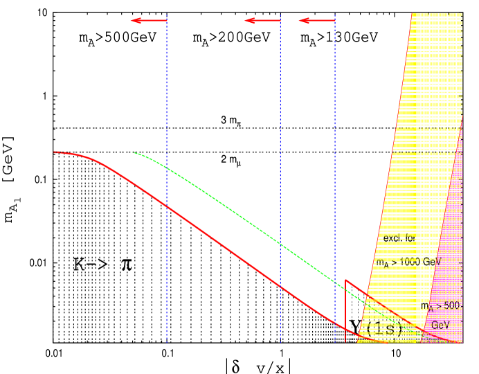
Figure 2: Constraints on the $A_{1}^{0}$ mass as a function of $|\delta_{-}v/x|$ at $\tan\beta=30$ in the NMSSM. Shaded regions are excluded. The left bottom corner is excluded by rare $K$-decay, see Eq. (21). The triangular region to the lower right is obtained from radiative $\Upsilon(1s)$ decays, see Eq. (35). The region to the left of the vertical dashed blue lines can only be reached if $m_{A}$ is bigger than the value indicated, see Section 3. Constraints from $\Delta m_{d}$ are given for $m_{A}\geq 500$ GeV and $m_{A}\geq 1000$ GeV. We also show the missing energy condition for $B\to K$ decays given in Eq. (20) (dashed green line). The vertical dashed lines indicate $m_{A_{1}^{0}}=2m_{\mu}$ and $3m_{\pi}$.

4.1 Rare $K$ and $B$-decays

If the Higgs boson is light enough, it can be produced in $b\to sA_{1}^{0}$ or $s\to dA_{1}^{0}$ processes. We analyze what bounds exist depending on the mass of the $A_{1}^{0}$.

4.1.1 $2m_{e}<m_{A_{1}^{0}}<2m_{\mu}$

When produced in rare $B$-meson decays the $A_{1}^{0}$ decays outside of the detector if

$$m_{A_{1}^{0}}\stackrel{{\scriptstyle<}}{{{}_{\sim}}}17\;\mbox{MeV}/|\delta_{-}v/x|$$ (20)

In this region the CLEO bound ${\cal{B}}(B\to K_{S}^{0}X^{0})<5.3\cdot 10^{-5}$ [23] applies. There is a similar missing energy bound from BaBar ${\cal{B}}(B^{-}\to K^{-}\nu\bar{\nu})<7.0\cdot 10^{-5}$ [24] . We find that masses in the range given in Eq. (20) are disfavored since the $B\to KA_{1}^{0}$ decay, see Eq. (C-8), would happen too rapidly for most of the parameter space, although cannot rigorously be excluded. We stress that the size of the coupling $C_{A}$ can be quite large, see Eq. (13) and already ${\cal{B}}(B\to X_{s}A_{1}^{0})<1$ cuts out a fraction of NMSSM points.

Rare decays into $e^{+}e^{-}$ constrain Higgs masses below the muon threshold. However, the measurements of the inclusive $B\to X_{s}e^{+}e^{-}$ branching ratios contain cuts on the dilepton mass $m_{ee}\stackrel{{\scriptstyle>}}{{{}_{\sim}}}2m_{\mu}$ [25, 26]. In the analysis of $B\to K^{(*)}e^{+}e^{-}$ decays Belle applies $m_{ee}>0.14$ GeV [27], whereas BaBar [28] has no cut, but the efficiency is low in that region due to conversion photons. Likewise, measurements of $K^{+}\to\pi^{+}e^{+}e^{-}$ decays employ a high mass trigger [29]. Since also close to $2m_{\mu}$ the two-photon decay of the $A_{1}^{0}$ becomes sizeable, we do not take the $e^{+}e^{-}$ data into account.

The bound ${\cal{B}}(K^{+}\to\pi^{+}A_{1}^{0})<4.5\cdot 10^{-11}$ [30] is applicable if the $A_{1}^{0}$ becomes sufficiently stable to escape the detector. This happens for masses

$$m_{A_{1}^{0}}\stackrel{{\scriptstyle<}}{{{}_{\sim}}}5\,\mbox{MeV}/|\delta_{-}v/x|$$ (21)

which then are excluded. The $K$-decay bound is five orders of magnitude better than the one from $B\to K$ decays, because the CKM and mass suppression of the $K\to\pi A_{1}^{0}$ decay rate is compensated by the difference in life time $|V_{td}/V_{ts}|^{2}(m_{K}/m_{B})^{3}\tau(K^{+})/\tau(B^{+})\simeq 0.24$ [31], see Eq. (C-8) and its $K\to\pi$ counterpart.

4.1.2 $2m_{\mu}<m_{A_{1}^{0}}<2m_{\tau}$

$A_{1}^{0}$ decays into a muon pair are included in $B\to X_{s}\mu^{+}\mu^{-}$ signals. Comparison of the $B\to X_{s}A_{1}^{0}$ branching ratio, see Eq. (C-7), with the data ${\cal{B}}(B\to X_{s}\mu^{+}\mu^{-})\leq 10.4\cdot 10^{-6}$ [7, 25, 26] shows that this is very unlikely. The same happens in $K\to\pi\mu^{+}\mu^{-}$ decays, which for $m_{A_{1}^{0}}<m_{K}-m_{\pi}$ can hide a pseudoscalar decaying into muons. With ${\cal{B}}(K^{+}\to\pi^{+}\mu^{+}\mu^{-})\leq 10.4\cdot 10^{-8}$ [31] only a tiny number of points survives the scan. All allowed points are at the GIM boundary $\theta_{\tilde{t}}\simeq\pi/2$, which is set by our value of the cut-off $\epsilon$.

Above the $3\pi$ threshold sizeable hadronic decays open up. (The $A_{1}^{0}\to 2\pi\gamma$ decay is suppressed with respect to the dimuon channel by phase space and $\alpha$, whereas $A_{1}^{0}\to 2\pi$ decay is forbidden by CP invariance.) For the $A_{1}^{0}$ decaying hadronically into a strange final state we use ${\cal{B}}(b\to sg)<9\%$ [32]. This thins out the NMSSM model space for $3m_{\pi}<m_{A_{1}^{0}}<2m_{\tau}$, but cannot exclude this region. (We use ${\cal{B}}(b\to sA_{1}^{0})>{\cal{B}}(b\to dA_{1}^{0})$.)

4.1.3 $2m_{\tau}<m_{A_{1}^{0}}\stackrel{{\scriptstyle<}}{{{}_{\sim}}}m_{B}$

If the $A_{1}^{0}$ is above the tau threshold, most of the time it decays into $\tau^{+}\tau^{-}$ because its coupling to $c\bar{c}$ is $\tan^{2}\beta$ suppressed. Similar to the constraint on the hadronically decaying pseudoscalar, see Section 4.1.2, the mildly model-dependent bound ${\cal{B}}(B\to X_{s}\tau^{+}\tau^{-})<5$ % [33] is not a challenge to the light CP-odd Higgs scenario.

4.2 NMSSM neutral Higgs contributions to $B-\bar{B}$ mixing

We calculate the contribution to $B-\bar{B}$ mixing from pseudoscalar $A_{1,2}^{0}$ and scalar $h^{0},H_{1,2}^{0}$ Higgs exchange in the NMSSM at large $\tan\beta$. It arises at two-loop from double insertion of the FCNC $\bar{s}b$-Higgs vertices such as generated by the diagrams in Figure 1 for the $A_{1}^{0}$ and an intermediate boson propagator. The dominant diagrams induced by the heavy Higgses, i.e. the ones other than the lightest CP-odd scalar are the wave function corrections contributions with $A_{2}^{0},H_{2}^{0}$ exchange, see the Feynman rules in Appendix A.1. They can compete with one-loop contributions such as the Standard Model (SM) box diagrams due to their $\tan^{4}\beta$ enhancement. Contributions from $h^{0},H_{1}^{0}$ are subleading in $\tan\beta$. We use an effective Hamiltonian ($q=d,s$)

$${\cal{H}}_{eff}^{\Delta B=2}=\frac{G_{F}^{2}m_{W}^{2}}{16\pi^{2}}(V_{tb}{V_{tq}^{*}})^{2}\sum_{i}C_{i}Q_{i}$$ (22)

where some of the relevant operators are written as, see e.g. [6]

$$Q^{VLL} = (\bar{q}_{L}\gamma_{\mu}b_{L})(\bar{q}_{L}\gamma^{\mu}b_{L})$$ (23)

$$Q_{1}^{SRR} = (\bar{q}_{L}b_{R})(\bar{q}_{L}b_{R})$$ (24)

$$Q_{1}^{SLR} = (\bar{q}_{R}b_{L})(\bar{q}_{L}b_{R})$$ (25)

The SM contribution is in the coefficient $C^{VLL}$. The $A_{2}^{0},H_{2}^{0}$ masses are degenerate at large $\tan\beta$ and their respective contributions to $Q_{1}^{SRR}$ cancel each other just like in the MSSM, see Eq. (1). They do, however, contribute to the operator $Q_{1}^{SLR}$ at order $m_{q}/m_{b}$, and are important for $B_{s}$-mesons. (This is the famous double penguin (DP) contribution of the MSSM [5, 6].)

We obtain at order $\tan^{2}\beta/m_{A_{1}^{0}}^{2}$ in the NMSSM from $A_{1}^{0}$ boson exchange

$$C_{1}^{SRR}(\mu_{t})=-\frac{1}{4\pi^{2}}\frac{C_{A}^{2}}{m_{W}^{2}m_{A_{1}^{0}}^{2}}$$ (26)

at the high, electroweak (matching) scale $\mu_{t}$. Finite widths effects are neglected. We define the size of the $B_{q}-\bar{B}_{q}$ mass difference $\Delta m_{q}$ with respect to its SM value as

$$\frac{\Delta m_{q}}{(\Delta m_{q})_{SM}}=1+f_{q}$$ (27)

where

$$f_{q}=\frac{\bar{P}_{1}^{SLL}}{S_{0}(\mu_{t})}C_{1}^{SRR}(\mu_{t})$$ (28)

and $S_{0}(\mu_{t})=2.38$ and $\bar{P}_{1}^{SLL}=-0.37$ [6]. In Eq. (28) the NMSSM contribution to $\Delta m_{d}$ by neutral Higgs exchange in the $m_{q}=0$ limit has been given. To be in agreement with data we require $f_{d}>-0.6$ ($f_{d}$ is negative). This includes $20$ % uncertainty and allows for cancellations between the $A_{1}^{0}$ contribution and the charged Higgs, chargino boxes and the double penguins. We assume similar sizes as in the MSSM, where $-0.2\stackrel{{\scriptstyle<}}{{{}_{\sim}}}f_{d}^{H^{\pm}}+f_{d}^{\chi^{\pm}}+f_{d}^{DP}\stackrel{{\scriptstyle<}}{{{}_{\sim}}}0.4$ [6]. We find constraints for larger values of $|\delta_{-}v/x|$ and $m_{A}\geq 500$ GeV, which are displayed in Figure 2 for $\tan\beta=30$. The other branch with $1+f_{d}<0$, where the NMSSM correction is larger than the SM box gives very similar constraints and is not shown. The leading $A_{1}^{0}$ contribution to $B-\bar{B}$ mixing is universal in minimal flavor violation, $f_{d}=f_{s}$, since we neglect light quark masses.

4.3 $B_{s}\to\mu^{+}\mu^{-}$ decays

We work out the contributions to $B_{s}\to\mu^{+}\mu^{-}$ decays from neutral Higgs exchanges in the large $\tan\beta$ limit of the NMSSM. With the effective Hamiltonian

$${\cal{H}}_{eff}=-\frac{G_{F}}{\sqrt{2}}V_{tb}V_{ts}^{*}\sum_{i}C_{i}{\cal{O}}_{i}$$ (29)

where

$${\cal{O}}_{S}=\frac{e^{2}}{16\pi^{2}}\bar{s}_{L}b_{R}\bar{\ell}\ell\,,~{}~{}~{}~{}~{}~{}{\cal{O}}_{P}=\frac{e^{2}}{16\pi^{2}}\bar{s}_{L}b_{R}\bar{\ell}\gamma_{5}\ell$$ (30)

we obtain at the electroweak scale (in parentheses is given the particle that induces a particular Wilson coefficient)

$$C_{S}=C_{S}(H_{2}^{0})=-C_{P}(A_{2}^{0})\,,~{}~{}~{}~{}~{}~{}C_{P}=C_{P}(A_{1}^{0})+C_{P}(A_{2}^{0})$$ (31)

where

$$C_{P}(A_{1}^{0}) = m_{b}m_{\ell}\tan\beta\frac{v}{4m_{W}^{2}\sin^{2}\theta_{W}}\left(\frac{v\delta_{-}}{x}\right)\frac{1}{m_{B_{s}}^{2}-m_{A_{1}^{0}}^{2}}$$ (32)

$$\times \left[-\frac{\delta_{-}}{x}\sum_{i=1,2}X_{i}+\lambda m_{t}\sin\theta_{\tilde{t}}\cos\theta_{\tilde{t}}\sum_{l,j=1,2}Y_{lj}\right]$$

$$C_{P}(A_{2}^{0}) = m_{b}m_{\ell}\tan^{3}\beta\frac{1}{4m_{A}^{2}m_{W}^{2}\sin^{2}\theta_{W}}\sum_{i=1,2}X_{i}$$ (33)

The expressions for $X$ and $Y$ are given in Section 2. Our result for the $A^{0}_{2},H^{0}_{2}$ contributions agrees with the corresponding MSSM calculations [3]. Note that the contributions from $A^{0}_{2}$ and $H^{0}_{2}$ are equal with opposite sign. Similar to $B-\bar{B}$ mixing discussed in Section 4.2, the scalars $h^{0}$ and $H_{1}^{0}$ contribute at subleading order in $\tan\beta$.

The coefficients $C_{S,P}$ are model-independently constrained by data on the $B_{s}\to\mu^{+}\mu^{-}$ branching ratio. With ${\cal{B}}(B_{s}\to\mu^{+}\mu^{-})<5.8\cdot 10^{-7}$ [34] we obtain at the scale $\mu=m_{W}$

$$\sqrt{|C_{S}|^{2}+|C_{P}+\delta_{10}|^{2}}\leq 1.3\Bigg{[}\frac{{\mathcal{B}}(B_{s}\to\mu^{+}\mu^{-})}{5.8\times 10^{-7}}\Bigg{]}^{1/2}\Bigg{[}\frac{238\,\mbox{MeV}}{f_{B_{s}}}\Bigg{]}$$ (34)

Here, $\delta_{10}$ stems from the operator ${\cal{O}}_{10}\propto\bar{s}_{L}\gamma_{\mu}b_{L}\bar{\ell}\gamma^{\mu}\gamma_{5}\ell$, see [7] for details. We find with $\delta_{10}^{SM}=-0.095$ at $\tan\beta=30$ the upper limits $|\delta_{-}v/x|\stackrel{{\scriptstyle<}}{{{}_{\sim}}}42\,(16)$ for $m_{A}=500\,(1000)$ GeV, which are are weaker than the corresponding $\Delta m_{d}$ ones. The expressions for the CKM suppressed $B_{d}\to\mu^{+}\mu^{-}$ decay are readily obtained. Its experimental constraint is not as good as the $B_{s}$ one, but we can cut out both $m_{A_{1}^{0}}\simeq m_{B_{d}}$ and $m_{A_{1}^{0}}\simeq m_{B_{s}}$.

4.4 Non-FCNC bounds

The bounds from radiative $\Upsilon$-decays apply if the $A_{1}^{0}$ leaves the detector unseen [31, 36]. Due to the larger boost the critical width to do so is larger than in $B$-meson decays by $m_{\Upsilon}/m_{B}$. We use ${\cal{B}}(\Upsilon(1s)\to A^{0}\gamma)<1.3\cdot 10^{-5}$ [36] and obtain with Eq. (C-10)

$$|\delta_{-}v/x|\stackrel{{\scriptstyle<}}{{{}_{\sim}}}3.7~{}~{}~{}~{}~{}\mbox{ for}~{}~{}~{}m_{A_{1}^{0}}\stackrel{{\scriptstyle<}}{{{}_{\sim}}}23\,\mbox{MeV}/|\delta_{-}v/x|<2m_{\mu}$$ (35)

Furthermore, we get an upper bound $|\delta_{-}v/x|\stackrel{{\scriptstyle<}}{{{}_{\sim}}}100$ from ${\cal{B}}(\Upsilon(1s)\to A_{1}^{0}\gamma)<1$.

Mass bounds from hadronic collisions are not better than few to 200 MeV and astro physics gives $m_{A_{1}^{0}}\stackrel{{\scriptstyle>}}{{{}_{\sim}}}0.2$ MeV [31], which contain some model dependence.

5 Implications for $b\to s\ell^{+}\ell^{-}$ and $b\to s\gamma,g$

Similar to the operators ${\mathcal{O}}_{S,P}$ discussed in Section 4.3, the NMSSM Higgs sector also induces contributions to 4-Fermi operators with quarks and leptons ($f$ denotes a fermion)

$${\cal{O}}_{L}^{f}=\bar{s}_{L}b_{R}\bar{f}_{R}f_{L}\,,\quad{\cal{O}}_{R}^{f}=\bar{s}_{L}b_{R}\bar{f}_{L}f_{R}$$ (36)

where

$$C_{L,R}^{f}=\frac{e^{2}}{16\pi^{2}}\frac{m_{f}}{m_{\mu}}(C_{S}\mp C_{P})$$ (37)

These couplings arise in the NMSSM at large $\tan\beta$, where

$$C_{S}-C_{P}=-2C_{P}(A_{2}^{0})-C_{P}(A_{1}^{0})\,,~{}~{}~{}~{}~{}~{}C_{S}+C_{P}=C_{P}(A_{1}^{0})$$ (38)

This is different from the MSSM, where the $A_{1}^{0}$ contribution is absent and the sum of $C_{S}$ and $C_{P}$ and hence $C_{R}^{f}$ vanish. We discuss corrections to this tree level statement in Section 5.1. All Wilson coefficients refer to the Hamiltonian in Eq. (29) and are evaluated at the scale $\mu=m_{W}$ unless otherwise stated.

The constraint given in Eq. (34) implies for the Wilson coefficients for $b$-quarks (we update the findings of Ref. [7] with the improved $B_{s}\to\mu^{+}\mu^{-}$ bound [34])

$$\sqrt{|C_{L}^{b}|^{2}+|C_{R}^{b}|^{2}}\stackrel{{\scriptstyle<}}{{{}_{\sim}}}0.03$$ (39)

The operators ${\mathcal{O}}_{L,R}^{b}$ enter radiative and semileptonic rare $b\to s$ decays at one-loop [7, 37]. With the bound in Eq. (39) the new physics effect from ${\mathcal{O}}_{L}^{b}$ is small, at the percent level [7]. However, the renormalization effect induced at leading log by ${\cal{O}}_{R}^{b}$ can be large for the photon and gluon dipole operators ${\cal{O}}_{7}$ and ${\cal{O}}_{8}$, which can be written as

$${\cal{O}}_{7}=\frac{e}{16\pi^{2}}m_{b}\bar{s}_{L}\sigma_{\mu\nu}b_{R}F^{\mu\nu},\quad{\cal{O}}_{8}=\frac{g_{s}}{16\pi^{2}}m_{b}\bar{s}_{L\alpha}\sigma_{\mu\nu}T^{a}_{\alpha\beta}b_{R\beta}G^{a\mu\nu}$$ (40)

To be specific, we normalize their coefficients to the ones in the SM, and denote this ratio by $\xi$, such that $\xi^{SM}=1$. With (see [7] for details)

$$\xi_{7}(m_{b}) = 0.514+0.450\,\xi_{7}(m_{W})+0.035\,\xi_{8}(m_{W})-2.319\,C_{R}^{b}\,,$$ (41)

$$\xi_{8}(m_{b}) = 0.542+0.458\,\xi_{8}(m_{W})+19.790\,C_{R}^{b}$$ (42)

and Eq. (39) corrections of up to $7\%$ and $59\%$ to $\xi_{7}$ and $\xi_{8}$ are possible. This has impact on the extraction of Wilson coefficients in $b\to s\gamma$, $b\to sg$ and $b\to s\ell^{+}\ell^{-}$ decays [7]. For a full analysis of these decays, also the matching contributions to $C_{7,8}$ from neutral Higgs loops in the large $\tan\beta$ NMSSM have to be calculated. Note that $\tan\beta$ enhanced corrections to the $b$-quark mass, CKM elements and FCNCs from non-holomorphic terms arise [1, 5, 6]. We leave this for future work.

5.1 Estimates of $C_{S}+C_{P}$ and $C_{R}^{b}$

We work out the NMSSM reach in $C_{S}+C_{P}$ by taking into account all constraints discussed in the previous Sections 3 and 4. The value of $C_{S}+C_{P}$ can saturate its upper bound given in Eq. (34) for large ranges of the parameter space. If the $A_{1}^{0}$ gets very light, however, the $b\to sA_{1}^{0}$ coupling $C_{A}$ has to decrease and $C_{S}+C_{P}$ is small, e.g. for $m_{A_{1}^{0}}=10$ MeV is $|C_{S}+C_{P}|\leq 0.06$. For intermediate masses the $A_{1}^{0}$ contribution dominates over the one from the heavy pseudoscalar, that is $|C_{P}|\gg C_{S}$ and $|C_{R}^{b}|\simeq|C_{L}^{b}|\stackrel{{\scriptstyle<}}{{{}_{\sim}}}0.024$. This is illustrated in Figure 3, where we show $C_{S}+C_{P}$ as a function of $\sqrt{|C_{S}|^{2}+|C_{P}+\delta_{10}^{SM}|^{2}}\propto\sqrt{{\cal{B}}(B_{s}\to\mu^{+}\mu^{-})}$ , see Eq. (34), for $m_{A}=500$ GeV and different values of $m_{A_{1}^{0}}$.

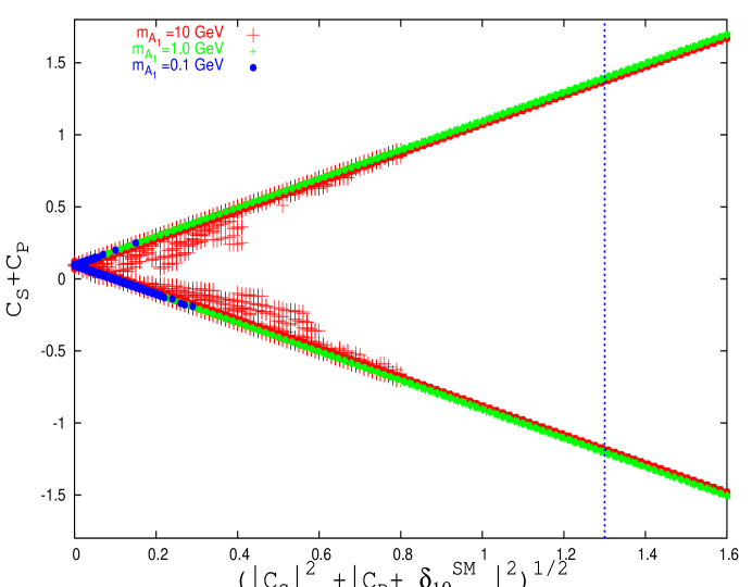
Figure 3: The correlation between $C_{S}+C_{P}$ and $\sqrt{|C_{S}|^{2}+|C_{P}+\delta_{10}^{SM}|^{2}}$ in the NMSSM for $\tan\beta=30$, $m_{A}=500$ GeV and $m_{A_{1}^{0}}=0.1,1$ and $10$ GeV. Also shown is the experimental upper bound given in Eq. (34) (dashed line).

In the MSSM the size of $C_{S}+C_{P}$ is driven by the relation Eq. (1), which is not protected from radiative corrections. To study their size we employ the two-loop calculation encoded in FeynHiggs v. 2.02 [38]. By scanning the MSSM parameter space we find

$$|\frac{C_{S}+C_{P}}{C_{S}-C_{P}}|_{\mbox{\scriptsize\it MSSM}}<0.2~{}~{}~{}~{}\mbox{or}~{}~{}~{}~{}|C_{S}+C_{P}|_{\mbox{\scriptsize\it MSSM}}<0.08~{}~{}~{}~{}\mbox{and}~{}~{}~{}~{}|C_{R}^{b}|_{\mbox{\scriptsize\it MSSM}}<1.3\cdot 10^{-3}$$ (43)

The smallness of $C_{S}+C_{P}$ is a feature of the Higgs sector of the MSSM. It holds also with flavor violation beyond the CKM matrix. As a result, the logarithmic renormalization of the dipole operators from neutral (pseudo)scalars is tiny in this model. For example, consider additional right handed currents, which induce contributions to the helicity flipped operators ${\cal{O}}^{\prime}_{i}$, i.e. the ones obtained from ${\cal{O}}_{i}$ with right $R$ and left $L$ chiralities interchanged. In this case, $C_{S}^{\prime}-C_{P}^{\prime}$ mixes onto the flipped dipole operators ${\cal{O}}^{\prime}_{7,8}$, but $C_{S}^{\prime}=C_{P}^{\prime}$ in the large $\tan\beta$ MSSM [5].

6 Conclusions

We investigated the phenomenology of the light pseudoscalar $A_{1}^{0}$ which lives in the NMSSM spectrum at large $\tan\beta$. The $A_{1}^{0}$ has suppressed gauge interactions but couples to Higgses and down-type matter. We calculated the $b\to sA_{1}^{0}$ amplitude at leading order in $\tan\beta$. Based on this, we estimated the NMSSM contributions to rare $K$, $B$ and radiative $\Upsilon$-decays with the $A_{1}^{0}$ in the final state, $B_{s}\to\mu^{+}\mu^{-}$ decays and $B-\bar{B}$ mixing. We showed that low energy data provide constraints on the $A_{1}^{0}$ mass and couplings, but leave masses down to ${\cal{O}}(10)$ MeV viable, see Figure 2. The $A_{1}^{0}$ predominantly decays into $\tau^{+}\tau^{-}$ for $2m_{\tau}<m_{A_{1}^{0}}<2m_{b}$, light hadrons for $3m_{\pi}<m_{A_{1}^{0}}<2m_{\tau}$ and $e^{+}e^{-}$or $\gamma\gamma$ for $2m_{e}<m_{A_{1}^{0}}<2m_{\mu}$. In the latter range, the $A_{1}^{0}$ can live long enough to leave detectors undecayed, depending on $\delta_{-}v/x$. For masses within $2m_{\mu}<m_{A_{1}^{0}}<3m_{\pi}$ the $A_{1}^{0}$ decays mostly into muon pairs. Like the one from $B\to K$ decays given in Eq. (20), this mass range has very tight FCNC constraints, see Section 4.1.2, but is not ruled out.

The $A_{1}^{0}$ can be searched for with improved measurements of $\Upsilon$-decays or $B\to K$ plus missing energy. The latter needs a high $K$-momentum cut to suppress the $B\to K\nu\bar{\nu}$ background. For $m_{A_{1}^{0}}$ above the $\Psi^{\prime}$ mass the pseudoscalar can be seen in $b\to s\tau^{+}\tau^{-}$ decays. The required sensitivity for e.g. the $B\to X_{s}\tau^{+}\tau^{-}$ branching ratio is ${\cal{B}}(B\to X_{s}\mu^{+}\mu^{-})m_{\tau}^{2}/m_{\mu}^{2}\stackrel{{\scriptstyle<}}{{{}_{\sim}}}10^{-3}$.

The NMSSM has different implications for $b$-physics than the MSSM. In particular, the leading log neutral Higgs contribution to radiative $b\to s\gamma$ and $b\to sg$ decays is tiny in the latter, but can reach experimental upper limits in the former, see Section 5.1. Furthermore, the MSSM correlation between the $B_{s}\to\mu^{+}\mu^{-}$ branching ratio and $B_{s}-\bar{B}_{s}$ mixing [39] breaks down due to the additional pseudoscalar. For example, for small $|C_{S}/C_{P}|$ the lighter CP-odd Higgs dominates the $B_{s}\to\mu^{+}\mu^{-}$ rate, which can be anything up to the experimental bound, see Figure 3. At the same time $\Delta m_{s}$ is near its SM value because the leading $A_{1}^{0}$ contribution is independent of the light quark flavor and constrained by $\Delta m_{d}$, and the double penguin from $A_{2}^{0}$ is suppressed. This is in contrast to the MSSM, where a SM-like $\Delta m_{s}$ implies an upper bound on ${\cal{B}}(B_{s}\to\mu^{+}\mu^{-})$.

Acknowledgements G.H. would like to thank Gerhard Buchalla, Yuval Grossman, Howie Haber and Anders Ryd for useful comments, Sven Heinemeyer for FeynHiggs support and Bogdan Dobrescu for collaboration at an early stage of this project. G.H. gratefully acknowledges the hospitality of the SLAC theory group.

Appendix A Higgs spectrum and couplings

We give the tree level Higgs spectrum, mixing angles in the minimal flavor and CP violating NMSSM at large $\tan\beta$ and $A_{k}\ll m_{W},x$. The mass matrices in gauge eigenstates can be seen in [9].

The mass eigenstates of the pseudoscalar mixing matrix can be written as

$$\left(\begin{array}[]{c}A_{1}^{0}\\ A_{2}^{0}\end{array}\right)=\left(\begin{array}[]{cc}\cos\gamma&\sin\gamma\\ -\sin\gamma&\cos\gamma\end{array}\right)\left(\begin{array}[]{c}A^{0}\\ N_{I}\end{array}\right)$$ (A-7)

where $N_{I}=\rm ImN/\sqrt{2}$, $A^{0}=\sqrt{2}(\sin\beta\,\rm Im\,H_{d}^{0}+\cos\beta\,\rm Im\,H_{u}^{0})$ and the Goldstone boson is given as $G^{0}=\sqrt{2}(\cos\beta\,\rm Im\,H_{d}^{0}-\sin\beta\,\rm Im\,H_{u}^{0})$. The mixing angle and masses read as

$$\gamma=\frac{\pi}{2}+\frac{v}{x\tan\beta}\delta_{-}+{\cal{O}}(\frac{1}{\tan^{2}\beta})~{}~{}~{}\mbox{i.e.}~{}~{}\sin\gamma\simeq 1\,,~{}~{}\cos\gamma\simeq-\frac{v}{x\tan\beta}\delta_{-}$$ (A-8)

and

$$m_{A_{1}^{0}}^{2}=3kxA_{k}\,,~{}~{}~{}~{}~{}~{}~{}m_{A_{2}^{0}}^{2}=m_{A}^{2}$$ (A-9)

where we defined

$$\delta_{\mp}=\frac{A_{\lambda}\mp 2kx}{A_{\lambda}+kx}$$ (A-10)

and $m_{A}^{2}$ is given in Eq. (16).

The scalar mass matrix can be diagonalized analytically in the large $\tan\beta$ limit by first decoupling the heaviest state and then rotating the remaining 2 by 2 block by the angle $\theta$ along the lines of Ref. [21]. The result can be written as

$$\left(\begin{array}[]{c}h^{0}\\ H_{1}^{0}\\ H_{2}^{0}\end{array}\right)={\sqrt{2}}\left(\begin{array}[]{ccc}\frac{1}{\tan\beta}(\cos\theta-\frac{v}{x}\delta_{+}\sin\theta)&\cos\theta&-\sin\theta\\ \frac{1}{\tan\beta}(\sin\theta+\frac{v}{x}\delta_{+}\cos\theta)&\sin\theta&\cos\theta\\ 1&\frac{-1}{\tan\beta}&\frac{-v}{x\tan\beta}\delta_{+}\end{array}\right)\left(\begin{array}[]{c}\rm Re\,H_{d}^{0}-v_{d}\\ \rm Re\,H_{u}^{0}-v_{u}\\ \rm Re\,N-x\end{array}\right)$$ (A-20)

with the mixing angle and scalar masses

$$\tan 2\theta = \frac{4\lambda^{2}vx}{4k^{2}x^{2}-m_{Z}^{2}}$$ (A-21)

$$m_{H_{2}^{0}}^{2} = m_{A}^{2}\,,~{}~{}~{}~{}m_{h^{0},H_{1}^{0}}^{2}=\frac{1}{2}\left[4k^{2}x^{2}+m_{Z}^{2}\mp\sqrt{(4k^{2}x^{2}-m_{Z}^{2})^{2}+16\lambda^{4}x^{2}v^{2}}\right]$$ (A-22)

The mass of the charged Higgs is given as

$$m^{2}_{H^{\pm}}=m_{A}^{2}+m_{W}^{2}-\lambda^{2}v^{2}$$ (A-23)

A.1 Feynman rules

Feynman rules can be read off the Lagrangians given at leading order in $\tan\beta$. Note that $A_{2}^{0}\simeq-A^{0}_{MSSM}$ in this limit.

Couplings to up (u) and down (d) type fermions

$${\cal{L}}_{A^{0}_{i}\bar{d}d} = -i\frac{gm_{d}}{2m_{W}}\left(\frac{v}{x}\delta_{-}A^{0}_{1},\tan\beta A^{0}_{2}\right)\bar{d}\gamma_{5}d$$ (A-24)

$${\cal{L}}_{A^{0}_{i}\bar{u}u} = -i\frac{gm_{u}}{2m_{W}}\frac{1}{\tan\beta}\left(\frac{v}{x\tan\beta}\delta_{-}A^{0}_{1},A^{0}_{2}\right)\bar{u}\gamma_{5}u$$ (A-25)

$${\cal{L}}_{(h^{0},H^{0}_{i})\bar{d}d} = -\frac{gm_{d}}{2m_{W}}\left((\cos\theta-\frac{v}{x}\delta_{+}\sin\theta)h^{0},\right.$$ (A-26)

$$\left.(\sin\theta+\frac{v}{x}\delta_{+}\cos\theta)H^{0}_{1},\tan\beta H^{0}_{2}\right)\bar{d}d$$

$${\cal{L}}_{(h^{0},H^{0}_{i})\bar{u}u} = -\frac{gm_{u}}{2m_{W}}\left(\cos\theta h^{0},\sin\theta H^{0}_{1},-\frac{H_{2}^{0}}{\tan\beta}\right)\bar{u}u$$ (A-27)

Couplings to charginos

$${\cal{L}}_{A^{0}_{1}\chi^{+}\chi^{-}}=+i\frac{\lambda}{\sqrt{2}}A_{1}^{0}\bar{\chi}^{+}_{i}\left[U_{i2}V_{j2}L-U_{j2}V_{i2}R\right]\chi^{+}_{j}$$ (A-28)

where $L,R=(1\mp\gamma_{5})/2$ are chiral projectors.

Appendix B Conventions, loop functions

The chargino mass matrix is written as ($\mu_{MSSM}=-\lambda x$)

$$M_{\chi^{\pm}}=\left(\begin{array}[]{cc}m_{2}&\sqrt{2}m_{W}\sin\beta\\ \sqrt{2}m_{W}\cos\beta&-\lambda x\end{array}\right)$$ (B-3)

It is diagonalized by the orthogonal matrices $U,V$ (we do not include beyond CKM CP violation)

$$UM_{\chi^{\pm}}V^{T}=\rm diag(m_{\chi_{1}},m_{\chi_{2}})$$ (B-4)

The stop mixing matrix is given as

$$\left(\begin{array}[]{c}\tilde{t}_{1}\\ \tilde{t}_{2}\end{array}\right)=\left(\begin{array}[]{cc}\cos\theta_{\tilde{t}}&\sin\theta_{\tilde{t}}\\ -\sin\theta_{\tilde{t}}&\cos\theta_{\tilde{t}}\end{array}\right)\left(\begin{array}[]{c}\tilde{t}_{L}\\ \tilde{t}_{R}\end{array}\right)$$ (B-11)

Here, $\tilde{t}_{1,2}$ are the mass and $\tilde{t}_{L,R}$ the gauge eigenstates.

The loop functions are defined as

$$D_{2}(x,y) = \frac{x\ln x}{(1-x)(x-y)}+(x\leftrightarrow y)\,,~{}~{}~{}~{}~{}~{}~{}D_{2}(1,1)=-\frac{1}{2}$$ (B-12)

$$D_{3}(x) = \frac{x\ln x}{1-x}\,,~{}~{}~{}~{}~{}~{}~{}D_{3}(1)=-1$$ (B-13)

Appendix C Decay rates

The rate of the light NMSSM pseudoscalar into down-type fermions is given as

$$\Gamma(A_{1}^{0}\to\bar{f}f)=\frac{1}{4\pi}\frac{G_{F}}{\sqrt{2}}\left(\frac{v}{x}\delta_{-}\right)^{2}m_{A_{1}^{0}}m_{f}^{2}\sqrt{1-4\frac{m_{f}^{2}}{m_{A_{1}^{0}}^{2}}}\cdot r$$ (C-1)

where $r=1$ for leptons and $r=N_{C}$ for quarks. The decay rate into up-quarks is $1/\tan^{4}\beta$ suppressed. The rate into two photons reads as

$$\Gamma(A_{1}^{0}\to\gamma\gamma)=\frac{\alpha^{2}}{8\pi^{3}}\frac{G_{F}}{\sqrt{2}}m_{A_{1}^{0}}^{3}|\sum_{i}I_{i}|^{2}$$ (C-2)

where for $i=e,\mu,\tau$ and $d,s,b$ loops $I_{i}=rQ_{i}^{2}\kappa_{i}F(\kappa_{i})\delta_{-}v/x$, $\kappa_{i}=m_{i}^{2}/m_{A_{1}^{0}}^{2}$ and $Q_{i}$ is the charge of the fermion. The function $F(\kappa)$ can be seen in [40]. It assumes the limits

$$\kappa F(\kappa)=\left\{\begin{array}[]{l}\hskip 8.5359pt0\quad\mathrm{for}\quad\kappa\ll 1\\ -\frac{1}{2}\quad\mathrm{for}\quad\kappa\gg 1\\ -\frac{\pi^{2}}{8}\quad\mathrm{for}\quad\kappa=\frac{1}{4}\end{array}\right.$$ (C-6)

Higgsino loops contribute as $I_{\tilde{\chi}}=\sqrt{2}U_{i2}V_{i2}\lambda m_{W}/m_{\chi}\kappa_{\tilde{\chi}}F(\kappa_{\tilde{\chi}})$. It follows from Eq. (C-6) that near $m_{A_{1}^{0}}\leq 2m_{\mu}$ the $\gamma\gamma$ rate is dominated by the muon loop. Contributions from up-type quarks are suppressed by $1/\tan^{4}\beta$.

The decay rates for inclusive and exclusive $b\to sA_{1}^{0}$ FCNCs read as

$$\Gamma(B\to X_{s}A_{1}^{0}) = \frac{G_{F}^{2}|V_{tb}V_{ts}^{*}|^{2}}{2^{10}\pi^{5}}|C_{A}|^{2}\frac{(m_{b}^{2}-m_{A_{1}^{0}}^{2})^{2}}{m_{b}^{3}}$$ (C-7)

$$\Gamma(B\to KA_{1}^{0}) = \frac{G_{F}^{2}|V_{tb}V_{ts}^{*}|^{2}}{2^{10}\pi^{5}}|C_{A}|^{2}\frac{|\vec{p}_{K}|}{m_{B}^{2}}|f_{0}(m_{A}^{2})|^{2}(\frac{m_{B}^{2}-m_{K}^{2}}{m_{b}})^{2}$$ (C-8)

where the form factor $f_{0}$ parametrizes the matrix element

$$<K(p_{K})|\bar{s}_{L}b_{R}|B(p_{B})>=\frac{1}{2}(\frac{m_{B}^{2}-m_{K}^{2}}{m_{b}})f_{0}((p_{B}-p_{K})^{2})$$ (C-9)

Here, $\vec{p}_{K}$ denotes the three momentum of the Kaon and $f_{0}(0)\sim 0.3$ to 0.4 [35].

The branching ratio for radiative $\Upsilon$ decays is given as, e.g. [18]

$$\frac{{\cal{B}}(\Upsilon\to A_{1}^{0}\gamma)}{{\cal{B}}(\Upsilon\to\mu^{+}\mu^{-})}=\frac{G_{F}m_{\Upsilon}^{2}}{4\sqrt{2}\pi\alpha}\left(\frac{v}{x}\delta_{-}\right)^{2}\left(1-\frac{m_{A_{1}^{0}}^{2}}{m_{\Upsilon}^{2}}\right)F$$ (C-10)

where $F\sim 1/2$ includes QCD corrections and ${\cal{B}}(\Upsilon(1s)\to\mu^{+}\mu^{-})=(2.48\pm 0.06)\%$ [31].

References

• [1] S. R. Choudhury and N. Gaur, Phys. Lett. B 451, 86 (1999) [arXiv:hep-ph/9810307]; K. S. Babu and C. F. Kolda, Phys. Rev. Lett.  84, 228 (2000) [arXiv:hep-ph/9909476]; M. Carena, D. Garcia, U. Nierste and C. E. M. Wagner, Nucl. Phys. B 577, 88 (2000) [arXiv:hep-ph/9912516].
• [2] C. S. Huang, W. Liao, Q. S. Yan and S. H. Zhu, Phys. Rev. D 63, 114021 (2001) [Erratum-ibid. D 64, 059902 (2001)] [arXiv:hep-ph/0006250].
• [3] C. Bobeth, T. Ewerth, F. Kruger and J. Urban, Phys. Rev. D 64, 074014 (2001) [arXiv:hep-ph/0104284].
• [4] A. J. Buras, P. H. Chankowski, J. Rosiek and L. Slawianowska, Nucl. Phys. B 619, 434 (2001) [arXiv:hep-ph/0107048]; A. Dedes and A. Pilaftsis, Phys. Rev. D 67, 015012 (2003) [arXiv:hep-ph/0209306]; A. Dedes, Mod. Phys. Lett. A 18, 2627 (2003) [arXiv:hep-ph/0309233].
• [5] G. Isidori and A. Retico, JHEP 0111, 001 (2001) [arXiv:hep-ph/0110121].
• [6] A. J. Buras, P. H. Chankowski, J. Rosiek and L. Slawianowska, Nucl. Phys. B 659, 3 (2003) [arXiv:hep-ph/0210145].
• [7] G. Hiller and F. Krüger, Phys. Rev. D 69, 074020 (2004) [arXiv:hep-ph/0310219].
• [8] H. P. Nilles, M. Srednicki and D. Wyler, Phys. Lett. B 120, 346 (1983); J. M. Frere, D. R. T. Jones and S. Raby, Nucl. Phys. B 222, 11 (1983); J. P. Derendinger and C. A. Savoy, Nucl. Phys. B 237, 307 (1984).
• [9] J. R. Ellis, J. F. Gunion, H. E. Haber, L. Roszkowski and F. Zwirner, Phys. Rev. D 39, 844 (1989).
• [10] B. A. Dobrescu and K. T. Matchev, JHEP 0009, 031 (2000) [arXiv:hep-ph/0008192].
• [11] B. A. Dobrescu, Phys. Rev. D 63, 015004 (2001) [arXiv:hep-ph/9908391].
• [12] B. A. Dobrescu, G. Landsberg and K. T. Matchev, Phys. Rev. D 63, 075003 (2001) [arXiv:hep-ph/0005308]; U. Ellwanger, J. F. Gunion, C. Hugonie and S. Moretti, arXiv:hep-ph/0401228.
• [13] U. Ellwanger, M. Rausch de Traubenberg and C. A. Savoy, Nucl. Phys. B 492, 21 (1997) [arXiv:hep-ph/9611251].
• [14] B. Ananthanarayan and P. N. Pandita, Phys. Lett. B 353, 70 (1995) [arXiv:hep-ph/9503323], Phys. Lett. B 371, 245 (1996) [arXiv:hep-ph/9511415] and Int. J. Mod. Phys. A 12, 2321 (1997) [arXiv:hep-ph/9601372].
• [15] T. Han, D. Marfatia and R. J. Zhang, Phys. Rev. D 61, 013007 (2000) [arXiv:hep-ph/9906508].
• [16] R. Kitano, G. D. Kribs and H. Murayama, arXiv:hep-ph/0402215.
• [17] J. M. Frere, J. A. M. Vermaseren and M. B. Gavela, Phys. Lett. B 103 (1981) 129; L. J. Hall and M. B. Wise, Nucl. Phys. B 187, 397 (1981); B. Grzadkowski and P. Krawczyk, Z. Phys. C 18 (1983) 43; S. Bertolini, F. Borzumati and A. Masiero, Nucl. Phys. B 312, 281 (1989); C. Bird, P. Jackson, R. Kowalewski and M. Pospelov, arXiv:hep-ph/0401195.
• [18] H. E. Haber, A. S. Schwarz and A. E. Snyder, Nucl. Phys. B 294, 301 (1987).
• [19] J. Rosiek, arXiv:hep-ph/9511250.
• [20] F. Franke and H. Fraas, Int. J. Mod. Phys. A 12, 479 (1997) [arXiv:hep-ph/9512366].
• [21] D. J. Miller, R. Nevzorov and P. M. Zerwas, Nucl. Phys. B 681, 3 (2004) [arXiv:hep-ph/0304049].
• [22] U. Ellwanger, Phys. Lett. B 303, 271 (1993) [arXiv:hep-ph/9302224]; P. N. Pandita, Phys. Lett. B 318, 338 (1993) and Z. Phys. C 59 (1993) 575; T. Elliott, S. F. King and P. L. White, Phys. Lett. B 314, 56 (1993) [arXiv:hep-ph/9305282] and Phys. Rev. D 49, 2435 (1994) [arXiv:hep-ph/9308309].
• [23] R. Ammar et al. [CLEO Collaboration], Phys. Rev. Lett.  87, 271801 (2001) [arXiv:hep-ex/0106038].
• [24] B. Aubert et al. [BABAR Collaboration], arXiv:hep-ex/0304020.
• [25] B. Aubert et al. [BABAR Collaboration], arXiv:hep-ex/0308016.
• [26] J. Kaneko et al. [Belle Collaboration], Phys. Rev. Lett.  90, 021801 (2003) [arXiv:hep-ex/0208029].
• [27] A. Ishikawa et al. [Belle Collaboration], Phys. Rev. Lett.  91, 261601 (2003) [arXiv:hep-ex/0308044].
• [28] B. Aubert et al. [BABAR Collaboration], Phys. Rev. Lett.  91, 221802 (2003) [arXiv:hep-ex/0308042].
• [29] R. Appel et al. [E865 Collaboration], Phys. Rev. Lett.  83, 4482 (1999) [arXiv:hep-ex/9907045].
• [30] S. Adler et al. [E787 Collaboration], Phys. Lett. B 537, 211 (2002) [arXiv:hep-ex/0201037]; [E787 Collaboration], arXiv:hep-ex/0403034.
• [31] K. Hagiwara et al. [Particle Data Group Collaboration], Phys. Rev. D 66, 010001 (2002).
• [32] T. E. Coan et al. [CLEO Collaboration], Phys. Rev. Lett.  80, 1150 (1998) [arXiv:hep-ex/9710028]; updated in A. Kagan, arXiv:hep-ph/9806266.
• [33] Y. Grossman, Z. Ligeti and E. Nardi, Phys. Rev. D 55, 2768 (1997) [arXiv:hep-ph/9607473].
• [34] D. Acosta [CDF Collaboration], arXiv:hep-ex/0403032.
• [35] A. Ali, P. Ball, L. T. Handoko and G. Hiller, Phys. Rev. D 61, 074024 (2000) [arXiv:hep-ph/9910221].
• [36] R. Balest et al. [CLEO Collaboration], Phys. Rev. D 51, 2053 (1995).
• [37] F. Borzumati, C. Greub, T. Hurth and D. Wyler, Phys. Rev. D 62, 075005 (2000) [arXiv:hep-ph/9911245].
• [38] http://www.feynhiggs.de; S. Heinemeyer, Eur. Phys. J. C 22, 521 (2001) [arXiv:hep-ph/0108059]; M. Frank, S. Heinemeyer, W. Hollik and G. Weiglein, arXiv:hep-ph/0212037.
• [39] A. J. Buras, P. H. Chankowski, J. Rosiek and L. Slawianowska, Phys. Lett. B 546, 96 (2002) [arXiv:hep-ph/0207241].
• [40] J. F. Gunion, G. Gamberini and S. F. Novaes, Phys. Rev. D 38, 3481 (1988).