CLNS 04/1865

SLAC-PUB-10412

hep-ph/0404217
June 25, 2004

Sudakov Resummation for Subleading SCET Currents and Heavy-to-Light Form Factors

R.J. Hill^(a), T. Becher^(a), S.J. Lee^(b), and M. Neubert^(b)
(a)Stanford Linear Accelerator Center, Stanford University
Stanford, CA 94309, U.S.A.

^(b)Institute for High-Energy Phenomenology
Newman Laboratory for Elementary-Particle Physics, Cornell University
Ithaca, NY 14853, U.S.A.

The hard-scattering contributions to heavy-to-light form factors at large recoil are studied systematically in soft-collinear effective theory (SCET). Large logarithms arising from multiple energy scales are resummed by matching QCD onto SCET in two stages via an intermediate effective theory. Anomalous dimensions in the intermediate theory are computed, and their form is shown to be constrained by conformal symmetry. Renormalization-group evolution equations are solved to give a complete leading-order analysis of the hard-scattering contributions, in which all single and double logarithms are resummed. In two cases, spin-symmetry relations for the soft-overlap contributions to form factors are shown not to be broken at any order in perturbation theory by hard-scattering corrections. One-loop matching calculations in the two effective theories are performed in sample cases, for which the relative importance of renormalization-group evolution and matching corrections is investigated. The asymptotic behavior of Sudakov logarithms appearing in the coefficient functions of the soft-overlap and hard-scattering contributions to form factors is analyzed.

1 Introduction

Weak-interaction form factors for exclusive heavy-to-light transitions at large recoil energy, such as $B\to\pi\,l\,\nu$ with $E_{\pi}\sim m_{B}/2$, are an important input to measurements of the parameters of the unitarity triangle. The QCD description in this energy regime is complicated by the competition between different scattering mechanisms and the resulting proliferation of relevant energy scales. The tools of effective field theory provide an efficient means of separating the contributions from different scales and setting up a controlled expansion in the small ratios $\Lambda_{\rm QCD}/E$ and $\Lambda_{\rm QCD}/m_{b}$.

The appropriate theory in the present case is soft-collinear effective theory (SCET), which is constructed to describe processes with both soft and collinear partons [1, 2, 3, 4, 5]. Using SCET, it has been argued that there are two competing contributions to large-recoil heavy-to-light form factors at leading power in $\Lambda_{\rm QCD}/E$ (ignoring scaling violations from Sudakov logarithms), referred to as the soft-overlap (or Feynman) mechanism and the hard-scattering (or hard spectator-scattering) mechanism [6, 7, 8]. In the first of these, the spectator quark in the $B$-meson is absorbed into the light final-state meson with no large momentum transfer. For this to happen, both the initial- and final-state partons must be arranged in an endpoint configuration with atypically small values of certain momentum components. In the second mechanism, a large momentum is transferred to the spectator quark via hard gluon exchange. The suppression due to the wave-function fall-off in the first case, and the suppression due to hard momentum transfer in the second case, are of the same order in power counting.

In this paper, we present a renormalization-group (RG) analysis of the hard-scattering contributions. In SCET this mechanism is described by non-local four-quark operators, whose matrix elements factorize into products of leading-twist light-cone distribution amplitudes (LCDAs) for the $B$-meson and the light final-state meson. The matrix elements are multiplied by calculable coefficient functions, and the resulting convolution integrals are convergent to all orders in perturbation theory [7, 8]. The coefficient functions at an appropriate low-energy hadronic scale may be computed to any order in $\alpha_{s}$ by perturbative matching of QCD onto the effective theory and subsequent RG evolution down to the low-energy scale. The analysis applies also to more complicated decay processes such as $B\to\pi\pi$ and $B\to K^{*}\gamma$, for which QCD factorization formulae relate the decay amplitudes to the $B\to\pi$ or $B\to K^{*}$ form factors plus a residual hard-scattering term [9, 10, 11].

The soft-overlap contributions to heavy-to-light form factors can be defined in SCET in terms of matrix elements of effective-theory operators obeying spin-symmetry relations appropriate for a heavy-collinear transition current [8]. The relevant operators are rather complicated and lead to “non-factorizable” matrix elements sensitive to endpoint momentum configurations, transverse momentum components, and non-valence Fock states. However, these soft overlap contributions can be described in terms of universal functions $\zeta_{M}(E)$ that only depend on the light final-state meson but not on the Lorentz structure of the currents whose matrix elements define the various form factors. For instance, there is one function $\zeta_{P}(E)$ for decays into pseudoscalar mesons, and similarly only one function each, $\zeta_{V_{\parallel}}(E)$ and $\zeta_{V_{\perp}}(E)$, for decays into longitudinally and transversely polarized vector mesons. This implies spin-symmetry relations between different soft form factors, which were first derived in [12] by considering the large-energy limit of QCD.

The presence of both a soft-overlap and a hard-scattering contribution is summarized by the factorization formula [13]

$$F_{i}^{B\to M}(E)=C_{i}(E)\,\zeta_{M}(E)+\int_{0}^{\infty}\!{d\omega\over\omega}\,\phi_{B}(\omega)\int_{0}^{1}\!du\,f_{M}\,\phi_{M}(u)\,T_{i}(E,\omega,u)\,,$$ (1)

which is valid at leading power in $\Lambda_{\rm QCD}/E$. Here $\phi_{B}$ and $\phi_{M}$ are the LCDAs of the $B$-meson and light final-state meson, and $f_{M}$ is the decay constant of the light meson. The Wilson coefficients of the effective-theory operators, $C_{i}(E)$ and $T_{i}(E,\omega,u)$, may be calculated in perturbation theory to any order in $\alpha_{s}$, and a RG analysis can be used to relate the coefficients at different renormalization scales. However, the large-$E$ behavior of the soft-overlap contribution cannot be addressed satisfactorily in perturbation theory, since the long-distance matrix elements, $\zeta_{M}(E)$, depend on the energy $E$ in a non-perturbative way [8]. Thus the issue of whether one of the soft-overlap or the hard-scattering contributions is enhanced relative to the other in the formal limit $E\to\infty$ cannot be addressed using short-distance methods. Phenomenologically, it appears that the soft-overlap terms are dominant for physical values of the coupling and mass parameters. Although not a complete answer to the question, the relative suppression of the coefficients multiplying the long-distance matrix elements may be computed using perturbative methods. Studying the resummation of Sudakov logarithms for these coefficients, we find that the soft-overlap contribution is suppressed in the formal asymptotic limit $E\to\infty$, but that this suppression is mild for realistic values of $E$.

Because the form factors involve three different physical scales, namely $\mu^{2}\sim m_{b}^{2}$ (hard), $\mu^{2}\sim m_{b}\Lambda_{\rm QCD}$ (hard-collinear), and $\mu^{2}\sim\Lambda_{\rm QCD}^{2}$ (soft), integrating out modes of progressively smaller virtuality results in a sequence of effective theories. At the high scale $\mu^{2}\sim m_{b}^{2}$, the effective theory is described by the usual QCD Lagrangian (with five quark flavors) plus an effective weak-interaction Lagrangian obtained by integrating out virtual $W$ and $Z$ bosons and top quarks. Integrating out modes of virtuality $m_{b}^{2}$ we arrive at an intermediate effective theory containing soft modes and hard-collinear modes of virtuality $p_{hc}^{2}\sim m_{b}\Lambda_{\rm QCD}$. In this paper we are mainly concerned with this intermediate theory, called SCET_I [2, 3, 4]. Integrating out the hard-collinear modes of virtuality $m_{b}\Lambda_{\rm QCD}$ yields the final low-energy theory, denoted SCET_II, consisting of soft and collinear modes of virtuality $p_{s}^{2},\,p_{c}^{2}\sim\Lambda_{\rm QCD}^{2}$. In this case, soft-collinear messenger modes are also required [14, 15].

In the following section we briefly review some relevant elements of SCET. Section 3 lists the leading and subleading SCET_I current operators, which are required for the discussion of heavy-to-light form factors, together with the matching coefficients for these operators obtained at tree level. For the example of the scalar current, we also calculate the one-loop matching coefficients of the leading and subleading operators. Section 4 contains the main result of the paper, i.e., the anomalous dimensions of the subleading SCET_I current operators. These quantities exhibit an interesting symmetry property, which can be traced back to a conformal symmetry (at the classical level) in the hard-collinear sector. We briefly review the constraints imposed by conformal symmetry in Section 5, and use these results to diagonalize the non-local part of the evolution operator. We also present a formal algebraic solution of the evolution equations for the currents and their Wilson coefficient functions. In Section 6, we discuss the operator representation and renormalization for the hard-scattering contributions in SCET_II. In two cases, namely for the form-factor ratios $A_{1}/V$ and $T_{2}/T_{1}$, we find that the spin-symmetry relations holding for the soft-overlap contributions are not broken by the hard-scattering terms, and therefore, at leading order in $1/E$ and to all orders in $\alpha_{s}$, only eight of the ten form factors describing $B\to P,V$ decays are independent. The relevant matching coefficients (jet functions) can be related to two universal quantities ${\cal J}_{\parallel}$ and ${\cal J}_{\perp}$, which we compute including one-loop radiative corrections. As an application of our results, we present in Section 7 a RG-improved analysis of the hard-scattering contributions to the large-recoil heavy-to-light form factors, in which all single and double logarithms are resummed. Section 8 treats the asymptotic limit of Sudakov suppression factors in the soft-overlap and hard-scattering terms. In Section 9 we present our summary and conclusions.

2 Soft-collinear effective theory

In processes involving energetic light particles, such as the pion emitted at large recoil in semileptonic $B$ decay, it is convenient to introduce light-cone coordinates

$$p^{\mu}=n\cdot p\,{\bar{n}^{\mu}\over 2}+\bar{n}\cdot p\,{n^{\mu}\over 2}+p_{\perp}^{\mu}\equiv p_{+}^{\mu}+p_{-}^{\mu}+p_{\perp}^{\mu}\,,$$ (2)

the second equality serving to introduce the vectors $p_{+}$ and $p_{-}$. The light-like vectors $n^{\mu}$, $\bar{n}^{\mu}$ satisfy $n^{2}=\bar{n}^{2}=0$ and $n\cdot\bar{n}=2$. As mentioned in the Introduction, depending on the value of the renormalization scale the effective theory is described by hard-collinear and soft modes (SCET_I), or by collinear, soft, and soft-collinear messenger modes (SCET_II). It is conventional to quote the scaling behavior of the components $(p_{+},p_{-},p_{\perp})$ with the energy in terms of a small parameter $\lambda\sim\Lambda_{\rm QCD}/E$. The collinear and soft momenta of the partons inside the external meson states in $B\to M$ transitions scale like $p_{c}\sim E(\lambda^{2},1,\lambda)$ and $p_{s}\sim E(\lambda,\lambda,\lambda)$. Hard-collinear momenta are defined to scale as $p_{hc}\sim E(\lambda,1,\lambda^{1/2})$, whereas soft-collinear momenta scale as $p_{sc}\sim E(\lambda^{2},\lambda,\lambda^{3/2})$. Throughout this paper we will identify

$$E=v\cdot p_{-}=\frac{1}{2}\,(n\cdot v)(\bar{n}\cdot p)\gg\Lambda_{\rm QCD}$$ (3)

with the energy of a collinear or hard-collinear particle in the $B$-meson rest frame. Strictly speaking, the energy $v\cdot p$ differs from $E$ by terms which can be neglected at leading and first subleading power.

Fields in SCET_I and their scalings with the expansion parameter $\lambda^{1/2}$ are [2, 3, 4]

$$\xi_{hc} = {\hbox to0.0pt{\hskip 0.56917pt/\hss}{n}\hbox to0.0pt{\hskip 0.56917pt/\hss}{\bar{n}}\over 4}\,\psi_{hc}\sim\lambda^{1/2}\,,\qquad q_{s}\sim\lambda^{3/2}\,,\qquad h\sim\lambda^{3/2}\,,$$

$$A_{hc}^{\mu} \sim (\lambda,1,\lambda^{1/2})\,,\qquad A_{s}^{\mu}\sim(\lambda,\lambda,\lambda)\,,$$ (4)

where $h$ is the heavy-quark field in Heavy-Quark Effective Theory (HQET) [16]. The leading-order soft and hard-collinear quark Lagrangians are

$${\cal L}_{s}^{(0)} = \bar{q}_{s}\,i\hbox to0.0pt{\hskip 1.9919pt/\hss}{D}_{s}\,q_{s}+\bar{h}\,iv\cdot D_{s}\,h\,,$$

$${\cal L}_{hc}^{(0)} = \bar{\xi}_{hc}\,{\hbox to0.0pt{\hskip 0.56917pt/\hss}{\bar{n}}\over 2}\left(in\cdot D_{hc+s}+i\hbox to0.0pt{\hskip 1.9919pt/\hss}{D}_{hc\perp}\,{1\over i\bar{n}\cdot D_{hc}}\,i\hbox to0.0pt{\hskip 1.9919pt/\hss}{D}_{hc\perp}\right)\xi_{hc}\,.$$ (5)

Here $iD_{s}^{\mu}=i\partial^{\mu}+gA_{s}^{\mu}$ denotes the covariant derivative built with soft gluon fields, etc. For the pure gauge sector we may write ${\cal L}^{(0)}_{g}={\cal L}_{s}+{\cal L}_{hc}^{(0)}$, where ${\cal L}_{s}$ is the usual gluon Lagrangian restricted to soft fields, and ${\cal L}_{hc}^{(0)}$ is obtained by substituting $iD^{\mu}\to iD_{hc}^{\mu}+gA_{s+}^{\mu}$ into the Yang-Mills Lagrangian. In interactions involving both soft and hard-collinear fields, the soft fields are evaluated at $x_{-}$. In particular, this rule applies to the first term in the hard-collinear Lagrangian, in which $in\cdot D_{hc+s}=in\cdot\partial+gn\cdot A_{hc}(x)+gn\cdot A_{s}(x_{-})$. Corrections from the multipole expansion $\phi_{s}(x)=\phi_{s}(x_{-})+x_{\perp}\cdot\partial_{\perp}\,\phi_{s}(x_{-})+\dots$ appear as higher-order terms in the expansion in $\lambda^{1/2}$. We shall also need the subleading interaction Lagrangian [4]

$${\cal L}_{q\xi}^{(1/2)}=\bar{\xi}_{hc}\,i\hbox to0.0pt{\hskip 1.9919pt/\hss}{D}_{hc\perp}W_{hc}\,q_{s}+\mbox{h.c.}\,,$$ (6)

which transforms a soft quark into a hard-collinear one (and vice versa). Here $W_{hc}$ is a hard-collinear Wilson line in the $\bar{n}$ direction necessary to ensure gauge invariance. Additional terms in the Lagrangian are required to describe the soft-overlap contribution in SCET_I [6]; however, they will not be of relevance to our discussion here.

The Lagrangian interactions are a special case of general gauge-invariant operators. Imposing homogeneous gauge transformations in the soft and hard-collinear sectors [17], which strictly respect the SCET power counting, the “homogenized” hard-collinear fields are restricted to appear in the combinations

$${\mathcal{X}}_{hc}=W_{hc}^{\dagger}\,\xi_{hc}\sim\lambda^{1/2}\,,\quad{\mathcal{A}}_{hc\perp}^{\mu}=W_{hc}^{\dagger}\,(iD_{hc\perp}^{\mu}W_{hc})\sim\lambda^{1/2}\,,\quad W_{hc}^{\dagger}\,in\cdot D_{hc+s}\,W_{hc}\sim\lambda\,,$$ (7)

and may be acted on by partial derivatives $i\bar{n}\cdot\partial\sim 1$ and $i\partial_{\perp}^{\mu}\sim\lambda^{1/2}$. This result follows from considering the most general operator in the gauge where $\bar{n}\cdot A_{hc}=0$, $n\cdot A_{s}=0$, and then returning to an arbitrary gauge by using the transformation laws appropriate for the homogenized fields. The ${\cal O}(1)$ components $i\bar{n}\cdot\partial$ may appear an arbitrary number of times in operators of a given order in the power counting. This is accounted for by smearing hard-collinear fields along the $\bar{n}$ direction, i.e., $\phi_{hc}(r\bar{n})$ with arbitrary $r$. Soft fields may appear as $q_{s},\,h\sim\lambda^{3/2}$ and $iD_{s}^{\mu}\sim\lambda$, and position arguments $x_{\perp}\sim\lambda^{-1/2}$ and $x_{+}\sim\lambda^{0}$ arising from the multipole expansion may also appear in interactions involving both soft and hard-collinear fields. Until Section 6 we deal exclusively with SCET_I, and from now on will drop the label “$hc$” on the hard-collinear fields.

3 Flavor-changing currents in SCET_I

Heavy-to-light form factors describing current-induced $B\to M$ transitions (with $M$ a light meson) at large recoil are subleading quantities in the large-energy limit, in the sense that the transitions they describe cannot be mediated by leading-order SCET_I currents and Lagrangian interactions. For a leading-order analysis of these form factors, it is sufficient to include heavy-collinear current operators through the first subleading order in SCET_I power counting [6, 7]. These operators contain a heavy-quark field, a hard-collinear quark field, and (in the case of subleading operators) transverse derivatives and gluon fields. They provide a representation in SCET_I of the QCD heavy-light current operators $J_{\rm QCD}=\bar{q}\,\Gamma\,b$, which we renormalize at a scale $\mu_{\rm QCD}$. (The vector and axial-vector currents are not renormalized.) At a given order in power counting, a minimal basis is determined by first writing the most general gauge-invariant operators constructed from the available fields and external parameters, and then requiring invariance under small variations of the external parameters [3, 18].

3.1 Determination of the operator basis

It is convenient to restrict attention to the case $v_{\perp}^{\mu}=0$, where $v$ denotes the $B$-meson velocity. It follows that

$$\bar{n}^{\mu}={1\over n\cdot v}\left(2v^{\mu}-{n^{\mu}\over n\cdot v}\right).$$ (8)

With this choice there are two remaining reparameterization transformations, which we consider in their infinitesimal form. The first enforces invariance under the rescaling

$$n^{\mu}\to(1+\alpha)\,n^{\mu}\,,\qquad\bar{n}^{\mu}\to(1-\alpha)\,\bar{n}^{\mu}\qquad(\mbox{with $\alpha\sim 1$})\,.$$ (9)

The second allows small changes in the perpendicular components, such that

$$n^{\mu}\to n^{\mu}+\epsilon_{\perp}^{\mu}\,,\qquad\bar{n}^{\mu}\to\bar{n}^{\mu}-{\epsilon_{\perp}^{\mu}\over(n\cdot v)^{2}}\qquad(\mbox{with $\epsilon_{\perp}\sim\lambda^{1/2}$})\,.$$ (10)

The power counting assigned to $\alpha$ and $\epsilon_{\perp}$ is the largest possible (i.e., providing the strongest constraints) such that the scaling of hard-collinear momenta is unaltered. In both cases, the variation of $\bar{n}^{\mu}$ is determined by (8) and the variation of $n^{\mu}$. An alternative approach would be to introduce $\bar{n}$ and $v$ as arbitrary vectors, subject only to the conditions $\bar{n}^{2}=0$, $n\cdot\bar{n}=2$, and $v^{2}=1$. Then $\bar{n}^{\mu}$ would not transform under (10), and there would be an additional reparameterization transformation

$$n^{\mu}\to n^{\mu}\,,\qquad\bar{n}^{\mu}\to\bar{n}^{\mu}+e_{\perp}^{\mu}\qquad(\mbox{with $e_{\perp}\sim 1$})\,.$$ (11)

In this case a consistent power counting requires $v_{\perp}\sim{\cal O}(1)$, and many more operators appear at a given order than when $v_{\perp}=0$ [19]. At higher order it would also be necessary to impose invariance under heavy-quark velocity transformations, $v\to v+\delta v$ with $v\cdot\delta v=0$. However, these transformations enter only at ${\cal O}({\lambda})$ and so are irrelevant for our leading-order analysis of heavy-to-light form factors.

Requiring invariance under these transformations, it is straightforward to write down the most general operators with given quantum numbers. The leading-order currents are ${\cal O}(\lambda^{2})$, and for the scalar case we find

$$J_{S}^{(0)}(s,x)=e^{-im_{b}v\cdot x}\,\bar{\mathcal{X}}(x+s\bar{n})\,h(x_{-})\,,$$ (12)

where the phase factor arises from the definition of the HQET field $h$, and only the first term, $h(x_{-})$, has been retained in the multipole expansion. In the form-factor analysis we can use translational invariance to set $x=0$ in the weak current operators, and so we restrict attention to $J_{S}^{(0)}(s)\equiv J_{S}^{(0)}(s,x=0)$. Similarly, for the vector and tensor currents we have

$$J_{Vi}^{(0)\,\mu}(s)=\bar{{\mathcal{X}}}(s\bar{n})\,\Gamma^{\mu}_{i}\,h(0)\,,\qquad J_{Ti}^{(0)\,\mu\nu}(s)=\bar{{\mathcal{X}}}(s\bar{n})\,\Gamma^{\mu\nu}_{i}\,h(0)\,,$$ (13)

with the Dirac structures

$$\Gamma_{1}^{\mu} = \gamma^{\mu}\,,\qquad\Gamma_{2}^{\mu}=v^{\mu}\,,\qquad\Gamma_{3}^{\mu}={n^{\mu}\over n\cdot v}\,,$$

$$\Gamma_{1}^{\mu\nu} = \gamma^{[\mu}\gamma^{\nu]}\,,\qquad\Gamma_{2}^{\mu\nu}=v^{[\mu}\gamma^{\nu]}\,,\qquad\Gamma_{3}^{\mu\nu}={n^{[\mu}\gamma^{\nu]}\over n\cdot v}\,,\qquad\Gamma_{4}^{\mu\nu}={n^{[\mu}v^{\nu]}\over n\cdot v}\,.$$ (14)

Square brackets around indices denote anti-symmetrization. Note that all structures invariant under the rescaling (9) are allowed at leading order, since the reparameterization transformations (10) enter only at subleading order.

Before writing the most general set of subleading operators, we first consider the variation of the leading operators under (10). To first order in $\lambda^{1/2}$, the fermion fields transform as

$$\delta\bar{\mathcal{X}}(x+s\bar{n}) = \bar{\mathcal{X}}(x+s\bar{n})\left({\hbox to0.0pt{\hskip 0.56917pt/\hss}{\bar{n}}\over 2}{\hbox to0.0pt{\hskip 0.56917pt/\hss}{\epsilon_{\perp}}\over 2}-i{\bar{n}\cdot x\over 2}\,\epsilon_{\perp}\cdot gA_{s\perp}(x_{-})\right),$$

$$\delta h(x_{-}) = {\bar{n}\cdot x\over 2}\,\epsilon_{\perp}\cdot\partial_{\perp}h(x_{-})\,.$$ (15)

The soft gluon appearing in the variation of ${\mathcal{X}}(x)$ arises from the field redefinition enforcing homogeneous gauge transformations in the hard-collinear sector [17]. The combination ${\mathcal{X}}$ of hard-collinear fields may be expressed as ${\mathcal{X}}=R^{\dagger}\,(\hbox to0.0pt{\hskip 0.56917pt/\hss}{n}\hbox to0.0pt{\hskip 0.56917pt/\hss}{\bar{n}}/4)\,\psi^{\prime}_{hc}$, where $\psi_{hc}^{\prime}$ is the (unhomogenized) hard-collinear fermion field in the gauge $\bar{n}\cdot A_{hc}=0$, and $R(x)$ is a soft Wilson line from $x_{-}$ to $x$. Under the transformation (10), $\delta\psi^{\prime}_{hc}={\cal O}(\lambda)$, and the remaining variation of ${\mathcal{X}}$ arises from the projection $\hbox to0.0pt{\hskip 0.56917pt/\hss}{n}\hbox to0.0pt{\hskip 0.56917pt/\hss}{\bar{n}}/4$ and the homogenizing factor $R$. Next, we consider the variations of the various Dirac structures under the transformation (10), finding

$$\delta\Gamma_{1}^{\mu} = 0\,,\qquad\delta\Gamma_{2}^{\mu}=0\,,\qquad\delta\Gamma_{3}^{\mu}={\epsilon_{\perp}^{\mu}\over n\cdot v}\,,$$

$$\delta\Gamma_{1}^{\mu\nu} = 0\,,\qquad\delta\Gamma_{2}^{\mu\nu}=0\,,\qquad\delta\Gamma_{3}^{\mu\nu}={\epsilon_{\perp}^{[\mu}\gamma^{\nu]}\over n\cdot v}\,,\qquad\delta\Gamma_{4}^{\mu\nu}={\epsilon_{\perp}^{[\mu}v^{\nu]}\over n\cdot v}\,.$$ (16)

The variations of the subleading operators must cancel these contributions.

The subleading ${\cal O}(\lambda^{1/2})$ operators must contain exactly one insertion of ${\mathcal{A}}_{\perp}^{\mu}$ or $(-i\overleftarrow{\partial_{\perp}}^{\mu})$ acting on the hard-collinear field $\bar{\mathcal{X}}$, or $x_{\perp}\cdot D_{s\perp}$ with the derivative acting on $h$. To determine the most general form, we note the following transformation properties, working now to zeroth order in $\lambda^{1/2}$:

$$\delta{\mathcal{A}}_{\perp}^{\mu}=0\,,\qquad\delta\bigg{(}{-i\overleftarrow{\partial}_{\!\perp}^{\mu}\over-i\bar{n}\cdot\overleftarrow{\partial}}\bigg{)}=-{\epsilon_{\perp}^{\mu}\over 2}\,,\qquad\delta\big{(}x_{\perp}\cdot D_{s\perp}\big{)}=-{\bar{n}\cdot x\over 2}\,\epsilon_{\perp}\cdot D_{s\perp}\,.$$ (17)

Thus, $(-i\overleftarrow{\partial}_{\!\perp}^{\mu})$ and $x_{\perp}\cdot D_{s\perp}$ are restricted to appear in specific reparameterization-invariant combinations with the leading-order currents, and there are no constraints on the appearance of ${\mathcal{A}}_{\perp}^{\mu}$. Inspection of (3.1), (3.1), and (17) allows us to deduce the form of the most general operators through ${\cal O}({\lambda}^{1/2})$. For the scalar current

$$J^{A}_{S}(s,x) = e^{-im_{b}v\cdot x}\,\bar{\mathcal{X}}(x+s\bar{n})\bigg{(}1-{i\overleftarrow{\hbox to0.0pt{\hskip 0.56917pt/\hss}{\partial}}_{\!\perp}\over i\bar{n}\cdot\overleftarrow{\partial}}\,{\hbox to0.0pt{\hskip 0.56917pt/\hss}{\bar{n}}\over 2}+x_{\perp}\cdot D_{s\perp}\bigg{)}h(x_{-})\,,$$

$$J^{B}_{S}(s,r,x) = e^{-im_{b}v\cdot x}\,\bar{\mathcal{X}}(x+s\bar{n})\,\hbox to0.0pt{\hskip 2.27626pt/\hss}{{\mathcal{A}}}_{\perp}(x+r\bar{n})\,h(x_{-})\,.$$ (18)

Again, using translational invariance we can specialize to $x=0$ and define $J^{A}_{S}(s)\equiv J^{A}_{S}(s,0)$ and $J^{B}_{S}(s,r)\equiv J^{B}_{S}(s,r,0)$. Similarly, for the vector and tensor currents at $x=0$ we obtain

$$J^{A\,\mu}_{V1,2}(s) = \bar{\mathcal{X}}(s\bar{n})\bigg{(}1-{i\overleftarrow{\hbox to0.0pt{\hskip 0.56917pt/\hss}{\partial}}_{\!\perp}\over i\bar{n}\cdot\overleftarrow{\partial}}\,{\hbox to0.0pt{\hskip 0.56917pt/\hss}{\bar{n}}\over 2}\bigg{)}\Gamma_{1,2}^{\mu}\,h(0)\,,$$

$$J^{A\,\mu}_{V3}(s) = \bar{\mathcal{X}}(s\bar{n})\bigg{(}1-{i\overleftarrow{\hbox to0.0pt{\hskip 0.56917pt/\hss}{\partial}}_{\!\perp}\over i\bar{n}\cdot\overleftarrow{\partial}}\,{\hbox to0.0pt{\hskip 0.56917pt/\hss}{\bar{n}}\over 2}\bigg{)}\Gamma_{3}^{\mu}\,h(0)+{2\over n\cdot v}\,\bar{\mathcal{X}}(s\bar{n})\,{i{\overleftarrow{\partial}_{\!\perp}^{\mu}}\over i\bar{n}\cdot\overleftarrow{\partial}}\,h(0)\,,$$

$$J^{B\,\mu}_{V1,2,3}(s,r) = \bar{\mathcal{X}}(s\bar{n})\,\hbox to0.0pt{\hskip 2.27626pt/\hss}{{\mathcal{A}}}_{\perp}(r\bar{n})\,\Gamma_{1,2,3}^{\mu}\,h(0)\,,$$

$$J^{B\,\mu}_{V4}(s,r) = \bar{\mathcal{X}}(s\bar{n})\,{\mathcal{A}}_{\perp}^{\mu}(r\bar{n})\,h(0)\,,$$ (19)

and

$$J^{A\,\mu\nu}_{T1,2}(s) = \bar{\mathcal{X}}(s\bar{n})\bigg{(}1-{i\overleftarrow{\hbox to0.0pt{\hskip 0.56917pt/\hss}{\partial}}_{\!\perp}\over i\bar{n}\cdot\overleftarrow{\partial}}\,{\hbox to0.0pt{\hskip 0.56917pt/\hss}{\bar{n}}\over 2}\bigg{)}\Gamma_{1,2}^{\mu\nu}\,h(0)\,,$$

$$J^{A\,\mu\nu}_{T3}(s) = \bar{\mathcal{X}}(s\bar{n})\bigg{(}1-{i\overleftarrow{\hbox to0.0pt{\hskip 0.56917pt/\hss}{\partial}}_{\!\perp}\over i\bar{n}\cdot\overleftarrow{\partial}}\,{\hbox to0.0pt{\hskip 0.56917pt/\hss}{\bar{n}}\over 2}\bigg{)}\Gamma_{3}^{\mu\nu}\,h(0)+{2\over n\cdot v}\,\bar{\mathcal{X}}(s\bar{n})\,{i\overleftarrow{\partial}_{\!\perp}^{[\mu}\gamma^{\nu]}\over i\bar{n}\cdot\overleftarrow{\partial}}\,h(0)\,,$$

$$J^{A\,\mu\nu}_{T4}(s) = \bar{\mathcal{X}}(s\bar{n})\bigg{(}1-{i\overleftarrow{\hbox to0.0pt{\hskip 0.56917pt/\hss}{\partial}}_{\!\perp}\over i\bar{n}\cdot\overleftarrow{\partial}}\,{\hbox to0.0pt{\hskip 0.56917pt/\hss}{\bar{n}}\over 2}\bigg{)}\Gamma_{4}^{\mu\nu}\,h(0)+{2\over n\cdot v}\,\bar{\mathcal{X}}(s\bar{n})\,{i\overleftarrow{\partial}_{\!\perp}^{[\mu}v^{\nu]}\over i\bar{n}\cdot\overleftarrow{\partial}}\,h(0)\,,$$

$$J^{B\,\mu\nu}_{T1,2,3,4}(s,r) = \bar{\mathcal{X}}(s\bar{n})\,\hbox to0.0pt{\hskip 2.27626pt/\hss}{{\mathcal{A}}}_{\perp}(r\bar{n})\,\Gamma^{\mu\nu}_{1,2,3,4}\,h(0)\,,$$

$$J^{B\,\mu\nu}_{T5,6,7}(s,r) = \bar{\mathcal{X}}(s\bar{n})\,{\mathcal{A}}_{\perp}^{[\mu}(r\bar{n})\,\Gamma^{\nu]}_{1,2,3}\,h(0)\,.$$ (20)

In the tensor case, one combination of the $J^{B\,\mu\nu}_{Ti}$ is redundant in four dimensions, being proportional to the anti-symmetric product $\gamma_{\perp}^{[\mu}\gamma_{\perp}^{\nu}\gamma_{\perp}^{\rho]}$. This combination will be isolated in the next section, when we define a new basis of current operators that are renormalized multiplicatively.

We will refer to the quark-antiquark operators as “$A$-type currents”, and to the quark-antiquark-gluon operators as “$B$-type currents”. The $A$-type currents contain both leading and subleading contributions, which are linked by reparameterization invariance. Pseudoscalar and axial-vector currents are obtained from the above expressions for scalar and vector currents by insertion of $\gamma_{5}$ next to the light fermion field. (This simple prescription holds only in the “naive dimensional regularization” (NDR) scheme.) The results (3.1), (3.1), and (3.1) agree with the basis of operators found in [19], specialized to the case where $v_{\perp}=0$. However, the derivation presented here is much simpler. We also stress that our definition of the subleading currents, in which the $A$-type currents contain $\partial_{\perp}$ rather than a covariant derivative, will ensure that the $A$-type (two-particle) and $B$-type (three-particle) operators do not mix under renormalization.

The subleading contributions to the $A$-type currents containing perpendicular derivatives on the hard-collinear fields do not contribute at leading order in the form factor analysis. The extra derivatives yield an ${\cal O}(\lambda)$ suppression on top of the suppression factors already present when the leading currents mediate the decay process by either the soft-overlap or hard-scattering mechanisms. A formal demonstration of this point can be found in [7]. The remaining $A$-type currents (at $x=0$) all take the form $\bar{{\mathcal{X}}}(s\bar{n})\Gamma\,h(0)$, differing only by their Dirac structure $\Gamma$. Spin symmetries arising from the constraints $\hbox to0.0pt{\hskip 0.56917pt/\hss}{n}{\mathcal{X}}=0$, $\hbox to0.0pt{\hskip 0.56917pt/\hss}{v}h=0$ may then be used to relate matrix elements involving the same initial- and final-state mesons. Although the SCET_II representation of the $A$-type currents is rather complicated [8], owing to the symmetry relations the results can be expressed in terms of a small number of non-perturbative functions. The $A$-type currents thus give rise to the first, soft-overlap term in (1).

QCD		SCETI		SCETII
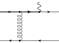
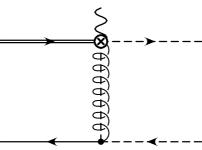
	$\longrightarrow$		$\longrightarrow$

Figure 1: Two-step matching procedure for a hard-scattering contribution. The dashed lines in the SCET_I diagram represent hard-collinear fields, those in the SCET_II four-quark operator denote collinear fields. In all cases, the heavy quark is depicted as a double line, and the wavy line represents the flavor-changing current.

In general, the $B$-type currents break the spin symmetries. When applied to form-factor matrix elements, the hard-collinear gluon emitted from the current is absorbed by the spectator quark, allowing the decay to proceed via the hard-scattering mechanism. Figure 1 illustrates the two-step matching of a typical hard-scattering amplitude. In the first step, the QCD current is matched onto a $B$-type SCET_I current. In the second step, the hard-collinear gluon is integrated out, and the hard-scattering amplitude is described in the final low-energy theory by non-local four-quark operators. Section 6 examines this SCET_II representation, where matrix elements take the form of the second, symmetry-breaking term in (1).

3.2 Matching calculations

We proceed to find the SCET_I representations of the QCD scalar, vector, and tensor currents

$$S=\bar{q}\,b\,,\qquad V^{\mu}=\bar{q}\,\gamma^{\mu}b\,,\qquad T^{\mu\nu}=(-i)\,\bar{q}\,\sigma^{\mu\nu}b=\bar{q}\,\gamma^{[\mu}\gamma^{\nu]}\,b\,.$$ (21)

The QCD operators $S$ and $T^{\mu\nu}$ require renormalization and are defined in the modified minimal subtraction ($\overline{\rm MS}$) scheme at a fixed scale $\mu_{\rm QCD}={\cal O}(m_{b})$. The $\mbox{SCET}_{\rm I}$ representations of these operators, evaluated at position $x=0$, are given by an expansion (summed over $i,j$)

$$\bar{q}\,\Gamma\,b \to \int ds\,\tilde{C}_{i}^{A}(s)\,J^{A}_{i}(s)+\frac{1}{2E}\int dr\,ds\,\tilde{C}^{B}_{j}(s,r)\,J^{B}_{j}(s,r)+\dots$$ (22)

$$= C^{A}_{i}(E)\,J^{A}_{i}(0)+\frac{1}{2E}\int du\,C^{B}_{j}(E,u)\,J^{B}_{j}(u)+\dots$$

with operators $J^{A}_{i}$, $J^{B}_{j}$ as determined in the previous section for the appropriate quantum numbers. We denote coefficient functions in position space with a tilde. In the second line, we have used translational invariance and defined the momentum-space coefficients (without a tilde) as

$$C^{A}_{i}(E) = \int ds\,e^{is\bar{n}\cdot P}\,\tilde{C}^{A}_{i}(s)\,,$$

$$C^{B}_{j}(E,u) = \int dr\,ds\,e^{i(us+\bar{u}r)\bar{n}\cdot P}\,\tilde{C}^{B}_{j}(s,r)\,.$$ (23)

Here $P=P_{\rm out}-P_{\rm in}$ is the total hard-collinear momentum of external states (strictly speaking this is a momentum operator), and $E=v\cdot P_{-}=(n\cdot v)(\bar{n}\cdot P)/2$. Reparameterization invariance ensures that the momentum-space coefficient functions depend on the combination $(n\cdot v)(\bar{n}\cdot P)=2E$, not $\bar{n}\cdot P$. The variable $u\in[0,1]$ is the fraction of the large momentum component $\bar{n}\cdot P$ carried by the fields in $\bar{\mathcal{X}}$ (the dressed outgoing hard-collinear quark field), and $\bar{u}\equiv 1-u$ is the corresponding momentum fraction carried by the fields in ${\mathcal{A}}_{\perp}$ (the dressed outgoing hard-collinear gluon field). The object $J^{B}_{j}(u)$ in (22) denotes the Fourier-transformed current operator

$$J_{j}^{B}(u)=\bar{n}\cdot P\int{ds\over 2\pi}\,e^{-iu\bar{n}\cdot Ps}\,J_{j}^{B}(s,0)\,.$$ (24)

Note that both $J_{i}^{A}(0)$ and $J_{j}^{B}(u)$ also depend on the large energy scale $E$ as well as on the renormalization scale $\mu$. These dependences will be suppressed for simplicity.

The matching conditions for the momentum-space Wilson coefficient functions $C_{i}^{A}$ and $C_{j}^{B}$ at tree level follow from an analysis of current matrix elements in QCD and SCET_I. The only subtlety is that a non-zero matching contribution is obtained from graphs where a hard-collinear gluon is emitted from the hard-collinear quark line. This might seem surprising at first sight, because the resulting propagator is close to the mass-shell. This contribution is present because two of the four components of the hard-collinear quark spinor are removed when QCD is matched onto SCET_I. To see how it arises, consider the following diagram:

= + (25)

$$\gamma_{\mu}\,\frac{1}{\hbox to0.0pt{\hskip 0.56917pt/\hss}{p}}\,\Gamma = \gamma_{\mu}\,\frac{\hbox to0.0pt{\hskip 0.56917pt/\hss}{n}}{2}\,\frac{1}{n\cdot p}\,\Gamma + \gamma_{\mu}\,\frac{\hbox to0.0pt{\hskip 0.56917pt/\hss}{\bar{n}}}{2}\,\frac{1}{\bar{n}\cdot p}\,\Gamma$$

For vanishing transverse momentum ($p_{\perp}=0$), the intermediate quark propagator takes the form shown in the second line. In the effective theory, the first term on the right hand side is represented by a graph where the gluon is emitted from a hard-collinear quark line. The second one, however, corresponds to a graph where the gluon is emitted from the $B$-type current, and contributes to the matching coefficient. Our tree-level results are given as follows.

Scalar current:

$$C^{A}_{S}=1\,,\qquad C^{B}_{S}=-1\,.$$ (26)

Vector current:

$$C^{A}_{V1} = 1\,,\qquad C^{A}_{V2,3}=0\,,$$

$$C^{B}_{V1} = 1\,,\qquad C^{B}_{V2}=-2\,,\qquad C^{B}_{V3}=-x\,,\qquad C^{B}_{V4}=0\,.$$ (27)

Tensor current:

$$C^{A}_{T1} = 1\,,\!\quad\qquad C^{A}_{T2,3,4}=0\,,$$

$$C^{B}_{T1} = -1\,,\qquad C^{B}_{T2}=-4\,,\qquad C^{B}_{T3}=-2x\,,\qquad C^{B}_{T4,5,6}=0\,,\qquad C^{B}_{T7}=-4x\,.$$ (28)

Here $x=2E/m_{b}$. Our tree-level matching coefficients agree with previous results, for $C_{i}^{A}$ in [1], and for $C_{j}^{B}$ in [4, 19]. 

Figure 2: One-loop QCD diagrams contributing to the matching calculation for the subleading scalar current. The external gluon can be attached at any of the places marked by a cross.

For the resummation of the leading logarithms, the tree-level Wilson coefficients are sufficient. However, for the physical value of the $b$-quark mass the one-loop matching corrections may turn out to be comparable to the effect of leading-order running. To address this question, we evaluate as an example the one-loop matching corrections for the scalar current. We calculate the decay of a $b$-quark to an energetic light quark and an energetic gluon at one-loop order. Throughout this paper we use dimensional regularization with $d=4-2\epsilon$ dimensions and employ the $\overline{\rm MS}$ scheme to remove ultra-violet (UV) singularities. We use the background-field method and perform the calculation in an arbitrary covariant gauge. The eight one-loop diagrams contributing to the matrix element are shown in Figure 2. Each diagram involves at least one heavy-quark propagator; diagrams involving only massless propagators vanish in dimensional regularization once the external lines are put on the mass shell. Note that there is again a contribution in Figure 2 corresponding to gluon emission from a nearly on-shell hard-collinear quark line, which is decomposed as in (25). To correctly identify the two parts of the QCD loop diagram, one first considers it for $p^{2}\neq 0$ and then expands around $p^{2}=0$. This expansion must be done before performing loop integrations. This ensures that all effective-theory loop diagrams vanish and only the hard part of the QCD diagram is left, which is exactly the part that has to be absorbed into the Wilson coefficients. We set all perpendicular components of the external momenta to zero and equate the effective-theory expression to the QCD result for the three-point function. Depending on the polarization of the background gluon field, we thus determine either the Wilson coefficient $C_{S}^{A}$ of the leading-order current operator (for an $A_{-}$ gluon), or the coefficient $C_{S}^{B}$ of the subleading current (for an $A_{\perp}$ gluon). After $\overline{\rm MS}$ subtractions, we obtain in the first case (again with $x=2E/m_{b}$)

$$C^{A}_{S}(E)=1+\frac{C_{F}\alpha_{s}}{4\pi}\left[-2\ln^{2}\frac{2E}{\mu}+5\ln\frac{2E}{\mu}+6\ln\frac{\mu_{\rm QCD}}{2E}+\frac{3-x}{1-x}\,\ln x-2\,\mbox{Li}_{2}(1-x)-\frac{\pi^{2}}{12}\right],$$ (29)

where $\alpha_{s}\equiv\alpha_{s}(\mu)$. The fact that this expression, which was extracted from a three-point function, agrees with the result obtained from the heavy-to-light two-point function [1] follows from invariance under collinear gauge transformations. Performing the calculation for the case of perpendicular gluon polarization, we obtain for the coefficient of the operator $J^{B}_{S}$

$$C^{B}_{S}(E,u) = -C_{S}^{A}(E)+\frac{C_{F}\alpha_{s}}{4\pi}\,\Bigg{\{}4\ln\frac{2E}{\mu}-4+\frac{2x}{1-x}\,\ln x$$ (30)

$$\mbox{}-\frac{x}{1-x\bar{u}}\left[1+\left(\frac{1}{1-x\bar{u}}+\frac{3-x}{1-x}\right)\ln(x\bar{u})\right]+\frac{2(2-x)}{1-x}\,\frac{\ln\bar{u}}{u}\Bigg{\}}$$

$$+ \left(C_{F}-\frac{C_{A}}{2}\right)\frac{\alpha_{s}}{4\pi}\,\Bigg{\{}\left(2\ln\frac{2E}{\mu}-1+\ln u\right)\frac{2\ln u}{\bar{u}}+\frac{2x}{1-x\bar{u}}\,\ln(x\bar{u})-\frac{2\ln\bar{u}}{u}$$

$$\mbox{}+\frac{2}{xu\bar{u}}\left[(1-xu)\,\Big{[}{\rm Li}_{2}(1-x)-{\rm Li}_{2}(1-xu)\Big{]}-{\rm Li}_{2}(1-x\bar{u})+\frac{\pi^{2}}{6}\right]\Bigg{\}}\,,$$

where $u$ corresponds to the fraction of the longitudinal hard-collinear momentum carried by the final-state quark. We note that at the endpoints, $C_{S}^{B}$ diverges only logarithmically: $C_{S}^{B}\sim\ln^{2}u$ at $u=0$ and $C_{S}^{B}\sim\ln\bar{u}$ at $\bar{u}=0$. Also, despite appearances, there is no singularity at $x=1$ or $x=1/\bar{u}$. The scale dependence of $C_{S}^{B}$ agrees with a direct analysis of operator renormalization given in the following section. We postpone a detailed discussion on the relative importance of matching and RG running until Section 5, when a solution to the RG equations is at hand.

As a final remark before ending this section, we note that the scalar current is not an independent operator but can be related to the vector current using the equation of motion for the quark fields, $i\partial_{\nu}V^{\nu}=\overline{m}_{b}(\mu_{\rm QCD})\,S(\mu_{\rm QCD})$, where $S(\mu_{\rm QCD})$ denotes the scalar QCD current in (21) renormalized at scale $\mu_{\rm QCD}$, and $\overline{m}_{b}(\mu_{\rm QCD})$ is the running $b$-quark mass, both defined in the $\overline{\rm MS}$ scheme. Applying this identity to (22), it follows that to all orders in $\alpha_{s}$ and at leading order in $\Lambda_{\rm QCD}/m_{b}$

$$C^{A}_{V1}+\left(1-{E\over m_{b}}\right)C^{A}_{V2}+C^{A}_{V3} = \frac{\overline{m}_{b}(\mu_{\rm QCD})}{m_{b}}\,C^{A}_{S}\,,$$

$$C^{B}_{V1}+\left(1-{E\over m_{b}}\right)C^{B}_{V2}+C^{B}_{V3} = \frac{\overline{m}_{b}(\mu_{\rm QCD})}{m_{b}}\,C^{B}_{S}\,,$$ (31)

where at this order there is no difference between the meson mass $m_{B}$ and the $b$-quark pole mass $m_{b}$. It is readily seen from (26) and (3.2) that these relations hold at tree level. At one-loop order

$$\frac{\overline{m}_{b}(\mu_{\rm QCD})}{m_{b}}=1+{C_{F}\alpha_{s}\over 4\pi}\left(6\ln{m_{b}\over\mu_{\rm QCD}}-4\right).$$ (32)

Note that the dependence on the scale $\mu_{\rm QCD}$ cancels between the running mass $\overline{m}_{b}(\mu_{\rm QCD})$ and the scalar coefficients $C_{S}^{A}$ and $C_{S}^{B}$ on the right-hand side of the relations in (3.2). The first of these relations can be verified to hold at one-loop order using the results of [1]. In Section 7, we will use these results to deduce the one-loop matching coefficients relevant to the vector form factor $F_{0}(q^{2})$, using only scalar-current matching calculations.

4 Anomalous dimensions

The matching results derived in the previous section can be trusted at a high renormalization point $\mu=\mu_{h}\sim 2E$, at which the Wilson coefficients are free of large logarithms and so can be reliably computed using fixed-order perturbation theory. In order to evolve the coefficients down to lower values of $\mu$, one needs to solve the RG equation for the SCET_I current operators.

The currents $J_{i}^{A}$ and $J_{j}^{B}$ do not mix under renormalization. To see this, we first note that the operators $J_{j}^{B}$ cannot mix into $J_{i}^{A}$, as they are of higher order in power counting than the leading terms of $J_{i}^{A}$. In principle, the operators $J_{i}^{A}$ could mix into $J_{j}^{B}$ via time-ordered products of either the leading terms of $J_{i}^{A}$ with the subleading SCET_I Lagrangian, or the subleading terms of $J_{i}^{A}$ with the leading SCET_I Lagrangian. However, when $v_{\perp}^{\mu}=0$, in both cases the resulting time-ordered products have a structure different from the $J_{j}^{B}$ operators, containing additional perpendicular partial derivatives acting on hard-collinear fields. Finally, the various $J^{A}_{i}$ operators do not mix among themselves, since time-ordered products with the SCET_I Lagrangian cannot mix the different Dirac structures appearing in their definition. As a result, the effective-theory currents obey the integro-differential RG equations (summation over $k$ is understood in the second equation)

$${d\over d\ln\mu}\,J_{i}^{A}(0) = -\gamma^{A}\,J_{i}^{A}(0)\,,$$

$${d\over d\ln\mu}\,J_{j}^{B}(u) = -\int_{0}^{1}\!dv\,\gamma^{B}_{jk}(u,v)\,J_{k}^{B}(v)\,,$$ (33)

and the corresponding momentum-space Wilson coefficients satisfy the equations

$${d\over d\ln\mu}\,C_{i}^{A}(E) = \gamma^{A}\,C_{i}^{A}(E)\,,$$

$${d\over d\ln\mu}\,C_{j}^{B}(E,v) = \int_{0}^{1}\!du\,\gamma^{B}_{kj}(u,v)\,C_{k}^{B}(E,u)\,.$$ (34)

The anomalous dimensions $\gamma^{A}$ and $\gamma_{jk}^{B}$ are calculated by isolating the UV divergences in SCET_I loop diagrams. The one-loop expression for $\gamma^{A}$ has been calculated previously [1], with the result

$$\gamma^{A}=-\Gamma_{\rm cusp}(\alpha_{s})\,\ln{\mu\over 2E}+\tilde{\gamma}(\alpha_{s})={C_{F}\alpha_{s}\over\pi}\left(-\ln{\mu\over 2E}-{5\over 4}\right)+{\cal O}(\alpha_{s}^{2})\,.$$ (35)

In [20] it was argued that the first equality in (35) is valid to all orders in $\alpha_{s}$. The appearance of $\ln\mu$ in the anomalous dimension is explained by the theory of light-like Wilson loops with cusps. Only a single logarithm appears at any order in the strong coupling, with a coefficient governed by the universal cusp anomalous dimension $\Gamma_{\rm cusp}$ [21].

Unlike the situation for the $A$-type operators, the anomalous dimensions of the $B$-type currents depend on the specific Dirac structure, and there is non-trivial operator mixing. The renormalization properties of all $B$-type operators can be discussed by defining two operators

$${\mathcal{J}}_{1}(s)=\bar{\mathcal{X}}(s\bar{n})\,{\mathcal{A}}_{\perp\mu}(0)\,\Gamma_{\perp}^{\mu}\,h(0)\,,\qquad{\mathcal{J}}_{2}(s)=\bar{\mathcal{X}}(s\bar{n})\,{\mathcal{A}}_{\perp\mu}(0)\,\gamma_{\perp}^{\mu}\gamma_{\perp\nu}\,\Gamma_{\perp}^{\nu}\,h(0)\,,$$ (36)

and their Fourier transforms as defined in (24). The Dirac structure $\Gamma_{\perp}^{\mu}$ is determined by the specific current under consideration. It follows from the Feynman rules of SCET_I and the projection properties of the two-component spinor ${\mathcal{X}}$ that the two operators ${\mathcal{J}}_{i}$ close under renormalization. Defining renormalization constants via ${\mathcal{J}}_{i}^{\rm ren}=Z_{ij}\,{\mathcal{J}}_{j}^{\rm bare}$, we obtain

$$\mbox{\boldmath$Z$\unboldmath}=\left(\begin{array}[]{cc}Z_{11}&Z_{12}\\ 0&~{}~{}Z_{11}+2(1-\epsilon)Z_{12}\end{array}\right)_{\rm\!\!poles},$$ (37)

where, in the $\overline{\rm MS}$ scheme, it is understood that only pole terms in the dimensional regulator $\epsilon=2-d/2$ are kept in $\mbox{\boldmath$Z$\unboldmath}-\mbox{\boldmath$1$\unboldmath}$. We define two anomalous-dimension functions

$$\gamma_{1}=2\alpha_{s}\,\frac{\partial}{\partial\alpha_{s}}\,Z^{(1)}_{11}\,,\qquad\gamma_{2}=2\alpha_{s}\,\frac{\partial}{\partial\alpha_{s}}\,Z^{(1)}_{12}\,,$$ (38)

where $\mbox{\boldmath$Z$\unboldmath}^{(1)}$ is the coefficient of the $1/\epsilon$ pole in $Z$. Then, at one-loop order, the corresponding anomalous dimension matrix determining the running of the currents ${\mathcal{J}}_{i}$ reads

$$\mbox{\boldmath$\gamma$\unboldmath}_{\rm 1-loop}=\left(\begin{array}[]{cc}\gamma_{1}&\gamma_{2}\\ 0&~{}~{}\gamma_{1}+2\gamma_{2}\end{array}\right).$$ (39)

At higher order, the ${\cal O}(\epsilon)$ terms arising from the Dirac algebra have a non-trivial effect on the anomalous dimensions, as discussed in [22].

In terms of these functions, the anomalous dimension of the scalar current is (from now on all results refer to the one-loop approximation)

$$\gamma^{B}_{S}=\gamma_{1}+2\gamma_{2}\,.$$ (40)

For the vector current, we find the $4\times 4$ anomalous-dimension matrix

$$\mbox{\boldmath$\gamma$\unboldmath}^{B}_{V}=\left(\begin{array}[]{ccc|c}\gamma_{1}+2\gamma_{2}&0&0&0\\ 0&\gamma_{1}+2\gamma_{2}&0&0\\ 0&0&\gamma_{1}+2\gamma_{2}&0\\ \hline\cr\gamma_{2}&0&-\gamma_{2}&\gamma_{1}\end{array}\right).$$ (41)

The operators $J_{V1,2,3}^{B}$ are multiplicatively renormalized with anomalous dimension $\gamma_{1}+2\gamma_{2}$, whereas the operator $J_{V4}^{B}$ mixes with $J_{V1}^{B}$ and $J_{V3}^{B}$. For the form factor analysis, it will be convenient to work with the linear combinations

$$J_{V1}^{B^{\prime}\mu} = J_{V1}^{B\,\mu}-J_{V3}^{B\,\mu}=\bar{\mathcal{X}}(s\bar{n})\,\hbox to0.0pt{\hskip 2.27626pt/\hss}{{\mathcal{A}}}_{\perp}(r\bar{n})\,\gamma_{\perp}^{\mu}\,h(0)\,,$$

$$J_{V2}^{B^{\prime}\mu} = J_{V2}^{B\,\mu}=\bar{\mathcal{X}}(s\bar{n})\,\hbox to0.0pt{\hskip 2.27626pt/\hss}{{\mathcal{A}}}_{\perp}(r\bar{n})\,v^{\mu}\,h(0)\,,$$

$$J_{V3}^{B^{\prime}\mu} = J_{V3}^{B\,\mu}=\bar{\mathcal{X}}(s\bar{n})\,\hbox to0.0pt{\hskip 2.27626pt/\hss}{{\mathcal{A}}}_{\perp}(r\bar{n})\,\frac{n^{\mu}}{n\cdot v}\,h(0)\,,$$

$$J_{V4}^{B^{\prime}\mu} = 2J_{V4}^{B\,\mu}-J_{V1}^{B\,\mu}+J_{V3}^{B\,\mu}=\bar{\mathcal{X}}(s\bar{n})\,\gamma_{\perp}^{\mu}\,\hbox to0.0pt{\hskip 2.27626pt/\hss}{{\mathcal{A}}}_{\perp}(r\bar{n})\,h(0)\,,$$ (42)

which are multiplicatively renormalized. $J_{V1,2,3}^{B^{\prime}}$ have anomalous dimension $\gamma_{1}+2\gamma_{2}$, while $J_{V4}^{B^{\prime}}$ has anomalous dimension $\gamma_{1}$. The corresponding combinations of Wilson coefficients, which are multiplicatively renormalized with the same anomalous dimensions as the respective currents $J_{j}^{B^{\prime}}$, read

$$C_{V1}^{B^{\prime}} = C_{V1}^{B}+\frac{1}{2}\,C_{V4}^{B}\,,\qquad C_{V2}^{B^{\prime}}=C_{V2}^{B}\,,\qquad C_{V3}^{B^{\prime}}=C_{V3}^{B}+C_{V1}^{B}\,,$$

$$C_{V4}^{B^{\prime}} = \frac{1}{2}\,C_{V4}^{B}\,.$$ (43)

Similarly, for the tensor current we find that the operators $J_{T1,2,3,4}^{B}$ are multiplicatively renormalized with anomalous dimension $\gamma_{1}+2\gamma_{2}$, whereas the operators $J_{T5,6,7}^{B}$ mix with $J_{T1,2,3,4}^{B}$. As in the vector case, it will be convenient to change the operator basis, defining

$$J_{T1}^{B^{\prime}\mu\nu} = J_{T1}^{B\,\mu\nu}+2J_{T3}^{B\,\mu\nu}-2J_{T4}^{B\,\mu\nu}=\bar{\mathcal{X}}(s\bar{n})\,\hbox to0.0pt{\hskip 2.27626pt/\hss}{{\mathcal{A}}}_{\perp}(r\bar{n})\,\gamma_{\perp}^{[\mu}\gamma_{\perp}^{\nu]}\,h(0)\,,$$

$$J_{T2}^{B^{\prime}\mu\nu} = J_{T2}^{B\,\mu\nu}+J_{T4}^{B\,\mu\nu}=\bar{\mathcal{X}}(s\bar{n})\,\hbox to0.0pt{\hskip 2.27626pt/\hss}{{\mathcal{A}}}_{\perp}(r\bar{n})\,v^{[\mu}\gamma_{\perp}^{\nu]}\,h(0)\,,$$

$$J_{T3}^{B^{\prime}\mu\nu} = J_{T3}^{B\,\mu\nu}=\bar{\mathcal{X}}(s\bar{n})\,\hbox to0.0pt{\hskip 2.27626pt/\hss}{{\mathcal{A}}}_{\perp}(r\bar{n})\,{n^{[\mu}\gamma_{\perp}^{\nu]}\over n\cdot v}\,h(0)\,,$$

$$J_{T4}^{B^{\prime}\mu\nu} = J_{T4}^{B\,\mu\nu}=\bar{\mathcal{X}}(s\bar{n})\,\hbox to0.0pt{\hskip 2.27626pt/\hss}{{\mathcal{A}}}_{\perp}(r\bar{n})\,{n^{[\mu}v^{\nu]}\over n\cdot v}\,h(0)\,,$$

$$J_{T5}^{B^{\prime}\mu\nu} = -2J_{T5}^{B\,\mu\nu}+J_{T1}^{B\,\mu\nu}+2J_{T3}^{B\,\mu\nu}-2J_{T4}^{B\,\mu\nu}+2J_{T7}^{B\,\mu\nu}=\bar{\mathcal{X}}(s\bar{n})\,{\mathcal{A}}_{\perp\alpha}(r\bar{n})\,\gamma_{\perp}^{[\alpha}\gamma_{\perp}^{\mu}\gamma_{\perp}^{\nu]}\,h(0)\,,$$

$$J_{T6}^{B^{\prime}\mu\nu} = -2J_{T6}^{B\,\mu\nu}-J_{T2}^{B\,\mu\nu}-J_{T4}^{B\,\mu\nu}=\bar{\mathcal{X}}(s\bar{n})\,v^{[\mu}\gamma_{\perp}^{\nu]}\,\hbox to0.0pt{\hskip 2.27626pt/\hss}{{\mathcal{A}}}_{\perp}(r\bar{n})\,h(0)\,,$$

$$J_{T7}^{B^{\prime}\mu\nu} = -2J_{T7}^{B\,\mu\nu}-J_{T3}^{B\,\mu\nu}=\bar{\mathcal{X}}(s\bar{n})\,\frac{n^{[\mu}\gamma_{\perp}^{\nu]}}{n\cdot v}\,\hbox to0.0pt{\hskip 2.27626pt/\hss}{{\mathcal{A}}}_{\perp}(r\bar{n})\,h(0)\,.$$ (44)

These operators are multiplicatively renormalized, $J_{T1,2,3,4}^{B^{\prime}}$ with anomalous dimension $\gamma_{1}+2\gamma_{2}$, and $J_{T5,6,7}^{B^{\prime}}$ with anomalous dimension $\gamma_{1}$. The corresponding combinations of Wilson coefficients are

$$C_{T1}^{B^{\prime}} = C_{T1}^{B}+\frac{1}{2}\,C_{T5}^{B}\,,\qquad C_{T2}^{B^{\prime}}=C_{T2}^{B}-\frac{1}{2}\,C_{T6}^{B}\,,\qquad C_{T3}^{B^{\prime}}=C_{T3}^{B}-2C_{T1}^{B}-\frac{1}{2}\,C_{T5}^{B}-\frac{1}{2}\,C_{T7}^{B}\,,$$

$$\hskip 94.46335ptC_{T4}^{B^{\prime}}=C_{T4}^{B}+2C_{T1}^{B}-C_{T2}^{B}\,,$$

$$C_{T5}^{B^{\prime}} = -\frac{1}{2}\,C_{T5}^{B}\,,\qquad C_{T6}^{B^{\prime}}=-\frac{1}{2}\,C_{T6}^{B}\,,\qquad C_{T7}^{B^{\prime}}=-\frac{1}{2}\,C_{T7}^{B}-\frac{1}{2}\,C_{T5}^{B}\,.$$ (45)

Note that the tree-level matrix elements of the “evanescent” operator $J_{T5}^{B^{\prime}}$ vanish in $d=4$ dimensions, and after additional finite renormalizations the same is true once loop corrections are included. This operator will not be relevant for our leading-order analysis, but it would enter a next-to-leading order calculation employing dimensional regularization. We will mention evanescent operators again in Section 6, when we discuss the basis of SCET_II four-quark operators relevant to the hard-scattering contributions.

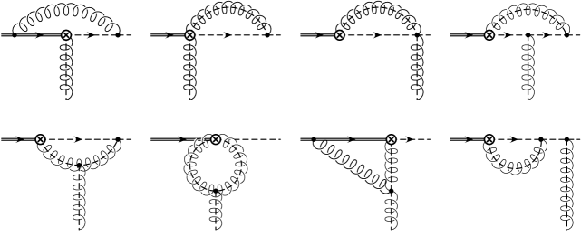
Figure 3: $\mbox{SCET}_{\rm I}$ graphs contributing to the anomalous dimensions of the subleading heavy-collinear currents $J_{j}^{B}$, represented by a crossed circle. Full lines denote soft fields, dashed lines hard-collinear fields.

To calculate the one-loop anomalous dimensions, we evaluate the UV poles of the diagrams shown in Figure 3 in dimensional regularization, treating the external gluon as a background field. The resulting expressions for the integral operators $\gamma_{1}$ and $\gamma_{2}$ can be written as

$$\gamma_{1}(u,v) = u\,V_{1}(u,v)+\delta(u-v)\,W(E,u)\,,$$

$$2\gamma_{2}(u,v) = u\,V_{2}(u,v)\,,$$ (46)

where

$$V_{1}(u,v) = \left(C_{F}-\frac{C_{A}}{2}\right){\alpha_{s}\over\pi}\left(-{\theta(1-u-v)\over\bar{u}\bar{v}}\right)$$

$$\mbox{}-{C_{A}\over 2}{\alpha_{s}\over\pi}\left\{{1\over uv}\left[u\,{\theta(v-u)\over(v-u)}+v\,{\theta(u-v)\over(u-v)}\right]_{+}-{\theta(v-u)\over v\bar{u}}-{\theta(u-v)\over u\bar{v}}\right\},$$

$$V_{2}(u,v) = \left(C_{F}-\frac{C_{A}}{2}\right){\alpha_{s}\over\pi}\left[\left(1+{1\over\bar{u}}+{1\over\bar{v}}\right)\theta(1-u-v)+{\bar{u}\bar{v}\over uv}\,\theta(u+v-1)\right]$$

$$\mbox{}-{C_{A}\over 2}{\alpha_{s}\over\pi}\left[\frac{\bar{u}}{u}\left(1+\frac{1}{\bar{v}}\right)\theta(u-v)+\frac{\bar{v}}{v}\left(1+\frac{1}{\bar{u}}\right)\theta(v-u)\right],$$

$$W(E,u) = C_{F}{\alpha_{s}\over\pi}\left(-\ln{\mu\over 2E}-{5\over 4}+\ln u\right)-{C_{A}\over 2}{\alpha_{s}\over\pi}\left(\ln\frac{u}{\bar{u}}-1\right).$$ (47)

For symmetric functions $g(u,v)$ the plus distribution is defined to act on test functions $f(v)$ as

$$\int dv\,[g(u,v)]_{+}\,f(v)=\int dv\,g(u,v)\,\big{[}f(v)-f(u)\big{]}\,.$$ (48)

It is remarkable that the functions $V_{i}(u,v)$ are symmetric in their arguments. This fact is not accidental, but can be traced back to a residual conformal symmetry in the effective theory when interactions with the soft heavy quark are ignored. Also, since soft gluons are unable to change the large component of hard-collinear momenta, the one-loop conformal-symmetry breaking term $\delta(u-v)W(E,u)$ is local with respect to $u$. Details of the conformal-symmetry arguments will be presented in Section 5.3.

From (4), it follows that the evolution equation for the current eigenvectors $J_{j}^{B^{\prime}}$ takes the form

$${d\over d\ln{\mu}}\,J_{j}^{B^{\prime}}(u)=-\int_{0}^{1}\!dv\,u\,V_{\Gamma}(u,v)\,J_{j}^{B^{\prime}}(v)-W(E,u)\,J_{j}^{B^{\prime}}(u)\,,$$ (49)

where $V_{\Gamma}$ is a linear combination of $V_{1}$ and $V_{2}$ determined by the anomalous dimension of the operator $J_{j}^{B^{\prime}}$. For reasons that will become clear later, we use the notation $\Gamma=\,\parallel,\perp$ and denote $V_{\parallel}=V_{1}+V_{2}$ for operators with anomalous dimension $\gamma_{1}+2\gamma_{2}$, and $V_{\perp}=V_{1}$ for operators with anomalous dimension $\gamma_{1}$. The corresponding equation for the eigenvectors $C_{j}^{B^{\prime}}$ of Wilson coefficients reads

$${d\over d\ln\mu}\,C_{j}^{B^{\prime}}(E,v)=\int_{0}^{1}\!du\,u\,V_{\Gamma}(u,v)\,C_{j}^{B^{\prime}}(E,u)+W(E,v)\,C_{j}^{B^{\prime}}(E,v)\,.$$ (50)

To gain more insight into the structure of the conformal-symmetry breaking term $W(E,u)$, we may consider the field redefinitions [2, 15]

$$\xi_{hc}(x)=S_{n}(x_{-})\,\xi_{hc}^{(0)}(x)\,,\qquad A_{hc}^{\mu}(x)=S_{n}(x_{-})\,A_{hc}^{(0)\mu}(x)\,S_{n}^{\dagger}(x_{-})\,,\qquad h(x)=S_{v}(x)\,h^{(0)}(x)\,,$$ (51)

which decouple soft gluons from the leading-order hard-collinear and heavy-quark Lagrangians. Here $S_{n}$ and $S_{v}$ are soft Wilson lines in the $n$ and $v$ directions, respectively. From (7), it follows that in terms of the new fields the $B$-type operators take the form

$$J^{B}_{j}(s,r)=\bar{\mathcal{X}}^{(0)}(s\bar{n})\,{\mathcal{A}}_{\perp\mu}^{(0)}(r\bar{n})\,\Gamma_{\perp}^{\mu}\big{[}S_{n}^{\dagger}\,S_{v}\big{]}(0)\,h^{(0)}(0)\,.$$ (52)

The combination $[S_{n}^{\dagger}\,S_{v}](0)$ represents a closed loop with a cusp at $x=0$ formed by two Wilson lines in the $v$ and $n$ directions. The anomalous dimension of this object is given by the universal cusp anomalous dimension times a logarithm of the soft scale [21]. After adding a contribution from the hard-collinear sector necessary to eliminate the dependence on the infra-red regulator $(-p_{hc}^{2})$ (c.f. [15, 23],), the result is

$$\Gamma_{\rm cusp}\left[\ln{2v\cdot p_{hc}\,\mu\over(-p_{hc}^{2})}+\ln{(-p_{hc}^{2})\over\mu^{2}}\right]=\Gamma_{\rm cusp}\,\ln{2v\cdot p_{hc}\over\mu}\,,$$ (53)

with $p_{hc}$ a hard-collinear momentum. From these considerations, we conclude that to all orders in perturbation theory

$$W(E,u)=-\Gamma_{\rm cusp}(\alpha_{s})\,\ln{\mu\over 2E}+w(u,\alpha_{s}),$$ (54)

with the one-loop expression for $w$ determined from (4).

5 Renormalization-group evolution in SCET_I

The anomalous dimensions obtained in the previous section allow us to solve the RG evolution equations (49) and (50) at leading order in RG-improved perturbation theory. At this order the leading double and single logarithmic contributions are resummed to all orders in perturbation theory. Technically, this means that one must compute the matching coefficients at tree level, the anomalous dimension kernels $V_{i}(u,v)$ at one-loop order, and the cusp anomalous dimension entering the function $W(E,u)$ at two-loop order. In practice, one wants to impose matching conditions for the coefficient functions $C_{j}^{B^{\prime}}$ at a high scale $\mu_{h}\sim 2E$ and then evolve the result down to an intermediate scale $\mu_{i}\sim\sqrt{2E\Lambda_{\rm QCD}}$, at which SCET_I is matched onto the low-energy effective theory SCET_II. While the integro-differential evolution equations can be solved numerically, we find it instructive to also discuss a formal analytic solution to these equations.

5.1 Eigenfunctions and eigenvalues of the evolution operator

It will be convenient to rewrite (49) and (50) in the somewhat obscure form

$${d\over d\ln{\mu}}\,{J_{j}^{B^{\prime}}(u)\over u\bar{u}} = -\int_{0}^{1}\!dv\,v\bar{v}^{2}\,{V_{\Gamma}(u,v)\over\bar{u}\bar{v}}\,{J_{j}^{B^{\prime}}(v)\over v\bar{v}}-W(E,u)\,{J_{j}^{B^{\prime}}(u)\over u\bar{u}}\,,$$

$${d\over d\ln{\mu}}\,{C_{j}^{B^{\prime}}(E,u)\over\bar{u}} = \int_{0}^{1}\!dv\,v\bar{v}^{2}\,{V_{\Gamma}(v,u)\over\bar{u}\bar{v}}\,{C_{j}^{B^{\prime}}(E,v)\over\bar{v}}+W(E,u)\,{C_{j}^{B^{\prime}}(E,u)\over\bar{u}}\,.$$ (55)

Because of the symmetry property $V_{i}(u,v)=V_{i}(v,u)$, it follows that the operator eigenfunctions $[J_{n}^{B^{\prime}}(u)/u\bar{u}]$ have the same form as the coefficient eigenfunctions $[C_{n}^{B^{\prime}}(u)/\bar{u}]$, but come with eigenvalues of the opposite sign. We consider first the hypothetical case where $W(E,u)=0$ and focus on the non-diagonal terms in the evolution kernels, $V_{i}(u,v)$ with $i=1,2$. We will show that the general solution to the eigenvalue equation

$$\int_{0}^{1}\!du\,u\bar{u}^{2}\,{V_{i}(u,v)\over\bar{u}\bar{v}}\,\psi_{n}(u)=\lambda_{i,n}\,\psi_{n}(v)$$ (56)

is given by

$$\psi_{n}(u)=\sqrt{2(n+2)(n+3)\over n+1}\,P_{n}^{(2,1)}(2u-1)\,,$$ (57)

where $P_{n}^{(2,1)}$ are Jacobi (hyper-geometric) polynomials, and the eigenfunctions $\psi_{n}$ are normalized according to

$$\langle\psi_{n}|\psi_{m}\rangle\equiv\int_{0}^{1}\!du\,u\bar{u}^{2}\,\psi_{n}(u)\,\psi_{m}(u)=\delta_{nm}\,.$$ (58)

The eigenvalues for the kernels $V_{1}$ and $V_{2}$ may be expressed in the closed form

$$\lambda_{1,n} = \left(C_{F}-\frac{C_{A}}{2}\right){\alpha_{s}\over\pi}\,{(-1)^{n+1}\over n+2}-{C_{A}\over 2}\,{\alpha_{s}\over\pi}\left(1-2H_{n+1}-{1\over n+2}\right),$$

$$\lambda_{2,n} = \left(C_{F}-\frac{C_{A}}{2}\right){\alpha_{s}\over\pi}\,{(-1)^{n}(n^{2}+4n+5)\over(n+1)(n+2)(n+3)}-{C_{A}\over 2}\,{\alpha_{s}\over\pi}\,{2\over(n+1)(n+3)}\,,$$ (59)

where $H_{n}=\sum_{m=1}^{n}1/m$ are the harmonic numbers. Using the solution to the eigenvalue equation for $V_{i}$, we then present a formal algebraic solution to the evolution equation for the SCET_I coefficient functions.

Let us now prove the statements just made. We proceed along lines similar to the diagonalization of the evolution kernel for the pion LCDA, as analyzed in [24] (see in particular Appendix D). From the eigenvalue equation (56) and the symmetry of $V_{i}(u,v)$ it follows that eigenfunctions belonging to different eigenvalues must be orthogonal in the measure $u\bar{u}^{2}\,du$ on the interval $0\leq u\leq 1$, as shown in (58). To show that the eigenfunctions take the form (57), we consider the integrals

$${\cal I}_{i,n}(v)=\int_{0}^{1}\!du\,u\bar{u}^{2}\,{V_{i}(u,v)\over\bar{u}\bar{v}}\,(2u-1)^{n}\,.$$ (60)

We will show below that ${\cal I}_{i,n}(v)$ is a polynomial in $(2v-1)$ of degree $n$. Hence, in operator notation, with $\langle u|n\rangle\equiv(2u-1)^{n}$ and $\langle u|V_{i}|n\rangle\equiv{\cal I}_{i,n}(u)$, we have

$$V_{i}|n\rangle=\sum_{m=0}^{n}(V_{i})_{mn}|m\rangle$$ (61)

with $(V_{i})_{mn}=0$ for $m>n$. In particular, $|0\rangle$ is an eigenfunction with eigenvalue $(V_{i})_{00}$. By induction, for each $n\geq 1$ there is a corresponding eigenvalue given by the diagonal matrix element $(V_{i})_{nn}$ with eigenfunction proportional to the linear combination of $|0\rangle,\dots,|n\rangle$ that is orthogonal to each of $|0\rangle,\dots,|n-1\rangle$. The result (57) follows since the Jacobi polynomials $P_{n}^{(2,1)}(2u-1)$ form the unique extension of the constant function to a basis of orthogonal polynomials with measure $u\bar{u}^{2}\,du$ on the unit interval. As a byproduct of this analysis, the coefficient of $(2v-1)^{n}$ in the expansion of ${\cal I}_{i,n}(v)$ is identified with the $n$-th eigenvalue $\lambda_{i,n}$.

To evaluate ${\cal I}_{i,n}$, it is convenient to introduce new variables $x=2u-1$ and $y=2v-1$. The resulting integrals yield

$${\cal I}_{1,n} = \left(C_{F}-\frac{C_{A}}{2}\right){\alpha_{s}\over\pi}\,(-1)^{n+1}\sum_{m=0}^{n}{m+1\over(n+1)(n+2)}\,y^{m}$$

$$\mbox{}-{C_{A}\over 2}\,{\alpha_{s}\over\pi}\left[(1-2H_{n+1})\,y^{n}+\sum_{m=0}^{n-1}{\left[1+(-1)^{n-m}\right]\,(m+1)\over(n-m)(n+1)}\,y^{m}-\!\sum_{m=0}^{n}{m+1\over(n+1)(n+2)}\,y^{m}\right],$$

$${\cal I}_{2,n} = \left(C_{F}-\frac{C_{A}}{2}\right){\alpha_{s}\over\pi}\,{(-1)^{n}\over 2(n+1)(n+2)(n+3)}\sum_{m=0}^{n}\left[(-1)^{n-m}+9+4(n+m)+2nm\right]y^{m}$$ (62)

$$\mbox{}-{C_{A}\over 2}\,{\alpha_{s}\over\pi}\,{1\over 2(n+1)(n+2)(n+3)}\sum_{m=0}^{n}\left[(5+2n)(-1)^{n-m}+3+2m\right]y^{m}\,.$$

Inspection of these results shows that the coefficient of $y^{m}$ in ${\cal I}_{i,n}$ indeed vanishes for $m>n$, while the coefficient of $y^{n}$ gives the eigenvalues (5.1).

5.2 Solution to the evolution equation

Due to the presence of the conformal-symmetry breaking term $W(E,u)$, the eigenfunctions of the full anomalous-dimension operators $\gamma_{1}+2\gamma_{2}$ and $\gamma_{1}$ cannot be written in closed form. We will now show how a formal algebraic solution can be obtained. We begin by isolating the strong $\mu$ dependence of the coefficient functions due to $\Gamma_{\rm cusp}$, writing the solution to the evolution equation (5.1) as

$$C_{j}^{B^{\prime}}(E,u,\mu)=\left({2E\over\mu_{h}}\right)^{a(\mu_{h},\mu)}e^{S(\mu_{h},\mu)}\int_{0}^{1}dv\,U_{\Gamma}(u,v,\mu_{h},\mu)\,C_{j}^{B^{\prime}}(E,v,\mu_{h})\,,$$ (63)

where

$$S(\mu_{1},\mu_{2})=-\int_{\alpha_{s}(\mu_{1})}^{\alpha_{s}(\mu_{2})}{d\alpha\over\beta(\alpha)}\,\Gamma_{\rm cusp}(\alpha)\int_{\alpha_{s}(\mu_{1})}^{\alpha}{d\alpha^{\prime}\over\beta(\alpha^{\prime})}\,,$$ (64)

with $\beta(\alpha_{s})\equiv d\alpha_{s}/d\ln\mu$, is a universal Sudakov factor, and

$$a(\mu_{1},\mu_{2})=\int_{\alpha_{s}(\mu_{1})}^{\alpha_{s}(\mu_{2})}{d\alpha\over\beta(\alpha)}\,\Gamma_{\rm cusp}(\alpha)\,.$$ (65)

Note that $S(\mu_{1},\mu_{2})$ is negative, since $\Gamma_{\rm cusp}(\alpha_{s})\geq 0$ [25]. At leading order in RG-improved perturbation theory one finds [20]

$$S(\mu_{h},\mu) = \frac{\Gamma_{0}}{4\beta_{0}^{2}}\left[\frac{4\pi}{\alpha_{s}(\mu_{h})}\left(1-\frac{1}{r_{1}}-\ln r_{1}\right)+\frac{\beta_{1}}{2\beta_{0}}\,\ln^{2}r_{1}-\left(\frac{\Gamma_{1}}{\Gamma_{0}}-\frac{\beta_{1}}{\beta_{0}}\right)(r_{1}-1-\ln r_{1})\right],$$

$$a(\mu_{h},\mu) = -\frac{\Gamma_{0}}{2\beta_{0}}\,\ln r_{1}\,,$$ (66)

where $r_{1}=\alpha_{s}(\mu)/\alpha_{s}(\mu_{h})\geq 1$. The relevant RG coefficients arising in the perturbative expansion of the cusp anomalous dimension and the $\beta$ function,

$$\beta(\alpha_{s})=-2\alpha_{s}\sum_{n=0}^{\infty}\beta_{n}\left({\alpha_{s}\over 4\pi}\right)^{n+1},\qquad\Gamma_{\rm cusp}(\alpha_{s})=\sum_{n=0}^{\infty}\Gamma_{n}\left({\alpha_{s}\over 4\pi}\right)^{n+1},$$ (67)

are $\Gamma_{0}=4C_{F}$, $\Gamma_{1}=4C_{F}\,[({67\over 9}-{\pi^{2}\over 3})\,C_{A}-{20\over 9}\,T_{F}n_{f}]$, and $\beta_{0}={11\over 3}\,C_{A}-{4\over 3}\,T_{F}n_{f}$, $\beta_{1}={34\over 3}\,C_{A}^{2}-{20\over 3}\,C_{A}T_{F}n_{f}-4C_{F}T_{F}n_{f}$. We take $n_{f}=4$ as the number of light quark flavors, even at low renormalization scales.

The remaining evolution is governed by a function $U_{\Gamma}(u,v,\mu_{h},\mu)$ with initial condition $U_{\Gamma}(u,v,\mu_{h},\mu_{h})=\delta(u-v)$ at the high-energy matching scale $\mu=\mu_{h}$. From (5.1) we find the corresponding RG equation

$${d\over d\ln\mu}\,\frac{U_{\Gamma}(u,v,\mu_{h},\mu)}{\bar{u}}=\int_{0}^{1}\!dy\,y\bar{y}^{2}\,\frac{V_{\Gamma}(y,u)}{\bar{y}\bar{u}}\,\frac{U_{\Gamma}(y,v,\mu_{h},\mu)}{\bar{y}}+w(u)\,\frac{U_{\Gamma}(u,v,\mu_{h},\mu)}{\bar{u}}\,,$$ (68)

where $w(u)$ is defined via (54). As before, the subscript $\Gamma=\,\parallel,\perp$ serves as a reminder that we must distinguish two cases of evolution functions corresponding to the different eigenvalues of the anomalous-dimension matrices. A formal solution of this equation may be constructed by expanding $U_{\Gamma}(u,v,\mu_{h},\mu)$ on the basis of eigenfunctions $\psi_{n}(u)$,

$$\frac{U_{\Gamma}(u,v,\mu_{h},\mu)}{\bar{u}}=\sum_{n}\psi_{n}(u)\,u_{n}(v,\mu_{h},\mu)\,,$$ (69)

where

$$u_{n}(v,\mu_{h},\mu)=\int_{0}^{1}\!du\,u\bar{u}^{2}\,\psi_{n}(u)\,\frac{U_{\Gamma}(u,v,\mu_{h},\mu)}{\bar{u}}$$ (70)

follows from (58). Inserting this expansion into the evolution equation, and projecting out the coefficients $u_{n}$, we obtain

$${d\over d\ln\mu}\,u_{m}(v,\mu_{h},\mu)=\lambda_{\Gamma,m}\,u_{m}(v,\mu_{h},\mu)+\sum_{n}w_{mn}\,u_{n}(v,\mu_{h},\mu)\,,$$ (71)

where $\lambda_{\Gamma,n}=\lambda_{1,n}+\lambda_{2,n}$ or $\lambda_{\Gamma,n}=\lambda_{1,n}$ depending on the anomalous-dimension eigenvalue, and the quantities $w_{mn}$ are given by the overlap integrals

$$w_{mn}=\int_{0}^{1}\!dv\,v\bar{v}^{2}\,\psi_{m}(v)\,w(v)\,\psi_{n}(v)\,.$$ (72)

Collecting the elements $w_{mn}$ into an infinite-dimensional matrix $w$, and the eigenvalues $\lambda_{\Gamma,n}$ into the diagonal matrix $\mbox{\boldmath$\lambda$\unboldmath}_{\Gamma}$, we can write the formal solution to (71) in the form

$$u_{m}(v,\mu_{h},\mu)=\sum_{n}v\bar{v}\,\psi_{n}(v)\left[\mbox{P}\exp\left(\int_{\alpha_{s}(\mu_{h})}^{\alpha_{s}(\mu)}\frac{d\alpha}{\beta(\alpha)}\,\big{[}\mbox{\boldmath$\lambda$\unboldmath}_{\Gamma}(\alpha)+\mbox{\boldmath$w$\unboldmath}(\alpha)\big{]}\right)\right]_{mn},$$ (73)

where the initial condition at the matching scale $\mu=\mu_{h}$ follows from (70). The symbol “P” denotes coupling-constant ordering, with $\mbox{\boldmath$\lambda$\unboldmath}_{\Gamma}(\alpha)+\mbox{\boldmath$w$\unboldmath}(\alpha)$ appearing to the left of $\mbox{\boldmath$\lambda$\unboldmath}_{\Gamma}(\alpha^{\prime})+\mbox{\boldmath$w$\unboldmath}(\alpha^{\prime})$ when $\alpha>\alpha^{\prime}$. Combining this result with (69) provides a complete solution for the evolution function.

For a leading-order solution, we may expand the anomalous dimensions and $\beta$ function to one-loop order, defining as usual

$$\lambda_{i,n}(\alpha_{s})={\alpha_{s}\over 4\pi}\,\lambda_{i,n}^{(0)}+\dots\,,\qquad\mbox{\boldmath$w$\unboldmath}(\alpha_{s})={\alpha_{s}\over 4\pi}\,\mbox{\boldmath$w$\unboldmath}^{(0)}+\dots\,.$$ (74)

Then the ordered exponential in (73) may be written as

$$\mbox{P}\exp\left(\int_{\alpha_{s}(\mu_{h})}^{\alpha_{s}(\mu)}\frac{d\alpha}{\beta(\alpha)}\,\big{[}\mbox{\boldmath$\lambda$\unboldmath}_{\Gamma}(\alpha)+\mbox{\boldmath$w$\unboldmath}(\alpha)\big{]}\right)=\mbox{\boldmath$U$\unboldmath}\exp\bigg{[}-\frac{(\mbox{\boldmath$\lambda$\unboldmath}_{\Gamma}^{(0)}+\mbox{\boldmath$w$\unboldmath}^{(0)})_{\rm diag}}{2\beta_{0}}\,\ln r_{1}\bigg{]}\mbox{\boldmath$U$\unboldmath}^{-1}\,,$$ (75)

where $U$ is the unitary matrix that diagonalizes $\mbox{\boldmath$\lambda$\unboldmath}_{\Gamma}^{(0)}+\mbox{\boldmath$w$\unboldmath}^{(0)}$, i.e. $\mbox{\boldmath$\lambda$\unboldmath}_{\Gamma}^{(0)}+\mbox{\boldmath$w$\unboldmath}^{(0)}=\mbox{\boldmath$U$\unboldmath}\,(\mbox{\boldmath$\lambda$\unboldmath}_{\Gamma}^{(0)}+\mbox{\boldmath$w^{(0)}$\unboldmath})_{\rm diag}\,\mbox{\boldmath$U$\unboldmath}^{-1}$. Since $\mbox{\boldmath$\lambda$\unboldmath}_{\Gamma}^{(0)}+\mbox{\boldmath$w$\unboldmath}^{(0)}$ is a real symmetric matrix it can be diagonalized with real eigenvalues, which we collect in the diagonal matrix $(\mbox{\boldmath$\lambda$\unboldmath}_{\Gamma}^{(0)}+\mbox{\boldmath$w$\unboldmath}^{(0)})_{\rm diag}$. Finally, we can simplify the answer further by using that at tree level the initial conditions for the Wilson coefficients at the matching scale $\mu=\mu_{h}$ collected in (26)–(3.2) are independent of $u$: $C_{j}^{B^{\prime}}(E,u,\mu_{h})\equiv C_{j}^{B^{\prime}}(E,\mu_{h})$. We then obtain the final result (valid at leading order in RG-improved perturbation theory)

$$C_{j}^{B^{\prime}}(E,u,\mu)=\left({2E\over\mu_{h}}\right)^{a(\mu_{h},\mu)}\,e^{S(\mu_{h},\mu)}\,U_{\Gamma}(u,\mu_{h},\mu)\,C_{j}^{B^{\prime}}(E,\mu_{h})\,,$$ (76)

where

$$U_{\Gamma}(u,\mu_{h},\mu) \equiv \int_{0}^{1}\!dv\,U_{\Gamma}(u,v,\mu_{h},\mu)$$

$$=\sum_{m,n}\bar{u}\,\psi_{m}(u)\,\sqrt{\frac{2}{(n+1)(n+2)(n+3)}}\left(\mbox{\boldmath$U$\unboldmath}\exp\left[-\frac{(\mbox{\boldmath$\lambda$\unboldmath}_{\Gamma}^{(0)}+\mbox{\boldmath$w$\unboldmath}^{(0)})_{\rm diag}}{2\beta_{0}}\,\ln r_{1}\right]\mbox{\boldmath$U$\unboldmath}^{-1}\right)_{mn}.$$

In practice we will truncate the basis of eigenfunctions, so that $\mbox{\boldmath$\lambda$\unboldmath}_{\Gamma}^{(0)}+\mbox{\boldmath$w$\unboldmath}^{(0)}$ becomes a finite-dimensional matrix, which can be diagonalized without much difficulty.

\psfrag{x}{$u$}\psfrag{y}[b]{$U_{\Gamma}$}\includegraphics[width=229.44101pt]{plot20.eps}

\psfrag{x}{$u$}\psfrag{y}[b]{$U_{\Gamma}$}\includegraphics[width=229.44101pt]{plot40.eps}

Figure 4: Functions $U_{\Gamma}(u,\mu_{h},\mu)$ in (5.2) for $\mu_{h}=4.8$ GeV and $\mu=1.55$ GeV. The curves correspond to RG evolution with $\gamma_{1}+2\gamma_{2}$ (dotted) and $\gamma_{1}$ (dashed). The left and right plots show results derived by using 20 and 40 basis functions $\psi_{n}$, respectively. The solid lines were obtained by numerical integration of the evolution equation.

Figure 4 illustrates the effects of RG evolution. We show numerical results for the two evolution functions $U_{\Gamma}(u,\mu_{h},\mu)$ corresponding to the cases with anomalous dimensions $\gamma_{1}+2\gamma_{2}$ (dotted curves) and $\gamma_{1}$ (dashed curves). The plots are obtained with $\mu_{h}=2E=m_{b}=4.8$ GeV and $\mu=\mu_{i}=\sqrt{2E\Lambda_{h}}=1.55$ GeV, where $\Lambda_{h}\approx 0.5$ GeV serves as a typical hadronic scale. In addition to the solution obtained with 20 and 40 basis functions, the figure also shows results derived from a numerical integration of the evolution equation (solid lines). For the numerical solution, the evolution to a lower scale is performed in discrete steps of $\Delta\ln\mu=0.02$. To calculate the change in $U_{\Gamma}(u,\mu_{h},\mu_{n})$ in the evolution step from $\mu_{n}$ to $\mu_{n+1}$, the convolution integral with the evolution kernel is evaluated for one hundred different $u$ values, and the function $U_{\Gamma}(u,\mu_{h},\mu_{n+1})$ is obtained from a fit to these values. The results from the two different methods agree nicely: the curves obtained with a finite number of basis polynomials oscillate about the numerical results, the number of turning points being equal to the order of the highest basis polynomial. The amplitude of the oscillations decreases once more basis polynomials are included. To obtain the Wilson coefficients at the low scale, these results must still be multiplied with the universal Sudakov factor $(2E/\mu_{h})^{a(\mu_{h},\mu)}\,e^{S(\mu_{h},\mu)}\approx 0.89$ (for our choice of parameters). We observe that the additional, $u$-dependent resummation effects described by the functions $U_{\Gamma}(u,\mu_{h},\mu)$ are very small for the coefficients with anomalous dimension $\gamma_{1}+2\gamma_{2}$, whereas they are more sizeable for those with anomalous dimension $\gamma_{1}$, reaching about $-20\%$ for the smallest values of $u$.

To summarize our results, we compile the Wilson coefficients for the $B$-type current operators obtained at leading order in RG-improved perturbation theory. We introduce the short-hand notation $C_{\Gamma}(E,u,\mu)=(2E/\mu_{h})^{a(\mu_{h},\mu)}\,e^{S(\mu_{h},\mu)}\,U_{\Gamma}(u,\mu_{h},\mu)$, where $\Gamma=\,\parallel$ or $\Gamma=\,\perp$ depending on whether the anomalous dimension is $\gamma_{1}+2\gamma_{2}$ or $\gamma_{1}$, respectively. We will see later that these two cases are in one-to-one correspondence with the nature of the light final-state meson in $B\to P,V$ transitions. The case $\Gamma=\,\parallel$ applies for transitions into a pseudoscalar or longitudinally polarized vector meson ($P$ or $V_{\parallel}$), while the case $\Gamma=\,\perp$ applies for transitions into a transversely polarized vector meson ($V_{\perp}$). Our results are given as follows.

Scalar current:

$$C_{S}^{B}(\mu)=-C_{\parallel}(E,u,\mu)\,.$$ (78)

Vector current:

$$C_{V1}^{B}(\mu) = C_{\parallel}(E,u,\mu)\,,\qquad\hskip 28.45274ptC_{V2}^{B}(\mu)=-2C_{\parallel}(E,u,\mu)\,,$$

$$C_{V3}^{B}(\mu) = -\frac{2E}{m_{b}}\,C_{\parallel}(E,u,\mu)\,,\qquad C_{V4}^{B}(\mu)=0\,.$$ (79)

Tensor current:

$$C_{T1}^{B}(\mu) = -C_{\parallel}(E,u,\mu)\,,\qquad C_{T2}^{B}(\mu)=-4C_{\parallel}(E,u,\mu)\,,\qquad C_{T4,5,6}^{B}(\mu)=0\,,$$

$$C_{T3}^{B}(\mu) = -\frac{4E}{m_{b}}\,C_{\perp}(E,u,\mu)\,,\qquad C_{T7}^{B}(\mu)=-\frac{8E}{m_{b}}\,C_{\perp}(E,u,\mu)\,.$$ (80)

The corresponding Wilson coefficients in the primed basis follow from (4) and (4). At leading order, the results for the primed coefficients $C_{V1,2,4}^{B^{\prime}}$ and $C_{T1,2,5,6}^{B^{\prime}}$ are given by the same expressions as in the original basis, i.e. $C_{j}^{B^{\prime}}=C_{j}^{B}$, while $C_{V3}^{B^{\prime}}(\mu)=(1-2E/m_{b})\,C_{\parallel}(E,u,\mu)$, and $C_{T3}^{B^{\prime}}(\mu)=C_{T4}^{B^{\prime}}(\mu)=2C_{\parallel}(E,u,\mu)$, $C_{T7}^{B^{\prime}}(\mu)=(4E/m_{b})\,C_{\perp}(E,u,\mu)$.

\psfrag{x}{$u$}\psfrag{y}[B]{$C_{S}^{B}$}\includegraphics[width=262.90495pt]{scalarCB2.eps}

Figure 5: Results for the Wilson coefficient $C_{S}^{B}(E,u,\mu_{i})$ at $E=m_{b}/2$. The dashed lines represent the tree-level (gray) and one-loop (black) coefficients at the high scale $\mu_{h}=4.8$ GeV. The solid lines are obtained after evolving both coefficients with the leading-order anomalous dimension down to the intermediate scale $\mu_{i}=1.55$ GeV.

Figure 5 illustrates our results for the scalar current. While one should use tree-level matching combined with one-loop running for a consistent treatment at leading order in RG-improved perturbation theory, the figure also shows results obtained by including the one-loop matching corrections presented in (30). We solve the evolution equation (50) by direct numerical integration, expanding the cusp anomalous dimension entering $W(E,u)$ to two-loop order, but using one-loop expressions for $V_{i}(u,v)$ and the remaining terms in $W(E,u)$. We again take $\mu_{h}=2E=m_{b}$ and $\mu_{i}=\sqrt{2E\Lambda_{h}}$ (with $\Lambda_{h}=0.5$ GeV). The dashed curves give the one-loop matching results at the high scale $\mu_{h}$, while the solid lines show the result of RG evolution to the intermediate scale $\mu_{i}$. Comparing the black and gray curves, we observe that the one-loop matching corrections are of the same order of magnitude as the effects of RG evolution. This fact provides motivation for an extension of our anomalous-dimension calculation to the two-loop order, which would be necessary for a systematic treatment at next-to-leading order in RG-improved perturbation theory.

For completeness, we briefly discuss also the solution to the RG equation for the coefficients of the $A$-type currents, given in the first line in (4). The solution is

$$C^{A}_{i}(E,\mu)=\left({2E\over\mu_{h}}\right)^{a(\mu_{h},\mu)}\exp\bigg{[}S(\mu_{h},\mu)+\int_{\alpha_{s}(\mu_{h})}^{\alpha_{s}(\mu)}{d\alpha\over\beta(\alpha)}\,\tilde{\gamma}(\alpha)\bigg{]}\,C^{A}_{i}(E,\mu_{h})\,,$$ (81)

with $S(\mu_{h},\mu)$ and $a(\mu_{h},\mu)$ as defined in (64) and (65). At leading order in RG-improved perturbation theory we may use the expansions (5.2) together with

$$\int_{\alpha_{s}(\mu_{h})}^{\alpha_{s}(\mu)}{d\alpha\over\beta(\alpha)}\,\tilde{\gamma}(\alpha)=-{\tilde{\gamma}_{0}\over 2\beta_{0}}\ln{r_{1}}\,,$$ (82)

where $\tilde{\gamma}(\alpha_{s})$ is expanded similarly to (67), and $\tilde{\gamma}_{0}=-5C_{F}$. As an illustration of the size of one-loop matching corrections, we may consider again the scalar case, where at tree level $C_{S}^{A}=1$. At leading order in RG-improved perturbation theory, with tree-level matching, we find $C_{S}^{A}(E,\mu_{i})\approx 1.097$ at $\mu_{i}=\sqrt{2E\Lambda_{h}}$ and $E=m_{b}/2$. From (29), the coefficient at the high scale $\mu_{h}=2E=m_{b}$ including one-loop corrections is $C_{S}^{A}(E,\mu_{h})\approx 0.934$. Leading-order RG evolution to the intermediate scale then yields $C_{S}^{A}(E,\mu_{i})\approx 1.025$.

5.3 Constraints from conformal symmetry

The conformal invariance of QCD at the classical level can be used to simplify the solutions to the evolution equations for the hard-scattering kernels and light-meson LCDAs. As a consequence of this approximate symmetry, the evolution equations become diagonal at leading order once they are written in a basis of eigenfunctions of definite conformal spin. In the case of the pion LCDA, these basis functions are the Gegenbauer polynomials $C_{n}^{3/2}$ [24]. For the heavy-light current the situation is more complicated: the conformal symmetry is not only violated by quantum effects, but broken explicitly by the presence of the heavy quark. Interactions with the soft sector of the effective theory destroy the conformal invariance of the hard-collinear sector. However, since the soft interactions do not change the large momentum fractions of the hard-collinear particles, the breaking of the symmetry can only occur in the local part of the anomalous dimensions, i.e., in the term $\delta(u-v)\,W(E,u)$ in (4). We focus here on the hard-collinear sector of the effective theory, showing in particular that the eigenfunctions of the non-local terms $V_{i}(u,v)$ in (4) must take the form (57). For the remainder of this section we will refer to hard-collinear modes simply as “collinear”.

Before discussing the properties of heavy-light currents in more detail, we briefly recall some aspects of conformal symmetry [26]. The full conformal algebra consists of the generators ${\mbox{\boldmath$P$\unboldmath}}_{\mu}$, ${\mbox{\boldmath$J$\unboldmath}}_{\mu\nu}$ of translations and Lorentz transformations, augmented by the generators $D$ of scale transformations, $x^{\mu}\to\lambda x^{\mu}$, and ${\mbox{\boldmath$K$\unboldmath}}_{\mu}$ of special conformal transformations,

$$x^{\mu}\to{x^{\mu}+a^{\mu}x^{2}\over 1+2a\cdot x+a^{2}x^{2}}\,.$$ (83)

The action of the generators on a field of scaling dimension $l$ and arbitrary spin is

$$i[{\mbox{\boldmath$P$\unboldmath}}_{\mu},\Phi(x)] =\partial_{\mu}\Phi(x)\,, i[{\mbox{\boldmath$J$\unboldmath}}_{\mu\nu},\Phi(x)] =\left(x_{\mu}\partial_{\nu}-x_{\nu}\partial_{\mu}-\Sigma_{\mu\nu}\right)\Phi(x)\,,$$ (84)

$$i[{\mbox{\boldmath$D$\unboldmath}},\Phi(x)] =\left(x\cdot\partial+l\right)\Phi(x)\,, i[{\mbox{\boldmath$K$\unboldmath}}_{\mu},\Phi(x)] =\left(2x_{\mu}x\cdot\partial-x^{2}\partial_{\mu}+2lx_{\mu}-2x^{\nu}\Sigma_{\mu\nu}\right)\Phi(x)\,.$$

The spin operator $\Sigma_{\mu\nu}$ on scalar, fermion, and vector fields is given by

$$\Sigma_{\mu\nu}\,\phi=0\,,\qquad\Sigma_{\mu\nu}\,\psi={i\over 2}\sigma_{\mu\nu}\,\psi\,,\qquad\Sigma_{\mu\nu}\,A_{\alpha}=g_{\nu\alpha}\,A_{\mu}-g_{\mu\alpha}\,A_{\nu}\,.$$ (85)

The collinear part of the SCET operators is given by products of fields smeared along the light ray $x^{\mu}=r\bar{n}^{\mu}$, i.e. $\Phi(x)=\Phi(r\bar{n})\equiv\Phi(r)$. The ${\rm SL}(2,R)$ subgroup that maps this light-ray onto itself is called the collinear conformal group. It is obtained from the four generators $\bar{n}\cdot{\mbox{\boldmath$P$\unboldmath}}$, $n\cdot{\mbox{\boldmath$K$\unboldmath}}$, $n^{\mu}\bar{n}^{\nu}{\mbox{\boldmath$J$\unboldmath}}_{\mu\nu}$, and $D$. To classify operators under this group, it is convenient to work with the linear combinations

$${\mbox{\boldmath$L$\unboldmath}}_{+1} =-i\,\bar{n}\cdot{\mbox{\boldmath$P$\unboldmath}}\,, {\mbox{\boldmath$L$\unboldmath}}_{-1} =\frac{i}{4}\,n\cdot{\mbox{\boldmath$K$\unboldmath}}\,,$$

$${\mbox{\boldmath$L$\unboldmath}}_{0} ={i\over 2}({\mbox{\boldmath$D$\unboldmath}}+{1\over 2}n^{\mu}\bar{n}^{\nu}{\mbox{\boldmath$J$\unboldmath}}_{\mu\nu})\,, E ={i\over 2}({\mbox{\boldmath$D$\unboldmath}}-{1\over 2}n^{\mu}\bar{n}^{\nu}{\mbox{\boldmath$J$\unboldmath}}_{\mu\nu})\,.$$ (86)

The generator $E$ counts the twist $t$ and commutes with the remaining three generators, which fulfill the angular-momentum commutation relations

$$[{\mbox{\boldmath$L$\unboldmath}}_{+1},{\mbox{\boldmath$L$\unboldmath}}_{-1}]=2{\mbox{\boldmath$L$\unboldmath}}_{0}\,,\qquad[{\mbox{\boldmath$L$\unboldmath}}_{0},{\mbox{\boldmath$L$\unboldmath}}_{\pm 1}]=\pm{\mbox{\boldmath$L$\unboldmath}}_{\pm 1}\,.$$ (87)

The action of these operators on the fields $\Phi(r)$ is

$${[{\mbox{\boldmath$L$\unboldmath}}_{+1},\Phi(r)]} = -\partial_{r}\,\Phi(r)\,,$$

$${[{\mbox{\boldmath$L$\unboldmath}}_{-1},\Phi(r)]} = (r^{2}\,\partial_{r}+2jr)\,\Phi(r)\,,$$

$${[{\mbox{\boldmath$L$\unboldmath}}_{0},\Phi(r)]} = (r\,\partial_{r}+j)\,\Phi(r)\,,$$ (88)

where the quantum number $j$ is referred to as conformal spin. The twist $t$ and the conformal spin $j$ of a field $\Phi$ are related to the scaling dimension $l$ and the spin projection $s$ through the relations $t=l-s$ and $j=\frac{1}{2}(l+s)$, where $s$ is defined by

$$\hat{\Sigma}\,\Phi\equiv{1\over 2}\bar{n}^{\mu}n^{\nu}\Sigma_{\mu\nu}\,\Phi=s\,\Phi\,.$$ (89)

To express the SCET fields in terms of (primary) conformal fields of definite spin and twist, we introduce the field-strength tensor

$$g{\cal G}_{\mu\nu}=W^{\dagger}gG_{\mu\nu}W=i[{\cal D}_{\mu},{\cal D}_{\nu}]\,,$$ (90)

where ${\cal D}_{\mu}=\partial_{\mu}-i{\mathcal{A}}_{\mu}$. In particular,

$$\bar{n}\cdot\partial\,{\mathcal{A}}_{\perp}^{\mu}=\bar{n}^{\alpha}g_{\perp}^{\beta\mu}g{\cal G}_{\alpha\beta}\equiv g{\cal G}_{\bar{n}\perp}^{\mu}\,,\qquad\bar{n}\cdot\partial\,n\cdot{\mathcal{A}}=\bar{n}^{\alpha}n^{\beta}g{\cal G}_{\alpha\beta}\equiv g{\cal G}_{\bar{n}n}\,.$$ (91)

Then for the collinear SCET fields at the origin, we find for the twist and conformal spin eigenvalues

$$[{\mbox{\boldmath$E$\unboldmath}},{\mathcal{X}}(0)] ={\mathcal{X}}(0)\,, [{\mbox{\boldmath$L$\unboldmath}}_{0},\,{\mathcal{X}}(0)] ={\mathcal{X}}(0)\,,$$

$$[{\mbox{\boldmath$E$\unboldmath}},{\cal G}_{\bar{n}\perp}^{\mu}(0)] ={\cal G}_{\bar{n}\perp}^{\mu}(0)\,, [{\mbox{\boldmath$L$\unboldmath}}_{0},{\cal G}_{\bar{n}\perp}^{\mu}(0)] =\frac{3}{2}\,{\cal G}_{\bar{n}\perp}^{\mu}(0)\,,$$

$$[{\mbox{\boldmath$E$\unboldmath}},{\cal G}_{\bar{n}n}(0)] =2\,{\cal G}_{\bar{n}n}(0)\,, [{\mbox{\boldmath$L$\unboldmath}}_{0},{\cal G}_{\bar{n}n}(0)] ={\cal G}_{\bar{n}n}(0)\,.$$ (92)

In the following, we want to decompose a given operator into components with definite conformal spin. The construction of the corresponding basis is done in two steps. First, one identifies the operator of minimal conformal spin ${\cal O}_{0}$, i.e., the operator at the bottom of an irreducible conformal tower, defined by $[{\mbox{\boldmath$L$\unboldmath}}_{-1},{\cal O}_{0}]=0$. The complete basis of conformal operators is then given by repeated application of the raising operator ${\mbox{\boldmath$L$\unboldmath}}_{+1}$ to the highest-weight operator ${\cal O}_{0}$: 

$${\cal O}_{k} =\underbrace{[{\mbox{\boldmath$L$\unboldmath}}_{+1},[{\mbox{\boldmath$L$\unboldmath}}_{+1},[\dots,[{\mbox{\boldmath$L$\unboldmath}}_{+1}},{\cal O}_{0}]\dots]]]\,.$$ (93)

$$\hskip 48.36958ptk~{}{\rm times}$$

A trivial example of this procedure is the expansion of ${\mathcal{X}}(r)$ into operators with definite conformal spin. In this case the highest-weight operator is ${\cal O}_{0}={\mathcal{X}}(0)$, and the raising operator ${\mbox{\boldmath$L$\unboldmath}}_{+1}$ acts as a derivative with respect to $r$. The expansion of ${\mathcal{X}}(r)$ in conformal spin thus coincides with the Taylor expansion about $r=0$. In order to analyze the SCET currents $J^{B}$, we now consider the decomposition of the product of two fields, which we assume have individual conformal spins $j_{1}$ and $j_{2}$, into operators of definite conformal spin. We first rewrite each of the two component fields $\Phi_{j1}(r_{1})$ and $\Phi_{j2}(r_{2})$ in the conformal spin basis. In other words, we expand the product in a Taylor series about $r_{1}=r_{2}=0$. At the $n$-th order, this leaves us with operators of the form

$$\partial_{r_{1}}^{n_{1}}\partial_{r_{2}}^{n_{2}}\,\Phi_{j1}(r_{1})\,\Phi_{j2}(r_{2})\big{|}_{r_{1}=r_{2}=0}\,,$$ (94)

where $n_{1}+n_{2}=n$. In general, these operators do not have definite conformal spin. The minimal conformal spin of an operator built from two fields of conformal spin $j_{1}$ and $j_{2}$ with $n$ derivatives on the fields is $j=j_{1}+j_{2}+n$, and the highest-weight operator for this case is [27]

$${\cal O}_{0}^{(n,j_{1},j_{2})}(r)=\partial_{r}^{n}\bigg{\{}\Phi_{j_{1}}(r)\,P_{n}^{(2j_{1}-1,2j_{2}-1)}\left({\partial_{r}-\overleftarrow{\partial_{r}}\over\partial_{r}+\overleftarrow{\partial_{r}}}\right)\Phi_{j_{2}}(r)\bigg{\}}\,.$$ (95)

The Jacobi polynomials $P_{n}^{(\alpha,\beta)}$ appear as the Clebsch-Gordan coefficients of the collinear conformal group.

As an illustration, the operators relevant for leading-twist light meson LCDAs have the form $\bar{\mathcal{X}}(r_{1})\,\Gamma\,(\hbox to0.0pt{\hskip 0.56917pt/\hss}{\bar{n}}/2)\,{\mathcal{X}}(r_{2})$. From the general result (95), and the conformal spin eigenvalues (5.3), it follows that the highest-weight operators are

$${\cal O}_{0}^{(n,1,1)}(r)=(i\bar{n}\cdot\partial)^{n}\bigg{\{}\bar{\mathcal{X}}(r\bar{n})\,\Gamma\,\frac{\hbox to0.0pt{\hskip 0.56917pt/\hss}{\bar{n}}}{2}\,P_{n}^{(1,1)}\!\!\left({i\bar{n}\cdot\partial-i\bar{n}\cdot\overleftarrow{\partial}\over i\bar{n}\cdot\partial+i\bar{n}\cdot\overleftarrow{\partial}}\right){\mathcal{X}}(r\bar{n})\bigg{\}}\,.$$ (96)

For example, with $\Gamma=\gamma_{5}$, the pion-to-vacuum matrix element yields a moment of the pion LCDA,

$$\langle 0|{\cal O}_{0}^{(n,1,1)}(0)|\pi\rangle\propto\int_{0}^{1}\!du\,P_{n}^{(1,1)}(u-\bar{u})\,\phi_{\pi}(u,\mu)\,,$$ (97)

which projects out the component of $\phi_{\pi}(u,\mu)$ proportional to $u\bar{u}\,P_{n}^{(1,1)}(2u-1)$, where $P_{n}^{(1,1)}\propto C_{n}^{3/2}$. Similarly, we may expand the collinear fields ${\mathcal{A}}_{\perp}^{\mu}(r_{1})\,{\mathcal{X}}(r_{2})$ appearing in the current operators $J_{j}^{B}$ into operators of definite conformal spin. For this case we find that the highest-weight operators are

$${\cal O}_{0}^{(n,2,1)}(r)=(i\bar{n}\cdot\partial)^{n}\bigg{\{}[i\bar{n}\cdot\partial\,{\mathcal{A}}_{\perp\mu}](r\bar{n})\,P_{n}^{(2,1)}\!\!\left({i\bar{n}\cdot\partial-i\bar{n}\cdot\overleftarrow{\partial}\over i\bar{n}\cdot\partial+i\bar{n}\cdot\overleftarrow{\partial}}\right){\mathcal{X}}(r\bar{n})\bigg{\}}\,,$$ (98)

and the corresponding eigenfunctions for $J_{j}^{B}$ are proportional to $u\bar{u}\,P_{n}^{(2,1)}(2u-1)$, in agreement with (57). From the discussion following (5.1), the eigenfunctions for the Wilson coefficients $C_{j}^{B}$ must then be proportional to $\bar{u}\,P_{n}^{(2,1)}(2u-1)$.

In the conformal-symmetry limit $\mbox{\boldmath$L$\unboldmath}^{2}$, $\mbox{\boldmath$L$\unboldmath}_{0}$, and $E$ are conserved charges, and operators with different conformal spin or twist therefore do not mix. For the collinear fields appearing in the heavy-light currents the situation is especially simple, since there is only one operator for a given set of quantum numbers. Operators with different collinear field content or with $\partial_{\perp}^{\mu}$ or $n\cdot\partial$ derivatives on one of the two fields have higher twist. Also, by construction, each one of the operators ${\cal O}_{k}^{(n,2,1)}$ has unique quantum numbers, namely

$${[{\mbox{\boldmath$L$\unboldmath}}^{2},{\cal O}_{k}^{(n,2,1)}]} = \left(n+\frac{5}{2}\right)\left(n+\frac{3}{2}\right){\cal O}_{k}^{(n,2,1)}\,,$$

$${[{\mbox{\boldmath$L$\unboldmath}_{0}},{\cal O}_{k}^{(n,2,1)}]} = \left(n+k+\frac{5}{2}\right){\cal O}_{k}^{(n,2,1)}\,.$$ (99)

To the extent that conformal symmetry is preserved, the operators ${\cal O}_{k}^{(n,2,1)}$ are thus multiplicatively renormalized. This explains why the eigenfunctions of the non-diagonal part of the leading-order evolution kernel take the form of Jacobi polynomials $P_{n}^{(2,1)}$, as was shown by explicit computation in Section 5.1.

6 Renormalization-group evolution in SCET_II

After RG evolution down to the scale $\mu_{i}\sim\sqrt{2E\Lambda_{\rm QCD}}$, the intermediate effective theory SCET_I is matched onto SCET_II. In this section, we present a complete operator basis for the hard-scattering contributions in SCET_II and compute the corresponding matching coefficients (called jet functions). To investigate the size of loop corrections, we present the complete one-loop matching corrections to these coefficients and show that they can be expressed in terms of only two universal functions. We then consider resummation in SCET_II and present the general solution to the RG equation. In the following Section 7, we will apply these results to obtain RG-improved expressions for the hard-scattering contributions to $B\to P,V$ form factors.

6.1 Low-energy representation of the $B$-type operators

Below the intermediate scale $\mu_{i}\sim\sqrt{2E\Lambda_{\rm QCD}}$, the effective-theory description is in terms of soft, collinear, and soft-collinear messenger modes of SCET_II [5, 14]. The Lagrangian in the soft sector is the same as in (2), while the collinear Lagrangian becomes

$${\cal L}_{c}=\bar{\xi}_{c}\,{\hbox to0.0pt{\hskip 0.56917pt/\hss}{\bar{n}}\over 2}\left(in\cdot D_{c}+i\hbox to0.0pt{\hskip 1.9919pt/\hss}{D}_{c\perp}\,{1\over i\bar{n}\cdot D_{c}}\,i\hbox to0.0pt{\hskip 1.9919pt/\hss}{D}_{c\perp}\right)\xi_{c}\,.$$ (100)

Soft-collinear messenger modes may be decoupled via field redefinitions in the leading-order soft and collinear Lagrangians and in the four-quark operators representing the hard-scattering terms [15], and we do not display them here. In terms of the decoupled fields, it is convenient to introduce the gauge-invariant combinations [5, 28]

$${\mathcal{X}}_{c} = [W_{c}^{\dagger}\,\xi_{c}]\sim\lambda\,,\qquad{\mathcal{Q}}_{s}=[S^{\dagger}q_{s}]\sim\lambda^{3/2}\,,\qquad{\mathcal{H}}=[S^{\dagger}h]\sim\lambda^{3/2}\,,$$

$${\mathcal{A}}_{c}^{\mu} = W_{c}^{\dagger}\,(iD_{c}^{\mu}\,W_{c})\sim(\lambda^{2},0,\lambda)\,,\qquad{\mathcal{A}}_{s}^{\mu}=S^{\dagger}\,(iD_{s}^{\mu}\,S)\sim(0,\lambda,\lambda)\,,$$ (101)

where $W_{c}$ and $S$ are collinear and soft Wilson lines in the $\bar{n}$ and $n$ directions, respectively. To account for non-localities generated by integrating out hard-collinear modes, collinear and soft fields are smeared along light-like directions, i.e. $\phi_{c}(s\bar{n})$ and $\phi_{s}(tn)$ [5].

Form factors arising in semileptonic and radiative $B$ decays derive from current operators in the effective weak Hamiltonian mediating the decay of a heavy $b$ quark into a left-handed light quark. The relevant operators are

$$V_{L}^{\mu}=\bar{q}\,\gamma^{\mu}(1-\gamma_{5})\,b\,,\qquad T_{L}^{\mu\nu}=(-i)\,\bar{q}\,\sigma^{\mu\nu}(1+\gamma_{5})\,b=\bar{q}\,\gamma^{[\mu}\gamma^{\nu]}\,(1+\gamma_{5})\,b\,.$$ (102)

We find it instructive when discussing radiative corrections to consider also the scalar current,

$$S_{L}=\bar{q}\,(1+\gamma_{5})\,b\,,$$ (103)

which can be related to the vector current by QCD equations of motion. In the NDR scheme with anti-commuting $\gamma_{5}$, the preceding analysis of operator mixing and renormalization is unchanged by the insertion of $(1+\gamma_{5})$ next to the light quark. From now on, the replacement $\bar{q}\to\bar{q}\,(1+\gamma_{5})$ in the SCET_I currents $J_{j}^{B^{\prime}}$ will be understood implicitly. The $B$-type current operators of ${\rm SCET}_{\rm I}$ then match onto four-quark operators in ${\rm SCET}_{\rm II}$ of the form [5, 6, 7, 8]

$$O_{i}(s,t)=\bar{{\mathcal{X}}}_{c}(s\bar{n})\,(1+\gamma_{5})\,\Gamma_{c,i}\,{\hbox to0.0pt{\hskip 0.56917pt/\hss}{\bar{n}}\over 2}\,{\mathcal{X}}_{c}(0)\,\,\bar{{\mathcal{Q}}}_{s}(tn)\,(1\pm\gamma_{5})\,{\hbox to0.0pt{\hskip 0.56917pt/\hss}{n}\over 2}\,\Gamma_{s,i}\,{\mathcal{H}}(0)\,.$$ (104)

The chirality of the field $\bar{{\mathcal{Q}}}_{s}(tn)$ is the same as that of ${\mathcal{X}}_{c}(0)$, which in turn is determined by the Dirac structure $\Gamma_{c,i}$. We restrict attention to the case where the matrix elements of these operators are evaluated with an initial-state pseudoscalar $B$-meson. We then construct a basis of four-quark operators in which the soft component fields arise in the combination $\bar{{\mathcal{Q}}}_{s}\,(1\pm\gamma_{5})\,(\hbox to0.0pt{\hskip 0.56917pt/\hss}{n}/2)\,{\mathcal{H}}$. (In a more general case, operators containing $\gamma_{\perp}^{\mu}$ next to $\bar{{\mathcal{Q}}}_{s}$, and structures with more than one perpendicular Lorentz index, would also have to be considered.) For the scalar current $S_{L}$ there is only one possible structure,

$$O_{S}=\bar{\mathcal{X}}_{c}\,(1+\gamma_{5})\,{\hbox to0.0pt{\hskip 0.56917pt/\hss}{\bar{n}}\over 2}\,{\mathcal{X}}_{c}\,\,\bar{\mathcal{Q}}_{s}\,(1+\gamma_{5})\,{\hbox to0.0pt{\hskip 0.56917pt/\hss}{n}\over 2}\,{\mathcal{H}}\,,$$ (105)

while for the vector current we find the three operators

$$O_{V1}^{\mu} = {n^{\mu}\over n\cdot v}\,\bar{{\mathcal{X}}}_{c}\,(1+\gamma_{5})\,{\hbox to0.0pt{\hskip 0.56917pt/\hss}{\bar{n}}\over 2}\,{\mathcal{X}}_{c}\,\,\bar{{\mathcal{Q}}}_{s}\,(1+\gamma_{5})\,{\hbox to0.0pt{\hskip 0.56917pt/\hss}{n}\over 2}\,{\mathcal{H}}\,,$$

$$O_{V2}^{\mu} = \hskip 12.51927ptv^{\mu}\,\bar{{\mathcal{X}}}_{c}\,(1+\gamma_{5})\,{\hbox to0.0pt{\hskip 0.56917pt/\hss}{\bar{n}}\over 2}\,{\mathcal{X}}_{c}\,\,\bar{{\mathcal{Q}}}_{s}\,(1+\gamma_{5})\,{\hbox to0.0pt{\hskip 0.56917pt/\hss}{n}\over 2}\,{\mathcal{H}}\,,$$

$$O_{V3}^{\mu} = \hskip 11.66573pt\bar{{\mathcal{X}}}_{c}\,(1+\gamma_{5})\,\gamma_{\perp}^{\mu}\,{\hbox to0.0pt{\hskip 0.56917pt/\hss}{\bar{n}}\over 2}\,{\mathcal{X}}_{c}\,\,\bar{{\mathcal{Q}}}_{s}\,(1-\gamma_{5})\,{\hbox to0.0pt{\hskip 0.56917pt/\hss}{n}\over 2}\,{\mathcal{H}}\,.$$ (106)

For the tensor current we only keep terms that are non-zero when contracted with $q_{\nu}$, where $q$ with $q_{\perp\nu}=0$ is the momentum transfer. This yields

$$O_{T1}^{\mu\nu} = \hskip 9.38945pt{n^{[\mu}v^{\nu]}\over n\cdot v}\,\bar{{\mathcal{X}}}_{c}\,(1+\gamma_{5})\,{\hbox to0.0pt{\hskip 0.56917pt/\hss}{\bar{n}}\over 2}\,{\mathcal{X}}_{c}\,\,\bar{{\mathcal{Q}}}_{s}\,(1+\gamma_{5})\,{\hbox to0.0pt{\hskip 0.56917pt/\hss}{n}\over 2}\,{\mathcal{H}}\,,$$

$$O_{T2}^{\mu\nu} = {n^{[\mu}\over n\cdot v}\,\bar{{\mathcal{X}}}_{c}\,(1+\gamma_{5})\,\gamma_{\perp}^{\nu]}\,{\hbox to0.0pt{\hskip 0.56917pt/\hss}{\bar{n}}\over 2}\,{\mathcal{X}}_{c}\,\,\bar{{\mathcal{Q}}}_{s}\,(1-\gamma_{5})\,{\hbox to0.0pt{\hskip 0.56917pt/\hss}{n}\over 2}\,{\mathcal{H}}\,,$$

$$O_{T3}^{\mu\nu} = v^{[\mu}\,\bar{{\mathcal{X}}}_{c}\,(1+\gamma_{5})\,\gamma_{\perp}^{\nu]}\,{\hbox to0.0pt{\hskip 0.56917pt/\hss}{\bar{n}}\over 2}\,{\mathcal{X}}_{c}\,\,\bar{{\mathcal{Q}}}_{s}\,(1-\gamma_{5})\,{\hbox to0.0pt{\hskip 0.56917pt/\hss}{n}\over 2}\,{\mathcal{H}}\,.$$ (107)

Color octet-octet operators have vanishing matrix elements between physical meson states, and also do not mix into the color singlet-singlet sector [15]. We may therefore restrict attention throughout to color singlet-singlet operators.

In constructing the most general basis, we notice that adjacent $\gamma_{\perp}$ matrices can always be avoided. Using

$$\{\gamma_{\perp}^{\mu},\gamma_{\perp}^{\nu}\}=2g_{\perp}^{\mu\nu}\,,$$ (108)

any such structure can be reduced to combinations of $g_{\perp}^{\mu\nu}$ and totally anti-symmetric combinations,

$$\gamma_{\perp}^{\mu_{1}\dots\mu_{n}}\equiv\gamma_{\perp}^{[\mu_{1}}\!\dots\gamma_{\perp}^{\mu_{n}]}\,.$$ (109)

In four dimensions $\gamma_{\perp}^{\mu_{1}\dots\mu_{n}}$ vanishes for $n\geq 3$, while for $n=2$ (we use $\epsilon^{0123}=-1$)

$$\gamma_{\perp}^{[\mu}\gamma_{\perp}^{\nu]}={i\over 2}{\epsilon}^{\mu\nu\rho\sigma}\bar{n}_{\rho}n_{\sigma}\left({\hbox to0.0pt{\hskip 0.56917pt/\hss}{\bar{n}}\hbox to0.0pt{\hskip 0.56917pt/\hss}{n}\over 4}-{\hbox to0.0pt{\hskip 0.56917pt/\hss}{n}\hbox to0.0pt{\hskip 0.56917pt/\hss}{\bar{n}}\over 4}\right)\gamma_{5}\equiv i\epsilon_{\perp}^{\mu\nu}\left({\hbox to0.0pt{\hskip 0.56917pt/\hss}{\bar{n}}\hbox to0.0pt{\hskip 0.56917pt/\hss}{n}\over 4}-{\hbox to0.0pt{\hskip 0.56917pt/\hss}{n}\hbox to0.0pt{\hskip 0.56917pt/\hss}{\bar{n}}\over 4}\right)\gamma_{5}\,.$$ (110)

In dimensional regularization, so-called “evanescent” operators containing structures $\gamma_{\perp}^{\mu_{1}\dots\mu_{n}}$ for $n\geq 3$ appear once radiative corrections are taken into account. A regularization scheme including the effects of these operators must be employed for next-to-leading order calculations. This is the two-dimensional analogue, in the space of transverse directions, of the procedure employed in four dimensions [29, 30, 31].

6.2 Matching calculations

We introduce the momentum-space coefficient functions

$$D_{i}(E,\omega,u,\mu)\equiv\int ds\,dt\,e^{-i\omega n\cdot vt}\,e^{ius\bar{n}\cdot P}\,\tilde{D}_{i}(s,t,\mu)\,,$$ (111)

where $\tilde{D}_{i}(s,t,\mu)$ is the coefficient multiplying the operator $O_{i}(s,t)$ in (104), and the dependence of $D_{i}$ on $\bar{n}\cdot P$ and $n\cdot v$ is only through the product $(\bar{n}\cdot P)(n\cdot v)=2E$. The final step of matching ${\rm SCET}_{\rm I}$ onto ${\rm SCET}_{\rm II}$ is described by so-called jet functions ${\cal J}_{ij}$ defined via the relation

$$D_{i}(E,\omega,u,\mu_{i})={1\over 2E\omega}\int_{0}^{1}\!dy\,{\cal J}_{ij}\bigg{(}u,y,\ln{2E\omega\over\mu_{i}^{2}},\mu_{i}\bigg{)}\,C^{B}_{j}(E,y,\mu_{i})\,,$$ (112)

where $C^{B}_{j}$ are the coefficient functions of the ${\rm SCET}_{\rm I}$ currents $J_{j}^{B}$, and $\mu_{i}\sim\sqrt{2E\Lambda_{\rm QCD}}$ denotes the intermediate matching scale. Since all interactions between collinear fields and the $b$ quark have been integrated out already in SCET_I, the jet functions are independent of the heavy-quark velocity $v$. Dimensional analysis and rescaling invariance then imply that they depend on $\omega$ only through the dimensionless ratio $2E\omega/\mu_{i}^{2}$. Furthermore, since $\mu_{i}$ only appears logarithmically, the same must be true for this ratio of scales, to any finite order in perturbation theory [20]. This explains why above we have written the third argument of the jet functions as $L=\ln(2E\omega/\mu_{i}^{2})$.

For the calculation of the jet functions, it is convenient to work in the primed basis of current eigenvectors $J_{j}^{B^{\prime}}$ defined in (4) and (4). From the structure of these currents, as well as the structure of the resulting four-quark operators in SCET_II displayed in (105)–(6.1), we notice that

$$O_{V1}^{\mu} = {n^{\mu}\over n\cdot v}\,O_{S}\,,\qquad\,O_{V2}^{\mu}=v^{\mu}\,O_{S}\,,\qquad\,\,\;O_{T1}^{\mu\nu}={n^{[\mu}v^{\nu]}\over n\cdot v}\,O_{S}\,,$$

$$J_{V3}^{B^{\prime}\mu} = {n^{\mu}\over n\cdot v}\,J_{S}^{B}\,,\qquad J_{V2}^{B^{\prime}\mu}=v^{\mu}J_{S}^{B}\,,\qquad J_{T4}^{B^{\prime}\mu\nu}={n^{[\mu}v^{\nu]}\over n\cdot v}\,J_{S}^{B}\,,$$ (113)

so that the SCET_II operators $O_{V1,2}$, $O_{T1}$ and their SCET_I counterparts $J^{B^{\prime}}_{V3,2}$, $J^{B^{\prime}}_{T4}$ are related to the scalar operators $O_{S}$ and $J^{B}_{S}$ simply by overall factors involving $n^{\mu}$ and $v^{\mu}$. It follows that, e.g., the jet function arising in the matching of $J^{B^{\prime}}_{V3}$ onto $O_{V1}$ is precisely the same as that arising in the matching of $J^{B}_{S}$ onto $O_{S}$. Similarly, we find that

$$O_{T2}^{\mu\nu} = {1\over n\cdot v}\,{n^{[\mu}}\,O_{V3}^{\nu]}\,,\qquad~{}~{}\;O_{T3}^{\mu\nu}=v^{[\mu}\,O_{V3}^{\nu]}\,,$$

$$J_{T7}^{B^{\prime}\mu\nu} = {1\over n\cdot v}\,{n^{[\mu}}J_{V4}^{B^{\prime}\nu]}\,,\qquad J_{T6}^{B^{\prime}\mu\nu}=v^{[\mu}J_{V4}^{B^{\prime}\nu]}\,,$$ (114)

so that the matching of $J_{T7}^{B^{\prime}}$ ($J_{T6}^{B^{\prime}}$) onto $O_{T2}$ ($O_{T3}$) is precisely the same as that of $J_{V4}^{B^{\prime}}$ onto $O_{V3}$. The operators $J_{V1}^{B^{\prime}}$ and $J_{T2,3}^{B^{\prime}}$ match onto SCET_II four-quark operators with vanishing projection onto the $B$-meson, while $J_{T1,5}^{B^{\prime}}$ contain two perpendicular Lorentz indices. These operators are therefore not relevant to the $B\to P,V$ form factors, and we have thus not listed the corresponding SCET_II operators in (6.1) and (6.1). Collecting the elements ${\cal J}_{ij}$ into matrices ${\cal J}$, these observations imply that the jet functions can be expressed in terms of only two functions ${\cal J}_{\parallel}$ and ${\cal J}_{\perp}$. The result is

$$\mbox{\boldmath${\cal J}$\unboldmath}_{S}={\cal J}_{\parallel}\,,\qquad\mbox{\boldmath${\cal J}$\unboldmath}_{V}^{\prime}=\left(\begin{array}[]{rrr|r}0&0&{\cal J}_{\parallel}&0\\ 0&{\cal J}_{\parallel}&0&0\\ \hline\cr 0&0&0&J_{\perp}\end{array}\right),\qquad\mbox{\boldmath${\cal J}$\unboldmath}_{T}^{\prime}=\left(\begin{array}[]{rrrr|rrr}0&\,\,0&\,\,0&{\cal J}_{\parallel}&\,\,0&\,\,0&\,\,0\\ \hline\cr 0&0&0&0&0&0&{\cal J}_{\perp}\\ 0&0&0&0&0&{\cal J}_{\perp}&0\end{array}\right),$$ (115)

where the primes remind us that these results refer to the basis of the SCET_I currents $J_{j}^{B^{\prime}}$. At tree level, we find

$${\cal J}_{\parallel}(u,v,L,\mu_{i})_{\rm tree}={\cal J}_{\perp}(u,v,L,\mu_{i})_{\rm tree}=-{4\pi C_{F}\alpha_{s}(\mu_{i})\over N}\,{1\over 2E\bar{u}}\,\delta(u-v)\,.$$ (116)

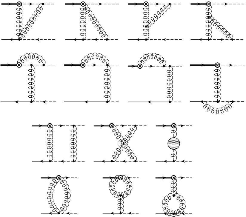
Figure 6: $\mbox{SCET}_{\rm I}$ graphs contributing to the matching of the currents $J_{j}^{B^{\prime}}$ (crossed circle) onto the $\mbox{SCET}_{\rm II}$ four-quark operators $O_{i}$. Full lines denote soft fields, dashed lines hard-collinear fields. Diagrams with soft gluons or scaleless loops are not shown.

In order to study the effect of next-to-leading order matching corrections, we now calculate the one-loop matching corrections to the jet functions ${\cal J}_{\parallel}$ and ${\cal J}_{\perp}$. The relevant diagrams are depicted in Figure 6. Contributions involving soft gluons cancel in the matching once the corresponding SCET_II diagrams are evaluated, so that only hard-collinear SCET_I diagrams need be considered. The $1/\epsilon$ poles are canceled by the renormalization constants of the SCET_I and SCET_II operators. Details of this calculation are presented in [32]. The results take the form

$${\cal J}_{\parallel}(u,v,L,\mu_{i}) = {4\pi C_{F}\alpha_{s}(\mu_{i})\over N}\,{1\over 2E\bar{u}}\left[-\delta(u-v)+\frac{\alpha_{s}(\mu_{i})}{4\pi}\,j_{\parallel}(u,v,L)+{\cal O}(\alpha_{s}^{2})\right],$$

$${\cal J}_{\perp}(u,v,L,\mu_{i}) = {4\pi C_{F}\alpha_{s}(\mu_{i})\over N}\,{1\over 2E\bar{u}}\left[-\delta(u-v)+\frac{\alpha_{s}(\mu_{i})}{4\pi}\,j_{\perp}(u,v,L)+{\cal O}(\alpha_{s}^{2})\right],$$ (117)

where $L=\ln(2E\omega/\mu_{i}^{2})$, and the functions $j_{\parallel}$ and $j_{\perp}$ are given by

$$j_{\parallel}(u,v,L) = j_{1}(u,v,L)+j_{2}(u,v,L)+j_{3}(u,v)\,,$$

$$j_{\perp}(u,v,L) = j_{1}(u,v,L)-j_{3}(u,v)\,,$$ (118)

with

$$j_{1}(u,v,L) = \delta(u-v)\,\Bigg{\{}T_{F}\,n_{f}\left[{20\over 9}-{4\over 3}\,(L+\ln\bar{u})\right]$$

$$\qquad\mbox{}+\left(C_{F}-{C_{A}\over 2}\right)\left[-(L+\ln u)^{2}-3(L+\ln\bar{u})+8-{\pi^{2}\over 2}\right]$$

$$\qquad\mbox{}-{C_{A}\over 2}\left[(L+\ln\bar{u})^{2}-{13\over 3}\,(L+\ln\bar{u})+{80\over 9}-{\pi^{2}\over 6}\right]\Bigg{\}}$$

$$\mbox{}+\left(C_{F}-{C_{A}\over 2}\right)\Bigg{\{}-2\left[{\theta(v-u)\over v-u}\,(L+\ln(v-u))+{\theta(u-v)\over u-v}\,(L+\ln(u-v))\right]_{+}$$

$$\qquad\mbox{}+\theta(1-u-v)\left[{2v\over\bar{u}\bar{v}}\left(L+\ln{v(1-u-v)\over\bar{u}}\right)+{2(1-u-v)\over u\bar{u}\bar{v}}\right]$$

$$\qquad\mbox{}+\theta(v-u)\left[{2\over\bar{u}}\,(L+\ln(v-u))+{2\over v-u}\,{\bar{v}\over\bar{u}}\,\ln{\bar{u}\over\bar{v}}-{2\over u\bar{u}}\right]$$

$$\qquad\mbox{}+\theta(u-v)\left[{2\over u\bar{v}}\,(L+\ln(u-v))+{2\over u-v}\,{v\bar{u}\over u\bar{v}}\,\ln{u\over v}-{2\over u\bar{v}}\right]\Bigg{\}}$$

$$\mbox{}+C_{F}\left\{{v(1+u)\over u\bar{v}}-\theta(v-u)\left[{2\over\bar{u}}\left(L+\ln{(v-u)\bar{v}\over\bar{u}}\right)+{(v-u)(1+u)\over u\bar{u}\bar{v}}\right]\right\},$$

$$j_{2}(u,v,L) = 2\left(C_{F}-{C_{A}\over 2}\right)\Bigg{\{}{1\over u}-\theta(u-v)\,{\bar{u}\over u\bar{v}}\left(L+\ln{(u-v)v\over u}\right)$$

$$\qquad\mbox{}-\theta(v-u)\,{\bar{v}\over u\bar{u}}\left(L+\ln{(v-u)\bar{v}\over\bar{u}}\right)$$

$$\qquad\mbox{}+\theta(1-u-v)\left[{(1-u-v)^{2}-uv\over u\bar{u}\bar{v}}\left(L+\ln{v(1-u-v)\over\bar{u}}\right)-{1\over u}\right]\Bigg{\}}$$

$$\mbox{}+2C_{F}\left[{v\bar{u}\over u}\,(L+\ln v\bar{v})-v-\theta(v-u)\,{(v-u)\over u\bar{u}}\left(L+\ln{(v-u)\bar{v}\over\bar{u}}\right)\right],$$

$$j_{3}(u,v) = C_{F}\left[-\frac{\bar{u}v}{u\bar{v}}\,\theta(u-v)-\theta(v-u)\right].$$ (119)

The plus distribution is defined as in (48). At one-loop order there are also matching coefficients onto evanescent operators. We adopt a renormalization scheme in which the matrix elements of these operators between physical states vanish [29], and so do not list their matching coefficients here. However, the choice of evanescent operators is not unique, and the jet functions as well as the matrix elements of the physical SCET_II four-quark operators depend on this choice. We have chosen the evanescent operators such that the matrix elements of the physical operators are given by the $\overline{\rm MS}$ LCDAs of the $B$ meson and light meson [32].

While the numerical impact of the one-loop matching corrections to the jet functions will be studied later, it is interesting at this point to use the explicit expressions in (6.2) to learn something about the “natural scale” to be used in the perturbative expansions for the jet functions. In the BLM scale-setting prescription, the scale in the coupling constant of the leading-order terms is chosen so as to absorb all terms proportional to $\beta_{0}=\frac{11}{3}\,C_{A}-\frac{4}{3}\,T_{F}n_{f}$ in the next-to-leading order corrections [33]. In the present case, this means that (for fixed $u$ and $\omega$ values) we should replace $\alpha_{s}(\mu_{i})\to\alpha_{s}(\mu_{\rm BLM})$, where

$$\mu_{\rm BLM}^{2}=e^{-\frac{5}{3}}\cdot 2\bar{u}E\omega$$ (120)

for both jet functions, which agrees with previous results reported in [34]. When applied to a specific process, such as the hard-scattering contributions to heavy-to-light form factors to be considered in Section 7, the BLM scale setting should be done after the convolution integrals over the LCDAs have been performed, which is equivalent to using mean values $\bar{u}\to e^{\langle\ln\bar{u}\rangle}$ and $\omega\to e^{\langle\ln\omega\rangle}$, weighted by the corresponding tree-level amplitudes, to define an effective scale for each decay process. The resulting BLM scales, while parametrically of order $\mu_{i}$, are numerically rather low, typically $\mu_{\rm BLM}\approx 0.7$ GeV or less. The smallness of these scales appears to suggest a poor convergence of the perturbative expansions of the jet functions. However, it turns out that the BLM prescription cannot be trusted in the present case. In the limit where we neglect the mild $y$-dependence of the coefficients $C_{j}^{B^{\prime}}(E,y,\mu_{i})$, it follows from (112) and (6.2) that the convolution integrals relevant to the hard-scattering contributions governed by the longitudinal jet function ${\cal J}_{\parallel}$ yield

$$\int_{0}^{\infty}\!{d\omega\over\omega}\,\phi_{B}(\omega,\mu_{i})\int_{0}^{1}\!\frac{du}{\bar{u}}\,\phi_{M}(u,\mu_{i})\,\alpha_{s}(\mu_{i})\left[1-\frac{\alpha_{s}(\mu_{i})}{4\pi}\int_{0}^{1}\!dy\,j_{\parallel}(u,y,\ln(2E\omega/\mu_{i}^{2}))\right]\quad$$

$$\propto\alpha_{s}(\mu_{i})\left\{1+{\alpha_{s}(\mu_{i})\over 4\pi}\left[{4\over 3}\left\langle\ln^{2}{2E\omega\over\mu_{i}^{2}}\right\rangle+\left(-{19\over 3}+{\pi^{2}\over 9}\right)\left\langle\ln{2E\omega\over\mu_{i}^{2}}\right\rangle+3.99\right]\right\},$$ (121)

where $\langle\dots\rangle$ denotes an average over the $B$-meson LCDA $\phi_{B}(\omega,\mu_{i})$ with measure $d\omega/\omega$, and for simplicity we have assumed the asymptotic form $\phi_{M}(u,\mu_{i})=6u\bar{u}$ for the LCDA of the light meson. The corresponding result for the jet function ${\cal J}_{\perp}$ is obtained by replacing $j_{\parallel}\to j_{\perp}$, in which case the coefficient of the single logarithm changes to $(-6+\frac{\pi^{2}}{9})$, and the constant term changes to 0.73. If scale $\mu_{i}$ is chosen such that the logarithms appearing in this expression are not too large, then (at least through one-loop order) the perturbative corrections are of moderate size. For comparison, keeping only the BLM terms of order $\beta_{0}\alpha_{s}^{2}$, we would obtain

$$\alpha_{s}(\mu_{i})\left\{1+{\alpha_{s}(\mu_{i})\over 4\pi}\left[-{25\over 3}\left\langle\ln{2E\omega\over\mu_{i}^{2}}\right\rangle+26.39\right]\right\}$$ (122)

instead of the expression in the second line of (6.2). We conclude that the BLM prescription overestimates the size of the ${\cal O}(\alpha_{s}^{2})$ corrections by large amounts. The perturbative expansions of the jet functions at a scale $\mu_{i}=\sqrt{2E\Lambda_{h}}\approx 1.5$ GeV appear to be reasonably well behaved.

6.3 Sudakov resummation in SCET_II

Having performed the matching onto SCET_II, we now wish to evolve the momentum-space coefficient functions $D_{i}$ in (111) from the intermediate scale $\mu_{i}\sim\sqrt{2E\Lambda_{\rm QCD}}$ down to a hadronic scale $\mu$, which is independent of the large energy $E$. This can be achieved by solving the integro-differential RG equation [15]

$${d\over d\ln\mu}\,D_{i}(E,\omega^{\prime},u^{\prime},\mu)=\int_{0}^{\infty}\!d\omega\int_{0}^{1}\!du\,\gamma_{\Gamma}(\omega,\omega^{\prime},u,u^{\prime},\mu)\,D_{i}(E,\omega,u,\mu)\,.$$ (123)

The anomalous dimension $\gamma_{\Gamma}$ depends on the spin-parity quantum numbers of the light final-state meson $M$. As before, we must distinguish two cases: $\Gamma=\,\parallel$ for $M=P,V_{\parallel}$, and $\Gamma=\,\perp$ for $M=V_{\perp}$. The anomalous dimension may be decomposed as

$$\gamma_{\Gamma}(\omega,\omega^{\prime},u,u^{\prime},\mu)=\delta(\omega-\omega^{\prime})\,K_{\Gamma}(u,u^{\prime})+\delta(u-u^{\prime})\,H(\omega,\omega^{\prime},\mu)\,,$$ (124)

where

$$v\bar{v}\,K_{\Gamma}(u,v) = {C_{F}\alpha_{s}\over\pi}\,\Bigg{\{}-\left[u\bar{v}\,{\theta(v-u)\over v-u}+v\bar{u}\,{\theta(u-v)\over u-v}\right]_{+}+{1\over 2}\,u\bar{u}\,\delta(u-v)$$ (125)

$$\qquad\mbox{}-c_{\Gamma}\Big{[}u\bar{v}\,\theta(v-u)+v\bar{u}\,\theta(u-v)\Big{]}\Bigg{\}}+{\cal O}(\alpha_{s}^{2})\,,$$

with $c_{\parallel}=1$, $c_{\perp}=0$ is the Brodsky-Lepage kernel [24], and

$$H(\omega,\omega^{\prime},\mu) = \left[\Gamma_{\rm cusp}(\alpha_{s})\,\ln{\mu\over\omega}+\gamma(\alpha_{s})\right]\delta(\omega-\omega^{\prime})+\omega\,\Gamma(\omega,\omega^{\prime},\alpha_{s})$$

$$= {C_{F}\alpha_{s}\over\pi}\,\Bigg{\{}\left(\ln{\mu\over\omega}-{5\over 4}\right)\delta(\omega-\omega^{\prime})-\omega\left[{\theta(\omega-\omega^{\prime})\over\omega(\omega-\omega^{\prime})}+{\theta(\omega^{\prime}-\omega)\over\omega^{\prime}(\omega^{\prime}-\omega)}\right]_{+}\Bigg{\}}+{\cal O}(\alpha_{s}^{2})$$

is the corresponding kernel governing the evolution of the $B$-meson LCDA [20, 36].

As a consequence of the conformal symmetry of QCD at the classical level, the kernel $v\bar{v}\,K_{\Gamma}(u,v)$ is symmetric in $u$ and $v$, and $K_{\Gamma}$ is diagonalized by Gegenbauer polynomials (cf. (96) in Section 5.3). We write

$$\int_{0}^{1}\!du\,K_{\Gamma}(u,v)\,\varphi_{n}(u)=\kappa_{\Gamma,n}\,\varphi_{n}(v)\,,$$ (127)

where at one-loop order

$$\kappa_{\Gamma,n}={C_{F}\alpha_{s}\over\pi}\left[2(H_{n+1}-1)+{1\over 2}-{c_{\Gamma}\over(n+1)(n+2)}\right].$$ (128)

We choose the normalization of $\varphi_{n}$ such that they are orthonormal in the measure $u\bar{u}\,du$ on the unit interval,

$$\varphi_{n}(u)=2\sqrt{2n+3\over(n+1)(n+2)}\,C_{n}^{(3/2)}(2u-1)=\sqrt{(2n+3)(n+2)\over n+1}\,P_{n}^{(1,1)}(2u-1)\,.$$ (129)

After expanding the coefficients $D_{i}(E,\omega,u,\mu)$ on the basis of eigenfunctions $\varphi_{n}(u)$, the RG equation for each Gegenbauer moment is solved as in [20]. The result reads

$$D_{i}(E,\omega,u,\mu) = \frac{1}{2E\omega}\left({\omega\over\mu}\right)^{-a(\mu_{i},\mu)}e^{S(\mu,\mu_{i})}\,\sum_{n=0}^{\infty}\varphi_{n}(u)$$

$$\times \int_{0}^{1}\!dy\,C^{B^{\prime}}_{j}(E,y,\mu_{i})\int_{0}^{1}\!dx\,x\bar{x}\,\varphi_{n}(x)\,{\cal J}^{\prime}_{ij}(x,y,\nabla_{\eta},\mu_{i})\,\bigg{(}{2E\omega\over\mu_{i}^{2}}\bigg{)}^{\eta}\,e^{V_{\Gamma,n}(\mu_{i},\mu,\eta)}\bigg{|}_{\eta=0},$$

where $S(\mu,\mu_{i})$ and $a(\mu_{i},\mu)$ are given in (64) and (65), the jet functions ${\cal J}^{\prime}_{ij}$ in the primed basis are obtained from (112) by replacing $2E\omega/\mu_{i}^{2}\to\nabla_{\eta}$, and

$$V_{\Gamma,n}(\mu_{i},\mu,\eta)=\int_{\alpha_{s}(\mu_{i})}^{\alpha_{s}(\mu)}{d\alpha\over\beta(\alpha)}\,\bigg{[}{\cal F}(\eta-a(\mu_{i},\mu(\alpha)),\alpha)+\kappa_{\Gamma,n}(\alpha)+\gamma(\alpha)\bigg{]}\,,$$ (131)

with

$${\cal F}(\eta,\alpha_{s}) \equiv \int_{0}^{\infty}\!d\omega\,\omega^{\prime}\,\Gamma(\omega,\omega^{\prime},\alpha_{s})\left({\omega\over\omega^{\prime}}\right)^{\eta}$$ (132)

$$= \Gamma_{\rm cusp}^{\rm 1-loop}(\alpha_{s})\,\Big{[}\psi(1+\eta)+\psi(1-\eta)+2\gamma_{E}\Big{]}+{\cal O}(\alpha_{s}^{2})\,.$$

For a complete leading-order solution, we require the two-loop expression for $\Gamma_{\rm cusp}$ appearing in $S(\mu,\mu_{i})$, one-loop expressions for the remaining anomalous dimensions in $a(\mu_{i},\mu)$ and $V_{\Gamma,n}(\mu_{i},\mu,\eta)$, and tree-level matching conditions for the jet functions. At this order, the relevant expansions are

$$S(\mu,\mu_{i}) = \frac{\Gamma_{0}}{4\beta_{0}^{2}}\left[\frac{4\pi}{\alpha_{s}(\mu)}\left(1-{r_{2}}+\ln r_{2}\right)+\frac{\beta_{1}}{2\beta_{0}}\,\ln^{2}r_{2}-\left(\frac{\Gamma_{1}}{\Gamma_{0}}-\frac{\beta_{1}}{\beta_{0}}\right)\left({1\over r_{2}}-1+\ln r_{2}\right)\right],$$

$$a(\mu_{i},\mu) = -\frac{\Gamma_{0}}{2\beta_{0}}\,\ln r_{2}\,,$$

$$V_{\Gamma,n}(\mu_{i},\mu,0) = \ln{\Gamma\Big{(}1-{\Gamma_{0}\over 2\beta_{0}}\,\ln{r_{2}}\Big{)}\over\Gamma\Big{(}1+{\Gamma_{0}\over 2\beta_{0}}\,\ln{r_{2}}\Big{)}}-\gamma_{E}\,{\Gamma_{0}\over\beta_{0}}\,\ln{r_{2}}-{1\over 2\beta_{0}}\left(\kappa_{\Gamma,n}^{(0)}+\gamma_{0}\right)\ln{r_{2}}\,,$$ (133)

where $r_{2}=\alpha_{s}(\mu)/\alpha_{s}(\mu_{i})\geq 1$, and as usual we have expanded

$$\kappa_{\Gamma,m}=\kappa_{\Gamma,m}^{(0)}\,{\alpha_{s}\over 4\pi}+\dots\,,\qquad\gamma=\gamma_{0}\,{\alpha_{s}\over 4\pi}+\dots\,.$$ (134)

7 Application to heavy-to-light form factors

In this section we apply our results to obtain resummed expressions for the hard-scattering contributions to heavy-to-light form factors at large recoil energy. We begin by recalling the definitions of the ten form factors describing $B$ decays into pseudoscalar and vector mesons. Equating these definitions to the corresponding effective-theory expressions shows that at leading order in $1/E$ only eight of the form factors are independent. As shown in (1), in this approximation the form factors are given by the sum of a soft-overlap contribution, expressed in terms of universal non-perturbative matrix elements $\zeta_{M}(E)$ (where $M=P$, $V_{\parallel}$, $V_{\perp}$ depending on the spin-parity quantum numbers of the light final-state meson), and a hard-scattering contribution, given by a convolution integral over meson LCDAs. We focus on the second term and present general, resummed expressions for the corresponding hard-scattering kernels. The results are particularly simple when hard matching corrections are ignored. In this case, for a given final-state meson $M$, the hard-scattering contributions to all $B\to M$ form factors can be parameterized in terms of a universal quantity $H_{M}$. The Sudakov suppression factors are mild in all cases. In order to investigate the relative importance of running and matching corrections, we apply our previous one-loop matching results for the scalar current to obtain the one-loop corrected hard-scattering contribution to the vector-current form factor $F_{0}$, and to the form factor $F_{+}$ at maximum recoil ($q^{2}=0$).

7.1 Form-factor definitions and factorization formulae

We begin by recalling the definitions of the form factors parameterizing $B$ decays into pseudoscalar ($P$) and vector ($V$) mesons, following the conventions of [13] (we use the sign convention $\epsilon^{0123}=-1$):

$$\langle P(p^{\prime})|\bar{q}\,\gamma^{\mu}b|\bar{B}(p)\rangle = F_{+}(q^{2})\left(p^{\mu}+p^{\prime\mu}-{m_{B}^{2}-m_{P}^{2}\over q^{2}}\,q^{\mu}\right)+F_{0}(q^{2})\,{m_{B}^{2}-m_{P}^{2}\over q^{2}}\,q^{\mu}\,,$$

$$\langle P(p^{\prime})|\bar{q}\,\sigma^{\mu\nu}q_{\nu}\,b|\bar{B}(p)\rangle = {iF_{T}(q^{2})\over m_{B}+m_{P}}\left[q^{2}\,(p^{\mu}+p^{\prime\mu})-(m_{B}^{2}-m_{P}^{2})\,q^{\mu}\right],$$

$$\langle V(p^{\prime},\eta)|\bar{q}\,\gamma^{\mu}b|\bar{B}(p)\rangle = {2iV(q^{2})\over m_{B}+m_{V}}\,{\epsilon}^{\mu\nu\rho\sigma}\eta^{*}_{\nu}\,p^{\prime}_{\rho}\,p_{\sigma}\,,$$

$$\langle V(p^{\prime},\eta)|\bar{q}\,\gamma^{\mu}\gamma_{5}\,b|\bar{B}(p)\rangle = 2m_{V}A_{0}(q^{2})\,{\eta^{*}\cdot q\over q^{2}}\,q^{\mu}+(m_{B}+m_{V})\,A_{1}(q^{2})\left(\eta^{*\mu}-{\eta^{*}\cdot q\over q^{2}}\,q^{\mu}\right)$$

$$\mbox{}-A_{2}(q^{2})\,{\eta^{*}\cdot q\over m_{B}+m_{V}}\left(p^{\mu}+p^{\prime\mu}-{m_{B}^{2}-m_{V}^{2}\over q^{2}}\,q^{\mu}\right),$$

$$\langle V(p^{\prime},\eta)|\bar{q}\,\sigma^{\mu\nu}q_{\nu}\,b|\bar{B}(p)\rangle = -2T_{1}(q^{2})\,{\epsilon}^{\mu\nu\rho\sigma}\eta^{*}_{\nu}\,p^{\prime}_{\rho}\,p_{\sigma}\,,$$

$$\langle V(p^{\prime},\eta)|\bar{q}\,\sigma^{\mu\nu}\gamma_{5}\,q_{\nu}\,b|\bar{B}(p)\rangle = -i\,T_{2}(q^{2})\left[(m_{B}^{2}-m_{V}^{2})\,\eta^{*\mu}-\eta^{*}\cdot q\,(p^{\mu}+p^{\prime\mu})\right]$$ (135)

$$\mbox{}-i\,T_{3}(q^{2})\,\eta^{*}\cdot q\left[q^{\mu}-{q^{2}\over m_{B}^{2}-m_{V}^{2}}\,(p^{\mu}+p^{\prime\mu})\right].$$

Here $q=p-p^{\prime}$ is the momentum transfer, and $\eta$ denotes the polarization vector of the vector meson, which satisfies $\eta\cdot p^{\prime}=0$ and $\eta\cdot\eta^{*}=-1$. The polarization vector for longitudinally polarized vector mesons is given by

$$\eta_{\parallel}^{\mu}={p^{\prime\,\mu}\over m_{V}}-{m_{V}\over\bar{n}\cdot p^{\prime}}\,\bar{n}^{\mu}\simeq{E\over m_{V}}\,\frac{n^{\mu}}{n\cdot v}\,.$$ (136)

For the evaluation of the hadronic matrix elements entering the hard-scattering contributions to the form factors, we need the definitions of the leading-twist LCDAs for the light mesons in terms of SCET_II fields. They are [9]

$$\langle P(p^{\prime})|\bar{{\mathcal{X}}}_{c}(s\bar{n})\,\Gamma\,{\hbox to0.0pt{\hskip 0.56917pt/\hss}{\bar{n}}\over 2}\,{\mathcal{X}}_{c}(0)|0\rangle = {if_{P}\over 4}\,\bar{n}\cdot p^{\prime}\,\,{\rm tr}\left(\gamma_{5}\,\Gamma\,{\hbox to0.0pt{\hskip 0.56917pt/\hss}{\bar{n}}\hbox to0.0pt{\hskip 0.56917pt/\hss}{n}\over 4}\right)\int_{0}^{1}\!du\,e^{ius\bar{n}\cdot p^{\prime}}\,\phi_{P}(u,\mu)\,,$$

$$\langle V_{\parallel}(p^{\prime})|\bar{{\mathcal{X}}}_{c}(s\bar{n})\,\Gamma\,{\hbox to0.0pt{\hskip 0.56917pt/\hss}{\bar{n}}\over 2}\,{\mathcal{X}}_{c}(0)|0\rangle = -{if_{V_{\parallel}}\over 4}\,\bar{n}\cdot p^{\prime}\,\,{\rm tr}\left(\Gamma\,{\hbox to0.0pt{\hskip 0.56917pt/\hss}{\bar{n}}\hbox to0.0pt{\hskip 0.56917pt/\hss}{n}\over 4}\right)\int_{0}^{1}\!du\,e^{ius\bar{n}\cdot p^{\prime}}\,\phi_{V_{\parallel}}(u,\mu)\,,$$

$$\langle V_{\perp}(p^{\prime},\eta)|\bar{{\mathcal{X}}}_{c}(s\bar{n})\,\Gamma\,{\hbox to0.0pt{\hskip 0.56917pt/\hss}{\bar{n}}\over 2}\,{\mathcal{X}}_{c}(0)|0\rangle = {if_{V_{\perp}}(\mu)\over 4}\,\bar{n}\cdot p^{\prime}\,\,{\rm tr}\left(\hbox to0.0pt{\hskip 0.56917pt/\hss}{\eta^{*}_{\perp}}\,\Gamma\,{\hbox to0.0pt{\hskip 0.56917pt/\hss}{\bar{n}}\hbox to0.0pt{\hskip 0.56917pt/\hss}{n}\over 4}\right)\int_{0}^{1}\!du\,e^{ius\bar{n}\cdot p^{\prime}}\,\phi_{V_{\perp}}(u,\mu)\,,\qquad$$ (137)

where the $\phi_{M}$ are normalized according to $\int_{0}^{1}\!du\,\phi_{M}(u,\mu)=1$. Note that the transverse vector-meson decay constants are scale dependent. Below, we will sometimes write $f_{M}(\mu)$ as a generic notation for the light-meson decay constants, keeping in mind that a scale dependence is present only in the case of $f_{V_{\perp}}$. The LCDA for the $B$-meson is defined as [35, 36]

$$\langle 0|\bar{{\mathcal{Q}}}_{s}(tn)\,{\hbox to0.0pt{\hskip 0.56917pt/\hss}{n}\over 2}\,\Gamma\,{\mathcal{H}}(0)|\bar{B}_{v}\rangle=-{i\sqrt{m_{B}}\,F(\mu)\over 2}\,\,{\rm tr}\left({\hbox to0.0pt{\hskip 0.56917pt/\hss}{n}\over 2}\,\Gamma\,{1+\hbox to0.0pt{\hskip 0.56917pt/\hss}{v}\over 2}\,\gamma_{5}\right)\int_{0}^{\infty}\!d\omega\,e^{-i\omega tn\cdot v}\,\phi_{B}(\omega,\mu)\,,$$ (138)

where $\bar{B}_{v}$ denotes the $B$-meson state defined in HQET, and $F$ is related to the asymptotic value of the $B$-meson decay constant in the heavy-quark limit (see below).

For completeness, we list also the soft-overlap contributions to form factors, parameterized in terms of universal matrix elements $\zeta_{M}$ [12, 13]. At leading order in $1/E$, we define

$$\langle P(p^{\prime})|\bar{{\mathcal{X}}}_{hc}\,\Gamma\,h|\bar{B}_{v}\rangle = 2E\,\zeta_{P}(E)\,\,{\rm tr}\left({\hbox to0.0pt{\hskip 0.56917pt/\hss}{\bar{n}}\hbox to0.0pt{\hskip 0.56917pt/\hss}{n}\over 4}\,\Gamma\,{1+\hbox to0.0pt{\hskip 0.56917pt/\hss}{v}\over 2}\right),$$

$$\langle V_{\parallel}(p^{\prime})|\bar{{\mathcal{X}}}_{hc}\,\Gamma\,h|\bar{B}_{v}\rangle = -2E\,\zeta_{V_{\parallel}}(E)\,\,{\rm tr}\left({\hbox to0.0pt{\hskip 0.56917pt/\hss}{\bar{n}}\hbox to0.0pt{\hskip 0.56917pt/\hss}{n}\over 4}\,\Gamma\,{1+\hbox to0.0pt{\hskip 0.56917pt/\hss}{v}\over 2}\,\gamma_{5}\right),$$

$$\langle V_{\perp}(p^{\prime})|\bar{{\mathcal{X}}}_{hc}\,\Gamma\,h|\bar{B}_{v}\rangle = 2E\,\zeta_{V_{\perp}}(E)\,\,{\rm tr}\left(\hbox to0.0pt{\hskip 0.56917pt/\hss}{\eta}^{*}_{\perp}\,{\hbox to0.0pt{\hskip 0.56917pt/\hss}{\bar{n}}\hbox to0.0pt{\hskip 0.56917pt/\hss}{n}\over 4}\,\Gamma\,{1+\hbox to0.0pt{\hskip 0.56917pt/\hss}{v}\over 2}\,\gamma_{5}\right).$$ (139)

The definitions are given in terms of SCET_I currents. As shown in [8], the functions $\zeta_{M}(E)$ can be decomposed further into matrix elements of SCET_II operators. These operators all satisfy the same symmetry relations, and the linear combinations contributing to the form factor behave under renormalization in precisely the same way as the SCET_I operators used in the definitions (7.1).

To simplify the factorization formulae, it proves convenient to write the coefficient functions in the form

$$D_{i}(E,\omega,u,\mu)\equiv{1\over\omega}\,{4K_{F}(\mu)\over m_{B}f_{B}}\,T_{i}(E,\omega,u,\mu)\,,$$ (140)

which serves as a definition of the hard-scattering kernels $T_{i}$. Here $K_{F}$ relates the HQET parameter $F$ in (138) to the physical $B$-meson decay constant, $f_{B}\sqrt{m_{B}}=K_{F}(\mu)\,F(\mu)$, up to corrections of order $\Lambda_{\rm QCD}/m_{b}$. At next-to-leading order

$$K_{F}(\mu)=1+{C_{F}\alpha_{s}(\mu)\over 4\pi}\left(3\ln{m_{b}\over\mu}-2\right).$$ (141)

With all of the definitions in place, it is now a straightforward matter to equate QCD matrix elements to the corresponding SCET expressions. For the scalar and pseudoscalar currents, for example, we obtain

$${1\over m_{B}}\,\langle P(p^{\prime})|\bar{q}\,b|\bar{B}(p)\rangle = {2E\over m_{B}}\,C^{A}_{S}(E,\mu)\,\zeta_{P}(E,\mu)$$

$$+ {2E\over m_{B}}\int_{0}^{\infty}\!{d\omega\over\omega}\,\phi_{B}(\omega,\mu)\int_{0}^{1}\!du\,f_{P}\,\phi_{P}(u,\mu)\,T_{S}(E,\omega,u,\mu)$$

$$\equiv {2E\over m_{B}}\left[C^{A}_{S}\,\zeta_{P}+\phi_{B}\otimes f_{P}\,\phi_{P}\otimes T_{S}\right],$$

$${1\over m_{B}}\,\langle V_{\parallel}(p^{\prime})|\bar{q}\,\gamma_{5}\,b|\bar{B}(p)\rangle = -{2E\over m_{B}}\left[C^{A}_{S}\,\zeta_{V_{\parallel}}+\phi_{B}\otimes f_{V_{\parallel}}\,\phi_{V_{\parallel}}\otimes T_{S}\right],$$ (142)

where in the second line we have introduced a symbolic notation for the convolution integrals. In general, the scale $\mu$ in the soft-overlap terms could be taken different from that in the hard-scattering terms. Similarly, from the matrix elements of vector and tensor currents we find the relations

$$F_{+} = \left(C^{A}_{V1}+{E\over m_{B}}\,C^{A}_{V2}+C^{A}_{V3}\right)\zeta_{P}+\phi_{B}\otimes f_{P}\,\phi_{P}\otimes\left(T_{V1}+{E\over m_{B}}\,T_{V2}\right),$$

$$\frac{m_{B}}{2E}\,F_{0} = \left[C^{A}_{V1}+\!\left(1-{E\over m_{B}}\right)\!C^{A}_{V2}+C^{A}_{V3}\right]\zeta_{P}+\phi_{B}\otimes f_{P}\,\phi_{P}\otimes\!\left[T_{V1}+\!\left(1-{E\over m_{B}}\right)\!T_{V2}\right]\!,$$

$$\frac{m_{B}}{m_{B}+m_{P}}\,F_{T} = \left(C_{T1}^{A}-\frac{1}{2}\,C_{T2}^{A}+\frac{1}{2}\,C_{T4}^{A}\right)\zeta_{P}+\phi_{B}\otimes f_{P}\,\phi_{P}\otimes\frac{1}{2}\,T_{T1}\,,$$

$$A_{0} = \!\left[C^{A}_{V1}+\!\left(\!1-{E\over m_{B}}\right)\!C^{A}_{V2}+C^{A}_{V3}\right]\!\zeta_{V_{\parallel}}+\phi_{B}\otimes f_{V_{\parallel}}\,\phi_{V_{\parallel}}\otimes\!\left[T_{V1}+\!\left(\!1-{E\over m_{B}}\right)\!T_{V2}\right]\!,$$

$$\frac{m_{B}+m_{V}}{2E}\,A_{1} = C^{A}_{V1}\,\zeta_{V_{\perp}}+\phi_{B}\otimes f_{V_{\perp}}\,\phi_{V_{\perp}}\otimes T_{V3}\,,$$

$$\frac{m_{B}}{m_{B}+m_{V}}\,V = C^{A}_{V1}\,\zeta_{V_{\perp}}+\phi_{B}\otimes f_{V_{\perp}}\,\phi_{V_{\perp}}\otimes T_{V3}\,,$$

$$\frac{Em_{B}\,(V-A_{2})}{m_{V}(m_{B}\!+\!m_{V})} = \left(C^{A}_{V1}+{E\over m_{B}}\,C^{A}_{V2}+C^{A}_{V3}\right)\zeta_{V_{\parallel}}+\phi_{B}\otimes f_{V_{\parallel}}\,\phi_{V_{\parallel}}\otimes\left(T_{V1}+{E\over m_{B}}\,T_{V2}\right),$$

$$T_{1} = \left[C^{A}_{T1}-{1\over 2}\left(1-{E\over m_{B}}\right)C^{A}_{T2}-{1\over 2}\,C^{A}_{T3}\right]\zeta_{V_{\perp}}$$

$$\mbox{}-\frac{1}{2}\,\phi_{B}\otimes f_{V_{\perp}}\,\phi_{V_{\perp}}\otimes\left[T_{T2}+\left(1-{E\over m_{B}}\right)T_{T3}\right],$$

$$\frac{m_{B}}{2E}\,T_{2} = \left[C^{A}_{T1}-{1\over 2}\left(1-{E\over m_{B}}\right)C^{A}_{T2}-{1\over 2}\,C^{A}_{T3}\right]\zeta_{V_{\perp}}$$

$$\mbox{}-\frac{1}{2}\,\phi_{B}\otimes f_{V_{\perp}}\,\phi_{V_{\perp}}\otimes\left[T_{T2}+\left(1-{E\over m_{B}}\right)T_{T3}\right],$$

$$\frac{m_{B}T_{2}-2E\,T_{3}}{2m_{V}}\! = \!\left(C^{A}_{T1}-{1\over 2}\,C^{A}_{T2}+{1\over 2}\,C^{A}_{T4}\right)\zeta_{V_{\parallel}}+\phi_{B}\otimes f_{V_{\parallel}}\,\phi_{V_{\parallel}}\otimes\frac{1}{2}\,T_{T1}\,.$$ (143)

We have dropped terms of relative order $(m_{M}/E)^{2}$, where $m_{M}$ is the light meson mass. Recall that we have defined $E\equiv v\cdot P_{-}$, which differs from the true energy by an amount of order $m_{M}^{2}/E$. Also, at leading order in $\Lambda_{\rm QCD}/m_{b}$ there is no difference between $m_{B}$ and $m_{b}$. The results for $F_{+}$, $F_{0}$ and $F_{T}$ in (7.1) agree at tree level with the corresponding expressions in [19]. Beyond tree level, and to any order in perturbation theory, we find that there is still only a single jet function for decays into a given light final-state meson, e.g. ${\cal J}_{\parallel}$ for a pseudoscalar meson. This implies that the two functions $J_{a}$ and $J_{b}$ introduced in [19] are not independent. Our result has important implications for the universality of hard-scattering corrections, which we discuss in more detail in the following subsection. The general results (7.1) establish that the form-factor relations

$$A_{1}(q^{2})={2Em_{B}\over(m_{B}+m_{V})^{2}}\,V(q^{2})\,,\qquad T_{2}(q^{2})={2E\over m_{B}}\,T_{1}(q^{2})\,,$$ (144)

are rigorous predictions of QCD at leading order in $1/E$, and to all orders in $\alpha_{s}$. These relations were conjectured in [39], and they were shown to hold at one-loop order in [13].

The scalar and pseudoscalar currents may be related to the vector and axial-vector currents using the equation of motion for the quark fields, as in (3.2). When applied to the matrix elements appearing in (7.1) and (7.1), it follows that (setting as previously the light quark masses to zero)

$$\frac{\overline{m}_{b}(\mu_{\rm QCD})}{m_{B}^{2}}\,\langle P(p^{\prime})|[\bar{q}\,b](\mu_{\rm QCD})|\bar{B}(p)\rangle = \left(1-{m_{P}^{2}\over m_{B}^{2}}\right)F_{0}(q^{2})=F_{0}(q^{2})+\dots\,,$$

$$\frac{\overline{m}_{b}(\mu_{\rm QCD})}{m_{B}^{2}}\,\langle V_{\parallel}(p^{\prime})|[\bar{q}\,\gamma_{5}\,b](\mu_{\rm QCD})|\bar{B}(p)\rangle = -{2m_{V}\,\eta^{*}_{\parallel}\cdot q\over m_{B}^{2}}\,A_{0}(q^{2})=-{2E\over m_{B}}\,A_{0}(q^{2})+\dots\,,\qquad$$ (145)

where the dots represent terms of order $m_{M}^{2}/m_{B}^{2}$. Comparison with (7.1) shows that to all orders in perturbation theory

$$C^{A}_{V1}+\left(1-{E\over m_{b}}\right)C^{A}_{V2}+C^{A}_{V3} = \frac{\overline{m}_{b}(\mu_{\rm QCD})}{m_{b}}\,C^{A}_{S}\,,$$

$$T_{V1}+\left(1-{E\over m_{b}}\right)T_{V2} = \frac{\overline{m}_{b}(\mu_{\rm QCD})}{m_{b}}\,T_{S}\,.$$ (146)

These are the SCET_II realizations of the SCET_I coefficient relations found in (3.2).

7.2 Sudakov resummation for the hard-scattering contributions

We now apply the results of Sections 5 and 6 to obtain completely general, resummed expressions for the hard-scattering kernels $T_{i}$ appearing in the form-factors (7.1). Starting from the defining relation (140) for $T_{i}$, and combining it with the result (6.3) for the coefficients $D_{i}$, we obtain

$$T_{i}(E,\omega,u,\mu) = {m_{B}f_{B}\over 8E}\,{e^{V_{F}(\mu_{h},\mu)}\over K_{F}(\mu_{h})}\left({2E\over\mu_{h}}\right)^{a(\mu_{h},\mu_{i})}\left({\omega\over\mu}\right)^{-a(\mu_{i},\mu)}e^{S(\mu_{h},\mu_{i})+S(\mu,\mu_{i})}$$ (147)

$$\times \sum_{n=0}^{\infty}\varphi_{n}(u)\int_{0}^{1}\!dy\int_{0}^{1}\!dv\,U_{\Gamma}(y,v,\mu_{h},\mu_{i})\,C_{j}^{B^{\prime}}(E,v,\mu_{h})$$

$$\times \int_{0}^{1}\!dx\,x\bar{x}\,\varphi_{n}(x)\,{\cal J}^{\prime}_{ij}(x,y,\nabla_{\eta},\mu_{i})\left({2E\omega\over\mu_{i}^{2}}\right)^{\eta}e^{V_{\Gamma,n}(\mu_{i},\mu,\eta)}\bigg{|}_{\eta=0}\,.$$

We have used (63) to express the coefficients $C_{j}^{B^{\prime}}(E,y,\mu_{i})$ at the intermediate scale, which enter in (6.3), in terms of their matching conditions at the high scale $\mu_{h}$. Also, we have rewritten $K_{F}(\mu)=e^{-V_{F}(\mu_{h},\mu)}\,K_{F}(\mu_{h})$, where

$$V_{F}(\mu_{h},\mu)=-\int_{\alpha_{s}(\mu_{h})}^{\alpha_{s}(\mu)}{d\alpha\over\beta(\alpha)}\,\gamma_{F}(\alpha)={\gamma_{F,0}\over 2\beta_{0}}\,\ln{r_{1}r_{2}}+\dots$$ (148)

is the solution to the evolution equation

$${d\over d\ln{\mu}}\,K_{F}=\gamma_{F}\,K_{F}\,,\qquad\gamma_{F}=\sum_{n=0}^{\infty}\gamma_{F,n}\left({\alpha_{s}\over 4\pi}\right)^{n+1},$$ (149)

with $\gamma_{F,0}=-3C_{F}$. As previously, $r_{1}=\alpha_{s}(\mu_{i})/\alpha_{s}(\mu_{h})$ and $r_{2}=\alpha_{s}(\mu)/\alpha_{s}(\mu_{i})$. In (147) all large logarithms are resummed into the various evolution functions. The matching coefficients $K_{F}(\mu_{h})$, $C_{j}^{B^{\prime}}(E,v,\mu_{h})$, and ${\cal J}^{\prime}_{ij}(x,y,\nabla_{\eta},\mu_{i})$ can be calculated reliably in fixed-order perturbation theory. The expressions for the kernels $T_{i}$ are formally (to the order we are working) independent of the two matching scales $\mu_{h}$ and $\mu_{i}$. A dependence on the low scale $\mu$ remains, which will cancel against the scale dependence of the hadronic matrix elements of the SCET_II operators.

The general result (147) simplifies considerably when hard matching corrections at the high scale $\mu_{h}\sim m_{b}$ are ignored. In this case $K_{F}(\mu_{h})=1$, and using the fact that the tree-level matching conditions for $C_{j}^{B^{\prime}}(E,v,\mu_{h})$ are independent of $v$, it follows that

$$\int_{0}^{1}\!dv\,U_{\Gamma}(y,v,\mu_{h},\mu_{i})\,C_{j}^{B^{\prime}}(E,v,\mu_{h})=U_{\Gamma}(y,\mu_{h},\mu_{i})\,C_{j}^{B^{\prime}}(E,\mu_{h})\,,$$ (150)

where $U_{\Gamma}(y,\mu_{h},\mu_{i})$ are the functions shown in Figure 4. Using the tree-level matching conditions compiled in (26)–(3.2) along with the relations (4) and (4), it is straightforward to evaluate the products ${\cal J}^{\prime}_{ij}\,C_{j}^{B^{\prime}}(E,\mu_{h})$ for the various kernels $T_{i}$, with the matrices ${\cal J}^{\prime}_{ij}$ as given in (115). We find

$$T_{S}:~{}-{\cal J}_{\parallel}\,,$$

$$T_{V1}:~{}\left(1-\frac{2E}{m_{b}}\right){\cal J}_{\parallel}\,,\qquad T_{V2}:~{}-2{\cal J}_{\parallel}\,,\qquad T_{V3}:~{}0\,,$$

$$T_{T1}:~{}2{\cal J}_{\parallel}\,,\qquad T_{T2}:~{}\frac{4E}{m_{b}}\,{\cal J}_{\perp}\,,\qquad T_{T3}:~{}0\,.$$ (151)

It follows that the convolution integrals for the hard-scattering contributions to the form factors in (7.1) may be written in terms of three universal functions

$$H_{M} \equiv -{Ef_{B}\over 2m_{B}}\,\left({2E\over\mu_{h}}\right)^{a(\mu_{h},\mu_{i})}e^{S(\mu_{h},\mu_{i})+S(\mu,\mu_{i})+V_{F}(\mu_{h},\mu)}\,\sum_{n=0}^{\infty}\int_{0}^{1}\!du\,\varphi_{n}(u)\,f_{M}(\mu)\,\phi_{M}(u,\mu)$$ (152)

$$\times \int_{0}^{\infty}\!{d\omega\over\omega}\,\phi_{B}(\omega,\mu)\left({\omega\over\mu}\right)^{-a(\mu_{i},\mu)}\!\int_{0}^{1}\!dy\,U_{\Gamma}(y,\mu_{h},\mu_{i})$$

$$\times \int_{0}^{1}\!dx\,x\bar{x}\,\varphi_{n}(x)\,{\cal J}_{\Gamma}(x,y,\nabla_{\eta},\mu_{i})\left({2E\omega\over\mu_{i}^{2}}\right)^{\eta}e^{V_{\Gamma,n}(\mu_{i},\mu,\eta)}\bigg{|}_{\eta=0}\,,$$

where $\Gamma=\,\parallel$ for $M=P$ or $V_{\parallel}$, and $\Gamma=\,\perp$ for $M=V_{\perp}$. We have extracted a factor $-(m_{B}/2E)^{2}$ from the expression in (147) so as to remove any non-logarithmic $E$ dependence from the quantities $H_{M}$ and ensure that they are positive. (Recall that the tree-level jet functions are proportional to $-1/E$.) Note that in (152) the $\mu$ dependence of the kernels $T_{i}$ cancels against that of the hadronic quantities $\phi_{B}$, $\phi_{M}$, and $f_{M}$. We repeat that this expression neglects hard matching corrections at the scale $\mu_{h}\sim m_{b}$, but it allows for arbitrary corrections to the jet functions. If only the tree-level matching conditions for the jet functions given in (116) are retained, the result simplifies further to

$$H_{M} = \frac{\pi C_{F}\alpha_{s}(\mu_{i})}{N}\,\frac{f_{B}}{m_{B}}\left({2E\over\mu_{h}}\right)^{a(\mu_{h},\mu_{i})}e^{S(\mu_{h},\mu_{i})+S(\mu,\mu_{i})}\,\sum_{n=0}^{\infty}\int_{0}^{1}\!du\,\varphi_{n}(u)\,f_{M}(\mu)\,\phi_{M}(u,\mu)$$ (153)

$$\times e^{V_{F}(\mu_{h},\mu)+V_{\Gamma,n}(\mu_{i},\mu,0)}\int_{0}^{\infty}\!{d\omega\over\omega}\,\phi_{B}(\omega,\mu)\left({\omega\over\mu}\right)^{-a(\mu_{i},\mu)}\!\int_{0}^{1}\!dy\,y\,\varphi_{n}(y)\,U_{\Gamma}(y,\mu_{h},\mu_{i})\,.$$

From (7.1) and (7.2), it is easy to read off the hard-scattering contributions $\Delta F_{i}$ to the various form factors. For the three $B\to P$ form factors, we obtain

$$\Delta F_{+} = \left(\frac{m_{B}}{2E}\right)^{2}\left(\frac{4E}{m_{B}}-1\right)H_{P}\,,\qquad\Delta F_{0}=\frac{m_{B}}{2E}\,H_{P}\,,$$

$$\Delta F_{T} = -\left(\frac{m_{B}}{2E}\right)^{2}\left(1+\frac{m_{P}}{m_{B}}\right)H_{P}\,.$$ (154)

The corresponding results for the seven $B\to V$ form factors read

$$\Delta A_{0} = \left(\frac{m_{B}}{2E}\right)^{2}H_{V_{\parallel}}\,,\qquad\Delta A_{1}=\Delta V=0\,,$$

$$\Delta A_{2} = -\frac{2m_{V}}{m_{B}-m_{V}}\left(\frac{m_{B}}{2E}\right)^{3}\left(\frac{4E}{m_{B}}-1\right)H_{V_{\parallel}}\,,$$ (155)

and

$$\Delta T_{1} = \frac{m_{B}}{2E}\,H_{V_{\perp}}\,,\qquad\Delta T_{2}=H_{V_{\perp}}\,,$$

$$\Delta T_{3} = \frac{m_{B}}{2E}\left(H_{V_{\perp}}+\frac{m_{V}m_{B}}{2E^{2}}\,H_{V_{\parallel}}\right).$$ (156)

7.3 Numerical results

We are finally in a position to study the phenomenological implications of our results. For the leading-twist LCDAs of the light mesons, we take for simplicity the asymptotic forms

$$\phi_{P}(u)=\phi_{V_{\parallel}}(u)=\phi_{V_{\perp}}(u)=6u(1-u)\,.$$ (157)

Then only the $n=0$ term contributes to the sum (152), where $\varphi_{0}(u)=\sqrt{6}$. To proceed further we require the $B$-meson LCDA, which is poorly known at present. As an illustrative model, we adopt the form [35]

$$\phi_{B}(\omega,\mu_{0})={\omega\over\lambda_{B}^{2}}\,e^{-\omega/\lambda_{B}}\,,\qquad\lambda_{B}={2\over 3}\,(m_{B}-m_{b})\approx 0.32\,\mbox{GeV}\,,$$ (158)

where $\mu_{0}$ is a low hadronic scale, at which the model assumes the stated functional form. The relevant convolution integral resulting from (153) at $\mu=\mu_{0}$ is then

$$\int_{0}^{\infty}{d\omega\over\omega}\,\phi_{B}(\omega,\mu_{0})\,\left({\omega\over\mu_{0}}\right)^{-a}={1\over\lambda_{B}}\,\Gamma(1-a)\left({\lambda_{B}\over\mu_{0}}\right)^{-a}.$$ (159)

Combining all pieces, we find at leading order in RG-improved perturbation theory

$$H_{M} = \frac{3\pi C_{F}\alpha_{s}(\mu_{i})}{N}\,\frac{f_{B}f_{M}(\mu_{i})}{m_{B}\lambda_{B}}\left({2E\over\mu_{h}}\right)^{a(\mu_{h},\mu_{i})}\left({\lambda_{B}\over\mu_{0}}\right)^{-a(\mu_{i},\mu_{0})}e^{S(\mu_{h},\mu_{i})+S(\mu_{0},\mu_{i})}$$ (160)

$$\times e^{V_{F}(\mu_{h},\mu_{0})+V_{0}(\mu_{i},\mu_{0})}\int_{0}^{1}\!dy\,2y\,U_{\Gamma}(y,\mu_{h},\mu_{i})\,.$$

The quantity

$$V_{0}(\mu_{i},\mu_{0})=\ln\Gamma\Big{(}1-{\Gamma_{0}\over 2\beta_{0}}\,\ln{r_{2}}\Big{)}-\left(\gamma_{E}\,{\Gamma_{0}\over\beta_{0}}+\frac{\gamma_{0}}{2\beta_{0}}\right)\ln{r_{2}}\,,$$ (161)

where now $r_{2}=\alpha_{s}(\mu_{0})/\alpha_{s}(\mu_{i})$, results from the product of the $\Gamma$ function in (159) times $e^{V_{\Gamma,0}}$ from (6.3), after the term involving $\kappa_{\Gamma,0}^{(0)}$ has been used to cancel the scale dependence of $f_{M}(\mu)$, replacing it with $f_{M}(\mu_{i})$. We expand the RG factors $a(\mu_{h},\mu_{i})$ and $S(\mu_{h},\mu_{i})$ according to (5.2), $a(\mu_{i},\mu_{0})$ and $S(\mu_{0},\mu_{i})$ according to (6.3), and $V_{F}(\mu_{h},\mu)$ as shown in (148).

\psfrag{x}{$\mu_{0}$~{}[GeV]}\psfrag{y}[b]{$H_{P,V_{\parallel}}/H_{P,V_{\parallel}}^{\rm tree}$}\includegraphics[width=229.44101pt]{univRG1plus2.eps}

\psfrag{x}{$\mu_{0}$~{}[GeV]}\psfrag{y}[b]{$H_{V_{\perp}}/H_{V_{\perp}}^{\rm tree}$}\includegraphics[width=229.44101pt]{univRG1.eps}

Figure 7: Leading-order resummed results for the hard-scattering contributions to heavy-to-light form factors evaluated at $2E=m_{B}$, in units of the tree-level expressions for $H_{M}^{\rm tree}$ in (162). The bands reflect the sensitivity to the choice of the two matching scales $\mu_{h}$ (dark band) and $\mu_{i}$ (light band). They are the result of varying $0.5m_{b}^{2}<\mu_{h}^{2}<2m_{b}^{2}$ and $0.5m_{b}\Lambda_{h}<\mu_{i}^{2}<2m_{b}\Lambda_{h}$, respectively.

It is convenient to present the results in terms of the tree-level expressions, which we define at a fixed reference scale $\mu_{i}=\sqrt{m_{b}\Lambda_{h}}$ with $\Lambda_{h}=0.5$ GeV,

$$H_{M}^{\rm tree}\equiv{3\pi C_{F}\alpha_{s}(\sqrt{m_{b}\Lambda_{h}})\over N}\,{f_{B}f_{M}(\sqrt{m_{b}\Lambda_{h}})\over m_{B}\lambda_{B}}\,.$$ (162)

As an example we may consider the pion (with $f_{\pi}=131$ MeV) and the $\rho$ meson (with $f_{\rho_{\parallel}}=198$ MeV and $f_{\rho_{\perp}}(\sqrt{m_{b}\Lambda_{h}})=152$ MeV [40]) as representative pseudoscalar and vector mesons, respectively. Then with $f_{B}=180$ MeV and $\lambda_{B}=0.32$ GeV, we obtain $H_{P}^{\rm tree}\approx 0.021$, $H_{V_{\parallel}}^{\rm tree}\approx 0.032$, and $H_{V_{\perp}}^{\rm tree}\approx 0.025$. In Figure 7 we plot the dependence of the quantities $H_{M}$ on the model parameter $\mu_{0}$ and investigate their sensitivity to the matching scales $\mu_{h}$ and $\mu_{i}$. We observe that the results are rather stable for a wide range of $\mu_{0}$ values. If $\phi_{B}$ can be modeled accurately by (158) for some value of $\mu_{0}$ within this range, then the results are relatively insensitive to the precise value of $\mu_{0}$. At $\mu_{0}=1$ GeV, the sensitivity to the matching scales is approximately $\pm 20\%$ for the considered range of $\mu_{i}$, and $\pm 5\%$ for the considered range of $\mu_{h}$.

\psfrag{x}{$E$~{}[GeV]}\psfrag{y}[b]{$\Delta F_{0}/\Delta F_{0}^{\rm tree}$}\includegraphics[width=262.90495pt]{resummedF.eps}

Figure 8: Hard-scattering contribution to the form factor $F_{0}$ including one-loop matching correction, in units of the tree-level expression $\Delta F_{0}^{\rm tree}=\frac{m_{B}}{2E}\,H_{P}^{\rm tree}$. The solid and dashed curves correspond to a low-energy scale $\mu_{0}$ such that $\alpha_{s}(\mu_{0})=0.5$ and 1.0, respectively. The black lines are obtained with matching scales $\mu_{h}=2E$ and $\mu_{i}=\sqrt{2E\Lambda_{h}}$ with $\Lambda_{h}=0.5$ GeV, the gray lines with $\mu_{h}=m_{b}$ and $\mu_{i}=\sqrt{m_{b}\Lambda_{h}}$.

In order to investigate the size of one-loop matching corrections, we return to the example of the scalar current. Inserting the one-loop jet functions calculated in Section 6.2 into the general relation (147), it is straightforward to project out the relevant moment of the light-meson LCDA. The second relation in (7.1) then yields the hard-scattering contribution to the form factor $F_{0}$ including leading-order resummation effects and next-to-leading order matching corrections. Figure 8 shows the energy dependence of $\Delta F_{0}$ for two different values for the model parameter $\mu_{0}$. In Figure 9 we restrict attention to maximum recoil energy, $E=m_{B}/2$. In this case $F_{+}(0)=F_{0}(0)$, so that our analysis applies to both vector form factors. We again observe a mild dependence on the model parameter $\mu_{0}$, and a slightly reduced (with respect to the leading-order results in Figure 7) sensitivity to the matching scales $\mu_{h}$ and $\mu_{i}$.

\psfrag{a}{$\alpha_{s}$}\psfrag{x}{$\mu_{0}$~{}[GeV]}\psfrag{y}[b]{$\Delta F_{+}/\Delta F_{+}^{\rm tree}|_{E=E_{\rm max}}$}\includegraphics[width=262.90495pt]{resummedFmu.eps}

Figure 9: Hard-scattering contribution to the form factor $F_{+}(0)=F_{0}(0)$, including one-loop matching corrections, as a function of the model parameter $\mu_{0}$. The bands reflect the sensitivity to the choice of the two matching scales $\mu_{h}$ (dark band) and $\mu_{i}$ (light band). They are the result of varying $0.5m_{b}^{2}<\mu_{h}^{2}<2m_{b}^{2}$ and $0.5m_{b}\Lambda_{h}<\mu_{i}^{2}<2m_{b}\Lambda_{h}$, respectively.

As a final note, we emphasize that the numerical results presented above depend on the model used for the $B$-meson LCDA, primarily through its first inverse moment, $\lambda_{B}$. However, the statement that leading-order resummation effects are encoded by universal functions $H_{M}$, which are the same for all form factors with the same light meson in the final state, is independent of any model assumptions. The one-loop matching analysis for the sample case of the form factor $F_{0}$ provides some insight into the size of next-to-leading order corrections and the convergence of the perturbative expansion of the jet functions. The one-loop matching corrections at the hard scale $\mu_{h}$ modify the tree-level expression for $F_{0}(0)$ by $\sim 10\%$. With $\mu_{0}=1$ GeV, the corrections arising from matching at the intermediate scale $\mu_{i}$ amount to a change of $\sim 30\%$. Our calculation also confirms the convergence of the hard-scattering convolution integral in a non-trivial case, as required by the factorization theorem (1), and as proved on general grounds in [7, 8].

8 Asymptotic behavior of Sudakov logarithms for
heavy-to-light form factors

An interesting question to ask is whether one of the soft-overlap or hard-scattering contributions to the form factors is suppressed relative to the other in the formal limit $E\to\infty$ with fixed ratio $E/m_{b}$. As already noted in [8, 15], this issue cannot be entirely addressed in perturbation theory, since the matrix elements for the soft-overlap contribution depend on $E$ in a non-perturbative way. Still, it is interesting to investigate the relative suppression of the Wilson coefficients multiplying the hadronic matrix elements at some low renormalization scale $\mu_{0}$, assuming that the matrix elements at a low scale have only a mild energy dependence. In that way, one takes into account all short-distance logarithms arising from RG evolution between the scales $\mu_{h}\sim 2E$ and $\mu_{0}$.

In order to isolate the dominant Sudakov factor, we concentrate on only those terms in the RG evolution equations involving $\Gamma_{\rm cusp}$. They are sufficient to resum the leading Sudakov double logarithms to all orders in perturbation theory. In SCET_I, the evolution of the $A$-type and $B$-type operators is then identical,

$${d\over d\ln\mu}\,C_{i}^{A}(E,\mu) \simeq \left[\Gamma_{\rm cusp}(\alpha_{s})\,\ln{2E\over\mu}\right]C_{i}^{A}(E,\mu)\,,$$

$${d\over d\ln\mu}\,C_{j}^{B}(E,u,\mu) \simeq \left[\Gamma_{\rm cusp}(\alpha_{s})\,\ln{2E\over\mu}\right]C_{j}^{B}(E,u,\mu)\,,$$ (163)

so that the leading Sudakov suppression factor from SCET_I running is the same for the two types of currents. Our new result (54) for the cusp contribution to the anomalous dimensions of the $B$-type currents is a crucial ingredient to this conclusion. In SCET_II, the leading-order heavy-light currents contributing to the soft-overlap terms obey the same evolution equation as in (8) [8]; however, the hard-scattering contributions now derive from four-quark operators, whose coefficient functions obey

$${d\over d\ln\mu}\,D_{i}(E,\omega,u,\mu) \simeq \left[\Gamma_{\rm cusp}(\alpha_{s})\,\ln{\mu\over\omega}\right]D_{i}(E,\omega,u,\mu)$$ (164)

$$= \left[\Gamma_{\rm cusp}(\alpha_{s})\,\ln{2E\over\mu}-\Gamma_{\rm cusp}(\alpha_{s})\,\ln{2E\omega\over\mu^{2}}\right]D_{i}(E,\omega,u,\mu)\,.$$

If not for the term involving the intermediate scale $2E\omega\sim E\Lambda_{\rm QCD}\sim\mu_{i}^{2}$, the running would again be the same for both contributions. For a low value $\mu\sim\mu_{0}\sim\Lambda_{\rm QCD}$, the effect of this term is to reduce the Sudakov suppression of the hard-scattering contributions relative to that of the soft-overlap terms. It follows that, at a low scale $\mu_{0}\ll\mu_{i}$, the soft-overlap contribution to a heavy-to-light form factor is suppressed relative to the hard-scattering contribution by a factor

$$\exp\left[-2\int_{\alpha_{s}(\mu_{i})}^{\alpha_{s}(\mu_{0})}{d\alpha\over\beta(\alpha)}\,\Gamma_{\rm cusp}(\alpha)\int_{\alpha_{s}(\mu_{i})}^{\alpha}{d\alpha^{\prime}\over\beta(\alpha^{\prime})}\right]=e^{2S(\mu_{i},\mu_{0})}\,,$$ (165)

where the leading-order expression for $S(\mu_{i},\mu_{0})$ is obtained from (5.2) by replacing $\mu_{h}\to\mu_{i}$ and $\mu\to\mu_{0}$. For realistic values of parameters this suppression is very mild. This is illustrated in Figure 10, where we show the energy dependence of $e^{2S(\mu_{i},\mu_{0})}$ for $\mu_{i}=\sqrt{2E\Lambda_{h}}$ and different choices of $\mu_{0}$.

\psfrag{x}{$2E$~{}[GeV]}\psfrag{y}[b]{$\exp[2S(\mu_{i},\mu_{0})]$}\includegraphics[width=262.90495pt]{sudFactor.eps}

Figure 10: Asymptotic Sudakov suppression of the Wilson coefficient of the soft-overlap contribution to a heavy-to-light form factors relative to the coefficient of the hard-scattering contribution. The three curves correspond to different choices of the low scale $\mu_{0}$, such that $\alpha_{s}(\mu_{0})=0.5$ (solid), 0.75 (dashed), and 1.0 (dotted). The intermediate matching scale is taken to be $\mu_{i}=\sqrt{2E\Lambda_{h}}$ with $\Lambda_{h}=0.5$ GeV.

9 Discussion and conclusions

Our analysis completes the leading-order description of large-recoil heavy-to-light form factors in SCET, including Sudakov resummation effects. The main focus was on the structure of SCET_I currents, which divide naturally into two classes (denoted $A$- and $B$-type), contributing respectively to the soft-overlap (spin-symmetry preserving) and hard-scattering (spin-symmetry breaking) terms.

Two interesting complications arise in the RG analysis in SCET_I. The first, common to both types of operators, is the explicit scale dependence of the anomalous dimensions. The non-trivial result that the scale dependence appears to all orders in $\alpha_{s}$ only as a single logarithm times the universal cusp anomalous dimension follows from the cusp structure of the Wilson loops appearing in the effective-theory operators. The resulting Sudakov suppression is the (formally) dominant effect of RG running. The second complication, specific to the $B$-type operators, is the mixing of operators having different hard-collinear momentum fractions. The structure of this mixing is constrained at leading order by a conformal symmetry in the hard-collinear sector of the effective theory. The corresponding (multiplicatively renormalized) operator eigenfunctions are expressed in terms of Jacobi polynomials. The heavy quark breaks the conformal symmetry, introducing an additional local term in the evolution equation. An approximate, but arbitrarily precise solution to the RG equation may be obtained by matrix methods with a truncated basis of conformal eigenfunctions.

To complete the form-factor analysis, we have matched the intermediate effective theory onto SCET_II, where the $B$-type currents are represented in terms of non-local four-quark operators. The projection properties of effective-theory spinor fields severely restrict the possible Dirac structures appearing in the four-quark operators. As an immediate consequence of expressing the original QCD currents in the SCET_II representation, we found that for two cases the spin-symmetry relations holding between the soft-overlap contributions to different form factors are not broken at any order in perturbation theory by hard-scattering corrections. In the remaining cases, when matching corrections at the high scale $\mu_{h}\sim m_{b}$ are neglected, the resulting hard-scattering contributions can be related to a single factor $H_{M}$, the same for all $B\to M$ transitions involving the same light final-state meson $M$. This universality implies that certain form-factor relations, e.g. those between the $B\to P$ form factors $F_{+}$, $F_{0}$, and $F_{T}$, are exact up to corrections of order $\alpha_{s}(m_{b})$ and $\Lambda_{\rm QCD}/m_{b}$. We have presented results for the perturbative expansion of the quantities $H_{M}$ through one-loop order.

Because of the factorized form, the RG analysis of the hard-scattering terms in SCET_II reduces to the renormalization of the $B$-meson and light-meson LCDAs. Using previous results for the relevant evolution equations, we have presented a complete leading-order resummation of Sudakov logarithms. At this order, after resumming all single and double logarithms, the result is described by a universal RG factor, identical for all form factors describing the same light final-state meson. In order to investigate the size of matching corrections, we have performed the one-loop matching necessary to analyze the vector form factors $F_{+}$ and $F_{0}$ at maximum recoil. Contributions from matching at the high scale $\mu_{h}\sim 2E\sim m_{b}$ give $\sim 10\%$ corrections to the tree-level expressions, while matching contributions at the intermediate scale $\mu_{i}\sim\sqrt{2E\Lambda_{\rm QCD}}$ yield modifications of $\sim 30\%$. A complete next-to-leading order solution, which controls scale dependence through ${\cal O}(\alpha_{s})$, will have to await the extension of our anomalous-dimension calculations to the two-loop order. Such an analysis would also require the three-loop coefficient of the cusp anomalous dimension $\Gamma_{\rm cusp}(\alpha_{s})$, which has been calculated very recently [41].

One of the dominant uncertainties in the phenomenological analysis of heavy-to-light form factors results from our ignorance about the functional form of the $B$-meson LCDA $\phi_{B}(\omega)$. The scale of the hard-scattering contribution to form factors is set by the quantities $H_{M}\approx(4\pi/3)\,\alpha_{s}f_{B}f_{M}/m_{B}\lambda_{B}\approx 0.02$–0.03 (for $\alpha_{s}\approx 0.3$ and $\lambda_{B}\approx 0.3$ GeV). Since $\phi_{B}(\omega)$ and, in particular, its first inverse moment $\lambda_{B}$ are ubiquitous in the effective-theory description of exclusive $B$ decays, there is hope that experiment can provide significant constraints, to be checked against the present knowledge based on QCD sum rules [35, 42, 43].

The effective theory does not predict the relative size of the soft-overlap and hard-scattering contributions to the form factors, other than saying that they are of the same order in $\Lambda_{\rm QCD}/E$ (neglecting Sudakov logarithms), namely of order $(\Lambda_{\rm QCD}/E)^{3/2}$. To explore this question further, we have investigated the asymptotic forms of the Wilson coefficient functions in the formal limit $E\to\infty$ with fixed $E/m_{b}$. We have found that the soft-overlap coefficients are suppressed relative to the hard-scattering coefficients in the asymptotic large-energy limit, but that this suppression is ineffective for realistic energies attainable in $B$ decays. This conclusion is, however, tempered by the fact that the non-perturbative soft-overlap matrix elements have a long-distance sensitivity to the scale $E$, which cannot be controlled using short-distance methods. Therefore, the behavior of the Wilson coefficients alone does not necessarily give a reliable prediction for the asymptotic behavior of the form factors themselves. Phenomenologically, it appears that the soft-overlap contributions to $B\to M$ form factors are significantly larger than the hard-scattering terms.

The results presented in this paper will be relevant to more complicated decay processes. QCD factorization formulae relate the decay amplitudes for rare exclusive processes such as $B\to\pi\pi$ or $B\to K^{*}\gamma$ to the sum of a $B\to M$ form-factor term plus a hard-scattering contribution [9, 10, 11], both of which are described in the effective theory by operators already present in the form-factor analysis. For example, in [44] it is argued that the jet functions appearing in $B\to\pi\pi$ are the same as those appearing in the $B\to\pi$ form factor. The universality of the jet functions discussed in the present work may have interesting implications when applied to these cases. Finally, using the SCET formalism it should also be possible to analyze heavy-to-light form factors beyond the leading order in the large-energy expansion.

Note added:

While this paper was in writing the work [45] appeared, in which the one-loop hard matching corrections to the subleading SCET_I currents are computed. Our operator basis is more convenient for studying RG evolution than the one adopted in that paper, since with our choice the two-particle ($A$-type) and three-particle ($B$-type) currents do not mix under renormalization. Our matching coefficient $C_{S}^{B}$ in (30) agrees with the corresponding result in [45].

Acknowledgments:

We thank M. Beneke and D. s. Yang for alerting us to the scheme dependence of the one-loop jet-functions. The work of T.B. and R.J.H. is supported by the Department of Energy under Grant DE-AC02-76SF00515. The research of S.J.L. and M.N. is supported by the National Science Foundation under Grant PHY-0098631.

References

- [1] C. W. Bauer, S. Fleming, D. Pirjol and I. W. Stewart, Phys. Rev. D 63, 114020 (2001) [hep-ph/0011336].
- [2] C. W. Bauer, D. Pirjol and I. W. Stewart, Phys. Rev. D 65, 054022 (2002) [hep-ph/0109045].
- [3] J. Chay and C. Kim, Phys. Rev. D 65, 114016 (2002) [hep-ph/0201197].
- [4] M. Beneke, A. P. Chapovsky, M. Diehl and T. Feldmann, Nucl. Phys. B 643, 431 (2002) [hep-ph/0206152].
- [5] R. J. Hill and M. Neubert, Nucl. Phys. B 657, 229 (2003) [hep-ph/0211018].
- [6] C. W. Bauer, D. Pirjol and I. W. Stewart, Phys. Rev. D 67, 071502 (2003) [hep-ph/0211069].
- [7] M. Beneke and T. Feldmann, Nucl. Phys. B 685, 249 (2004) [hep-ph/0311335].
- [8] B. O. Lange and M. Neubert, Nucl. Phys. B 690, 249 (2004) [hep-ph/0311345].
- [9] M. Beneke, G. Buchalla, M. Neubert and C. T. Sachrajda, Phys. Rev. Lett. 83, 1914 (1999) [hep-ph/9905312]; Nucl. Phys. B 591, 313 (2000) [hep-ph/0006124]; Nucl. Phys. B 606, 245 (2001) [hep-ph/0104110].
- [10] M. Beneke, T. Feldmann and D. Seidel, Nucl. Phys. B 612, 25 (2001) [hep-ph/0106067].
- [11] S. W. Bosch and G. Buchalla, Nucl. Phys. B 621, 459 (2002) [hep-ph/0106081].
- [12] J. Charles, A. Le Yaouanc, L. Oliver, O. Pene and J. C. Raynal, Phys. Rev. D 60, 014001 (1999) [hep-ph/9812358].
- [13] M. Beneke and T. Feldmann, Nucl. Phys. B 592, 3 (2001) [hep-ph/0008255].
- [14] T. Becher, R. J. Hill and M. Neubert, Phys. Rev. D 69, 054017 (2004) [hep-ph/0308122].
- [15] T. Becher, R. J. Hill, B. O. Lange and M. Neubert, Phys. Rev. D 69, 034013 (2004) [hep-ph/0309227].
- [16] For a review, see: M. Neubert, Phys. Rept. 245, 259 (1994) [hep-ph/9306320].
- [17] M. Beneke and T. Feldmann, Phys. Lett. B 553, 267 (2003) [hep-ph/0211358].
- [18] A. V. Manohar, T. Mehen, D. Pirjol and I. W. Stewart, Phys. Lett. B 539, 59 (2002) [hep-ph/0204229].
- [19] D. Pirjol and I. W. Stewart, Phys. Rev. D 67, 094005 (2003) [hep-ph/0211251].
- [20] S. W. Bosch, R. J. Hill, B. O. Lange and M. Neubert, Phys. Rev. D 67, 094014 (2003) [hep-ph/0301123].
- [21] G. P. Korchemsky and A. V. Radyushkin, Nucl. Phys. B 283, 342 (1987); I. A. Korchemskaya and G. P. Korchemsky, Phys. Lett. B 287, 169 (1992).
- [22] T. Becher, M. Neubert and A. A. Petrov, Nucl. Phys. B 611, 367 (2001) [hep-ph/0012183].
- [23] C. W. Bauer, S. Fleming and M. E. Luke, Phys. Rev. D 63, 014006 (2001) [hep-ph/0005275].
- [24] G. P. Lepage and S. J. Brodsky, Phys. Rev. D 22, 2157 (1980).
- [25] A. V. Belitsky, A. S. Gorsky and G. P. Korchemsky, Nucl. Phys. B 667, 3 (2003) [hep-th/0304028].
- [26] For a review, see: V. M. Braun, G. P. Korchemsky and D. Muller, Prog. Part. Nucl. Phys. 51, 311 (2003) [hep-ph/0306057].
- [27] Y. M. Makeenko, Sov. J. Nucl. Phys. 33, 440 (1981) [Yad. Fiz. 33, 842 (1981)].
- [28] C. W. Bauer and I. W. Stewart, Phys. Lett. B 516, 134 (2001) [hep-ph/0107001].
- [29] M. J. Dugan and B. Grinstein, Phys. Lett. B 256, 239 (1991).
- [30] A. J. Buras and P. H. Weisz, Nucl. Phys. B 333, 66 (1990).
- [31] S. Herrlich and U. Nierste, Nucl. Phys. B 455, 39 (1995) [hep-ph/9412375].
- [32] T. Becher and R. J. Hill, hep-ph/0408344.
- [33] S. J. Brodsky, G. P. Lepage and P. B. Mackenzie, Phys. Rev. D 28, 228 (1983).
- [34] M. Neubert and B. D. Pecjak, JHEP 0202, 028 (2002) [hep-ph/0202128].
- [35] A. G. Grozin and M. Neubert, Phys. Rev. D 55, 272 (1997) [hep-ph/9607366].
- [36] B. O. Lange and M. Neubert, Phys. Rev. Lett. 91, 102001 (2003) [hep-ph/0303082].
- [37] D. Pirjol and I. W. Stewart, hep-ph/0309053.
- [38] D. Pirjol, private communication.
- [39] G. Burdman and G. Hiller, Phys. Rev. D 63, 113008 (2001) [hep-ph/0011266].
- [40] P. Ball and V. M. Braun, Phys. Rev. D 58, 094016 (1998) [hep-ph/9805422].
- [41] S. Moch, J. A. M. Vermaseren and A. Vogt, Nucl. Phys. B 688, 101 (2004) [arXiv:hep-ph/0403192].
- [42] P. Ball and E. Kou, JHEP 0304, 029 (2003) [hep-ph/0301135].
- [43] V. M. Braun, D. Y. Ivanov and G. P. Korchemsky, Phys. Rev. D 69, 034014 (2004) [hep-ph/0309330].
- [44] C. W. Bauer, D. Pirjol, I. Z. Rothstein and I. W. Stewart, hep-ph/0401188.
- [45] M. Beneke, Y. Kiyo and D. s. Yang, Nucl. Phys. B 692, 232 (2004) [hep-ph/0402241].