Illuminating interfaces between phases of a U(1)$\times$U(1) gauge theory

Abstract

We study reflection and transmission of light at the interface between different phases of a $U(1)\otimes U(1)$ gauge theory. On each side of the interface, one can choose a basis so that one generator is free (allowing propagation of light), and the orthogonal one may be free, Higgsed, or confined. However, the basis on one side will in general be rotated relative to the basis on the other by some angle $\alpha$. We calculate reflection and transmission coefficients for both polarizations of light and all 8 types of boundary, for arbitrary $\alpha$. We find that an observer measuring the behavior of light beams at the boundary would be able to distinguish 4 different types of boundary, and we show how the remaining ambiguity arises from the principle of complementarity (indistinguishability of confined and Higgs phases) which leaves observables invariant under a global electric/magnetic duality transformation. We also explain the seemingly paradoxical behavior of Higgs/Higgs and confined/confined boundaries, and clarify some previous arguments that confinement must involve magnetic monopole condensation.

I Introduction

In this paper we study boundaries between phases in which different linear combinations of gauge generators are free. Mixing of gauge generators is familiar from the standard model of particle physics, and the possibility of creating neighboring domains in which different linear combinations of gauge generators are free is now receiving serious attention. To set the stage for this work we first briefly review a concrete example.

In the standard model, the propagating $U(1)$ gauge boson (the photon) is associated with a particular Abelian $U(1)_{Q}$ subgroup of the full standard model gauge group. This subgroup emerged unbroken from the electroweak Higgs symmetry breaking $SU(2)\otimes U(1)_{Y}\to U(1)_{Q}$ at the TeV scale, and is generated by some linear combination of the “$W_{3}$” generator of the $SU(2)$ weak interaction and the “$Y$” generator of the $U(1)$ hypercharge interaction.

We now know that in quark matter (which may well occupy macroscopic regions of space, inside neutron stars) the gauge group for the propagating $U(1)$ gauge boson will be rotated into a different direction by a further layer of symmetry breaking at the MeV scale. At sufficiently high density, quark matter will develop a condensate of quark Cooper pairs that plays the role of a Higgs field oldcolorSC ; newcolorSC . (For reviews of this phenomenon of “color superconductivity” see Ref. Reviews ). In the real world, quark matter is expected to contain the three lightest flavors, and in this case the condensate forms a “color-flavor-locked” (CFL) phase Alford:1998mk , in which a linear combination of the photon and one of the gluons remains massless, while the orthogonal linear combination and the remainder of the gluons become massive by the Higgs mechanism. The gauge symmetry breaking is $SU(3)_{\rm color}\otimes U(1)_{Q}\to U(1)_{\tilde{Q}}$. Thus a “rotated” electromagnetism is present in the CFL color superconducting phase of quark matter. This raises the interesting possibility of having an interface between a vacuum region in which the propagating gauge boson is the usual $Q$-photon, and a quark matter region in which it is a different particle, the ${\tilde{Q}}$-photon, which is a mixture of the photon and a gluon. What will happen to electromagnetic fields, including light beams, that encounter such an interface?

This question is not a completely theoretical one: it has often been speculated that three-flavor quark matter could be absolutely stable, so a quark matter star (“strange star”) could have a surface at which the CFL phase meets the vacuum. Since the CFL phase is a transparent insulator CFLneutral we could in principle literally see into the core of such a star.

The $U(1)\otimes U(1)$ gauge system arises in various other physical contexts. Electroweak symmetry breaking can be simplified to a $U(1)\otimes U(1)$ system by focussing on the hypercharge and $W_{3}$ bosons, which mix to form the photon and $Z^{0}$. The $U(1)\otimes U(1)$ gauge system also arises in extensions of the standard model, where an extra $U(1)$ gauge symmetry with a corresponding $Z^{\prime}$ gauge boson is added. Natural contexts for this include Grand Unified Theories with gauge groups such as $SO(10)$ and $E_{6}$, and some string models Hewett ; Babu:1997st .

In this paper we study the light reflection and transmission properties of a boundary between phases in a $U(1)\otimes U(1)$ gauge theory. There have been previous studies of the behavior of magnetic fields Alford:1999pb and light beams manraj in the specific case of the interface between the vacuum and CFL quark matter. However, we consider the most general realization of the gauge symmetries that supports propagating gauge bosons. On one side of the boundary both $U(1)$ gauge symmetries may be free, or some linear combination may be Higgsed or confined. On the other side, both $U(1)$ gauge symmetries may be free, or a different linear combination may be Higgsed or confined, where the difference is parameterized by a “mismatch angle” $\alpha$. We calculate the nature and intensity of the reflected and transmitted gauge bosons in each case.

In section II we introduce the $U(1)\otimes U(1)$ model and show how Higgsing or confinement of a gauge field can be implemented by appropriate boundary conditions at the interface. Section III describes the calculation of the reflection and transmission coefficients for the various types of boundary. In section IV we summarize our results. We then discuss how they compare with previous calculations, explain some mysterious features, and analyze their compatibility with expectations based on the complementarity principle. Appendices A and B analyze subleties of the low-frequency limit and a detailed example of complementarity.

II Confinement and Higgsing via Boundary Conditions in the $U(1)\otimes U(1)$ model

We place the interface at the $z=0$ plane. On the $z>0$ side of the interface we work in the $U(1)_{Q}\otimes U(1)_{T_{8}}$ basis. $U(1)_{Q}$ is free, so that photons can propagate, and $U(1)_{T_{8}}$ may be confined, Higgsed, or free. On the $z<0$ side of the interface we work in the $U(1)_{\tilde{Q}}\otimes U(1)_{X}$ basis. $U(1)_{\tilde{Q}}$ is free, so that ${\tilde{Q}}$-photons can propagate, and $U(1)_{X}$ may be confined, Higgsed, or free . The ${\tilde{Q}}$-photon

$$A_{\mu}^{\tilde{Q}}=\cos\alpha A_{\mu}+\sin\alpha G_{\mu}^{8}$$ (1)

remains free, while the orthogonal “$X$” gauge boson

$$A_{\mu}^{X}=-\sin\alpha A_{\mu}+\cos\alpha G_{\mu}^{8}$$ (2)

may be free, Higgsed, or confined. In the case of CFL matter, electromagnetism ($Q$) is much more weakly coupled than the strong interaction ($T_{8}$) at the relevant energy scale, so the mixing angle $\alpha$ (analogous to the Weinberg angle in the standard model) is small, and the ${\tilde{Q}}$ photon is mostly the ordinary $Q$-photon, with a small admixture of the $T_{8}$ gluon. However, in our general treatment, we will keep $\alpha$ as an arbitrary parameter.

Figure 1: The phase boundary that we study. In the $z>0$ region, the $Q$ gauge boson is free, and the orthogonal $T_{8}$ gauge boson may be free, or it may be Higgsed or confined. In the $z<0$ region, the ${\tilde{Q}}$ gauge boson is free, and the orthogonal $X$ gauge boson may be free, or it may be Higgsed or confined. Higgsing and confinement are implemented by currents or charges in the boundary region of thickness $\xi$. The condensates that cause Higgsing/confinement are assumed to change over a much shorter distance.

We study the behavior of $Q$-photons coming in from $z=+\infty$, and reflecting off or transmitting through the interface. As in Ref. Alford:1999pb , we use free Maxwell equations to describe all the gauge fields, with confinement and Higgsing implemented via boundary conditions at the interface (Fig. 1), as we now describe.

At the boundary of a free phase, there are no limitations on the electric and magnetic fields of both $U(1)$ generators: both types of gauge boson can propagate, and there are no charges or currents present.

At the boundary of a Higgsed phase, there is a layer of thickness $\xi$ in which there are electric charges and super-currents associated with the Higgsed generator. This corresponds to the real physics of a Higgs phase, in which a condensate of a charged field supplies mobile electric charges that screen out electric flux and repel magnetic flux (the Meissner effect). For a confined phase, there is a boundary layer of thickness $\xi$ in which there are magnetic charges and super-currents associated with the confined generator. This corresponds to the dual superconductor picture of confinement thftmand , in which there are mobile magnetic charges that screen out magnetic flux and repel electric flux.

Note that we assume the “sharp interface” scenario of Ref. Alford:1999pb , in which the wavelength $\lambda$ of the light shining on the boundary is much larger than the penetration depth $\xi$ for the gauge fields. This assumption seems straightforward but actually under some circumstances there are subtle order-of-limits issues. We will discuss them in section IV when we address the paradoxical nature of the $\alpha\to 0$ limit for certain interfaces.

To proceed, we write all fields as two-component objects in the two-dimensional space of gauge symmetry generators spanned by $Q$ and $T_{8}$. The $({\tilde{Q}},X)$ basis is rotated by the angle $\alpha$:

$$\begin{array}[]{rcl@{\quad}rcl}Q&=&\left(\begin{array}[]{@{}c@{}}1\\ 0\end{array}\right),&T_{8}&=&\left(\begin{array}[]{@{}c@{}}0\\ 1\end{array}\right),\\[8.61108pt] {\tilde{Q}}&=&\left(\begin{array}[]{@{}c@{}}\cos\alpha\\ \sin\alpha\end{array}\right),&X&=&\left(\begin{array}[]{@{}c@{}}-\sin\alpha\\ \phantom{-}\cos\alpha\end{array}\right).\end{array}$$ (3)

so a general magnetic field takes the form

$$\vec{B}=\begin{pmatrix}{\vec{B}}^{Q}\\ {\vec{B}}^{T_{8}}\end{pmatrix}=\begin{pmatrix}\cos\alpha{\vec{B}}^{\tilde{Q}}-\sin\alpha{\vec{B}}^{X}\\ \sin\alpha{\vec{B}}^{\tilde{Q}}+\cos\alpha{\vec{B}}^{X}\end{pmatrix}$$ (4)

and similarly for $\vec{E}$. The generalized Maxwell equations are

$$\nabla\cdot\vec{D}=\rho \nabla\times\vec{E}=\vec{J}_{M}-\frac{\partial\vec{B}}{\partial t},$$ , (5)

$$\nabla\cdot\vec{B}=\rho_{M} \nabla\times\vec{H}=\vec{J}+\frac{\partial\vec{D}}{\partial t}$$ , (6)

where $\rho_{M}$ and $J_{M}$ are magnetic charge and current densities, and we assume the usual linear relationship between $\vec{E}$ and $\vec{D}$, and between $\vec{B}$ and $\vec{H}$,

$$\begin{array}[]{rcl@{\qquad}rcl}\lx@intercol\mbox{$Q$-photons:}\hfil\lx@intercol&\lx@intercol\mbox{${\tilde{Q}}$-photons:}\hfil\lx@intercol\\[4.30554pt] \vec{D}^{Q}&=&\varepsilon\vec{E}^{Q},&\vec{D}^{\tilde{Q}}&=&\tilde{\varepsilon}\vec{E}^{\tilde{Q}},\\[4.30554pt] \vec{H}^{Q}&=&\displaystyle\frac{1}{\mu}\vec{B}^{Q},&\vec{H}^{\tilde{Q}}&=&\displaystyle\frac{1}{\tilde{\mu}}\vec{B}^{\tilde{Q}}.\end{array}$$ (7)

We assume that the wavelength of the gauge bosons incident on the surface is much greater than the penetration depth $\xi$ so we can integrate the Maxwell equations over $-\xi<z<\xi$, and obtain boundary conditions that relate the fields at $z=-\xi$ to those at $z=+\xi$ (Ref. Jackson , sect. I.5). For the fields with divergence equations ($D$ and $B$) the boundary conditions relate the components perpendicular to the surface; for the fields with curl equations ($E$ and $H$) boundary conditions relate the components parallel to the surface.

$$D^{Q}_{\perp}(\xi)\begin{pmatrix}1\\ 0\end{pmatrix}+D^{T_{8}}_{\perp}(\xi)\begin{pmatrix}0\\ 1\end{pmatrix}-D^{\tilde{Q}}_{\perp}(-\xi)\begin{pmatrix}\cos\alpha\\ \sin\alpha\end{pmatrix}-D^{X}_{\perp}(-\xi)\begin{pmatrix}-\sin\alpha\\ \phantom{-}\cos\alpha\end{pmatrix} = \sigma^{T_{8}}\begin{pmatrix}0\\ 1\end{pmatrix}+\sigma^{X}\begin{pmatrix}-\sin\alpha\\ \phantom{-}\cos\alpha\end{pmatrix}$$ (8)

$$E^{Q}_{\parallel}(\xi)\begin{pmatrix}1\\ 0\end{pmatrix}+E^{T_{8}}_{\parallel}(\xi)\begin{pmatrix}0\\ 1\end{pmatrix}-E^{\tilde{Q}}_{\parallel}(-\xi)\begin{pmatrix}\cos\alpha\\ \sin\alpha\end{pmatrix}-E^{X}_{\parallel}(-\xi)\begin{pmatrix}-\sin\alpha\\ \phantom{-}\cos\alpha\end{pmatrix} = K^{T_{8}}_{M}\begin{pmatrix}0\\ 1\end{pmatrix}+K^{X}_{M}\begin{pmatrix}-\sin\alpha\\ \phantom{-}\cos\alpha\end{pmatrix}$$ (9)

$$B^{Q}_{\perp}(\xi)\begin{pmatrix}1\\ 0\end{pmatrix}+B^{T_{8}}_{\perp}(\xi)\begin{pmatrix}0\\ 1\end{pmatrix}-B^{\tilde{Q}}_{\perp}(-\xi)\begin{pmatrix}\cos\alpha\\ \sin\alpha\end{pmatrix}-B^{X}_{\perp}(-\xi)\begin{pmatrix}-\sin\alpha\\ \phantom{-}\cos\alpha\end{pmatrix} = \sigma^{T_{8}}_{M}\begin{pmatrix}0\\ 1\end{pmatrix}+\sigma^{X}_{M}\begin{pmatrix}-\sin\alpha\\ \phantom{-}\cos\alpha\end{pmatrix}$$ (10)

$$H^{Q}_{\parallel}(\xi)\begin{pmatrix}1\\ 0\end{pmatrix}+H^{T_{8}}_{\parallel}(\xi)\begin{pmatrix}0\\ 1\end{pmatrix}-H^{\tilde{Q}}_{\parallel}(-\xi)\begin{pmatrix}\cos\alpha\\ \sin\alpha\end{pmatrix}-H^{X}_{\parallel}(-\xi)\begin{pmatrix}-\sin\alpha\\ \phantom{-}\cos\alpha\end{pmatrix} = K^{T_{8}}\begin{pmatrix}0\\ 1\end{pmatrix}+K^{X}\begin{pmatrix}-\sin\alpha\\ \phantom{-}\cos\alpha\end{pmatrix}$$ (11)

The $\sigma$’s and $K$’s are the effective surface charge and current densities, and their presence varies depending on the physical situation being addressed. For Higgsed generators there are electric surface current and charge densities, for confined generators there are magnetic surface current and charge densities, and for free generators there are no surface current or charge densities.

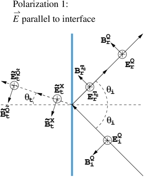
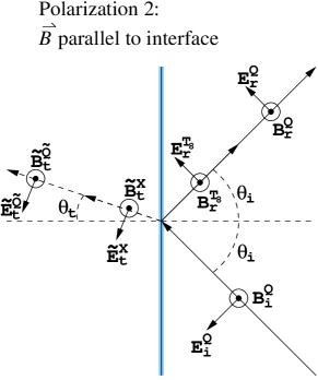
Figure 2: Polarizations of the incident photon beam

III Reflection and Transmission at the Interface

In our analysis we treated both possible polarizations, as illustrated in Fig. 2. Without loss of generality, we assume that the waves incident from $z=+\infty$ will be purely $Q$ gauge bosons. For free phases, two different types of gauge boson may be reflected and/or transmitted. It is also assumed that in a phase where both types of gauge boson are massless, the index of refraction (and hence the $\varepsilon$ and $\mu$) is the same for both.

In addition, the usual rules of optics apply, since they are purely kinematic in nature Jackson . Therefore the angle of reflection equals the angle of incidence, and Snell’s Law applies to the transmitted waves.

To find the transmission and reflection coefficients, we applied the boundary conditions of section II to the kinematic situations shown in Fig. 2. Tables 1 and 2 show the results of these calculations for the eight non-trivial phase combinations. (Some intermediate results, the transmission/reflection amplitudes, are shown and discussed in appendix B).

The shorthand parameters used throughout the calculations are defined as follows:

$$r \equiv \frac{\mu}{\tilde{\mu}}\frac{\tilde{n}}{n}=\sqrt{\frac{\tilde{\varepsilon}\mu}{\varepsilon\tilde{\mu}}},$$ (12)

$$c_{i} \equiv \cos\theta_{i},s_{i}\equiv\sin\theta_{i},$$ (13)

$$c_{t} \equiv \cos\theta_{t},s_{t}\equiv\sin\theta_{t}.$$ (14)

We can eliminate $\cos\theta_{t}$ from the amplitudes by making use of Snell’s Law,

$$n\sin\theta_{i} = \tilde{n}\sin\theta_{t}$$ (15)

$$\to\cos\theta_{t} = \sqrt{1-\frac{n^{2}}{\tilde{n}^{2}}\sin^{2}\!\theta_{i}}.$$ (16)

Reflection and transmission coefficients are defined by

$$R = \frac{I_{r}}{I_{i}}\equiv\frac{\vec{S_{r}}_{\perp}}{\vec{S_{i}}_{\perp}}$$ (17)

$$T = \frac{I_{t}}{I_{i}}\equiv\frac{\vec{S_{t}}_{\perp}}{\vec{S_{i}}_{\perp}}$$ (18)

where $I_{i},I_{r},I_{t}$ refer to the incident, reflected, and transmitted intensities, respectively, and $\vec{S_{i}},\vec{S_{r}},\vec{S_{t}}$ refer to the incident, reflected, and transmitted Poynting vectors; specifically,

$$\begin{array}[]{rclcl}R^{Q}&=&\displaystyle\frac{\hat{z}\cdot\vec{E}^{Q}_{r}\times\vec{H}^{Q}_{r}}{\hat{z}\cdot\vec{E}^{Q}_{i}\times\vec{H}^{Q}_{i}}&=&\displaystyle\frac{c_{r}{{\cal{E}}^{Q}_{r}}^{2}}{c_{i}{{\cal{E}}^{Q}_{i}}^{2}},\\[8.61108pt] R^{T_{8}}&=&\displaystyle\frac{\hat{z}\cdot\vec{E}^{T_{8}}_{r}\times\vec{H}^{T_{8}}_{r}}{\hat{z}\cdot\vec{E}^{Q}_{i}\times\vec{H}^{Q}_{i}}&=&\displaystyle\frac{c_{r}{{\cal{E}}^{T_{8}}_{r}}^{2}}{c_{i}{{\cal{E}}^{T_{8}}_{i}}^{2}},\\[8.61108pt] T^{\tilde{Q}}&=&\displaystyle\frac{\hat{z}\cdot\vec{E}^{\tilde{Q}}_{t}\times\vec{H}^{\tilde{Q}}_{t}}{\hat{z}\cdot\vec{E}^{Q}_{i}\times\vec{H}^{Q}_{i}}&=&\displaystyle\sqrt{\frac{\tilde{\epsilon}\mu}{\epsilon\tilde{\mu}}}\frac{c_{t}{{\cal{E}}^{\tilde{Q}}_{t}}^{2}}{c_{i}{{\cal{E}}^{Q}_{i}}^{2}}.\\[8.61108pt] \end{array}$$ (19)

For clarity, we will illustrate how the calculations leading to tables 1 and 2 are done by looking at two of the cases in detail. The amplitudes ${\cal E}$ give the electric fields associated with the incident, reflected, and transmitted photons,

$$\begin{array}[]{rcl}\vec{E}^{Q}_{i}&=&{\cal{E}}^{Q}_{i}\vec{n}_{i}\exp(i(\vec{k}_{i}\cdot\vec{x}-\omega t))\ ,\\ \vec{E}^{(Q,T_{8})}_{r}&=&{\cal{E}}^{(Q,T_{8})}_{r}\vec{n}_{r}\exp(i(\vec{k}_{r}\cdot\vec{x}-\omega t))\ ,\\ \vec{E}^{\tilde{Q}}_{t}&=&{\cal{E}}^{\tilde{Q}}_{t}\vec{n}_{t}\exp(i(\vec{k}_{t}\cdot\vec{x}-\omega t))\ ,\end{array}$$ (20)

where $\vec{n}$ is the unit polarization vector for each wave.

III.1 $T_{8}$ Free, $X$ Confined

For this combination of phases, the boundary condition equations (8), (9), (10), (11) become

$$D^{Q}_{\perp}(\xi)\begin{pmatrix}1\\ 0\end{pmatrix}+D^{T_{8}}_{\perp}(\xi)\begin{pmatrix}0\\ 1\end{pmatrix}-D^{\tilde{Q}}_{\perp}(-\xi)\begin{pmatrix}\cos\alpha\\ \sin\alpha\end{pmatrix} = 0$$ (21)

$$E^{Q}_{\parallel}(\xi)\begin{pmatrix}1\\ 0\end{pmatrix}+E^{T_{8}}_{\parallel}(\xi)\begin{pmatrix}0\\ 1\end{pmatrix}-E^{\tilde{Q}}_{\parallel}(-\xi)\begin{pmatrix}\cos\alpha\\ \sin\alpha\end{pmatrix} = K^{X}_{M}\begin{pmatrix}-\sin\alpha\\ \phantom{-}\cos\alpha\end{pmatrix}$$ (22)

$$B^{Q}_{\perp}(\xi)\begin{pmatrix}1\\ 0\end{pmatrix}+B^{T_{8}}_{\perp}(\xi)\begin{pmatrix}0\\ 1\end{pmatrix}-B^{\tilde{Q}}_{\perp}(-\xi)\begin{pmatrix}\cos\alpha\\ \sin\alpha\end{pmatrix} = \sigma^{X}_{M}\begin{pmatrix}-\sin\alpha\\ \phantom{-}\cos\alpha\end{pmatrix}$$ (23)

$$H^{Q}_{\parallel}(\xi)\begin{pmatrix}1\\ 0\end{pmatrix}+H^{T_{8}}_{\parallel}(\xi)\begin{pmatrix}0\\ 1\end{pmatrix}-H^{\tilde{Q}}_{\parallel}(-\xi)\begin{pmatrix}\cos\alpha\\ \sin\alpha\end{pmatrix} = 0$$ (24)

Dotting the equations with either ${\begin{pmatrix}\cos\alpha\\ -\sin\alpha\end{pmatrix}}$, $\begin{pmatrix}1\\ 0\end{pmatrix}$, or $\begin{pmatrix}0\\ 1\end{pmatrix}$ as appropriate yields equations that do not depend on the charge or current densities. In this case, we obtain

$$H^{Q}_{\parallel}(\xi) = \cos\alpha H^{\tilde{Q}}_{\parallel}(-\xi)$$ (25)

$$H^{T_{8}}_{\parallel}(\xi) = \sin\alpha H^{\tilde{Q}}_{\parallel}(-\xi)$$ (26)

$$\cos\alpha E^{Q}_{\parallel}(\xi)+\sin\alpha E^{T_{8}}_{\parallel}(\xi) = E^{\tilde{Q}}_{\parallel}(-\xi)$$ (27)

$$\cos\alpha B^{Q}_{\perp}(\xi)+\sin\alpha B^{T_{8}}_{\perp}(\xi) = B^{\tilde{Q}}_{\perp}(-\xi)$$ (28)

For polarization 1 of Fig. 2, equations (25), (26) and (28) lead to

$$rc_{i}({\cal E}^{Q}_{i}-{\cal E}^{Q}_{r}) = \cos\alpha c_{t}{\cal E}^{\tilde{Q}}_{t}$$ (29)

$$-rc_{i}{\cal E}^{T_{8}}_{r} = \sin\alpha c_{t}{\cal E}^{\tilde{Q}}_{t}$$ (30)

$$\cos\alpha({\cal E}^{Q}_{i}+{\cal E}^{Q}_{r})+\sin\alpha{\cal E}^{T_{8}}_{r} = {\cal E}^{\tilde{Q}}_{t}$$ (31)

which can be solved for the amplitudes in Table 4, row 5. Using (17) and (19) we obtain the reflection/transmission coefficients of Table 1, row 5.

For polarization 2 of Fig. 2, equations (25), (26) and (27) lead to

$$r({\cal E}^{Q}_{i}+{\cal E}^{Q}_{r}) = \cos\alpha{\cal E}^{\tilde{Q}}_{t}$$ (32)

$$r{\cal E}^{T_{8}}_{r} = \sin\alpha{\cal E}^{\tilde{Q}}_{t}$$ (33)

$$c_{i}(\cos\alpha({\cal E}^{Q}_{i}-{\cal E}^{Q}_{r})-\sin\alpha{\cal E}^{T_{8}}_{r}) = c_{t}{\cal E}^{\tilde{Q}}_{t}$$ (34)

which can similarly be solved for the amplitudes in Table 5, row 5, and reflection/transmission coefficients in Table 2, row 5.

III.2 $T_{8}$ Higgsed, $X$ Higgsed

When there is Higgsing in both regions, the boundary condition equations (8)-(11) become

$$D^{Q}_{\perp}(\xi)\begin{pmatrix}1\\ 0\end{pmatrix}-D^{\tilde{Q}}_{\perp}(-\xi)\begin{pmatrix}\cos\alpha\\ \sin\alpha\end{pmatrix} = \sigma^{T_{8}}\begin{pmatrix}0\\ 1\end{pmatrix}+\sigma^{X}\begin{pmatrix}-\sin\alpha\\ \phantom{-}\cos\alpha\end{pmatrix}$$ (35)

$$E^{Q}_{\parallel}(\xi)\begin{pmatrix}1\\ 0\end{pmatrix}-E^{\tilde{Q}}_{\parallel}(-\xi)\begin{pmatrix}\cos\alpha\\ \sin\alpha\end{pmatrix} = 0$$ (36)

$$B^{Q}_{\perp}(\xi)\begin{pmatrix}1\\ 0\end{pmatrix}-B^{\tilde{Q}}_{\perp}(-\xi)\begin{pmatrix}\cos\alpha\\ \sin\alpha\end{pmatrix} = 0$$ (37)

$$H^{Q}_{\parallel}(\xi)\begin{pmatrix}1\\ 0\end{pmatrix}-H^{\tilde{Q}}_{\parallel}(-\xi)\begin{pmatrix}\cos\alpha\\ \sin\alpha\end{pmatrix} = K^{T_{8}}\begin{pmatrix}0\\ 1\end{pmatrix}+K^{X}\begin{pmatrix}-\sin\alpha\\ \phantom{-}\cos\alpha\end{pmatrix}$$ (38)

In this case, we find

$$E^{Q}_{\parallel}(\xi) = E^{\tilde{Q}}_{\parallel}(-\xi)=0$$ (39)

$$B^{Q}_{\perp}(\xi) = B^{\tilde{Q}}_{\perp}(-\xi)=0$$ (40)

For polarization 1 of Fig. 2, either equation (39) or (40) leads to the simple equations

$${\cal E}^{Q}_{i}+{\cal E}^{Q}_{r} = 0$$ (41)

$${\cal E}^{\tilde{Q}}_{t} = 0$$ (42)

which shows that waves of this polarization are completely reflected with a 180 degree phase shift.

For polarization 2 of Fig. 2, either equation (39) or (40) leads to the equally simple equations

$${\cal E}^{Q}_{r}-{\cal E}^{Q}_{i} = 0$$ (43)

$${\cal E}^{\tilde{Q}}_{t} = 0$$ (44)

which shows that waves of this polarization are completely reflected with no phase shift.

Table 1: Reflection and Transmission Coefficients for Polarization 1. For definitions see (12): $c_{i}$ and $c_{t}$ are the cosines of the incident and transmitted beams; $\alpha$ is the mismatch between the generators of the free $U(1)$’s in the outside region ($Q$) and the inside region (${\tilde{Q}}$); $r$ is a function of the permittivities and permeabilities of the two regions.

Outer region ($T_{8})$	Inner region ($X$)	$R^{Q}$	$R^{T_{8}}$	$T^{\tilde{Q}}$	$T^{X}$
Higgsed	Higgsed	$1$	0	0	0
Confined	Confined	$1$	0	0	0
Free	Higgsed	$\displaystyle{\left(\frac{c_{i}\cos 2\alpha-rc_{t}}{c_{i}+rc_{t}}\right)^{2}}$	$\displaystyle{\left(\frac{c_{i}\sin 2\alpha}{c_{i}+rc_{t}}\right)^{2}}$	$\displaystyle{\frac{4rc_{i}c_{t}\cos^{2}\!\alpha}{(c_{i}+rc_{t})^{2}}}$	0
Higgsed	Free	$\displaystyle{\left(\frac{c_{i}-rc_{t}}{c_{i}+rc_{t}}\right)^{2}}$	0	$\displaystyle{\frac{4rc_{i}c_{t}\cos^{2}\!\alpha}{(c_{i}+rc_{t})^{2}}}$	$\displaystyle{\frac{4rc_{i}c_{t}\sin^{2}\!\alpha}{(c_{i}+rc_{t})^{2}}}$
Free	Confined	$\displaystyle{\left(\frac{c_{i}-rc_{t}\cos 2\alpha}{c_{i}+rc_{t}}\right)^{2}}$	$\displaystyle{\left(\frac{rc_{t}\sin 2\alpha}{c_{i}+rc_{t}}\right)^{2}}$	$\displaystyle{\frac{4rc_{i}c_{t}\cos^{2}\!\alpha}{(c_{i}+rc_{t})^{2}}}$	0
Confined	Free	$\displaystyle{\left(\frac{c_{i}-rc_{t}}{c_{i}+rc_{t}}\right)^{2}}$	0	$\displaystyle{\frac{4rc_{i}c_{t}\cos^{2}\!\alpha}{(c_{i}+rc_{t})^{2}}}$	$\displaystyle{\frac{4rc_{i}c_{t}\sin^{2}\!\alpha}{(c_{i}+rc_{t})^{2}}}$
Higgsed	Confined	$\displaystyle{\left(\frac{c_{i}-rc_{t}\cos^{2}\!\alpha}{c_{i}+rc_{t}\cos^{2}\!\alpha}\right)^{2}}$	0	$\displaystyle{\frac{4rc_{i}c_{t}\cos^{2}\!\alpha}{(c_{i}+rc_{t}\cos^{2}\!\alpha)^{2}}}$	0
Confined	Higgsed	$\displaystyle{\left(\frac{c_{i}\cos^{2}\!\alpha-rc_{t}}{c_{i}\cos^{2}\!\alpha+rc_{t}}\right)^{2}}$	0	$\displaystyle{\frac{4rc_{i}c_{t}\cos^{2}\!\alpha}{(c_{i}\cos^{2}\!\alpha+rc_{t})^{2}}}$	0

Table 2: Reflection and Transmission Coefficients for Polarization 2

Outer region ($T_{8})$	Inner region ($X$)	$R^{Q}$	$R^{T_{8}}$	$T^{\tilde{Q}}$	$T^{X}$
Higgsed	Higgsed	$1$	0	0	0
Confined	Confined	$1$	0	0	0
Free	Higgsed	$\displaystyle{\left(\frac{rc_{i}-c_{t}\cos 2\alpha}{rc_{i}+c_{t}}\right)^{2}}$	$\displaystyle{\left(\frac{c_{t}\sin 2\alpha}{rc_{i}+c_{t}}\right)^{2}}$	$\displaystyle{\frac{4rc_{i}c_{t}\cos^{2}\!\alpha}{(rc_{i}+c_{t})^{2}}}$	0
Higgsed	Free	$\displaystyle{\left(\frac{rc_{i}-c_{t}}{rc_{i}+c_{t}}\right)^{2}}$	0	$\displaystyle{\frac{4rc_{i}c_{t}\cos^{2}\!\alpha}{(rc_{i}+c_{t})^{2}}}$	$\displaystyle{\frac{4rc_{i}c_{t}\sin^{2}\!\alpha}{(rc_{i}+c_{t})^{2}}}$
Free	Confined	$\displaystyle{\left(\frac{rc_{i}\cos 2\alpha-c_{t}}{rc_{i}+c_{t}}\right)^{2}}$	$\displaystyle{\left(\frac{rc_{i}\sin 2\alpha}{rc_{i}+c_{t}}\right)^{2}}$	$\displaystyle{\frac{4rc_{i}c_{t}\cos^{2}\!\alpha}{(rc_{i}+c_{t})^{2}}}$	0
Confined	Free	$\displaystyle{\left(\frac{rc_{i}-c_{t}}{rc_{i}+c_{t}}\right)^{2}}$	0	$\displaystyle{\frac{4rc_{i}c_{t}\cos^{2}\!\alpha}{(rc_{i}+c_{t})^{2}}}$	$\displaystyle{\frac{4rc_{i}c_{t}\sin^{2}\!\alpha}{(rc_{i}+c_{t})^{2}}}$
Higgsed	Confined	$\displaystyle{\left(\frac{rc_{i}\cos^{2}\!\alpha-c_{t}}{rc_{i}\cos^{2}\!\alpha+c_{t}}\right)^{2}}$	0	$\displaystyle{\frac{4rc_{i}c_{t}\cos^{2}\!\alpha}{(rc_{i}\cos^{2}\!\alpha+c_{t})^{2}}}$	0
Confined	Higgsed	$\displaystyle{\left(\frac{rc_{i}-c_{t}\cos^{2}\!\alpha}{rc_{i}+c_{t}\cos^{2}\!\alpha}\right)^{2}}$	0	$\displaystyle{\frac{4rc_{i}c_{t}\cos^{2}\!\alpha}{(rc_{i}+c_{t}\cos^{2}\!\alpha)^{2}}}$	0

IV Summary and Discussion

We have studied reflection and transmission of gauge bosons at the interface between differently realized phases of a $U(1)\otimes U(1)$ gauge theory. In order to allow gauge bosons to propagate, at least one linear combination of the gauge generators must be free on each side of the interface: this is taken to be $Q$ in the outer region ($z>0$) and ${\tilde{Q}}$ in the inner region ($z<0$). The other generator is $T_{8}$ in the outer region and $X$ in the inner region. The possibilities for this other generator are that it can be also free, Higgsed, or confined. The $(Q,T_{8})$ basis may in general be rotated by an angle $\alpha$ relative to the $({\tilde{Q}},X)$ basis. Since the Free/Free boundary ($T_{8}$ free outside, $X$ free inside) is trivial for any $\alpha$, this means that there are 8 possible types of boundary. The transmission and reflection coefficients for light arriving at these different types of boundary are given in Tables 1 and 2. These are complicated so we give a qualitative summary in table 3, and we will now discuss the entries in that table.

IV.1 How the different boundaries behave

Table 3: Behavior of gauge bosons at an interface in $U(1)\otimes U(1)$ gauge theory for various realizations of the gauge symmetries on each side. The gauge bosons are assumed to arrive as $Q$-photons from the “outer” phase.

		Inner ($z<0$), ${\tilde{Q}}$ free
		$X$ Free	$X$ Higgsed	$X$ Confined
	$T_{8}$ Free	transmission	$Q,T_{8}$ reflection ${\tilde{Q}}$ transmission	$Q,T_{8}$ reflection ${\tilde{Q}}$ transmission
Outer ($z>0$) $Q$ free	$T_{8}$ Higgsed	$Q$ reflection ${\tilde{Q}},X$ transmission	total reflection	$Q$ reflection ${\tilde{Q}}$ transmission
	$T_{8}$ Confined	$Q$ reflection ${\tilde{Q}},X$ transmission	$Q$ reflection ${\tilde{Q}}$ transmission	total reflection

If all generators everywhere are free ($T_{8}$ and $X$ both free, row 1 column 1 of table 3), then there is no distinction between the inner and outer regions other than a possible difference in refractive index, so there will be transmission and reflection as at a dielectric boundary like a glass-air boundary.

If both generators in the outer region are free ($T_{8}$ free) but in the inner region $X$ is Higgsed or confined (row 1 columns 2 and 3 of table 3), then the gauge bosons are partially reflected and partially transmitted, depending on the angle between ${\tilde{Q}}$ and $Q$. However, even though the incident wave is pure $Q$ gauge bosons, there will be some additional $T_{8}$ bosons created and reflected back. The transmitted wave will be pure ${\tilde{Q}}$ gauge bosons. Similarly, if both generators in the inner region are free ($X$ is free) and in the outer region $T_{8}$ is Higgsed or confined (column 1 rows 2 and 3 of table 3) then there will be transmission of both ${\tilde{Q}}$ and $X$, adding up to make a $Q$-photon.

If there is only one free generator in each region, $Q$ on the outside and ${\tilde{Q}}$ on the inside, then the reflected wave must be pure $Q$-photons and the transmitted wave must be pure ${\tilde{Q}}$ photons. If the broken generator is Higgsed on one side and confined on the other then there is partial reflection and partial transmission (row 2 column 3 and column 3 row 2 of table 3). This was the case studied in manraj .

If the broken generators on the inside and outside are both Higgsed, or both confined then the behavior is very different. Electromagnetic waves are completely reflected at an interface between two Higgsed phases with different values of $\alpha$ (row 2 column 2 of table 3) or between two confined phases where the confined gauge fields are different linear combinations of $Q$ and $T_{8}$ (row 3 column 3 of table 3). In addition, since one polarization is flipped in each case while the other stays the same, left circularly polarized waves are reflected as right circularly polarized waves, and vice versa. This raises an interesting puzzle: the Higgs/Higgs and confined/confined boundaries both show total reflection independent of the value of $\alpha$. But when $\alpha=0$ both phases have identical unbroken gauge generators, so the interface is just a boundary between two media with different dielectric constants, and there should be some transmission. In fact, in the limit $(\tilde{\epsilon},\tilde{\mu})\to(\epsilon,\mu)$ there is no boundary, and there must be total transmission. This paradox is analyzed below.

IV.2 Compatibility with previous results

In Ref. manraj , Manuel and Rajagopal studied the case where $X$ is Higgsed on the inside and $T_{8}$ is confined on the outside, and our results for that case agree with theirs. One of their main conclusions was that it is possible to use light reflection calculations to show that there are magnetic monopoles in the QCD vacuum. Their argument was that the situation they studied corresponds to the boundary between the confining QCD vacuum and color-superconducting quark matter, and for that situation they derived the confining boundary condition for $T_{8}$ color-magnetic flux, which tells us there are $T_{8}$ magnetic monopoles in the boundary region, from a few basic assumptions, namely: (1) color is not Higgsed, so there are no color ($T_{8}$) supercurrents in the boundary layer; (2) no gluons (ie $T_{8}$ gauge bosons) propagate in the confined phase; (3) conservation of energy; (4) Snell’s law for the angles of reflection and transmission.

This result can be obtained more directly, without using light reflection calculations, from considerations of static electromagnetic fields at an interface using assumptions (1) and (2) alone. Consider what must happen to ${\tilde{Q}}$ magnetic flux lines that arrive at the boundary from the quark matter side. Their $T_{8}$ component cannot penetrate into the QCD vacuum region, since color is confined there (assumption (2)), and they cannot be turned back into the quark matter region by the Meissner effect because there are no $T_{8}$ supercurrents in the boundary layer (assumption (1)). So the flux lines have to end. This means that at the edge of a color-confined phase there must be a boundary layer of color magnetic monopoles that eat up any unwanted color magnetic flux that might try to enter the confined region.

IV.3 The singular $\alpha\to 0$ limit

We now turn to the paradoxical behavior of the Higgsed/Higgsed and confined/confined interfaces, which seem to always reflect all light even in the limit $\alpha\to 0$, where the interface becomes a typical dielectric boundary which ought to transmit at least some light. To understand this we have to be careful about specifying the wavelength of the light that is incident on the boundary.

As mentioned in section II, throughout our calculations we have worked in the limit of long wavelength relative to the penetration depth, $\lambda\gg\xi$. This corresponds to the low frequency limit, $\omega\ll c/\xi$. It turns out that, for the Higgsed/Higgsed and confined/confined interfaces, the limit of low frequency does not commute with the limit $\alpha\to 0$ in which the unbroken $U(1)$’s on either side of the boundary become the same. An explicit calculation for the Higgs-Higgs boundary at finite $\alpha$ and $\omega$ is given in Appendix A.

We can summarize the result as follows. For polarization 1 (the argument for polarization 2 is analogous) the transmission amplitude at low frequency ($\omega\xi\ll c$) and small $\alpha$ is of the form

$$\frac{\omega\xi}{\omega\xi+i\alpha^{2}c}$$ (45)

where $\xi$ is the penetration depth, and dimensionless factors of order one (cosines of angles, etc) have been omitted. In the limit where $\omega\to 0$ first, $\omega\xi\ll\alpha^{2}c\ll c$, the transmission amplitude is zero: this is the total reflection expressed in the first two rows of tables 1 and 2. In the limit where $\alpha\to 0$ first, $\alpha^{2}c\ll\omega\xi\ll c$, the transmission amplitude is of order 1: this is what we expect when there is no mismatch between the unbroken $U(1)$’s at the boundary. We conclude that the paradox is resolved in this way: at small $\alpha$ there is total reflection for frequencies below $\alpha^{2}c/\xi$, but higher frequencies are transmitted. As $\alpha\to 0$ the range of reflected frequencies becomes smaller and smaller, and finally disappears.

For most of the boundaries we studied, the two limits commute, and we can, without ambiguity, work at arbitrarily low frequency, and discuss how the reflection and transmission depend on $\alpha$. But for the Higgs/Higgs and confined/confined boundaries the order of the limits must be specified.

IV.4 Complementarity

The complementarity principle complementarity states that for any Higgsed description of a gauge theory there should be a corresponding confined description, so that there is no way to distinguish a confined phase from a Higgs phase. Since the Higgs phase involves condensation of electrically charged fields, while the confined phase involves condensation of magnetically charged fields, we expect that the confined$\,\rightleftharpoons\,$Higgs mapping will involve a magnetic$\,\rightleftharpoons\,$electric duality transformation. Exchanging magnetic and electric fields converts polarization 1 into polarization 2 (see Fig. 2), so the confined$\,\rightleftharpoons\,$Higgs mapping will be

$$\begin{array}[]{rcl@{\qquad\quad}rcl}\vec{E}&\to&\vec{H},&\vec{H}\to-\vec{E},\\ \vec{D}&\to&\vec{B},&\vec{B}\to-\vec{D},\\ q_{e}&\to&q_{m},&q_{m}\to-q_{e},\\ \vec{J}_{e}&\to&\vec{J}_{m},&\vec{J}_{m}\to-\vec{J}_{e},\\ \lx@intercol\hfil\tilde{\epsilon}\rightleftharpoons\tilde{\mu},\hfil\lx@intercol\\ \lx@intercol\hfil r\rightleftharpoons 1/r\hfil\lx@intercol\\ \lx@intercol\hfil\mbox{polarization 1}\rightleftharpoons\mbox{polarization 2}\hfil\lx@intercol\\ \lx@intercol\hfil\mbox{Higgsed}\rightleftharpoons\mbox{Confined}\hfil\lx@intercol\\ \end{array}$$ (46)

Since the reflection and transmission coefficients are related to the energy and momentum flow in the scattering process, they are directly observable, and should be invariant under the duality transformation (46). Inspecting tables 1 and 2 we see that this is indeed the case. For example, the reflection and transmission coefficients for the Higgsed-Free boundary (third line of table 1) are transformed into those for the Confined-Free boundary (fifth line in table 2). In other words, if we shine light on a boundary and obtain the results of table 1 line 3, then we could not distinguish whether the outside phase is Higgsed or confined.

This means that by measuring only the reflected and transmitted indensities, we can only distinguish 4 of the 8 types of non-trivial boundary. What is clear from tables 1 and 2 is that this ambiguity only exists as a single global choice. There is not a separate confined vs. Higgs choice for each phase independently. This is exactly what we expect from the principle of complementarity.

One might naively think that it should be possible to overcome this ambiguity by measuring the electric and magnetic fields (which are also gauge-invariant and physically measureable) directly. Carefully constructing the corresponding thought-experiment shows that this does not in fact overcome the ambiguity: we discuss this in appendix B.

IV.5 Future directions

As mentioned in the introduction, the $U(1)\otimes U(1)$ system arises in various contexts within particle physics, and the results of this paper may be applied to domain walls or phase boundaries in those contexts. The same formalism can also be used for more general gauge groups, as in the work of Manuel and Rajagopal manraj . Quark matter provides a possible area of application, since it has a rich phase diagram, including a variety of patterns of confinement or Higgsing of various subgroups of the $SU(3)_{\rm color}\otimes U(1)_{Q}$ gauge group Reviews .

Finally, in our analysis we only concerned ourselves with the gauge symmetries, not with any global symmetries. If massless fermionic fields are included in the theory then chiral symmetry complicates the complementarity principle complementarity_with_fermions . It would be interesting to see how this affects the distinguishability of our $U(1)\otimes U(1)$ interfaces. One immediate question is the contradiction between Ref. complementarity_with_fermions , which predicts that chiral symmetries will not not be broken in weakly-coupled Higgsed phases, and the accepted picture of high-density quark matter, according to which CFL pairing produces Higgs breaking of the color gauge symmetry and simultaneously breaks chiral symmetry. This is crucial to the concept of quark-hadron continuity, which identifies the CFL phase as a controlled continuation of the confined phase.

Appendix A Non-zero-frequency effects

The macroscopic calculations of section II are performed under the simplifying assumption that the frequencies are very small, and therefore the time-derivative terms in the Maxwell equations are neglected. It is also assumed that the Higgsed or confined fields are quickly screened, so the field amplitudes are set to zero from the beginning. The advantage of this approach is that the spatial behavior of the screened fields and the screening currents does not have to be determined, so the solution is straightforward. However, any finite frequency effects are thrown away, and as mentioned in section IV.3, Higgsed/Higgsed and confined/confined interfaces have singular behavior in the $\alpha\to 0$ limit. To rectify this problem, we performed the calculation again for the Higgsed/Higgsed combination, keeping the contributions of screened fields and finite frequency.

First, we briefly review the behavior of electromagnetic fields in a superconductor. In addition to the Maxwell equations (5), we have the London equations (see Ref. ashcroftmermin , chapter 34)

$$\frac{d\vec{J}}{dt} = \gamma\vec{E},$$

$$\vec{\nabla}\times\vec{J} = -\gamma\vec{B}$$ (47)

that describe how the supercurrents respond to applied fields. The parameter $\gamma$ depends on microscopic details such as the density and charge of Cooper pairs that make up the supercurrents, but the details are not important for this discussion. Inserting equations (A) into the “curl” equation for $\vec{B}$, we obtain the wave equation for the magnetic field in the superconductor,

$$\nabla^{2}\vec{B}=\mu\gamma\vec{B}+\frac{1}{c^{2}}\frac{\partial^{2}\vec{B}}{\partial t^{2}}$$ (48)

From dimensional considerations the definition of the screening length $\xi$ is defined as

$$\xi\equiv\frac{1}{\sqrt{\mu\gamma}}$$ (49)

and the solutions of the wave equation have the form

$$\vec{B}=\vec{B_{0}}\exp\left[\vec{\kappa}\cdot\vec{x}-i\omega t\right].$$ (50)

Plugging this solution back into the wave equation obtains the magnitude of the wavevector,

$$|\kappa|=\pm\sqrt{\frac{1}{\xi^{2}}-\frac{\omega^{2}}{c^{2}}}.$$ (51)

For frequencies less than $c/\xi$, the waves are completely damped, while for frequencies greater than $c/\xi$, the waves propagate without any damping. For $\omega=c/\xi$, the wave has no spatial variation and only oscillates in time. The choice of the positive or negative solution for the wavevector depends on the boundary conditions of the superconducting phase. We can obtain identical wave equations for $\vec{J}$ and $\vec{E}$; since we are still interested in the low-frequency limit, we can use the limiting value $|\kappa|=\pm\xi^{-1}$ to obtain the magnitudes of the current and the electric field as

$$|J_{0}|=\mp\xi\gamma|B_{0}|,$$

$$|E_{0}|=\pm i\omega\xi|B_{0}|$$ (52)

For the Higgsed/Higgsed phase combination, the Higgsed fields on either side of the boundary will satisfy the equations above. Explicitly, we have

$$\vec{E}^{Q}_{i} = {\cal{E}}^{Q}_{i}\vec{n}_{i}\exp(i(\vec{k}_{i}\cdot\vec{x}-\omega t))\ ,$$

$$\vec{E}^{Q}_{r} = {\cal{E}}^{Q}_{r}\vec{n}_{r}\exp(i(\vec{k}_{r}\cdot\vec{x}-\omega t))\ ,$$

$$\vec{E}^{T_{8}}_{r} = {\cal{E}}^{T_{8}}_{r}\vec{n}_{r}\exp(-\vec{\kappa}_{r}\cdot\vec{x}-i\omega t)\ ,$$

$$\vec{E}^{\tilde{Q}}_{t} = {\cal{E}}^{\tilde{Q}}_{t}\vec{n}_{t}\exp(i(\vec{k}_{t}\cdot\vec{x}-\omega t)),$$

$$\vec{E}^{X}_{t} = {\cal{E}}^{X}_{t}\vec{n}_{t}\exp(+\vec{\kappa}_{t}\cdot\vec{x}-i\omega t))\ ,$$ (53)

The “${\cal{E}}$” amplitudes are the magnitudes of the electric field at the boundary itself ($z=0$); all screening is due to the spatial terms.

Now we will rewrite the boundary condition equations keeping everything that was thrown away previously. The “curl” equations are sufficient to solve for the field amplitudes. We obtain

$$E^{Q}_{\parallel}\begin{pmatrix}1\\ 0\end{pmatrix}+E^{T_{8}}_{\parallel}\begin{pmatrix}0\\ 1\end{pmatrix}-E^{\tilde{Q}}_{\parallel}\begin{pmatrix}\cos\alpha\\ \sin\alpha\end{pmatrix}-E^{X}_{\parallel}\begin{pmatrix}-\sin\alpha\\ \phantom{-}\cos\alpha\end{pmatrix}$$

$$=\frac{i\omega}{\kappa_{z}}B^{T_{8}}_{\parallel}\begin{pmatrix}0\\ 1\end{pmatrix}+\frac{i\omega}{\tilde{\kappa}_{z}}B^{X}_{\parallel}\begin{pmatrix}-\sin\alpha\\ \phantom{-}\cos\alpha\end{pmatrix}$$ (54)

$$B^{Q}_{\parallel}\begin{pmatrix}1\\ 0\end{pmatrix}+\left(1-\frac{1}{\xi\kappa_{z}}\right)B^{T_{8}}_{\parallel}\begin{pmatrix}0\\ 1\end{pmatrix}-B^{\tilde{Q}}_{\parallel}\begin{pmatrix}\cos\alpha\\ \sin\alpha\end{pmatrix}$$

$$\makebox[30.00005pt]{~{}}-\left(1+\frac{1}{\tilde{\xi}\tilde{\kappa}_{z}}\right)B^{X}_{\parallel}\begin{pmatrix}-\sin\alpha\\ \phantom{-}\cos\alpha\end{pmatrix}$$

$$=-\frac{i\omega}{c^{2}\kappa_{z}}E^{T_{8}}_{\parallel}\begin{pmatrix}0\\ 1\end{pmatrix}-\frac{i\omega}{\tilde{c}^{2}\tilde{\kappa}_{z}}E^{X}_{\parallel}\begin{pmatrix}-\sin\alpha\\ \phantom{-}\cos\alpha\end{pmatrix}$$ (55)

For polarization 1 of Figure 2, the solutions for the amplitudes are

$$\begin{array}[]{rcl}\displaystyle\frac{{\cal E}^{Q}_{r}}{{\cal E}^{Q}_{i}}&=&\displaystyle\frac{\omega\tilde{\xi}(c_{i}-\cos^{2}\!\alpha\frac{\tilde{n}}{n}c_{t})+ic(1+c_{t})\sin^{2}\!\alpha}{\omega\tilde{\xi}(c_{i}+\cos^{2}\!\alpha\frac{\tilde{n}}{n}c_{t})-ic(1+c_{t})\sin^{2}\!\alpha}\\[12.91663pt] \displaystyle\frac{{\cal E}^{T_{8}}_{r}}{{\cal E}^{Q}_{i}}&=&\displaystyle\frac{\sin 2\alpha\omega\xi c_{i}(1+c_{t})}{\omega\tilde{\xi}(c_{i}+\cos^{2}\!\alpha\frac{\tilde{n}}{n}c_{t})-ic(1+c_{t})\sin^{2}\!\alpha}\\[12.91663pt] \displaystyle\frac{{\cal E}^{\tilde{Q}}_{t}}{{\cal E}^{Q}_{i}}&=&\displaystyle\frac{2\cos\alpha\omega\tilde{\xi}c_{i}}{\omega\tilde{\xi}(c_{i}+\cos^{2}\!\alpha\frac{\tilde{n}}{n}c_{t})-ic(1+c_{t})\sin^{2}\!\alpha}\\[12.91663pt] \displaystyle\frac{{\cal E}^{X}_{t}}{{\cal E}^{Q}_{i}}&=&\displaystyle\frac{2\sin\alpha\omega\tilde{\xi}c_{i}}{\omega\tilde{\xi}(c_{i}+\cos^{2}\!\alpha\frac{\tilde{n}}{n}c_{t})-ic(1+c_{t})\sin^{2}\!\alpha}.\end{array}$$ (56)

Taking the $\omega\to 0$ limit, we recover the amplitudes of the first row of Table 4 presented below in Appendix B. However, more importantly, taking the $\alpha\to 0$ limit first, we obtain

$${\cal E}^{Q}_{r} = {\cal E}^{Q}_{i}\left[\frac{c_{i}-\frac{\tilde{n}}{n}c_{t}}{c_{i}+\frac{\tilde{n}}{n}c_{t}}\right]$$

$${\cal E}^{T_{8}}_{r} \to 0$$

$${\cal E}^{\tilde{Q}}_{t} = {\cal E}^{Q}_{i}\left[\frac{2c_{i}}{c_{i}+\frac{\tilde{n}}{n}c_{t}}\right]$$

$${\cal E}^{X}_{t} \to 0,$$ (57)

which are the normal reflection and refraction amplitudes from electrodynamics. Similarly, for polarization 2 of Figure 2, the solutions for the amplitudes are

$$\begin{array}[]{rcl}\displaystyle\frac{{\cal E}^{Q}_{r}}{{\cal E}^{Q}_{i}}&=&\displaystyle\frac{2\omega\left[\xi(1+c_{i}^{2})(1+c_{t})(\frac{\tilde{n}}{n}c_{i}-\cos^{2}\!\alpha c_{t})-\tilde{\xi}(1+c_{i})(1+c_{t}^{2})(\cos^{2}\!\alpha\frac{\tilde{n}}{n}c_{i}-c_{t})\right]+2i\sin^{2}\!\alpha cc_{i}c_{t}(1+c_{i})(1+c_{t})}{2\omega\left[\xi(1+c_{i}^{2})(1+c_{t})(\frac{\tilde{n}}{n}c_{i}+\cos^{2}\!\alpha c_{t})-\tilde{\xi}(1+c_{i})(1+c_{t}^{2})(\cos^{2}\!\alpha\frac{\tilde{n}}{n}c_{i}+c_{t})\right]+2i\sin^{2}\!\alpha cc_{i}c_{t}(1+c_{i})(1+c_{t})}\\[12.91663pt] \displaystyle\frac{{\cal E}^{T_{8}}_{r}}{{\cal E}^{Q}_{i}}&=&\displaystyle\frac{-2\omega\xi\sin 2\alpha c_{i}^{2}c_{t}(1+c_{t})}{2\omega\left[\xi(1+c_{i}^{2})(1+c_{t})(\frac{\tilde{n}}{n}c_{i}+\cos^{2}\!\alpha c_{t})-\tilde{\xi}(1+c_{i})(1+c_{t}^{2})(\cos^{2}\!\alpha\frac{\tilde{n}}{n}c_{i}+c_{t})\right]+2i\sin^{2}\!\alpha cc_{i}c_{t}(1+c_{i})(1+c_{t})}\\[12.91663pt] \displaystyle\frac{{\cal E}^{\tilde{Q}}_{t}}{{\cal E}^{Q}_{i}}&=&\displaystyle\frac{4\omega\cos\alpha c_{i}\left[\xi(1+c_{i}^{2})(1+c_{t})-\tilde{\xi}(1+c_{i})(1+c_{t}^{2})\right]}{2\omega\left[\xi(1+c_{i}^{2})(1+c_{t})(\frac{\tilde{n}}{n}c_{i}+\cos^{2}\!\alpha c_{t})-\tilde{\xi}(1+c_{i})(1+c_{t}^{2})(\cos^{2}\!\alpha\frac{\tilde{n}}{n}c_{i}+c_{t})\right]+2i\sin^{2}\!\alpha cc_{i}c_{t}(1+c_{i})(1+c_{t})}\\[12.91663pt] \displaystyle\frac{{\cal E}^{X}_{t}}{{\cal E}^{Q}_{i}}&=&\displaystyle\frac{4\omega\tilde{\xi}\sin\alpha c_{i}(1+c_{i})c_{t}^{2}}{2\omega\left[\xi(1+c_{i}^{2})(1+c_{t})(\frac{\tilde{n}}{n}c_{i}+\cos^{2}\!\alpha c_{t})-\tilde{\xi}(1+c_{i})(1+c_{t}^{2})(\cos^{2}\!\alpha\frac{\tilde{n}}{n}c_{i}+c_{t})\right]+2i\sin^{2}\!\alpha cc_{i}c_{t}(1+c_{i})(1+c_{t})}.\end{array}$$ (58)

Once again, taking the $\omega\to 0$ limit, we recover the amplitudes of the first row of Table 5 presented below in Appendix B. Taking the $\alpha\to 0$ limit first, we obtain

$${\cal E}^{Q}_{r} = {\cal E}^{Q}_{i}\left[\frac{\frac{\tilde{n}}{n}c_{i}-c_{t}}{\frac{\tilde{n}}{n}c_{i}+c_{t}}\right]$$

$${\cal E}^{T_{8}}_{r} \to 0$$

$${\cal E}^{\tilde{Q}}_{t} = {\cal E}^{Q}_{i}\left[\frac{2c_{i}}{\frac{\tilde{n}}{n}c_{i}+c_{t}}\right]$$

$${\cal E}^{X}_{t} \to 0,$$ (59)

the normal reflection and refraction amplitudes for perpedicularly polarized light.

This shows that our “singular” limit problem is actually an order-of-limits problem. For most of the possible phase combinations, we could take the $\omega\to 0$ limit at the beginning and not encounter any problems, but for the Higgsed/Higgsed or confined/confined phases, that is incorrect. Although the frequency drops out in the $\alpha\to 0$ limit, we need to keep a nonzero frequency value to obtain the correct expression.

Appendix B Field strengths and complementarity

In tables 4 and 5 we show the reflection and transmission amplitudes, i.e. the ratios between electric field strengths in the incident, reflected, and transmitted beams. It is clear that the transmission amplitudes do not show invariance under the duality transformation (46). Does this mean that measurements of electric and magnetic fields can overcome the complementarity ambiguity and distinguish a Higgsed phase from a confined phase? In this appendix, we show that although electric and magnetic fields are gauge-invariant quantities, what can actually be measured is the force exerted on a charge, so that even experiments that seem to directly measure field strengths suffer from the Higgsed/confined ambiguity.

For illustrative purposes, we calculate the Lorentz force on a test charge in the inner phase due to electromagnetic waves transmitted from the outer phase. First, we will calculate the force in the case where the outer phase is confined and the inner phase is Higgsed; then we will calculate the force in the dual picture, where the outer phase is Higgsed and the inner phase is confined. We will see that although the transmission amplitudes are not invariant under the duality transformation, the physically measureable quantity, force, is invariant.

Table 4: Reflected and Transmitted Amplitudes for Polarization 1

Outer region ($T_{8})$	Inner region ($X$)	${\cal E}^{Q}_{r}/{\cal E}^{Q}_{i}$	${\cal E}^{T_{8}}_{r}/{\cal E}^{Q}_{i}$	${\cal E}^{\tilde{Q}}_{t}/{\cal E}^{Q}_{i}$	${\cal E}^{X}_{t}/{\cal E}^{Q}_{i}$
Higgsed	Higgsed	$-1$	0	0	0
Confined	Confined	$1$	0	0	0
Free	Higgsed	$\displaystyle{\frac{c_{i}\cos 2\alpha-rc_{t}}{c_{i}+rc_{t}}}$	$\displaystyle{\frac{c_{i}\sin 2\alpha}{c_{i}+rc_{t}}}$	$\displaystyle{\frac{2c_{i}\cos\alpha}{c_{i}+rc_{t}}}$	0
Higgsed	Free	$\displaystyle{\frac{c_{i}-rc_{t}}{c_{i}+rc_{t}}}$	0	$\displaystyle{\frac{2c_{i}\cos\alpha}{c_{i}+rc_{t}}}$	$\displaystyle{\frac{-2c_{i}\sin\alpha}{c_{i}+rc_{t}}}$
Free	Confined	$\displaystyle{\frac{c_{i}-rc_{t}\cos 2\alpha}{c_{i}+rc_{t}}}$	$\displaystyle{\frac{-rc_{t}\sin 2\alpha}{c_{i}+rc_{t}}}$	$\displaystyle{\frac{2c_{i}\cos\alpha}{c_{i}+rc_{t}}}$	0
Confined	Free	$\displaystyle{\frac{c_{i}-rc_{t}}{c_{i}+rc_{t}}}$	0	$\displaystyle{\frac{2c_{i}\cos\alpha}{c_{i}+rc_{t}}}$	$\displaystyle{\frac{-2c_{i}\sin\alpha}{c_{i}+rc_{t}}}$
Higgsed	Confined	$\displaystyle{\frac{c_{i}-rc_{t}\cos^{2}\!\alpha}{c_{i}+rc_{t}\cos^{2}\!\alpha}}$	0	$\displaystyle{\frac{2c_{i}\cos\alpha}{c_{i}+rc_{t}\cos^{2}\!\alpha}}$	0
Confined	Higgsed	$\displaystyle{\frac{c_{i}\cos^{2}\!\alpha-rc_{t}}{c_{i}\cos^{2}\!\alpha+rc_{t}}}$	0	$\displaystyle{\frac{2c_{i}\cos\alpha}{c_{i}\cos^{2}\!\alpha+rc_{t}}}$	0

Table 5: Reflected and Transmitted Amplitudes for Polarization 2

Outer region ($T_{8})$	Inner region ($X$)	${\cal E}^{Q}_{r}/{\cal E}^{Q}_{i}$	${\cal E}^{T_{8}}_{r}/{\cal E}^{Q}_{i}$	${\cal E}^{\tilde{Q}}_{t}/{\cal E}^{Q}_{i}$	${\cal E}^{X}_{t}/{\cal E}^{Q}_{i}$
Higgsed	Higgsed	$1$	0	0	0
Confined	Confined	$-1$	0	0	0
Free	Higgsed	$\displaystyle{\frac{rc_{i}-c_{t}\cos 2\alpha}{rc_{i}+c_{t}}}$	$\displaystyle{\frac{-c_{t}\sin 2\alpha}{rc_{i}+c_{t}}}$	$\displaystyle{\frac{2c_{i}\cos\alpha}{rc_{i}+c_{t}}}$	0
Higgsed	Free	$\displaystyle{\frac{rc_{i}-c_{t}}{rc_{i}+c_{t}}}$	0	$\displaystyle{\frac{2c_{i}\cos\alpha}{rc_{i}+c_{t}}}$	$\displaystyle{\frac{-2c_{i}\sin\alpha}{rc_{i}+c_{t}}}$
Free	Confined	$\displaystyle{\frac{rc_{i}\cos 2\alpha-c_{t}}{rc_{i}+c_{t}}}$	$\displaystyle{\frac{rc_{i}\sin 2\alpha}{rc_{i}+c_{t}}}$	$\displaystyle{\frac{2c_{i}\cos\alpha}{rc_{i}+c_{t}}}$	0
Confined	Free	$\displaystyle{\frac{rc_{i}-c_{t}}{rc_{i}+c_{t}}}$	0	$\displaystyle{\frac{2c_{i}\cos\alpha}{rc_{i}+c_{t}}}$	$\displaystyle{\frac{-2c_{i}\sin\alpha}{rc_{i}+c_{t}}}$
Higgsed	Confined	$\displaystyle{\frac{rc_{i}\cos^{2}\!\alpha-c_{t}}{rc_{i}\cos^{2}\!\alpha+c_{t}}}$	0	$\displaystyle{\frac{2c_{i}\cos\alpha}{rc_{i}\cos^{2}\!\alpha+c_{t}}}$	0
Confined	Higgsed	$\displaystyle{\frac{rc_{i}-c_{t}\cos^{2}\!\alpha}{rc_{i}+c_{t}\cos^{2}\!\alpha}}$	0	$\displaystyle{\frac{2c_{i}\cos\alpha}{rc_{i}+c_{t}\cos^{2}\!\alpha}}$	0

A linearly polarized electromagnetic wave is sent from the outside, through the interface, to the inside, where its effect on a test charge is measured. On the outside, we calibrate the wave by measuring how it causes an electric $Q$ charge to move, and from the induced motion we measure the electric field strength ${\cal E}_{i}$. On the inside, the transmitted wave causes an electric ${\tilde{Q}}$ charge to move, and the resulting motion allows calculation of the force. For our example, we assume the wave to be in polarization 1 of figure 2. As we have calculated in this paper, the transmitted ${\tilde{Q}}$-fields and the force are

$$\vec{E}_{t} =-\hat{z}{\cal{E}}_{t},$$ (60)

$$\vec{B}_{t} =(-c_{t}\hat{x}+s_{t}\hat{y})\frac{1}{\tilde{c}}{\cal{E}}_{t},$$

$$\vec{F} =-q_{e}{\cal{E}}_{i}\left(\frac{2c_{i}\cos 2\alpha}{c_{i}+rc_{t}}\right)\times$$

$$\left(\hat{z}\left(1+\frac{v_{x}s_{t}+v_{y}c_{t}}{\tilde{c}}\right)+\hat{y}\frac{v_{z}c_{t}}{\tilde{c}}+\hat{x}\frac{v_{z}s_{t}}{\tilde{c}}\right)$$

Now transform to the dual picture, where the outer phase is Higgsed and the inner phase is confined, using the transformation (46). Our calibration experiment now appears to have involved a magnetic charge, feeling a “Lorentz” force

$$\vec{F}=q_{m}(\vec{H}-\vec{v}\times\vec{D}).$$ (61)

The transmitted wave is in polarization state 2, with

$$\vec{H} =-\hat{z}\sqrt{\frac{\tilde{\epsilon}}{\tilde{\mu}}}{\cal{E^{\prime}}}_{t},$$ (62)

$$\vec{D} =(c_{t}\hat{x}-s_{t}\hat{y})\tilde{\epsilon}{\cal{E^{\prime}}}_{t},$$

$$\vec{F} =-q_{m}{\cal{E^{\prime}}}_{i}\sqrt{\frac{\tilde{\epsilon}}{\tilde{\mu}}}\left(\frac{2c_{i}\cos 2\alpha}{rc_{i}+c_{t}}\right)\times$$

$$\left(\hat{z}\left(1+\frac{v_{x}s_{t}+v_{y}c_{t}}{\tilde{c}}\right)+\hat{y}\frac{v_{z}c_{t}}{\tilde{c}}+\hat{x}\frac{v_{z}s_{t}}{\tilde{c}}\right)$$

However, ${\cal{E^{\prime}}}_{i}$ and ${\cal{E}}_{i}$ are not equal; because of the switch between electric and magnetic fields, the amplitude of the waves at their source will be calibrated so that

$${\cal{E^{\prime}}}_{i}=\sqrt{\frac{\mu}{\epsilon}}{\cal{E}}_{i}.$$ (63)

Finally, we find that, in terms of the original incident amplitude ${\cal{E}}_{i}$, the force measured in the inner phase is

$$\vec{F} =-q_{m}{\cal{E}}_{i}r\left(\frac{2c_{i}\cos 2\alpha}{rc_{i}+c_{t}}\right)\times$$ (64)

$$\left(\hat{z}\left(1+\frac{v_{x}s_{t}+v_{y}c_{t}}{\tilde{c}}\right)+\hat{y}\frac{v_{z}c_{t}}{\tilde{c}}+\hat{x}\frac{v_{z}s_{t}}{\tilde{c}}\right)$$

By taking the force calculated in the first picture (equation (60)), applying the duality transformation $r\to 1/r$ and then replacing $q_{e}$ by $q_{m}$ (which were assumed to have equal magnitudes), we end up with the expression of the force measured in the second picture (equation (64)). Since the two pictures are equivalent, the ambiguity remains and cannot be resolved by an attempt to measure the field amplitudes.

References

- (1) B. C. Barrois, Nucl. Phys. B 129, 390 (1977); “Nonperturbative Effects In Dense Quark Matter,” Cal Tech PhD thesis, UMI 79-04847-mc (1979); S. C. Frautschi, “Asymptotic Freedom And Color Superconductivity In Dense Quark Matter,” CALT-68-701, Presented at Workshop on Hadronic Matter at Extreme Energy Density, Erice, Italy, Oct 13-21, 1978; D. Bailin and A. Love, Phys. Rept. 107, 325 (1984).
- (2) M. Alford, K. Rajagopal and F. Wilczek, Phys. Lett. B422, 247 (1998) [hep-ph/9711395]. R. Rapp, T. Schäfer, E. V. Shuryak and M. Velkovsky, Phys. Rev. Lett. 81, 53 (1998) [hep-ph/9711396].
- (3) K. Rajagopal and F. Wilczek, [hep-ph/0011333], to appear as Chapter 35 in the Festschrift in honor of B.L. Ioffe, ’At the Frontier of Particle Physics / Handbook of QCD’, M. Shifman, ed., (World Scientific). M. G. Alford, Ann. Rev. Nucl. Part. Sci. 51 (2001) 131 [hep-ph/0102047]. T. Schaefer, hep-ph/0304281. D. H. Rischke, nucl-th/0305030. D. K. Hong, Acta Phys. Polon. B 32 (2001) 1253 [hep-ph/0101025].
- (4) M. G. Alford, K. Rajagopal and F. Wilczek, Nucl. Phys. B 537, 443 (1999) [hep-ph/9804403].
- (5) K. Rajagopal and F. Wilczek, Phys. Rev. Lett. 86, 3492 (2001) [hep-ph/0012039].
- (6) For a review, see J. L. Hewett and T. G. Rizzo, Phys. Rept. 183, 193 (1989).
- (7) K. S. Babu, C. F. Kolda and J. March-Russell, Phys. Rev. D 57, 6788 (1998) [hep-ph/9710441].
- (8) M. G. Alford, J. Berges and K. Rajagopal, Nucl. Phys. B 571, 269 (2000) [hep-ph/9910254].
- (9) C. Manuel and K. Rajagopal, Phys. Rev. Lett. 88, 042003 (2002) [hep-ph/0107211].
- (10) G. ’t Hooft, in “High Energy Physics”, ed. A. Zichichi (Editrice Compositori, Bologna, 1976); S. Mandelstam, Phys. Rept. 23, 245 (1976).
- (11) J. D. Jackson, “Classical Electrodynamics”, second edition, John Wiley and Sons, New York, 1975.
- (12) K. Osterwalder and E. Seiler, Annals Phys. 110, 440 (1978). E. H. Fradkin and S. H. Shenker, Phys. Rev. D 19, 3682 (1979). S. Dimopoulos, S. Raby and L. Susskind, Nucl. Phys. B 173, 208 (1980). T. Banks and E. Rabinovici, Nucl. Phys. B 160, 349 (1979).
- (13) I. H. Lee and R. E. Shrock, Phys. Rev. Lett. 59, 14 (1987). S. D. H. Hsu, Phys. Rev. D 48, 4458 (1993) [hep-ph/9302235].
- (14) N. W. Ashcroft and N. D. Mermin, “Solid State Physics”, Brooks/Cole, 1976.