Abstract

Finite Unified Theories (FUTs) are N=1 supersymmetric Grand Unified Theories, which can be made all-loop finite, both in the dimensionless (gauge and Yukawa couplings) and dimensionful (soft supersymmetry breaking terms) sectors. This remarkable property provides a drastic reduction in the number of free parameters, which in turn leads to an accurate prediction of the top quark mass in the dimensionless sector, and predictions for the Higgs boson mass and the supersymmetric spectrum in the dimensionful sector. Here we examine the predictions of two FUTs taking into account a number of theoretical and experimental constraints. For the first one we present the results of a detailed scanning concerning the Higgs mass prediction, while for the second we present a representative prediction of its spectrum.

1 Introduction

Finite Unified Theories are $N=1$ supersymmetric Grand Unified Theories (GUTs) which can be made finite even to all-loop orders, including the soft supersymmetry breaking sector. The method to construct GUTs with reduced independent parameters [2, 3] consists of searching for renormalization group invariant (RGI) relations holding below the Planck scale, which in turn are preserved down to the GUT scale. Of particular interest is the possibility to find RGI relations among couplings that guarantee finitenes to all-orders in perturbation theory [4, 5]. In order to achieve the latter it is enough to study the uniqueness of the solutions to the one-loop finiteness conditions [4, 5]. The constructed finite unified $N=1$ supersymmetric SU(5) GUTs, using the above tools, predicted correctly from the dimensionless sector (Gauge-Yukawa unification), among others, the top quark mass [6]. The search for RGI relations and finiteness has been extended to the soft supersymmetry breaking sector (SSB) of these theories [8, 7], which involves parameters of dimension one and two. Eventually, the full theories can be made all-loop finite and their predictive power is extended to the Higgs sector and the supersymmetric spectrum (s-spectrum). The purpose of the present article is to start an exhaustive search of these latter predictions, as well as to provide a rather dense review of the subject.

2 Reduction of Couplings and Finiteness in $N=1$ SUSY Gauge Theories

Here let us review the main points and ideas concerning the reduction of couplings and finiteness in $N=1$ supersymmetric theories. A RGI relation among couplings $g_{i}$, $\Phi(g_{1},\cdots,g_{N})~{}=~{}0,$ has to satisfy the partial differential equation $\mu~{}d\Phi/d\mu~{}=~{}\sum_{i=1}^{N}\,\beta_{i}\,\partial\Phi/\partial g_{i}~{}=~{}0,$ where $\beta_{i}$ is the $\beta$-function of $g_{i}$. There exist ($N-1$) independent $\Phi$’s, and finding the complete set of these solutions is equivalent to solve the so-called reduction equations (REs) [3], $\beta_{g}\,(dg_{i}/dg)=\beta_{i}~{},~{}i=1,\cdots,N,$ where $g$ and $\beta_{g}$ are the primary coupling and its $\beta$-function. Using all the $(N-1)\,\Phi$’s to impose RGI relations, one can in principle express all the couplings in terms of a single coupling $g$. The complete reduction, which formally preserves perturbative renormalizability, can be achieved by demanding a power series solution, whose uniqueness can be investigated at the one-loop level.

Finiteness can be understood by considering a chiral, anomaly free,   $N=1$ globally supersymmetric gauge theory based on a group G with gauge coupling constant $g$. The superpotential of the theory is given by

$$W=\frac{1}{2}\,m^{ij}\,\Phi_{i}\,\Phi_{j}+\frac{1}{6}\,C^{ijk}\,\Phi_{i}\,\Phi_{j}\,\Phi_{k}~{},$$ (1)

where $m^{ij}$ (the mass terms) and $C^{ijk}$ (the Yukawa couplings) are gauge invariant tensors and the matter field $\Phi_{i}$ transforms according to the irreducible representation $R_{i}$ of the gauge group $G$.

The one-loop $\beta$-function of the gauge coupling $g$ is given by

$$\beta^{(1)}_{g} = \frac{dg}{dt}=\frac{g^{3}}{16\pi^{2}}\,[\,\sum_{i}\,l(R_{i})-3\,C_{2}(G)\,]~{},$$ (2)

where $l(R_{i})$ is the Dynkin index of $R_{i}$ and $C_{2}(G)$ is the quadratic Casimir of the adjoint representation of the gauge group $G$. The $\beta$-functions of $C^{ijk}$, by virtue of the non-renormalization theorem, are related to the anomalous dimension matrix $\gamma^{j}_{i}$ of the matter fields $\Phi_{i}$ as:

$$\beta_{C}^{ijk}=\frac{d}{dt}\,C^{ijk}=C^{ijp}\,\sum_{n=1}\frac{1}{(16\pi^{2})^{n}}\,\gamma_{p}^{k(n)}+(k\leftrightarrow i)+(k\leftrightarrow j)~{}.$$ (3)

At one-loop level $\gamma^{j}_{i}$ is given by

$$\gamma_{i}^{j(1)}=\frac{1}{2}C_{ipq}\,C^{jpq}-2\,g^{2}\,C_{2}(R_{i})\delta_{i}^{j}~{},$$ (4)

where $C_{2}(R_{i})$ is the quadratic Casimir of the representation $R_{i}$, and $C^{ijk}=C_{ijk}^{*}$.

All the one-loop $\beta$-functions of the theory vanish if the $\beta$-function of the gauge coupling $\beta_{g}^{(1)}$, and the anomalous dimensions $\gamma_{i}^{j(1)}$, vanish, i.e.

$$\sum_{i}\ell(R_{i})=3C_{2}(G)\,,~{}\frac{1}{2}C_{ipq}C^{jpq}=2\delta_{i}^{j}g^{2}C_{2}(R_{i})\ ,$$ (5)

where $l(R_{i})$ is the Dynkin index of $R_{i}$, and $C_{2}(G)$ is the quadratic Casimir invariant of the adjoint representation of $G$.

A very interesting result is that the conditions (5) are necessary and sufficient for finiteness at the two-loop level [9, 10].

The one- and two-loop finiteness conditions (5) restrict considerably the possible choices of the irreducible representations $R_{i}$ for a given group $G$ as well as the Yukawa couplings in the superpotential (1). Note in particular that the finiteness conditions cannot be applied to the supersymmetric standard model (SSM), since the presence of a $U(1)$ gauge group is incompatible with the condition (5), due to $C_{2}[U(1)]=0$. This leads to the expectation that finiteness should be attained at the grand unified level only, the SSM being just the corresponding low-energy, effective theory.

The finiteness conditions impose relations between gauge and Yukawa couplings. Therefore, we have to guarantee that such relations leading to a reduction of the couplings hold at any renormalization point. The necessary, but also sufficient, condition for this to happen is to require that such relations are solutions to the reduction equations (REs) to all orders. The all-loop order finiteness theorem of ref.[4] is based on: (a) the structure of the supercurrent in $N=1$ SYM and on (b) the non-renormalization properties of $N=1$ chiral anomalies [4]. Alternatively, similar results can be obtained [5, 11] using an analysis of the all-loop NSVZ gauge beta-function [12].

3 Soft supersymmetry breaking and finiteness

The above described method of reducing the dimensionless couplings has been extended [8, 7] to the soft supersymmetry breaking (SSB) dimensionful parameters of $N=1$ supersymmetric theories. Recently very interesting progress has been made [13]-[21] concerning the renormalization properties of the SSB parameters, based conceptually and technically on the work of ref. [15]. In this work the powerful supergraph method [18] for studying supersymmetric theories has been applied to the softly broken ones by using the “spurion” external space-time independent superfields [19]. In the latter method a softly broken supersymmetric gauge theory is considered as a supersymmetric one in which the various parameters such as couplings and masses have been promoted to external superfields that acquire “vacuum expectation values”. Based on this method the relations among the soft term renormalization and that of an unbroken supersymmetric theory have been derived. In particular the $\beta$-functions of the parameters of the softly broken theory are expressed in terms of partial differential operators involving the dimensionless parameters of the unbroken theory. The key point in the strategy of refs. [13]-[21] in solving the set of coupled differential equations so as to be able to express all parameters in a RGI way, was to transform the partial differential operators involved to total derivative operators [13]. It is indeed possible to do this on the RGI surface which is defined by the solution of the reduction equations. In addition it was found that RGI SSB scalar masses in Gauge-Yukawa unified models satisfy a universal sum rule at one-loop [17]. This result was generalized to two-loops for finite theories [21], and then to all-loops for general Gauge-Yukawa and Finite Unified Theories [14].

In order to obtain a feeling of some of the above results, consider the superpotential given by (1) along with the Lagrangian for SSB terms

$$-{\cal L}_{\rm SB}=\frac{1}{6}\,h^{ijk}\,\phi_{i}\phi_{j}\phi_{k}+\frac{1}{2}\,b^{ij}\,\phi_{i}\phi_{j}\\ +\frac{1}{2}\,(m^{2})^{j}_{i}\,\phi^{*\,i}\phi_{j}+\frac{1}{2}\,M\,\lambda\lambda+\mbox{H.c.},$$ (6)

where the $\phi_{i}$ are the scalar parts of the chiral superfields $\Phi_{i}$ , $\lambda$ are the gauginos and $M$ their unified mass. Since only finite theories are considered here, it is assumed that the gauge group is a simple group and the one-loop $\beta$-function of the gauge coupling $g$ vanishes. It is also assumed that the reduction equations admit power series solutions of the form

$$C^{ijk}=g\,\sum_{n=0}\,\rho^{ijk}_{(n)}g^{2n}~{}.$$ (7)

According to the finiteness theorem [4], the theory is then finite to all-orders in perturbation theory, if, among others, the one-loop anomalous dimensions $\gamma_{i}^{j(1)}$ vanish. The one- and two-loop finiteness for $h^{ijk}$ can be achieved by [10]

$$h^{ijk}=-MC^{ijk}+\dots=-M\rho^{ijk}_{(0)}\,g+O(g^{5})~{}.$$ (8)

An additional constraint in the SSB sector up to two-loops [21], concerns the soft scalar masses as follows

$$\frac{(~{}m_{i}^{2}+m_{j}^{2}+m_{k}^{2}~{})}{MM^{{\dagger}}}=1+\frac{g^{2}}{16\pi^{2}}\,\Delta^{(2)}+O(g^{4})~{}$$ (9)

for i, j, k with $\rho^{ijk}_{(0)}\neq 0$, where $\Delta^{(2)}$ is the two-loop correction

$$\Delta^{(2)}=-2\sum_{l}[(m^{2}_{l}/MM^{{\dagger}})-(1/3)]~{}T(R_{l}),$$ (10)

which vanishes for the universal choice [10], i.e. when all the soft scalar masses are the same at the unification point.

If we know higher-loop $\beta$-functions explicitly, we can follow the same procedure and find higher-loop RGI relations among SSB terms. However, the $\beta$-functions of the soft scalar masses are explicitly known only up to two loops. In order to obtain higher-loop results, we need something else instead of knowledge of explicit $\beta$-functions, e.g. some relations among $\beta$-functions.

The recent progress made using the spurion technique [18, 19] leads to the following all-loop relations among SSB $\beta$-functions, [13]-[21]

$$\beta_{M} = 2{\cal O}\left({\beta_{g}\over g}\right)~{},$$ (11)

$$\beta_{h}^{ijk} = \gamma^{i}{}_{l}h^{ljk}+\gamma^{j}{}_{l}h^{ilk}+\gamma^{k}{}_{l}h^{ijl}$$ (12)

$$-2\gamma_{1}^{i}{}_{l}C^{ljk}-2\gamma_{1}^{j}{}_{l}C^{ilk}-2\gamma_{1}^{k}{}_{l}C^{ijl}~{},$$

$$(\beta_{m^{2}})^{i}{}_{j} = \left[\Delta+X\frac{\partial}{\partial g}\right]\gamma^{i}{}_{j}~{},$$ (13)

$${\cal O} = \left(Mg^{2}{\partial\over{\partial g^{2}}}-h^{lmn}{\partial\over{\partial C^{lmn}}}\right)~{},$$ (14)

$$\Delta = 2{\cal O}{\cal O}^{*}+2|M|^{2}g^{2}{\partial\over{\partial g^{2}}}+\tilde{C}_{lmn}{\partial\over{\partial C_{lmn}}}+\tilde{C}^{lmn}{\partial\over{\partial C^{lmn}}}~{},$$ (15)

where $(\gamma_{1})^{i}{}_{j}={\cal O}\gamma^{i}{}_{j}$, $C_{lmn}=(C^{lmn})^{*}$, and

$$\tilde{C}^{ijk} = (m^{2})^{i}{}_{l}C^{ljk}+(m^{2})^{j}{}_{l}C^{ilk}+(m^{2})^{k}{}_{l}C^{ijl}~{}.$$ (16)

It was also found [20] that the relation

$$h^{ijk} = -M(C^{ijk})^{\prime}\equiv-M\frac{dC^{ijk}(g)}{d\ln g}~{},$$ (17)

among couplings is all-loop RGI. Furthermore, using the all-loop gauge $\beta$-function of Novikov et al. [12] given by

$$\beta_{g}^{\rm NSVZ} = \frac{g^{3}}{16\pi^{2}}\left[\frac{\sum_{l}T(R_{l})(1-\gamma_{l}/2)-3C(G)}{1-g^{2}C(G)/8\pi^{2}}\right]~{},$$ (18)

it was found the all-loop RGI sum rule [14],

$$m^{2}_{i}+m^{2}_{j}+m^{2}_{k} = |M|^{2}\{~{}\frac{1}{1-g^{2}C(G)/(8\pi^{2})}\frac{d\ln C^{ijk}}{d\ln g}+\frac{1}{2}\frac{d^{2}\ln C^{ijk}}{d(\ln g)^{2}}~{}\}$$ (19)

$$+\sum_{l}\frac{m^{2}_{l}T(R_{l})}{C(G)-8\pi^{2}/g^{2}}\frac{d\ln C^{ijk}}{d\ln g}~{}.$$

In addition the exact-$\beta$-function for $m^{2}$ in the NSVZ scheme has been obtained [14] for the first time and is given by

$$\beta_{m^{2}_{i}}^{\rm NSVZ} = \left[~{}|M|^{2}\{~{}\frac{1}{1-g^{2}C(G)/(8\pi^{2})}\frac{d}{d\ln g}+\frac{1}{2}\frac{d^{2}}{d(\ln g)^{2}}~{}\}\right.$$ (20)

$$\left.+\sum_{l}\frac{m^{2}_{l}T(R_{l})}{C(G)-8\pi^{2}/g^{2}}\frac{d}{d\ln g}~{}\right]~{}\gamma_{i}^{\rm NSVZ}~{}.$$

4 Finite Unified Theories

In this section we examine two concrete $SU(5)$ finite models, where the reduction of couplings in the dimensionless and dimensionful sector has been achieved. A predictive Gauge-Yukawa unified $SU(5)$ model which is finite to all orders, in addition to the requirements mentioned already, should also have the following properties:

1. One-loop anomalous dimensions are diagonal, i.e., $\gamma_{i}^{(1)\,j}\propto\delta^{j}_{i}$.

2. Three fermion generations, in the irreducible representations $\overline{\bf 5}_{i},{\bf 10}_{i}~{}(i=1,2,3)$, which obviously should not couple to the adjoint ${\bf 24}$.

3. The two Higgs doublets of the MSSM should mostly be made out of a pair of Higgs quintet and anti-quintet, which couple to the third generation.

In the following we discuss two versions of the all-order finite model. The model of ref. [6], which will be labeled ${\bf A}$, and a slight variation of this model (labeled ${\bf B}$) , which can also be obtained from the class of the models suggested by Kazakov et al. [13] with a modification to suppress non-diagonal anomalous dimensions.

The superpotential which describes the two models takes the form [6, 21]

$$W = \sum_{i=1}^{3}\,[~{}\frac{1}{2}g_{i}^{u}\,{\bf 10}_{i}{\bf 10}_{i}H_{i}+g_{i}^{d}\,{\bf 10}_{i}\overline{\bf 5}_{i}\,\overline{H}_{i}~{}]+g_{23}^{u}\,{\bf 10}_{2}{\bf 10}_{3}H_{4}$$

$$+g_{23}^{d}\,{\bf 10}_{2}\overline{\bf 5}_{3}\,\overline{H}_{4}+g_{32}^{d}\,{\bf 10}_{3}\overline{\bf 5}_{2}\,\overline{H}_{4}+\sum_{a=1}^{4}g_{a}^{f}\,H_{a}\,{\bf 24}\,\overline{H}_{a}+\frac{g^{\lambda}}{3}\,({\bf 24})^{3}~{},$$

where $H_{a}$ and $\overline{H}_{a}~{}~{}(a=1,\dots,4)$ stand for the Higgs quintets and anti-quintets.

The non-degenerate and isolated solutions to $\gamma^{(1)}_{i}=0$ for the models $\{{\bf A}~{},~{}{\bf B}\}$ are:

$$(g_{1}^{u})^{2} = \{\frac{8}{5},\frac{8}{5}\}g^{2}~{},~{}(g_{1}^{d})^{2}=\{\frac{6}{5},\frac{6}{5}\}g^{2}~{},~{}(g_{2}^{u})^{2}=(g_{3}^{u})^{2}=\{\frac{8}{5},\frac{4}{5}\}g^{2}~{},$$ (22)

$$(g_{2}^{d})^{2} = (g_{3}^{d})^{2}=\{\frac{6}{5},\frac{3}{5}\}g^{2}~{},~{}(g_{23}^{u})^{2}=\{0,\frac{4}{5}\}g^{2}~{},~{}(g_{23}^{d})^{2}=(g_{32}^{d})^{2}=\{0,\frac{3}{5}\}g^{2}~{},$$

$$(g^{\lambda})^{2} = \frac{15}{7}g^{2}~{},~{}(g_{2}^{f})^{2}=(g_{3}^{f})^{2}=\{0,\frac{1}{2}\}g^{2}~{},~{}(g_{1}^{f})^{2}=0~{},~{}(g_{4}^{f})^{2}=\{1,0\}g^{2}~{}.$$

According to the theorem of ref. [4] these models are finite to all orders. After the reduction of couplings the symmetry of $W$ is enhanced [6, 21].

The main difference of the models ${\bf A}$ and ${\bf B}$ is that three pairs of Higgs quintets and anti-quintets couple to the ${\bf 24}$ for ${\bf B}$ so that it is not necessary to mix them with $H_{4}$ and $\overline{H}_{4}$ in order to achieve the triplet-doublet splitting after the symmetry breaking of $SU(5)$.

In the dimensionful sector, the sum rule gives us the following boundary conditions at the GUT scale [21]:

$$m^{2}_{H_{u}}+2m^{2}_{{\bf 10}} = m^{2}_{H_{d}}+m^{2}_{\overline{{\bf 5}}}+m^{2}_{{\bf 10}}=M^{2}~{}~{}\mbox{for}~{}~{}{\bf A}~{};$$ (23)

$$m^{2}_{H_{u}}+2m^{2}_{{\bf 10}} = M^{2}~{},~{}m^{2}_{H_{d}}-2m^{2}_{{\bf 10}}=-\frac{M^{2}}{3}~{},~{}$$

$$m^{2}_{\overline{{\bf 5}}}+3m^{2}_{{\bf 10}} = \frac{4M^{2}}{3}~{}~{}~{}\mbox{for}~{}~{}{\bf B},$$ (24)

where we use as free parameters $m_{\overline{{\bf 5}}}\equiv m_{\overline{{\bf 5}}_{3}}$ and $m_{{\bf 10}}\equiv m_{{\bf 10}_{3}}$ for the model ${\bf A}$, and $m_{{\bf 10}}\equiv m_{{\bf 10}_{3}}$ for ${\bf B}$, in addition to $M$.

5 Predictions of Low Energy Parameters

Since the gauge symmetry is spontaneously broken below $M_{\rm GUT}$, the finiteness conditions do not restrict the renormalization properties at low energies, and all it remains are boundary conditions on the gauge and Yukawa couplings (22), the $h=-MC$ relation, and the soft scalar-mass sum rule (9) at $M_{\rm GUT}$, as applied in the two models. Thus we examine the evolution of these parameters according to their RGEs up to two-loops for dimensionless parameters and at one-loop for dimensionful ones with the relevant boundary conditions. Below $M_{\rm GUT}$ their evolution is assumed to be governed by the MSSM. We further assume a unique supersymmetry breaking scale $M_{s}$ (which we define as the average of the stop masses) and therefore below that scale the effective theory is just the SM.

The predictions for the top quark mass $M_{t}$ are $\sim 183$ and $\sim 174$ GeV in models ${\bf A}$ and ${\bf B}$ respectively. Comparing these predictions with the most recent experimental value $M_{t}^{exp}=(177.9\pm 4.4)$ GeV [23], and recalling that the theoretical values for $M_{t}$ may suffer from a correction of $\sim 4\%$ [24], we see that they are consistent with the experimental data. In addition the value of $\tan\beta$ is found to be $\tan\beta\sim 54$ and $\sim 48$ for models ${\bf A}$ and ${\bf B}$ respectively.

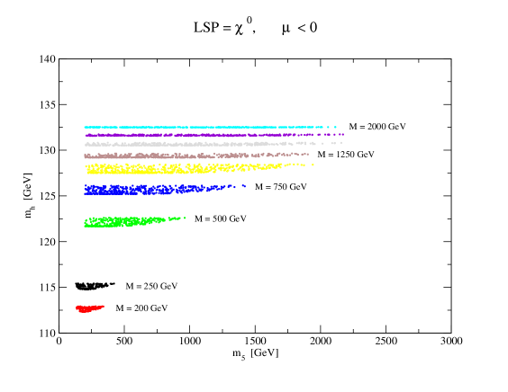
Figure 1: $m_{h}$ as function of $m_{\bf 5}$ for different values of $M$ for model $\bf FUTA$, for $\mu<0$.

In the SSB sector, besides the constraints imposed by finiteness there are further restrictions imposed by phenomenology. In the case where all the soft scalar masses are universal at the unfication scale, there is no region of $M$ below $O(few~{}TeV)$ in which $m_{\tilde{\tau}}>m_{\chi^{0}}$ is satisfied (where $m_{\tilde{\tau}}$ is the lightest $\tilde{\tau}$ mass, and $m_{\chi^{0}}$ the lightest neutralino mass, which is the lightest supersymmetric particle). But once the universality condition is relaxed this problem can be solved naturally (thanks to the sum rule). More specifically, using the sum rule (9) and imposing the conditions a) successful radiative electroweak symmetry breaking, b) $m_{\tilde{\tau}}^{2}>0$ and c) $m_{\tilde{\tau}}>m_{\chi^{0}}$, a comfortable parameter space for both models (although model ${\bf B}$ requires large $M\sim 1$ TeV) is found.

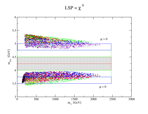
Figure 2: $m_{bot}(m_{bot})$ as function of $m_{\bf 5}$ for different values of $M$ for model $\bf FUTA$, for $\mu<0$ and $\mu>0$. The shaded region shows the experimentally accepted value of $m_{bot}(m_{bot})$ according to ref. [27].

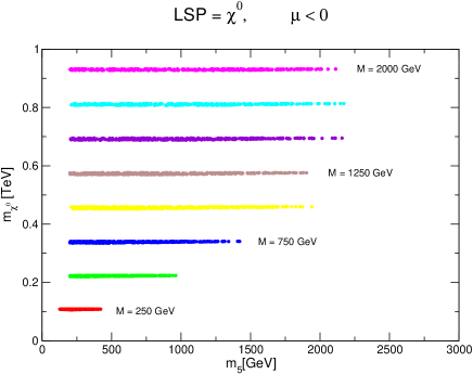
Figure 3: $m_{\chi^{0}}$ as function of $m_{\bf 5}$ for different values of $M$ for model $\bf FUTA$, for $\mu<0$.

As an additional constraint, we take into account the $BR(b\to s\gamma)$ [25]. We do not take into account, though, constraints coming from the muon anomalous magnetic moment (g-2) in this work, which excludes a small region of the parameter space. In the graphs we show the FUTA results concerning $m_{h}$, $m_{\chi^{0}}$, and $M_{A}$, for different values of $M$, for the case where $\mu<0$ and the LSP is a neutralino $\chi^{0}$. The results for $\mu>0$ are slightly different: the spectrum starts around 500 GeV. The main difference, though, is in the value of the running bottom mass $m_{bot}(m_{bot})$, where we have included the corrections coming from bottom squark-gluino loops and top squark-chargino loops [26]. In the $\mu<0$ case, $m_{bot}\sim 3.5-4.0~{}$ GeV is just below the experimental value $m_{bot}^{exp}\sim 4.0-4.5$ GeV [27], whereas in the $\mu>0$ case, $m_{bot}\sim 4.8-5.3$ GeV, i. e. above the experimental value.

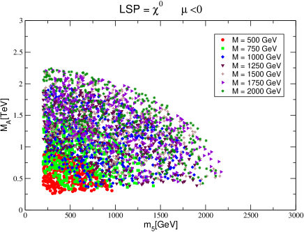
Figure 4: $M_{A}$ as function of $m_{\bf 5}$ for different values of $M$ for model $\bf FUTA$, for $\mu<0$.

$M_{top}$	183	$m_{bot}$	3.9
$\tan\beta=$	54.4	$\alpha_{s}$	.118
$m_{\chi_{1}}$	452	$m_{\tilde{\tau}_{2}}$	916
$m_{\chi_{2}}$	843	$m_{\tilde{\nu}_{3}}$	883
$m_{\chi_{3}}$	850	$\mu$	-1494
$m_{\chi_{4}}$	1500	$B$	3543
$m_{\chi^{\pm}_{1}}$	843	$m_{A}$	555
$m_{\chi^{\pm}_{2}}$	1500	$m_{H^{\pm}}$	560
$m_{\tilde{t}_{1}}$	1578	$m_{H}$	555
$m_{\tilde{t}_{2}}$	1776	$m_{h}$	127.5
$m_{\tilde{b}_{1}}$	1580	$M_{1}$	452
$m_{\tilde{b}_{2}}$	1766	$M_{2}$	846
$m_{\tilde{\tau}_{1}}$	654	$M_{3}$	2210

Table 1: A representative example of the bottom (running) and top (pole) masses, plus the supersymmetric spectrum for Model FUTA, with $m_{5}=$ 697 GeV, $m_{10}=$ 806 GeV, $M_{susy}=$ 1681 GeV, $\mu<0$. All masses in the Table are in GeV.

$M_{top}$	173	$m_{bot}$	4.2
$\tan\beta=$	48	$\alpha_{s}$	.116
$m_{\chi_{1}}$	669	$m_{\tilde{\tau}_{2}}$	970
$m_{\chi_{2}}$	912	$m_{\tilde{\nu}_{3}}$	916
$m_{\chi_{3}}$	1289	$\mu$	-1900
$m_{\chi_{4}}$	1909	$B$	4010
$m_{\chi^{\pm}_{1}}$	1289	$m_{A}$	1106
$m_{\chi^{\pm}_{2}}$	909	$m_{H^{\pm}}$	1109
$m_{\tilde{t}_{1}}$	2236	$m_{H}$	1106
$m_{\tilde{t}_{2}}$	2519	$m_{h}$	123.5
$m_{\tilde{b}_{1}}$	2163	$M_{1}$	700
$m_{\tilde{b}_{2}}$	2501	$M_{2}$	1293
$m_{\tilde{\tau}_{1}}$	766	$M_{3}$	3256

Table 2: A representative example of the bottom (running) and top (pole) masses, plus the supersymmetric spectrum for Model FUTB, with $m_{10}=$ 945 GeV, $M_{susy}=$ 2278 GeV, $\mu<0$. All masses in the Table are in GeV.

The Higgs mass prediction of the two models is, although the details of each of the models differ, in the following range

$$m_{h}=\quad\sim 112-132~{}~{}GeV,$$ (25)

where the uncertainty comes from variations of the gaugino mass $M$ and the soft scalar masses, and from finite (i.e. not logarithmically divergent) corrections in changing renormalization scheme. The one-loop radiative corrections have been included [28] for $m_{h}$, but not for the rest of the spectrum. In making the analysis, the value of $M$ was varied from $200-2000$ GeV for FUTA. We have also included a small variation, due to threshold corrections at the GUT scale, of $1-2\%$ of the FUT boundary conditions. This small variation does not give a noticeable effect in the results at low energies. From Fig. 1 we already see that the requirement $m_{h}>114.4$ GeV [29] (neglecting the theoretical uncertainties) excludes the possibility of $M=200$ GeV for FUTA, which is taken into account in the presentation of the next graphs. In Tables 1 and 2 we present representative examples of the values obtained for the s-spectra for each of the models.

A more detailed numerical analysis, where the results of our program and of the known programs FeynHiggs [30] and Suspect [31] are combined, is currently in progress [32].

References

- [1]
- [2] Kubo, J., Mondragón, M. and Zoupanos, G. (1994) Nucl. Phys. B424 291.
- [3] Zimmermann, W., (1985) Com. Math. Phys. 97 211; Oehme, R. and Zimmermann, W. (1985) Com. Math. Phys. 97 569; Ma,E. (1978) Phys.Rev D 17 623;ibid (1985) D31 1143.
- [4] Lucchesi, C., Piguet, O. and Sibold, K. (1988) Helv. Phys. Acta 61 321; Piguet, O. and Sibold, K. (1986) Intr. J. Mod. Phys. A1 913; (1986) Phys. Lett. B177 373; see also Lucchesi, C. and Zoupanos, G. (1997) Fortsch. Phys. 45 129.
- [5] Ermushev, A.Z., Kazakov, D.I. and Tarasov, O.V. (1987) Nucl. Phys. 281 72; Kazakov, D.I. (1987) Mod. Phys. Lett. A9 663.
- [6] Kapetanakis D., Mondragón, M. and Zoupanos, G., (1993) Zeit. f. Phys. C60 181; Mondragón, M. and Zoupanos, G. (1995) Nucl. Phys. B (Proc. Suppl.) 37C) 98.
- [7] Jack, I. and Jones, D.R.T. (1995) Phys. Lett. B349 294.
- [8] Kubo, J., Mondragón, M. and Zoupanos, G. (1996) Phys. Lett. B389 523.
- [9] D.R.T. Jones, L. Mezincescu and Y.-P. Yao, Phys. Lett. B148 317 (1984).
- [10] Jack, I. and Jones, D.R.T. (1994) Phys. Lett. B333 372.
- [11] Leigh, R.G., and Strassler, M.J. (1995) Nucl. Phys. B447 95.
- [12] Novikov, V., Shifman, M., Vainstein, A., and Zakharov, V. (1983) Nucl. Phys.B229 381; (1986)Phys. Lett. B166 329; Shifman, M. (1996) Int.J. Mod. Phys.A11 5761 and references therein.
- [13] Avdeev, L.V., Kazakov, D.I. and Kondrashuk, I.N. (1998) Nucl. Phys. B510 289; Kazakov, D.I. (1999) Phys.Lett. B449 201.
- [14] T. Kobayashi, J. Kubo and G. Zoupanos, (1998) Phys. Lett. B427 291; T. Kobayashi et al, in proc. of “Supersymmetry, Supergravity and Superstrings”, pp. 242-268, Seoul, 1999; T.Kobayashi et. al (2001) Surveys High Energy Phys. 16 87-129.
- [15] Yamada, Y. (1994) Phys.Rev. D50 3537.
- [16] J. Hisano and M. Shifman, Phys. Rev. D56 (1997) 5475.
- [17] Kawamura, T., Kobayashi, T. and Kubo, J. (1997) Phys. Lett. B405 64.
- [18] Delbourgo, R. (1975) Nuovo Cim 25A 646; Salam, A. and Strathdee, J. (1975) Nucl. Phys. B86 142; Fujikawa, K. and Lang, W. (1975) Nucl. Phys. B88 61; Grisaru, M.T., Rocek, M. and Siegel, W. (1979) Nucl. Phys. B59 429.
- [19] Girardello, L. and Grisaru, M.T. (1982) Nucl. Phys. B194 65; Helayel-Neto, J.A. (1984) Phys. Lett. B135 78; Feruglio, F., Helayel-Neto, J.A. and Legovini, F. (1985) Nucl. Phys. B249 533; Scholl, M. (1985) Zeit. f. Phys. C28 545.
- [20] I. Jack, D.R.T. Jones and A. Pickering, Phys. Lett. B426 (1998) 73.
- [21] Kobayashi, T., Kubo, J., Mondragón, M. and Zoupanos, G. (1998) Nucl. Phys. B511 45; in proc. of ICHEP 1998, vol. 2, p. 1597 (Vancouver 1998); Acta Phys. Polon. B30 (1999) 2013; in proc. of HEP99, p. 804 (Tampere 1999); M. Mondragon and G. Zoupanos, Acta Phys. Polon. B 34 (2003) 5459.
- [22] K. S. Babu, T. Enkhbat and I. Gogoladze (2003) Phys. Lett. B 555 238 [arXiv:hep-ph/0204246];
- [23] J. Erler, to appear in the next edition of the PDG, private communication.
- [24] For an extended discussion and a complete list of references see: Kubo, J., Mondragón, M. and Zoupanos, G. (1997) Acta Phys. Polon. B27 3911.
- [25] P. Cho, M. Misiak and D. Wyler, Phys. Rev. D 54, 3329 (1996); A. Kagan and M. Neubert, Eur. Phys. J. C 7 (1999) 5, K. Chetyrkin, M. Misiak and M. Munz, Phys. Lett. B 400, (1997) 206, [Erratum-ibid. B 425 (1998) 414] P. Gambino and M. Misiak, Nucl. Phys. B 611 (2001) 338, R. Barate et al. [ALEPH Collaboration], Phys. Lett. B 429 (1998) 169; S. Chen et al. [CLEO Collaboration], Phys. Rev. Lett. 87 (2001) 251807, K. Abe et al. [Belle Collaboration], Phys. Lett. B 511 (2001) 151, B. Aubert et al. [BABAR Collaboration];
- [26] L. J. Hall, R. Rattazzi and U. Sarid, Phys. Rev. D 50, (1994) 7048 [arXiv:hep-ph/9306309]; R. Hempfling, Z. Phys. C 63, (1994) 309 [arXiv:hep-ph/9404226]; F. M. Borzumati, M. Olechowski and S. Pokorski, Phys. Lett. B 349, (1995) 311 [arXiv:hep-ph/9412379]; T. Blazek, S. Raby and S. Pokorski, Phys. Rev. D 52, (1995) 4151 [arXiv:hep-ph/9504364]. M. Carena, M. Olechowski, S. Pokorski and C. E. M. Wagner, Nucl. Phys. B 426 (1994) 269 [arXiv:hep-ph/9402253].
- [27] K. Hagiwara et al., Phys. Rev. D66, 010001 (2002).
- [28] Gladyshev, A.V., Kazakov, D.I., de Boer, W., Burkart, G. and Ehret, R. (1997) Nucl. Phys. B498 3; Carena, M. et. al., (1995) Phys. Lett. B355 209.
- [29] LEP Higgs working group, Phys. Lett. B 565 (2003) 61, hep-ex/0306033.
- [30] S. Heinemeyer, W. Hollik and G. Weiglein, Comput. Phys. Commun. 124 (2000) 76 [arXiv:hep-ph/9812320]; ibid Eur. Phys. J. C 9 (1999) 343 [arXiv:hep-ph/9812472].
- [31] A. Djouadi, J. L. Kneur and G. Moultaka, arXiv:hep-ph/0211331.
- [32] Djouadi, A., Heinemeyer, S., Mondragón, M. and Zoupanos, G., work in progress.