$\pi K$ Scattering in Three Flavour ChPT

Abstract:

We present the scattering lengths for the $\pi K$ processes in the three flavour Chiral Perturbation Theory (ChPT) framework at next-to-next-to-leading order (NNLO). The calculation has been performed analytically but we only include analytical results for the dependence on the low-energy constants (LECs) at NNLO due to the size of the expressions. These results, together with resonance estimates of the NNLO LECs are used to obtain constraints on the Zweig rule suppressed LECs at NLO, $L_{4}^{r}$ and $L_{6}^{r}$. Contrary to expectations from NLO order calculations we find them to be compatible with zero. We do a preliminary study of combining the results from $\pi\pi$ scattering, $\pi K$ scattering and the scalar form-factors and find only a marginal compatibility with all experimental/dispersive input data.

1 Introduction

Effective Lagrangians have become a widely used tool in understanding physics involving a mass gap in the spectrum. They can be used in theories in a weakly coupled regime but with unknown underlying physics (as is the case in the Higgs sector of the standard model) or in theories with a strongly coupled regime where the usual perturbation formalism breaks down. Our interest will be focused on Quantum Chromo Dynamics (QCD). It is a well established theory at high energy where our theoretical knowledge and the experimental outcome agree with rather good accuracy. At low energy the situation is less satisfactory because the theory becomes strongly coupled and non-perturbative, standard perturbative methods can not be applied. One of the immediate differences is given by the degrees of freedom at low and high energy. At the former they are characterised by hadrons while in the latter they are better described in terms of the fundamental interacting quarks and gluons.

A suitable method to tackle phenomenology at low energy in the mesonic sector, besides direct numerical computation as done in lattice QCD, is to use the fact that QCD possesses an almost exact symmetry. One can then rely on these symmetries and their breaking pattern using an effective Lagrangian method. We will use the chiral symmetry present in the QCD Lagrangian in the limit of massless quarks. The use of this symmetry and the effective Lagrangian method is now known as Chiral Perturbation Theory (ChPT). It was introduced by Weinberg [1] and systematized by Gasser and Leutwyler [2] for the case of the light up and down quarks as well as for the case where the strange quark is treated as light in addition [3]. They performed a basic set of next-to-leading order (NLO) calculations allowing a first determination of all low-energy constants at NLO, the $L_{i}^{r}$, invoking the Zweig rule to set $L_{4}^{r}=L_{6}^{r}\approx 0$. It was hoped this could be tested in $K_{\ell 4}$ easily, but it turned out, when the explicit calculations were performed, that these only had very suppressed contributions to the form-factors [4, 5].

One question is how to order the various terms in the chiral expansions. The proposal used by most people is to count energies and momenta as a small parameter of order $p$ and the quark masses as order $p^{2}$. Alternative countings, taking the quark masses also as order $p$ are possible, see [6] and references therein. Combining the two-flavour two-loop calculations of $\pi\pi$ scattering [7, 8] and the pion scalar form-factor [9] with the Roy equation analysis [10] it could be shown that in the two flavour case the correct counting was the standard one [11, 12] using the recent determination of the pion scattering length from $K_{\ell 4}$ [13, 14].

The up and down quark masses are much smaller than the strange quark mass. The question thus remains whether three flavour ChPT itself converges sufficiently well to be of practical use and whether alternative countings of contributions involving the strange quark mass need to be used. This possibility is discussed in the recent work [15, 16]. The argument is that disconnected loop contributions from strange quarks, via kaons and etas, can be large, making a convergent three flavour ChPT difficult to achieve in the usual sense [16, 17]. Answering this question is part of the larger problem of whether the strange quark can be considered a light quark. This was part of the motivation behind the recent work in three flavour ChPT at NNLO on $\pi\pi$ scattering [18] and the various scalar form-factors [19]. Earlier calculations of the pseudoscalar masses and decay constants, see Ref. [20] and references therein, showed the possibility of this behaviour. The various vector form-factors calculated did not seem to have problems with convergence [21, 22, 23, 24].

Work on $\pi K$ scattering began soon after Weinberg’s calculation of $\pi\pi$ scattering [25]. The earliest reference known to us is [26]. During the 1970s there was a dedicated series of experiments culminating in the review by Lang [27]. These were used extensively together with dispersion relations and crossing symmetry in [28] and [29].

The development of ChPT led after some time to the calculation of the $\pi K$ scattering amplitude to NLO [30, 31]. There were also earlier attempts at unitarization of current algebra for this process. An example can be found in the discussion in [32, 33] and references therein. Other recent related works are the various attempts at putting in resonances in this process starting with [34]. Approaches involving resummations can be found in [35] and [36]. An alternative approach is to consider the kaon as heavy and treat only the pion as a Goldstone boson. This is known as heavy kaon ChPT. The applications to $\pi K$ scattering can be found in [37] and [38]. Unfortunately this approach has many free parameters and does not allow to connect $\pi K$ scattering to other processes. It does, however, have the possibility of being applicable even if standard ChPT does not work.

On the dispersive side, the analyses of [28] were slowly updated to get at a determination of the $p^{4}$ LECs. The first work was [39] and the full analysis has recently become available [40]. In the mean time, the isospin breaking corrections to $\pi K$ scattering at NLO have been evaluated in [41, 42, 43, 44]. Since we work in the isospin limit and the dispersive calculation of [40] has been performed in the same approximation we do not discuss these works further.

In this paper we calculate the standard ChPT expression for $\pi K$ scattering to next-to-next-to-leading-order. A large number of calculations to this order exist in three flavour ChPT and we have thus been able to determine most $p^{4}$ LECs with this precision after making some assumptions on the values of the $p^{6}$ constants. In earlier work it has been found that the Zweig rule suppressed constants $L_{4}^{r}$ and $L_{6}^{r}$ could be sufficiently different from zero that the scenario of large corrections due to disconnected strange quark loops was not ruled out. Pushing this calculation to NNLO allows then to perform this comparison at the same footing as all the other $p^{4}$ LECs. Earlier attempts at using $K_{\ell 4}$ had led to rather large errors for these constants, e.g. $L_{4}^{r}=(-0.2\pm 0.9)\,10^{-3}$[45]. The work on $\pi\pi$ scattering [18] and scalar form-factors [19] at NNLO order gave an indication that the region with $L_{4}^{r}\approx 0.45\,10^{-3}$ was preferred. This fitted with the NLO $\pi K$ work done earlier [40]. As discussed below, contrary to our expectations, the results from $\pi K$ scattering at NNLO are more indicative of a smaller value for $L_{4}^{r}$.

This paper is organized as follows. In Sect. 2 we give a very short overview of ChPT and the references for NNLO techniques. In Sect. 3 we discuss a few general properties of the $\pi K$ scattering amplitude. Sect. 4 gives an overview of our main result, the calculation of the $\pi K$ scattering amplitude to NNLO in three flavour ChPT. We also present here some plots showing the importance of the various contributions. The inputs we use to do the numerical analysis are described in Sect. 7. The main numerical analysis is presented in Sect. 8 and we give our conclusions in Sect. 9.

2 Chiral Perturbation Theory

ChPT is the effective field theory for QCD at low energies introduced in [1, 2, 3]. Introductory references are in Ref. [46]. The usual expansion is in quark masses and meson momenta generically labeled $p$ and assumes $m_{q}\sim p^{2}$. The Lagrangian for the strong and semi leptonic mesonic sector to NNLO can be written as

$${\cal L}={\cal L}_{2}+{\cal L}_{4}+{\cal L}_{6}\,,$$ (1)

where the subscript refers to the chiral order. The lowest order Lagrangian is

$${\cal L}_{2}=\frac{F_{0}^{2}}{4}\langle u_{\mu}u^{\mu}+\chi_{+}\rangle\,.$$ (2)

The mesonic fields enter in a non-linear fashion via $u=\exp\left(iM/(F_{0}\sqrt{2})\right)$, with $M$ parametrising the pseudoscalar fields. The quantity $u_{\mu}$ also contains the external vector ($v_{\mu}$) and axial-vector ($a_{\mu}$) currents

$$u_{\mu}=i(u^{\dagger}\partial_{\mu}u-\partial_{\mu}uu^{\dagger}-iu^{\dagger}r_{\mu}u+iul_{\mu}u^{\dagger})\,,\quad l_{\mu}(r_{\mu})=v_{\mu}-(+)a_{\mu}\,.$$ (3)

The scalar ($s$) and pseudo scalar ($p$) currents are contained in

$$\chi_{\pm}=u^{\dagger}\chi u^{\dagger}\pm u\chi^{\dagger}u\,,\quad\chi=2B_{0}\left(s+ip\right)\,.$$ (4)

The $p^{4}$ or NLO Lagrangian, ${\cal L}_{4}$, was introduced in Ref. [3] and is of the general form

$${\cal L}_{4}=\sum_{i=1}^{12}L_{i}P_{i}=\ldots+L_{4}\langle u^{\mu}u_{\mu}\rangle\langle\chi_{+}\rangle+L_{6}\langle\chi_{+}\rangle^{2}+\ldots\,.$$

We have explicitly shown two terms with chiral symmetry breaking which in addition present a double flavour trace structure, which indicates that these two terms are suppressed by the Zweig rule.

The schematic form of the NNLO Lagrangian in the three flavour case is

$${\cal L}_{6}=\sum_{i=1,94}C_{i}\,O_{i}$$ (5)

and we refer to [47] for their explicit expressions.

The ultra-violet divergences produced by loop diagrams of order $p^{4}$ and $p^{6}$ cancel in the process of renormalization with the divergences extracted from the low-energy constants $L_{i}$’s and $C_{i}$’s. We use dimensional regularization and the modified minimal subtraction $(\overline{MS})$ version usually used in ChPT. An extensive description of the regularization and renormalization procedure can be found in Refs. [8] and [48]. The divergences are known in general [48, 2, 3, 49] and their cancellation is a check on our calculation.

3 The $\pi K$ amplitude: general properties

The $\pi K$ scattering amplitude in isospin channel $I$ can be written as

$$A(\left(\pi(p_{1})K(p_{2})\to\pi(p_{3})K(p_{4})\right)=T^{I}(s,t,u)\,.$$ (6)

$s,t,u$ are the usual Mandelstam variables

$$s=(p_{1}+p_{2})^{2}\,,\quad t=(p_{1}-p_{3})^{2}\quad\mbox{and}\quad u=(p_{1}-p_{4})^{2}\,.$$ (7)

There are two possible isospin combinations $I=1/2$ and $I=3/2$. These two are related via $s\leftrightarrow u$ crossing which yields

$$T^{\frac{1}{2}}(s,t,u)=-\frac{1}{2}T^{\frac{3}{2}}(s,t,u)+\frac{3}{2}T^{\frac{3}{2}}(u,t,s)\,.$$ (8)

We also define the crossing symmetric amplitudes $T^{+}$ and $T^{-}$ as,

$$T^{\pm}(s,t,u)=\frac{1}{2}\left(\pm T^{\frac{3}{2}}(s,t,u)+T^{\frac{3}{2}}(u,t,s)\right)\,.$$ (9)

These amplitudes can be calculated most easily from the purely $I=3/2$ process $\pi^{+}K^{+}\to\pi^{+}K^{+}$.

In order to describe scattering kinematics it is convenient to introduce the variable

$$q_{\pi K}^{2}=\frac{s}{4}\left(1-\frac{(m_{K}+m_{\pi})^{2}}{s}\right)\left(1-\frac{(m_{K}-m_{\pi})^{2}}{s}\right)\,.$$ (10)

The kinematical variables $t,u$ can be expressed in terms of $s$ and $\cos\theta$ as

$$t=-2q_{\pi K}^{2}(1-\cos\theta)\,,\quad u=-s-t+2m_{K}^{2}+2m_{\pi}^{2}\,.$$ (11)

The various amplitudes are expanded in partial waves via

$$T^{I}(s,t,u)=16\pi\sum_{\ell=0}^{\infty}(2\ell+1)P_{\ell}(\cos\theta)t^{I}_{\ell}(s)\,.$$ (12)

Near threshold these can be expanded in a Taylor series

$$t^{I}_{\ell}(s)\equiv\frac{1}{2}\sqrt{s}q_{\pi K}^{2\ell}\left(a^{I}_{\ell}+b^{I}_{\ell}q_{\pi K}^{2}+{\cal O}(q_{\pi K}^{4})\right)\,,$$ (13)

defining the threshold parameters $a^{I}_{\ell}$ and $b^{I}_{\ell}$.

Below the inelastic threshold the partial waves satisfy

$$\mbox{Im}t^{I}_{\ell}(s)=\frac{2q_{\pi K}}{\sqrt{s}}\left|t^{I}_{\ell}(s)\right|^{2}\,.$$ (14)

In ChPT the inelasticity only starts at order $p^{8}$. In this regime the partial waves can be written in terms of the phase-shifts as

$$t^{I}_{\ell}(s)=\frac{\sqrt{s}}{2q_{\pi K}}\,\frac{1}{2i}\left\{e^{2i\delta^{I}_{\ell}(s)}-1\right\}\,.$$ (15)

The amplitudes are often expanded around the point $t=0$, $s=u$ via

$$T^{+}(s,t,u) = \sum_{i,j=0}^{\infty}c^{+}_{ij}t^{j}\nu^{2j}\,,$$

$$T^{-}(s,t,u) = \sum_{i,j=0}^{\infty}c^{-}_{ij}t^{j}\nu^{2j+1}\,,$$ (16)

where $\nu=(s-u)/(4m_{K})$ and the $c^{\pm}_{ij}$ are referred to as subthreshold expansion parameters. They are normally quoted in units of the relevant power of $m_{\pi^{+}}$. We will always list these parameters in increasing order corresponding to powers of $t$ and $s-u$.

The $p^{2}$ result for the amplitude has only a few nonzero items. As a consequence the imaginary parts for all other partial waves starts only at order $p^{8}$. This allows the amplitude to be written in the form

$$T^{\frac{3}{2}}(s,t,u)=G_{1}(s)+G_{2}(t)+G_{3}(u)+(s-u)G_{4}(t)+(s-t)G_{5}(u)\,.$$ (17)

The functions $G_{i}(s)$ have a polynomial ambiguity due to $s+t+u=2m_{\pi}^{2}+2m_{K}^{2}$. The functions $G_{i}(s)$ have various singularities. $G_{1}$, $G_{3}$ and $G_{5}$ contain singularities from the $\pi K$ and $\eta K$ intermediate states and $G_{2}$ and $G_{4}$ from the possible nonstrange two meson intermediates. The precise relation with the various singularities can be found in [39].

4 ChPT results

4.1 Results at order $p^{2}$

The lowest order result is very simple and corresponds to

$$c^{+}_{00}=0,\quad c^{+}_{10}=\frac{1}{4F_{\pi}^{2}}\quad\mbox{and}\quad c^{-}_{00}=\frac{m_{K}}{F_{\pi}^{2}}\,.$$ (18)

All higher terms vanish. This was initially performed using current algebra methods [26].

4.2 Results at order $p^{4}$

The next-to-leading calculation was first performed in [30, 31]. We present it here in a slightly different form, but the final expression given in that reference agrees with ours up to terms of order $p^{6}$. Note that as mentioned also in [39] there are some misprints in the formulas in [30].

We present the analytical expressions for the $G_{i}$ functions defined in (17) and where the polynomial part was isolated in a function $G_{6}(s,t,u)$. We also use $\Delta=m_{K}^{2}-m_{\pi}^{2}$ and $\Sigma=m_{K}^{2}+m_{\pi}^{2}$.

$$F_{\pi}^{4}\,G_{1}(s) = \overline{B}(m_{\pi}^{2},m_{K}^{2},s)\,(-1/2\,s\,\Sigma+1/4\,s^{2}+1/4\Sigma^{2})\,,$$ (19)

$$F_{\pi}^{4}\,G_{2}(t) = \overline{B}(m_{\pi}^{2},m_{\pi}^{2},t)\,(1/16\,t\,\Delta-1/16\,t\,\Sigma+1/4\,t^{2})$$ (20)

$$+\overline{B}(m_{K}^{2},m_{K}^{2},t)\,(3/16\,t^{2})$$

$$+\overline{B}(m_{\eta}^{2},m_{\eta}^{2},t)\,(1/24\,m_{\eta}^{2}\,\Delta-1/24\,m_{\eta}^{2}\,\Sigma-1/16\,t\,\Delta$$

$$\hskip 28.45274pt+1/16\,t\,\Sigma+1/72\,\Delta\,\Sigma-1/144\,\Delta^{2}-1/144\,\Sigma^{2})\,,$$

$$F_{\pi}^{4}G_{3}(u) = \overline{B}(m_{\pi}^{2},m_{K}^{2},u)\,(-3/8\,u\,\Sigma+11/32\,u^{2}+1/8\Delta\Sigma$$ (21)

$$\hskip 85.35826pt-7/32\Delta^{2}+1/8\Sigma^{2})$$

$$+\overline{B}(m_{K}^{2},m_{\eta}^{2},u)\,(-1/16\,m_{\eta}^{2}\,u-41/288\,m_{\eta}^{2}\,\Delta+1/32\,m_{\eta}^{2}\,\Sigma$$

$$\hskip 85.35826pt+1/96\,m_{\eta}^{4}+5/96\,u\,\Delta-3/32\,u\,\Sigma+3/32\,u^{2}$$

$$\hskip 85.35826pt+31/192\,\Delta\,\Sigma+493/3456\,\Delta^{2}+3/128\,\Sigma^{2})$$

$$+\overline{B}_{1}(m_{\pi}^{2},m_{K}^{2},u)\,(-1/4\Delta\Sigma-3/8\Delta^{2})$$

$$+\overline{B}_{1}(m_{K}^{2},m_{\eta}^{2},u)\,(-1/8\,m_{\eta}^{2}\,\Delta-3/16\,\Delta\,\Sigma-13/48\,\Delta^{2})$$

$$+\overline{B}_{21}(m_{\pi}^{2},m_{K}^{2},u)\,(3/8\Delta^{2})$$

$$+\overline{B}_{21}(m_{K}^{2},m_{\eta}^{2},u)\,(3/8\Delta^{2})\,,$$

$$F_{\pi}^{4}\,G_{4}(t) = \overline{B}(m_{\pi}^{2},m_{\pi}^{2},t)\,(-1/24\,t\,-1/12\Delta+1/12\Sigma)$$ (22)

$$+\overline{B}(m_{K}^{2},m_{K}^{2},t)\,(-1/48\,t\,+1/24\Delta+1/24\Sigma)\,,$$

$$F_{\pi}^{4}\,G_{5}(u) = \overline{B}(m_{\pi}^{2},m_{K}^{2},u)\,(-1/32u-1/32\Delta+1/16\Sigma)$$ (23)

$$+\overline{B}(m_{K}^{2},m_{\eta}^{2},u)\,(1/32\,m_{\eta}^{2}-1/32\,u+3/64\,\Delta+3/64\,\Sigma)$$

$$+\overline{B}_{1}(m_{\pi}^{2},m_{K}^{2},u)\,(1/16\Delta)$$

$$+\overline{B}_{1}(m_{K}^{2},m_{\eta}^{2},u)\,(1/16\,m_{\eta}^{2}-1/32\,\Delta-1/32\,\Sigma)\,,$$

$$F_{\pi}^{4}\,G_{6}(s,t,u) = F_{\pi}^{2}(-1/2\,s\,+1/2\Sigma)$$

$$+(16\pi^{2})^{-1}\,(3/32\,m_{\eta}^{2}\,s-1/32\,m_{\eta}^{2}\,(t-u)-1/16\,m_{\eta}^{2}\,\Sigma$$

$$\hskip 56.9055pt-1/64\,s\,\Delta+31/192\,s\,\Sigma+1/16\,s^{2}-7/192\,(t-u)\,\Delta$$

$$\hskip 56.9055pt+1/64\,(t-u)\,\Sigma-1/48\,(t-u)^{2}+1/96\,\Delta\,\Sigma-13/96\,\Sigma^{2})$$

$$+L_{1}^{r}\,\,(-4\,s\,(t-u)+2\,s^{2}+2(t-u)^{2}-8\Delta^{2})$$

$$+L_{2}^{r}\,\,(2\,s\,(t-u)-8\,s\,\Sigma+5\,s^{2}+(t-u)^{2}+4\Sigma^{2})$$

$$+L_{3}^{r}\,\,(\,s^{2}+(t-u)^{2}-2\Delta^{2})$$

$$+L_{4}^{r}\,\,(-4\,s\,\Sigma+4(t-u)\Sigma+8\Delta^{2})$$

$$+L_{5}^{r}\,\,(2\,s\,\Delta-2\,s\,\Sigma-2\Delta\Sigma+2\Delta^{2})$$

$$+L_{6}^{r}\,\,(-8\Delta^{2}+8\Sigma^{2})$$

$$+L_{8}^{r}\,\,(-4\Delta^{2}+4\Sigma^{2})$$

$$+\overline{A}(m_{\pi}^{2})\,-21/32\,s-5/96\,(t-u)-7/32\,\Delta+13/24\,\Sigma)$$

$$+\overline{A}(m_{K}^{2})\,(1/96\,m_{\eta}^{2}-3/16\,s+1/48\,(t-u)+31/576\,\Delta+5/64\,\Sigma)$$

$$+\overline{A}(m_{\eta}^{2})\,(9/160\,m_{\eta}^{2}+3/32\,s+1/32\,(t-u)+7/64\,\Delta-49/320\,\Sigma)\,.$$

The finite part of the one-loop integrals are denoted by $\overline{A},\overline{B}_{j}$ as defined in [20].

4.3 Results at order $p^{6}$

The full result at order $p^{6}$ is rather cumbersome. In this section we quote only the dependence on the order $p^{6}$ constants. This contribution can be written exactly in the form of the subthreshold expansion (3) with as nonzero combinations, normalized to $F_{\pi}^{4}\,m_{\pi^{+}}^{2i+2j}$ and $F_{\pi}^{4}\,m_{\pi^{+}}^{2i+2j+1}$ for $c^{+}_{ij}$ and $c^{-}_{ij}$ respectively,

$$c^{+}_{00} = 16\,m_{K^{+}}^{2}\,m_{\pi^{+}}^{4}\,(C^{r}_{1}+4\,C^{r}_{2}+C^{r}_{5}+C^{r}_{6}+2\,C^{r}_{7}-C^{r}_{12}-4\,C^{r}_{13}-2\,C^{r}_{14}-3\,C^{r}_{15}$$

$$\qquad\qquad\qquad-4\,C^{r}_{16}+3\,C^{r}_{19}+6\,C^{r}_{20}+12\,C^{r}_{21}-C^{r}_{26}-4\,C^{r}_{28}+3\,C^{r}_{31}+6\,C^{r}_{32})$$

$$+16\,m_{K^{+}}^{4}\,m_{\pi^{+}}^{2}\,(C^{r}_{1}+4\,C^{r}_{2}+2\,C^{r}_{6}+2\,C^{r}_{7}+C^{r}_{8}-C^{r}_{12}-4\,C^{r}_{13}-4\,C^{r}_{15}-4\,C^{r}_{16}$$

$$\qquad\qquad\qquad-2\,C^{r}_{17}+3\,C^{r}_{19}+8\,C^{r}_{20}+24\,C^{r}_{21}-C^{r}_{26}-4\,C^{r}_{28}+3\,C^{r}_{31}+8\,C^{r}_{32})\,,$$

$$c^{+}_{10} = 8\,m_{K^{+}}^{2}\,m_{\pi^{+}}^{2}\,(-4\,C^{r}_{1}-16\,C^{r}_{2}+2\,C^{r}_{4}-C^{r}_{5}-3\,C^{r}_{6}-4\,C^{r}_{7}-C^{r}_{8}+4\,C^{r}_{12}+10\,C^{r}_{13}$$

$$\qquad\qquad\qquad+C^{r}_{14}+5\,C^{r}_{15}+2\,C^{r}_{17}-2\,C^{r}_{22}-2\,C^{r}_{25}-C^{r}_{26}-2\,C^{r}_{29}-4\,C^{r}_{30})$$

$$+8\,m_{K^{+}}^{4}\,(-C^{r}_{1}-4\,C^{r}_{2}-2\,C^{r}_{6}-2\,C^{r}_{7}-C^{r}_{8}-2\,C^{r}_{12}-4\,C^{r}_{13}$$

$$\qquad\qquad-C^{r}_{14}+4\,C^{r}_{16}+C^{r}_{26}+4\,C^{r}_{28})$$

$$+8\,m_{\pi^{+}}^{4}\,(-C^{r}_{1}-4\,C^{r}_{2}-C^{r}_{5}-C^{r}_{6}-2\,C^{r}_{7}-2\,C^{r}_{12}$$

$$\qquad\qquad-2\,C^{r}_{13}+C^{r}_{14}+1/2\,C^{r}_{15}+4\,C^{r}_{16}-C^{r}_{17}+C^{r}_{26}+4\,C^{r}_{28})\,,$$

$$c^{-}_{00} = 16\,m_{K^{+}}\,m_{\pi^{+}}^{4}\,(C^{r}_{15}+2\,C^{r}_{17})$$

$$+16\,m_{K^{+}}^{3}\,m_{\pi^{+}}^{3}\,(4\,C^{r}_{4}+2\,C^{r}_{14}+2\,C^{r}_{15}-4\,C^{r}_{22}+4\,C^{r}_{25}+2\,C^{r}_{26}-4\,C^{r}_{29})\,,$$

$$c^{+}_{20} = m_{K^{+}}^{2}\,(12\,C^{r}_{1}+48\,C^{r}_{2}-8\,C^{r}_{4}+C^{r}_{5}+10\,C^{r}_{6}+8\,C^{r}_{7}+4\,C^{r}_{8}+C^{r}_{10}$$

$$\qquad\qquad+4\,C^{r}_{11}-2\,C^{r}_{12}-4\,C^{r}_{13}+2\,C^{r}_{22}-4\,C^{r}_{23}+4\,C^{r}_{25})$$

$$+m_{\pi^{+}}^{2}\,(12\,C^{r}_{1}+48\,C^{r}_{2}-8\,C^{r}_{4}+4\,C^{r}_{5}+5\,C^{r}_{6}+8\,C^{r}_{7}+C^{r}_{8}+C^{r}_{10}$$

$$\qquad\qquad+2\,C^{r}_{11}-2\,C^{r}_{12}-10\,C^{r}_{13}+2\,C^{r}_{22}-4\,C^{r}_{23}+4\,C^{r}_{25})\,,$$

$$c^{-}_{10} = 8\,m_{K^{+}}\,m_{\pi^{+}}^{2}\,(-4\,C^{r}_{4}-C^{r}_{6}-C^{r}_{8}+C^{r}_{10}+2\,C^{r}_{11}-2\,C^{r}_{12}-6\,C^{r}_{13}+2\,C^{r}_{22}-2\,C^{r}_{25})$$

$$+8\,m_{K^{+}}^{3}\,m_{\pi^{+}}\,(-4\,C^{r}_{4}-C^{r}_{5}-2\,C^{r}_{6}+C^{r}_{10}+4\,C^{r}_{11}-2\,C^{r}_{12}-12\,C^{r}_{13}+2\,C^{r}_{22}$$

$$\qquad\qquad\qquad-2\,C^{r}_{25})\,,$$

$$c^{+}_{01} = 16\,m_{K^{+}}^{2}\,m_{\pi^{+}}^{2}\,(C^{r}_{6}+C^{r}_{8}+C^{r}_{10}+2\,C^{r}_{11}-2\,C^{r}_{12}-2\,C^{r}_{13}+2\,C^{r}_{22}+4\,C^{r}_{23})$$

$$+16\,m_{K^{+}}^{4}\,m_{\pi^{+}}^{2}\,(C^{r}_{5}+2\,C^{r}_{6}+C^{r}_{10}+4\,C^{r}_{11}-2\,C^{r}_{12}-4\,C^{r}_{13}+2\,C^{r}_{22}+4\,C^{r}_{23})\,,$$

$$c^{+}_{30} = 1/2\,(-7\,C^{r}_{1}-32\,C^{r}_{2}+2\,C^{r}_{3}+10\,C^{r}_{4})\,,$$

$$c^{-}_{20} = 6\,m_{K^{+}}\,(-C^{r}_{1}+2\,C^{r}_{3}+2\,C^{r}_{4})\,,$$

$$c^{+}_{11} = 8\,m_{K^{+}}^{2}\,(3\,C^{r}_{1}+6\,C^{r}_{3}-2\,C^{r}_{4})\,,$$

$$c^{-}_{01} = 32\,m_{K^{+}}^{3}\,(-C^{r}_{1}+2\,C^{r}_{3}+2\,C^{r}_{4})\,.$$ (25)

Notice that the combinations $(-C^{r}_{1}+2\,C^{r}_{3}+2\,C^{r}_{4})$ shows up in both $c^{-}_{20}$ and $c^{-}_{01}$.

5 Resonance estimate of the contribution from the $p^{6}$ constants

Up to now we relied only on chiral symmetries to calculate the amplitude function at low energy. In order to give an estimate of the $p^{6}$ LECs, we assume our process to be saturated by the exchange of vector and scalar meson resonances. The general formalism of resonance saturation (RS) in ChPT was described in [51], [52]. The places where comparisons with experiment are available are in general in reasonable agreement with the estimates obtained via RS.

For both types of exchange, we only consider the polynomial contributions to $K\pi$-scattering starting at $\mathcal{O}(p^{6})$, thus directly corresponding to the $C_{i}^{r}$’s LEC’s contribution.

The vector resonances are included through the matrix of fields $V^{\mu}$ [53] with Lagrangian

$${\cal L}_{V}=-\frac{1}{4}\langle V_{\mu\nu}V^{\mu\nu}\rangle+\frac{1}{2}m_{V}^{2}\langle V_{\mu}V^{\mu}\rangle-\frac{ig_{V}}{2\sqrt{2}}\langle V_{\mu\nu}[u^{\mu},u^{\nu}]\rangle+f_{\chi}\langle V_{\mu}[u^{\mu},\chi_{-}]\rangle$$ (26)

while for the scalar meson nonet, the matrix of fields $S$, we consider

$${\cal L}_{S}=\frac{1}{2}\langle\nabla^{\mu}S\nabla_{\mu}S-M^{2}_{S}S^{2}\rangle+c_{d}\langle Su^{\mu}u_{\mu}\rangle+c_{m}\langle S\chi_{+}\rangle$$ (27)

After integration of the resonance fields, the Lagrangians relevant to the present case read

$${\cal L}_{V}=-\frac{1}{4M^{2}_{V}}\left\langle\left(ig_{V}\,\nabla_{\mu}[u^{\nu},u^{\mu}]-f_{\chi}\sqrt{2}\,[u^{\nu},\chi_{-}]\right)^{2}\right\rangle$$ (28)

$${\cal L}_{S}=\frac{1}{2M^{4}_{S}}\left\langle\left(c_{d}\nabla^{\nu}(u_{\mu}u^{\mu})+c_{m}\nabla^{\nu}\chi_{+}\right)^{2}\right\rangle$$ (29)

where we use [8]

$$f_{\chi}=-0.025,\quad g_{V}=0.09,\quad c_{m}=42\mbox{ MeV},\quad c_{d}=32\mbox{ MeV},$$ (30)

and the masses are

$$m_{V}=m_{\rho}=0.77\mbox{ GeV}, m_{A}=m_{a_{1}}=1.23\mbox{ GeV}, m_{S}=0.98\mbox{ GeV}.$$ (31)

The numerical results from both contributions to the subthreshold expansion parameters are listed in Table 1. The contribution to the full amplitude at order $p^{6}$ corresponds precisely to the expansion (3) including only these subthreshold constants. The explicit expressions for the nonzero constants are

$$c^{+}_{00} = -16\,f_{\chi}\,g_{V}/(M_{V}^{2}\sqrt{2})\,(m_{K}^{2}\,m_{\pi}^{4}+m_{K}^{4}\,m_{\pi}^{2})+4\,c_{m}^{2}/M_{S}^{4}\,(m_{K}^{2}\,m_{\pi}^{4}+m_{K}^{4}\,m_{\pi}^{2})$$

$$-16\,f_{\chi}^{2}/M_{V}^{2}\,(m_{K}^{2}\,m_{\pi}^{4}+m_{K}^{4}\,m_{\pi}^{2})-2\,g_{V}^{2}/M_{V}^{2}\,(m_{K}^{2}\,m_{\pi}^{4}+m_{K}^{4}\,m_{\pi}^{2})\,,$$

$$c^{+}_{10} = 8\,f_{\chi}\,g_{V}/(M_{V}^{2}\sqrt{2})\,(2\,m_{K}^{2}\,m_{\pi}^{2}+\,m_{K}^{4}+\,m_{\pi}^{4})-c_{d}\,c_{m}/M_{S}^{4}\,(12\,m_{K}^{2}\,m_{\pi}^{2})$$

$$+c_{d}^{2}/M_{S}^{4}\,(4\,m_{K}^{2}\,m_{\pi}^{2})+2\,c_{m}^{2}/M_{S}^{4}\,(3\,m_{K}^{2}\,m_{\pi}^{2}-\,m_{K}^{4}-\,m_{\pi}^{4})$$

$$+8\,f_{\chi}^{2}/M_{V}^{2}\,(\,m_{K}^{2}\,m_{\pi}^{2}+\,m_{K}^{4}+\,m_{\pi}^{4})+g_{V}^{2}/M_{V}^{2}\,(3\,m_{K}^{2}\,m_{\pi}^{2}+m_{K}^{4}+m_{\pi}^{4})\,,$$

$$c^{-}_{00} = c_{d}\,c_{m}/M_{S}^{4}\,(16\,m_{K}^{3}\,m_{\pi}^{2})+c_{m}^{2}/M_{S}^{4}\,(8\,m_{K}^{3}\,m_{\pi}^{2})$$

$$+f_{\chi}^{2}/M_{V}^{2}\,(96\,m_{K}^{3}\,m_{\pi}^{2})-g_{V}^{2}/M_{V}^{2}\,(4\,m_{K}^{3}\,m_{\pi}^{2})\,,$$

$$c^{+}_{20} = -3\,f_{\chi}\,g_{V}/(M_{V}^{2}\sqrt{2})\,(\,m_{K}^{2}+\,m_{\pi}^{2})+5/2\,c_{d}\,c_{m}/M_{S}^{4}\,(m_{K}^{2}+m_{\pi}^{2})$$

$$-7/4\,c_{d}^{2}/M_{S}^{4}\,(m_{K}^{2}+m_{\pi}^{2})-7/8\,g_{V}^{2}/M_{V}^{2}\,(m_{K}^{2}+m_{\pi}^{2})\,,$$

$$c^{-}_{10} = 24\,f_{\chi}\,g_{V}/(M_{V}^{2}\sqrt{2})\,(m_{K}\,m_{\pi}^{2}+m_{K}^{3})-4\,c_{d}\,c_{m}/M_{S}^{4}\,(m_{K}\,m_{\pi}^{2}+m_{K}^{3})$$

$$-2\,c_{d}^{2}/M_{S}^{4}\,(m_{K}\,m_{\pi}^{2}+m_{K}^{3})+3\,g_{V}^{2}/M_{V}^{2}\,(m_{K}\,m_{\pi}^{2}+m_{K}^{3})\,,$$

$$c^{+}_{01} = 16\,f_{\chi}\,g_{V}/(M_{V}^{2}\sqrt{2})\,(m_{K}^{2}\,m_{\pi}^{2}+m_{K}^{4})+8\,c_{d}\,c_{m}/M_{S}^{4}\,(m_{K}^{2}\,m_{\pi}^{2}+m_{K}^{4})$$

$$+4\,c_{d}^{2}/M_{S}^{4}\,(m_{K}^{2}\,m_{\pi}^{2}+m_{K}^{4})+2\,g_{V}^{2}/M_{V}^{2}\,(m_{K}^{2}\,m_{\pi}^{2}+m_{K}^{4})\,,$$

$$c^{+}_{30} = c_{d}^{2}/M_{S}^{4}\,(7/8)+g_{V}^{2}/M_{V}^{2}\,(3/16)\,,$$

$$c^{-}_{20} = c_{d}^{2}/M_{S}^{4}\,(3/2\,m_{K})+g_{V}^{2}/M_{V}^{2}\,(3/4\,m_{K})\,,$$

$$c^{+}_{11} = -6\,c_{d}^{2}/M_{S}^{4}\,(m_{K}^{2})+g_{V}^{2}/M_{V}^{2}\,(m_{K}^{2})\,,$$

$$c^{-}_{01} = c_{d}^{2}/M_{S}^{4}\,(8\,m_{K}^{3})+g_{V}^{2}/M_{V}^{2}\,(4\,m_{K}^{3})\,.$$ (32)

	Vector	Scalar	Sum Reso	chiral order	$p^{2}$	$p^{4}$	$p^{6}$
$c^{+}_{00}$	$-$0.02	0.13	0.11	2	0	0.122	0.007
$c^{+}_{10}$	0.018	$-$0.063	$-$0.045	2	0.5704	$-$0.113	0.460
$c^{-}_{00}$	0.21	0.17	0.38	2	8.070	0.311	0.017
$c^{+}_{20}$	$-$0.0053	0.0023	$-$0.0030	4	—	0.0256	$-$0.0254
$c^{-}_{10}$	$-$0.11	$-$0.04	$-$0.15	4	—	$-$0.0254	0.121
$c^{+}_{01}$	$-$0.27	0.28	0.01	4	—	1.667	1.492
$c^{+}_{30}$	0.00026	0.00010	0.00036	6	—	0.00121	0.00071
$c^{-}_{20}$	0.0037	0.00060	0.0043	6	—	0.00478	0.00320
$c^{+}_{11}$	0.017	$-$0.008	0.009	6	—	$-$0.126	$-$0.006
$c^{-}_{01}$	0.25	0.04	0.29	6	—	0.229	0.196

Table 1: The resonance contributions to the subthreshold parameters. The units are $m_{\pi^{+}}^{2i+2j}$ and $m_{\pi^{+}}^{2i+2j+1}$ for $c^{+}_{ij}$ and $c^{-}_{ij}$ respectively. We have also shown the chiral order at which they first have tree level contributions as well as the contributions with the $L_{i}^{r}=C_{i}^{r}=0$ at $\mu=0.77$ GeV.

Even if many of our results only get a small contribution from the above RS arguments, these estimates are in general a major source of uncertainty in the $\mathcal{O}(p^{6})$ terms. The estimates from resonance exchange for the masses and decay constants and the related sigma terms are the most uncertain because of the simple treatment of the scalar sector. These are discussed in more detail in [20] and [54]. Here we have set many effects, e.g. the $d_{m}$ term of [20], equal to zero, the naive size estimate of [20] led to anomalously large NNLO corrections. The estimates of the $K_{\ell 4}$ amplitudes can be found in [53] after the work of [55]. The effect of varying these was studied in [53] and found to be reasonable.

The above procedure is obviously subtraction point dependent and is normally only performed to leading order in the expansion in $1/N_{c}$, with $N_{c}$ the number of colours. Many other approaches exist, some recent relevant papers addressing this issue are [54, 56, 57] and references therein. A systematic study of this issue is clearly important, for our present first study the estimates are sufficient.

6 A first numerical look

In this section we present a first look at the numerical results for the two loop amplitudes. We choose as input the pion decay constant, the charged pion mass, the charged kaon mass and the physical eta mass.

$$F_{\pi} = 92.4~{}\mbox{MeV}\,,\qquad m_{\pi}=m_{\pi^{+}}=139.56995~{}\mbox{MeV}\,,$$

$$m_{K} = m_{K^{+}}=493.677~{}\mbox{MeV}\,,\quad m_{\eta}=547.3~{}\mbox{MeV}\,.$$ (33)

The subtraction scale $\mu=770~{}\mbox{MeV}$ is used throughout the paper unless otherwise mentioned explicitly.

We present the results for the subthreshold parameters with all $L_{i}^{r}$ and $C_{i}^{r}$ set equal to zero at the scale of the rho mass. Notice that the very different sizes of the various quantities are to a large extent given by their normalization in powers of $m_{K}$ and $m_{\pi}$.

The order $p^{4}$ results differ somewhat from those quoted in [30] and [39]. The reason for this is that some variation in the choice of precisely what is called $p^{4}$ and $p^{6}$ is possible. The choice we have made is different from those in the mentioned papers. Especially $c^{+}_{00}$ suffers from this numerically. E.g. taking the eta mass given by the Gell-Mann-Okubo formula instead, the numerical $p^{4}$ result for it changes to $0.16$. We conclude that we are also in numerical agreement with those papers.

The higher order corrections look very large when looked upon as the contributions to the various terms in the expansions. This is partly due to cancellations making some quantities very sensitive to higher order corrections.

Figure 1: The corrections at order $p^{2}$, $p^{4}$ and $p^{6}$ to the $S$ partial wave in the $I=1/2$ channel with all LECs set to zero at $\mu=0.77$ GeV.

Figure 2: The corrections at order $p^{2}$, $p^{4}$ and $p^{6}$ to the $S$ partial wave in the $I=3/2$ channel with all LECs set to zero at $\mu=0.77$ GeV.

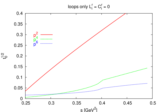
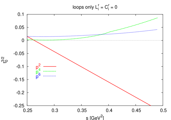
We also present some plots of the $S$ channel partial waves both in the $I=1/2$ and $I=3/2$ channel. These are shown in respectively Fig. 1 and Fig. 2. Two points of interest are $s=0.263$ GeV² for the subthreshold expansion and the threshold at $s=0.401$ GeV². From the sizes of the contributions at orders $p^{2}$, $p^{4}$ and $p^{6}$ as shown it is obvious that there seems to be a better convergence near threshold than at the subthreshold point. Contrary to the $\pi\pi$ scattering case, the lowest order result has already nonlinearities. The amplitude at this level is perfectly linear in $s$, $t$ and $u$ but in taking the partial waves, $t$ and $u$ depend nonlinearly on $s$ via $q^{2}_{\pi K}$. The partial waves have been extracted from the amplitudes using a five point Gaussian integration over $\cos\theta$.

	$p^{2}$	$p^{4}$	$p^{6}$	Reso
$a^{1/2}_{0}$	0.142	0.035	0.022	0.013
$10a^{1/2}_{1}$	0.100	0.006	0.056	$-$0.010
$10^{3}a^{1/2}_{2}$	0	0.142	0.029	$-$0.029
$10a^{3/2}_{0}$	$-$0.708	0.145	0.105	$-$0.048
$10^{2}a^{3/2}_{1}$	0	0.003	0.308	$-$0.018
$10^{3}a^{3/2}_{2}$	0	0.092	$-$0.139	0.002
$10b^{1/2}_{0}$	0.664	0.311	0.112	0.191
$10^{2}b^{1/2}_{1}$	$-$0.141	0.001	0.165	0.007
$10^{3}b^{1/2}_{2}$	0	$-$0.065	$-$0.174	0.041
$10b^{3/2}_{0}$	$-$0.482	0.191	0.052	$-$0.087
$10^{3}b^{3/2}_{1}$	0	$-$0.204	0.542	0.206
$10^{3}b^{3/2}_{2}$	0	$-$0.074	0.163	$-$0.028
$T^{+}_{CD}$	1.141	0.010	0.831	0.011

Table 2: The contributions at order $p^{2}$, $p^{4}$ and $p^{6}$ for the scattering lengths and ranges and the amplitude at the Cheng-Dashen point with the LECs set equal to zero as well as the resonance estimate to order $p^{6}$.

In order to show the convergence also around threshold we present as well in Table 2 the contributions at order $p^{2}$, $p^{4}$ and $p^{6}$ the scattering lengths and ranges and the value of the $T^{+}$ amplitude at the Cheng-Dashen point

$$s=u=m_{K}^{2}\,,\quad t=2m_{\pi}^{2}\,,$$ (34)

as well. These will also be studied in more detail later on when we add the contributions from the LECs and compare to experimental and dispersion relation results.

7 Input parameters

For our $SU(3)$ ChPT results we use as inputs the masses and decay constants given in Sect. 6 and a subtraction constant $\mu=770$ MeV. We work in the limit of exact isospin.

In addition we use the full refit of the $L_{i}^{r}$ $(i=1,2,3,5,7,8)$ to order $p^{6}$ using a range of values for $L_{4}^{r}$ and $L_{6}^{r}$ as input. These values of $L_{i}^{r},i=1,\ldots,8$, are used to evaluate the matrix element. This is the same procedure used in [19] and [18] to study the variation of some observables as a function of the vector ($L_{4}^{r}$,$L_{6}^{r}$). The experimental inputs used for the fitting procedure are: i) the values of the $K_{\ell 4}$ form-factors as measured by the E865 experiment [13, 14], $f_{s}(0),g_{p}(0),f_{s}^{\prime}(0),g_{p}^{\prime}(0)$, ii) the pseudoscalar decay constants $F_{\pi^{\pm}},F_{K^{\pm}}$ and iii) the masses of the pseudoscalar mesons, $m_{\pi^{\pm}},m_{K^{\pm}},m_{\eta}$. The performed fits correspond to fit 10 in [45] but with different input values for the vector $(L_{4}^{r},L_{6}^{r})$. These represent the only free parameters, in the analysis. The quark-mass ratio $m_{s}/\hat{m}$ used is fixed to be $24$. The variation inside the range $(20-30)$ was studied in [45].

The estimates of the $p^{6}$ contributions to $\pi K$ scattering we use are those given above. These lead to the central value contributions to the various threshold parameters given in Table 2. The uncertainty on these is quite considerable. Other resonance estimates of $\pi K$ scattering can be found in [34, 35].

The $\pi K$ scattering amplitude also obeys relations from crossing and unitarity. A new recent analysis using these methods is [40]. Once the choice of the high energy input is done, no more freedom is allowed. The constraints at the matching point are stronger than in the case of the Roy analysis of $\pi\pi$ scattering. We also quote for comparison the results from the older analysis of [28]. This is what we use as our main “experimental” input for $\pi K$ scattering.

8 Numerical Analysis

8.1 $\pi K$ only

	Fit 10	[40]	[28]
$c^{+}_{00}$	$0.278$	$2.01\pm 1.10$	$-0.52\pm 2.03$
$c^{+}_{10}$	$0.898$	$0.87\pm 0.08$	$0.55\pm 0.07$
$c^{-}_{00}$	$8.99$	$8.92\pm 0.38$	$7.31\pm 0.90$
$c^{+}_{20}$	$0.003$	$0.024\pm 0.006$
$c^{-}_{10}$	$0.088$	$0.31\pm 0.01$	$0.21\pm 0.04$
$c^{+}_{01}$	$3.8$	$2.07\pm 0.10$	$2.06\pm 0.22$
$c^{+}_{30}$	$0.0025$	$0.0034\pm 0.0008$
$c^{-}_{20}$	$0.013$	$0.0085\pm 0.0001$
$c^{+}_{11}$	$-0.10$	$-0.066\pm 0.010$
$c^{-}_{01}$	$0.71$	$0.62\pm 0.06$	$0.51\pm 0.10$
$c^{+}_{02}$	$0.23$	$0.34\pm 0.03$

Table 3: The subthreshold parameters. The units are $m_{\pi^{+}}^{2i+2j}$ and $m_{\pi^{+}}^{2i+2j+1}$ for $c^{+}_{ij}$ and $c^{-}_{ij}$ respectively. Shown are the results for fit 10 of [45] and the dispersive results from [40] and [28].

Let us first look at the subthreshold expansions and compare the dispersive calculations with our results. The results from the two analyses [28] and [40] can be found in Table 3 together with our calculation for the $L_{i}^{r}$ corresponding to fit 10 of [45].

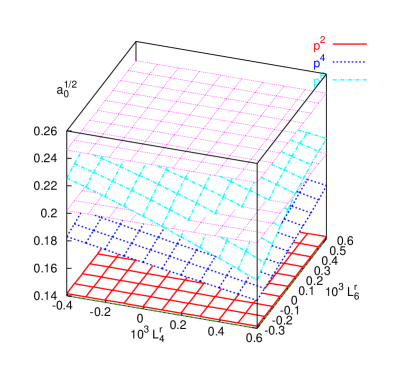
The results for $c^{+}_{10}$ and $c^{-}_{00}$, which are the only two that obtain a lowest order contribution, are shown in Figs. 3(a) and 3(b). $c^{-}_{00}$ has a large lowest order contribution and shows a reasonable convergence over the entire region of variation of $(L_{4}^{r},L_{6}^{r})$ we have covered. It is also in good agreement with the dispersive calculation inside the whole region. The result for $c^{+}_{10}$ shows somewhat less good convergence but it is still acceptable. This is what was used in earlier analyses of $\pi K$ scattering to get a determination of the $1/N_{c}$ suppressed constant $L_{4}^{r}$. As can be seen in Fig. 3(a) the matching with the dispersive values is obtained within the region $L_{4}^{r}\approx-0.1\,10^{-3}$ with only a fairly weak dependence on the value of $L_{6}^{r}$.

(a)

(b)

Figure 3: (a) The subthreshold parameter $c^{+}_{10}$ as a function of the input values of $L_{4}^{r}$ and $L_{6}^{r}$ used in the $L_{i}^{r}$ determination. The unlabeled planes are the result of [40] with their errors. (b) The same for the subthreshold parameter $c^{-}_{00}$.

The results for the other subthreshold parameters are more difficult to interpret. They show a variety of behaviours:i) some subthreshold parameters display indication of reasonable convergence while others obviously do not converge. ii) Some agree well with the dispersive values while others do so only for large values of $L_{4}^{r},L_{6}^{r}$. There is also no obvious pattern to which values for $L_{4}^{r},L_{6}^{r}$ gives the best agreements. Some of these difficulties could be due to the fact that the lowest order is small in the region relevant for the subthreshold expansion as can be seen in Figs. 1 and 2.

We now discuss some of them to show these issues also considering their agreement with the dispersive calculation. The latter can also be judged from Tab. 3. The $c^{+}_{00}$ component agrees with the dispersive result in a very small region for large negative $L_{4}^{r}$. That was precisely the place where the $\chi^{2}$ of the fits for the input parameters started getting large. $c^{+}_{20}$ agrees excellently at order $p^{4}$ but gets fairly large $p^{6}$ corrections. It starts agreeing once more for larger positive values of $L_{4}^{r}$ and $L_{6}^{r}$ than considered here. $c^{-}_{10}$ had a large negative estimate of the contribution from the $p^{6}$ constants. This drives the total $p^{6}$ contribution to be negative and the total result stays between 0.04 and 0.15, significantly below the dispersive result of [40]. The remaining subthreshold parameters all have large $p^{6}$ corrections and it is not clear whether we have a convergent series or not. But the general size and the sign is correct.

We now turn to the scattering lengths. The kinematical quantities here have values which are already large for ChPT but looking at Figs. 1 and 2 the convergence seems fine in that region. The finer features like higher partial waves and the radii might however work less well.

(a)

(b)

Figure 4: (a) The scattering length $a^{1/2}_{0}$ as a function of the input values of $L_{4}^{r}$ and $L_{6}^{r}$ used in the $L_{i}^{r}$ determination. The unlabeled planes are the result of [40] with their errors. (b) The same for the scattering length $a^{3/2}_{0}$.

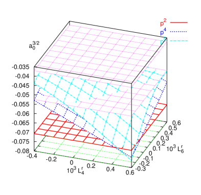
In Fig. 4(a) we have plotted the $S$ wave scattering length in the isospin 1/2 channel. The series shows a nice convergence and agrees with the dispersive result for most of the $L_{4}^{r}$-$L_{6}^{r}$ region we considered. Only a small region of negative $L_{6}^{r}$ and positive $L_{4}^{r}$ disagrees. The result for the $S$ wave scattering length in the $I=3/2$ channel, shown in Fig, 4(b), has qualitatively the same behaviour, ruling out a somewhat larger region of the $(L_{4}^{r},L_{6}^{r})$ plane. For the $P$ wave scattering lengths, we get agreement in the $I=1/2$ channel with the dispersive result in essentially the whole region considered with a preference for positive values of $L_{4}^{r}$. The $I=3/2$ channel, $a^{3/2}_{1}$ has large $p^{6}$ corrections always leading to a value significantly above the dispersive result. Looking at higher threshold parameters the picture is again mixed. $b^{1/2}_{0}$ is typically 40 to 60% above the dispersive result, $b^{3/2}_{0}$ is too small by 20 to 50% and $b_{1}^{1/2}$ and $b^{3/2}_{1}$ have obvious convergence problems. We have shown the results for fit 10 of [45] in Tab. 4 together with dispersive estimates of [40].

	Fit 10	[40]
$a^{1/2}_{0}$	0.220	$0.224\pm 0.022$
$10a^{1/2}_{1}$	0.18	$0.19\pm 0.01$
$10a^{3/2}_{0}$	$-0.47$	$-0.448\pm 0.077$
$10^{2}a^{3/2}_{1}$	0.31	$0.065\pm 0.044$
$10b^{1/2}_{0}$	1.3	$0.85\pm 0.04$
$10b^{3/2}_{0}$	$-0.27$	$-0.37\pm 0.03$
$T^{+}_{CD}$	2.11	$3.90\pm 1.50$

Table 4: The results for the scattering lengths and ranges and the amplitude at the Cheng-Dashen point as well as the dispersive result. The scattering lengths and ranges are given in units of $m_{\pi^{+}}$.

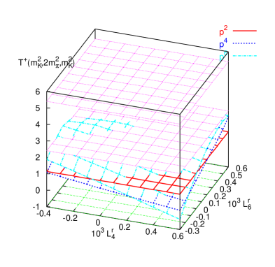
The value of the amplitude at the Cheng-Dashen point is related to the kaon sigma term. The dependence on $L_{4}^{r}$ and $L_{6}^{r}$ is shown in Fig. 5 together with the dispersive result of [40]. The corrections are large over most of the region and can be compared with the direct calculation of the sigma term shown in Fig. 9(b) of [19].

The overall picture we thus obtain in the end is rather mixed. If we look only at the quantities, $c^{+}_{10}$, $c^{-}_{00}$, $a_{0}^{1/2}$ and $a_{0}^{3/2}$ we see a series that converges reasonably well and reasonable agreement with the dispersive result from [40] is found for large regions of the values in the $(L_{4}^{r},L_{6}^{r})$ plane. In particular the value with $(L_{4}^{r},L_{6}^{r})\sim(0,0)$, corresponding to fit 10 of [53], is located inside the allowed region. The other quantities present more difficult to interpret results depending on how one judges their convergence and the (dis)agreement with the dispersive results of [40].

Figure 5: The amplitude at the Cheng-Dashen point as a function of the input values of $L_{4}^{r}$ and $L_{6}^{r}$ together with the dispersive estimates of [40].

8.2 $\pi K$, $\pi\pi$ and Scalar Form-factors

Even though it seems that the $\pi K$ processes alone do not provide strong restrictions on the low-energy constants we can use it together with $\pi\pi$ scattering and the scalar form-factor to restrict the region in the $(L_{4}^{r},L_{6}^{r})$ plane allowed. A full analysis is planned for the future but here we discuss the present results together with the earlier ones of [19, 18].

The constraints in the $(L_{4}^{r},L_{6}^{r})$ plane come from several sources:

1. The region inferred by the scalar form-factor analysis of [19].

$$L_{6}^{r}\approx L_{4}^{r}-0.35\,10^{-3}\,.$$ (35)

This came from two arguments: (i) The assumption that the pion and kaon isoscalar scalar form-factors at zero do not deviate by large factors from their lowest order values, as judged from Figs. 9(a) and 9(b) in [19]. (ii) The agreement of the ChPT calculation of the pion scalar radius with the dispersive results. Notice that the dispersive results used the values of the form-factors at zero as input. The ChPT prediction for the radius alone was rather constant as shown in Fig. 11(a) in [19].

2. From $\pi\pi$ scattering [18] we got constraints from four sources. The parameters $C_{1}$ and $C_{2}$ of [12] similar to subthreshold parameters and the scattering lengths $a^{0}_{0}$ and $a^{2}_{0}$. The constraints are (a) $a_{0}^{0}$ agrees reasonably well over the whole region considered, see Fig. 4(a) in [18]. (b) $a_{0}^{2}$ gives the strongest constraints, see Fig. 4(b) in [18]. It requires

$$L_{4}^{r}\gtrsim 0.27\,10^{-3}+0.9\,L_{6}^{r}\,.$$ (36)

(c) $C_{1}$ imposes $L_{4}^{r}\gtrsim 0.2~{}10^{-3}$ and does not constrain $L_{6}^{r}$, see Fig. 5(a) in [18]. (d) $C_{2}$ does not provide significant more constraints than the above, note that the plot shown in [18] is erroneous.

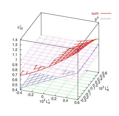
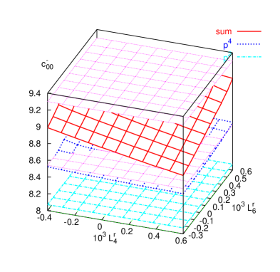
3. We review now the constraints we found in this article from $\pi K$ scattering. (a) $c_{00}^{-}$ imposes no constraint, see Fig. 3(b). (b) $c_{10}^{+}$, delimits

$$L_{4}^{r}\lesssim 0.28\,10^{-3}+0.25\,L_{6}^{r}\,,$$ (37)

see Fig. 3(a). (c) The constraint from $a_{0}^{1/2}$ is contained in the $a_{0}^{3/2}$, see Fig. 4(a). (d) The constraint from $a_{0}^{3/2}$, see Fig. 4(b), is $L_{6}^{r}\gtrsim L_{4}^{r}-0.4\,10^{-3}$.

Here we have used an error double the ones quoted in the dispersive results of [12, 40] to take the convergence of the chiral series somewhat into account as well.

The $\pi K$ constraint is essentially only from $c^{+}_{10}$, while for $\pi\pi$ scattering it is mainly $a^{2}_{0}$ with a little extra from $C_{1}$. These constraints do not overlap but the various regions almost touch for $L_{4}^{r}\approx 0.2\,10^{-3}$ and $L_{6}^{r}\lesssim 0.0\,10^{-3}$. At present the situation is only marginally compatible.

With the uncertainties associated in the calculations: the estimates of ${\cal O}(p^{6})$ LECs, correlations between the $L_{i}^{r}$ and the fact that the errors on the $L_{i}^{r}$ from $K_{\ell 4}$, the masses and decay constants is not yet taken into account the above conclusion is preliminary.

9 Conclusions

In this paper we have calculated the $\pi K$ scattering amplitude to next-to-next-to-leading order. We have presented analytically the results to next-to-leading order and the dependence on the $p^{6}$ LECs $C_{i}^{r}$. The remaining analytical expressions at order $p^{6}$ are very long and can be obtained from [50] or from the authors. This calculation is the main result of this work.

We presented some numerics with the LECs at order $p^{4}$ and $p^{6}$ set equal to zero at the scale of the rho mass. These results allow a first impression about the convergence of the series for various quantities, in particular we have presented results for the subthreshold parameters, the scattering lengths and the amplitude at the Cheng-Dashen point.

The second part of this work was a first attempt of extending the order $p^{4}$ work of constraining low-energy constants from $\pi K$ scattering of [40, 39, 58]. In these works values for $L_{4}^{r}$ were suggested that are positive and different from zero. We used in this work as inputs the correlated values for the $L_{i}^{r}$ determined from the $K_{\ell 4}$ form-factors, pseudoscalar meson masses and decay constants and estimated the contributions from the order $p^{6}$ constants with the same procedure as was used in previous next-to-next-to-leading processes. In contrast to the $p^{4}$ results, a first estimate for the quantities which appear to be most reliably obtainable from the $\pi K$ scattering amplitude at order $p^{6}$ are fully compatible with both the $1/N_{c}$ suppressed LECs $L_{4}^{r}$ and $L_{6}^{r}$ being equal to zero. Contrary to expectations, the study of these $\pi K$ (sub)threshold parameters alone do not allow to draw definite conclusions on the presence of large Zweig rule violating contributions as discussed in [15, 16] and references therein.

The remaining $\pi K$ quantities present a rather mixed picture, the convergence of the series is often questionable and the agreement with the results from the dispersive analysis is at the same level but no obvious large discrepancies exist. The estimated contribution of the $p^{6}$ constants to many quantities is fairly large and rather uncertain, especially those involving the scalars.

We have also studied how these results fit together with the earlier ones on $\pi\pi$ scattering and the scalar form-factors. We found only marginal compatibility as described in Sect. 8.2.

Planned work for the future is to combine all existing order $p^{6}$ calculations in three flavour ChPT in order to determine from experiment and/or dispersion theory as many as possible of the $p^{6}$ constants and to fully take into account all correlations for the $L_{i}^{r}$ and errors on the experimental and dispersive inputs used.