Interactions of Reggeized Gluons in the Möbius Representation
J. Bartels
Universität Hamburg
II. Institut für Theoretische Physik
Luruper Chaussee 149, D-22761 Hamburg, Germany;
L.N. Lipatov ^†
Petersburg Nuclear Physics Institute
Gatchina, 188 300 St.Petersburg, Russia
G.P. Vacca
INFN Bologna, Dipartimento di Fisica
Via Irnerio 46, I-40126 Bologna, Italy

Abstract

We investigate consequences of the Möbius invariance of the BFKL Hamiltonian and of the triple Pomeron vertex. In particular, we show that the triple Pomeron vertex in QCD, when restricted to the large $N_{c}$ limit and to the space of Möbius functions, simplifies and reduces to the vertex used in the Balitsky-Kovchegov (BK) equation. As a result, the BK equation for the dipole density appears as a special case of the nonlinear evolution equation which sums the fan diagrams for BFKL Green’s functions in the Möbius representation. We also calculate the corrections $O(1/(N_{c}^{2}-1)$ to the triple Pomeron vertex in the space of Möbius functions, and we present a generalization of the BK-equation in the next-to-leading order approximation in the $1/N_{c}$ expansion.

 

^(†) Humboldt Preisträger
Work supported in part by INTAS and by the Russian Fund of Fundamental Investigations

1 Introduction

It has been observed long time ago that the LO kernel of the BFKL equation  [1] is invariant under Möbius transformations  [2]. The same invariance holds for the transition vertex of $2\to 4$ reggeized gluons  [3]. This symmetry, together with the fact that, in physical scattering processes, the Green’s functions of reggeized gluons couple to impact factors of colorless projectiles which vanish as the momentum of any of the attached reggeized gluons goes to zero, leads to a freedom of redefining the Green’s functions of reggeized gluons. In particular, the Pomeron Green’s functions of two gluons in configuration space, $f(\mbox{\boldmath$\rho$}_{1},\mbox{\boldmath$\rho$}_{2})$, can be redefined to have the property $f(\mbox{\boldmath$\rho$},\mbox{\boldmath$\rho$})=0$. Functions of this type will be named as ‘being in the Möbius representation’ or, alternatively, as ‘belonging to the Möbius space of functions’.

In this paper we investigate some consequences of this Möbius representation for the interactions of reggeized gluons. After a brief review of the Möbius representation of solutions to the BFKL equation, we investigate the connection between the reggeon Green’s functions in the Möbius representation and the dipole picture  [4]. We then turn to the BKP equations  [5], and, finally, to the nonlinear equation of fan diagrams which, in the large $N_{c}$ limit, is shown to coincide with the Balitsky-Kovchegov equation  [6]. This equation is currently intensively studied in connection with saturation, and it has been rederived in the framework of different approaches [7].

We also compute the contribution of the non planar part of the transition vertex of $2\to 4$ reggeized gluons, which is subleading in $1/N_{c}$ and leads to a new contribution in the nonlinear equation for fan diagrams. We construct a system of coupled equations in the next-to-leading order approximation of the $1/N_{c}$ expansion.

2 Review of the BFKL Hamiltonian

To provide the conformal invariance of the BFKL equation [1] initially one should substitute the Born $t$-channel partial wave $f_{\omega}^{Born}$ ($\omega=j-1$), which is proportional to the product of two gluon Green functions $\ln\,\left|\rho_{11^{\prime}}\right|^{2}$ and $\ln\,\left|\rho_{22^{\prime}}\right|^{2}$, by the function $f_{\omega}^{(0)}$ of anharmonic ratios [2]

$$\frac{1}{\omega}\ln\,\left|\rho_{11^{\prime}}\right|^{2}\,\ln\,\left|\rho_{22^{\prime}}\right|^{2}\rightarrow f_{\omega}^{(0)}(\mbox{\boldmath$\rho$}_{1},\mbox{\boldmath$\rho$}_{2},\mbox{\boldmath$\rho$}_{1^{\prime}},\mbox{\boldmath$\rho$}_{2^{\prime}})\,,\,\,$$ (1)

$$f_{\omega}^{(0)}(\mbox{\boldmath$\rho$}_{1},\mbox{\boldmath$\rho$}_{2};\mbox{\boldmath$\rho$}_{1^{\prime}},\mbox{\boldmath$\rho$}_{2^{\prime}})=\frac{2}{\omega}\,\ln\,\frac{\left|\rho_{11^{\prime}}\right|\left|\rho_{22^{\prime}}\right|}{\left|\rho_{12^{\prime}}\right|\left|\rho_{21^{\prime}}\right|}\,\ln\,\frac{\left|\rho_{11^{\prime}}\right|\left|\rho_{22^{\prime}}\right|}{\left|\rho_{12}\right|\left|\rho_{1^{\prime}2^{\prime}}\right|},$$ (2)

which is invariant under the Möbius transformation

$$\rho_{k}\rightarrow\frac{a\rho_{k}+b}{c\rho_{k}+d}$$ (3)

for arbitrary complex parameters $a,b,c$ and $d$. We used here the complex coordinates for the initial ($k=1,2$) and final ($k=1^{\prime},2^{\prime}$) gluons in the two-dimensional impact parameter space $\mbox{\boldmath$\rho$}=(x,y)$

$$\rho_{k}=x_{k}+iy_{k}\,,\,\,\rho_{k}^{\ast}=x_{k}-iy_{k}\,,\,\,\,\rho_{kl}=\rho_{k}-\rho_{l}\,.$$ (4)

Such a substitution can be justified by making use of the fact that the impact factors $\Phi^{(A,B)}$ of colliding colourless particles

$$\Phi_{q}^{A}(\mbox{\boldmath$\rho$}_{1},\mbox{\boldmath$\rho$}_{2})=e^{i\mbox{\boldmath$q$}(\mbox{\boldmath$\rho$}_{1}+\mbox{\boldmath$\rho$}_{2})/2}\int\frac{d^{2}k\,}{(2\pi)^{2}}\,e^{i\mbox{\boldmath$k$}\mbox{\boldmath$\rho$}_{12}}\,\Phi^{A}(\frac{\mbox{\boldmath$q$}}{2}+\mbox{\boldmath$k$},\frac{\mbox{\boldmath$q$}}{2}-\mbox{\boldmath$k$})\,,\,\,\mbox{\boldmath$k$}=\frac{\mbox{\boldmath$k$}_{1}-\mbox{\boldmath$k$}_{2}}{2}\,,$$ (5)

$$\Phi_{q^{\prime}}^{B}(\mbox{\boldmath$\rho$}_{1^{\prime}},\mbox{\boldmath$\rho$}_{2^{\prime}})=e^{-i\mbox{\boldmath$q^{\prime}$}(\mbox{\boldmath$\rho$}_{1^{\prime}}+\mbox{\boldmath$\rho$}_{2^{\prime}})/2}\int\frac{d^{2}k\,}{(2\pi)^{2}}\,e^{-i\mbox{\boldmath$k$}\mbox{\boldmath$\rho$}_{1^{\prime}2^{\prime}}}\,\Phi^{A}(\frac{\mbox{\boldmath$q^{\prime}$}}{2}+\mbox{\boldmath$k$},\frac{\mbox{\boldmath$q^{\prime}$}}{2}-\mbox{\boldmath$k$})\,,\,\,\mbox{\boldmath$k$}=\frac{\mbox{\boldmath$k$}_{1}-\mbox{\boldmath$k$}_{2}}{2}\,.$$ (6)

entering in the expression for the scattering amplitude at high energies $\sqrt{s}$ and fixed $t=-\mbox{\boldmath$q$}^{2}$ in the leading logarithmic approximation (LLA).

$$A(s,t)=is\int_{\sigma-i\infty}^{\sigma+i\infty}\frac{d\omega}{2\pi i}\,\,e^{\omega Y}\,\,f_{\omega}(t)\,,\,Y=\ln\,s\,,$$ (7)

$$\,T_{\omega}^{A,B}=f_{\omega}(t)\,\delta^{2}(q-q^{\prime})=\int\prod_{r=1,2,1^{\prime},2^{\prime}}d^{2}\rho_{r}\,\,\,\Phi_{q}^{A}(\mbox{\boldmath$\rho$}_{1},\mbox{\boldmath$\rho$}_{2})\,f_{\omega}(\mbox{\boldmath$\rho$}_{1},\mbox{\boldmath$\rho$}_{2};\mbox{\boldmath$\rho$}_{1^{\prime}},\mbox{\boldmath$\rho$}_{2^{\prime}})\,\,\Phi_{q^{\prime}}^{B}(\mbox{\boldmath$\rho$}_{1^{\prime}},\mbox{\boldmath$\rho$}_{2^{\prime}})$$ (8)

satisfy the relations [2]

$$\int d^{2}\rho_{1}\,\Phi_{q,q^{\prime}}^{A,B}(\mbox{\boldmath$\rho$}_{1},\mbox{\boldmath$\rho$}_{2})=\int d^{2}\rho_{2}\,\Phi_{q,q^{\prime}}^{A,B}(\mbox{\boldmath$\rho$}_{1},\mbox{\boldmath$\rho$}_{2})=0\,.$$ (9)

These relations are consequences of gauge invariance of the impact factors. In the momentum representation they simply read as follows:

$$\Phi^{(A,B)}(0,\mbox{\boldmath$k$}_{2})=\Phi^{(A,B)}(\mbox{\boldmath$k$}_{1},0)=0$$ (10)

The last property has the interpretation that the interaction of a gluon with a small transverse momentum is proportional to the vanishing total colour charge of the colliding particle.

Note, that in an accordance with Ref. [2] the partial wave $T_{\omega}^{A,B}$ includes the $\delta$-function $\delta^{2}(q-q^{\prime})$ corresponding to the momentum conservation in the cross channel, and the impact factors $\Phi^{(A,B)}(\mbox{\boldmath$\rho$}_{1},\mbox{\boldmath$\rho$}_{2})$ in the coordinate representation are obtained from the impact factors $\Phi^{(A,B)}(\mbox{\boldmath$k$}_{1},\mbox{\boldmath$k$}_{2})$ in the momentum representation by the Fourier transformation.

The partial wave $f_{\omega}(\mbox{\boldmath$\rho$}_{1},\mbox{\boldmath$\rho$}_{2};\mbox{\boldmath$\rho$}_{1^{\prime}},\mbox{\boldmath$\rho$}_{2^{\prime}})$   for the gluon-gluon scattering in LLA satisfies the BFKL equation [1]:

$$f_{\omega}(\mbox{\boldmath$\rho$}_{1},\mbox{\boldmath$\rho$}_{2};\mbox{\boldmath$\rho$}_{1^{\prime}},\mbox{\boldmath$\rho$}_{2^{\prime}})=f_{\omega}^{(0)}(\mbox{\boldmath$\rho$}_{1},\mbox{\boldmath$\rho$}_{2};\mbox{\boldmath$\rho$}_{1^{\prime}},\mbox{\boldmath$\rho$}_{2^{\prime}})-\frac{\bar{\alpha}_{s}}{2\omega}\,H_{12}\,f_{\omega}(\mbox{\boldmath$\rho$}_{1},\mbox{\boldmath$\rho$}_{2};\mbox{\boldmath$\rho$}_{1^{\prime}},\mbox{\boldmath$\rho$}_{2^{\prime}})\,,$$ (11)

where $\bar{\alpha}_{s}=\alpha_{s}N_{c}/\pi$. The BFKL Hamiltonian $H_{12}$ in the leading logarithmic approximation (LLA) can be written in the operator form (see [12]):

$$H_{12}=\ln\,\left|p_{1}\right|^{2}+\ln\,\left|p_{2}\right|^{2}+\frac{1}{p_{1}p_{2}^{\ast}}\ln\,\left|\rho_{12}\right|^{2}\,p_{1}p_{2}^{\ast}\,+\frac{1}{p_{1}^{\ast}p_{2}}\ln\,\left|\rho_{12}\right|^{2}\,p_{1}^{\ast}p_{2}-4\Psi(1)\,,$$ (12)

where $\Psi(x)=d\ln\Gamma(x)/dx$, and we introduced the gluon holomorphic momenta

$$p_{r}=i\frac{\partial}{\partial\rho_{r}}\,,\,\,p_{r}^{\ast}=i\frac{\partial}{\partial\rho_{r}^{\ast}}\,.$$ (13)

It is important that the BFKL equation is implied to be projected to the class of functions $\widetilde{\Phi}(\mbox{\boldmath$p$}_{1},\mbox{\boldmath$p$}_{2})$ vanishing at $\mbox{\boldmath$p$}_{1}=0$ and $\mbox{\boldmath$p$}_{2}=0$ [2]. Because the function

$$\widetilde{\widetilde{\Phi}}(\mbox{\boldmath$p$}_{1},\mbox{\boldmath$p$}_{2})=\widetilde{\Phi}(\mbox{\boldmath$p$}_{1},\mbox{\boldmath$p$}_{2})H_{12}$$ (14)

also has the same properties, we conclude that the solution of the homogeneous BFKL equation

$$E\,f(\mbox{\boldmath$\rho$}_{1},\mbox{\boldmath$\rho$}_{2})=H_{12}\,\,f(\mbox{\boldmath$\rho$}_{1},\mbox{\boldmath$\rho$}_{2})\,,\,\,E=-\,\frac{2}{\bar{\alpha}_{s}}\,\omega\,.\,$$ (15)

is invariant under the substitution

$$f(\mbox{\boldmath$\rho$}_{1},\mbox{\boldmath$\rho$}_{2})\rightarrow\tilde{f}(\mbox{\boldmath$\rho$}_{1},\mbox{\boldmath$\rho$}_{2})=f(\mbox{\boldmath$\rho$}_{1},\mbox{\boldmath$\rho$}_{2})+f^{(1)}(\mbox{\boldmath$\rho$}_{1})+f^{(2)}(\mbox{\boldmath$\rho$}_{2})\,,$$ (16)

where $f^{(r)}(\mbox{\boldmath$\rho$}_{r})$ are arbitrary functions. One can use this freedom to impose the additional constraint on $f_{\omega}(\mbox{\boldmath$\rho$}_{1},\mbox{\boldmath$\rho$}_{2})$

$$\tilde{f}(\mbox{\boldmath$\rho$},\mbox{\boldmath$\rho$})=0\,,$$ (17)

by choosing $f^{(i)}(\mbox{\boldmath$\rho$}_{i})=-1/2f(\mbox{\boldmath$\rho$}_{i},\mbox{\boldmath$\rho$}_{i})$. We define the solutions having this property as functions belonging to the Möbius representation. This definition is in accordance with the fact that in such a class of functions the homogeneous BFKL equation is invariant under Möbius transformations.  Moreover, the conformal symmetry gives a possibility to find its solutions [2] in the form:

$$E_{m,\widetilde{m}}(\mbox{\boldmath$\rho$}_{1},\mbox{\boldmath$\rho$}_{2})=\left(\frac{\rho_{12}}{\rho_{10}\rho_{20}}\right)^{m}\left(\frac{\rho_{12}^{\ast}}{\rho_{10}^{\ast}\rho_{20}^{\ast}}\right)^{\widetilde{m}}$$ (18)

where the conformal weights $m$ and $\widetilde{m}$ are equal to

$$m=\frac{1}{2}+i\nu+\frac{n}{2}\,,\,\,\widetilde{m}=\frac{1}{2}+i\nu-\frac{n}{2}$$ (19)

for the principal series of unitary representations. They parametrize the eigenvalues of two Casimir operators of the global conformal group

$$M^{2}\,f_{m,\widetilde{m}}=m(m-1)\,f_{m,\widetilde{m}}\,,\,\,M^{\ast 2}\,f_{m,\widetilde{m}}=\widetilde{m}(\widetilde{m}-1)\,\,f_{m,\widetilde{m}}\,,$$ (20)

where

$$M^{2}=\left(\sum_{r=1}^{2}\mbox{\boldmath$M$}_{r}\right)^{2}=2\left(\mbox{\boldmath$M$}_{1},\mbox{\boldmath$M$}_{2}\right)=-\rho_{12}^{2}\partial_{1}\partial_{2}\,,\,\,\partial_{r}=\frac{\partial}{\partial\rho_{r}}\,.$$ (21)

Here $\mbox{\boldmath$M$}_{r}$ are the generators of the Möbius group

$$M_{r}^{3}=\rho_{r}\partial_{r}\,,\,\,M_{r}^{+}=\partial_{r}\,,\,\,M_{r}^{-}=-\rho_{r}\partial_{r}\,.$$ (22)

If we chose $f_{\omega}^{(0)}(\mbox{\boldmath$\rho$}_{1},\mbox{\boldmath$\rho$}_{2};\mbox{\boldmath$\rho$}_{1^{\prime}},\mbox{\boldmath$\rho$}_{2^{\prime}})$ as an inhomogeneous term of the BFKL equation, its solution is also conformally invariant [2] because the iteration of $\ f_{\omega}^{(0)}$ always gives functions belonging to the Möbius representation.

The BFKL Hamiltonian has the property of the holomorphic separability, [8]

$$H_{12}=h_{12}+h_{12}^{\ast},\,\,h_{12}=\sum_{r=1}^{2}\left(\ln p_{r}+\frac{1}{p_{r}}\ln(\rho_{12})\,p_{r}-\Psi(1)\right)\,.$$ (23)

This representation is valid in the space of Möbius functions, where terms proportional to $\delta^{(2)}(\rho_{12})$ (arising from $\nabla^{2}\log{|\rho|}=2\pi\delta^{(2)}(\rho)$) can be neglected. Alternatively, the holomorphic Hamiltonian $h_{12}$ can be written in another operator form [12]

$$h_{12}=\sum_{r=1}^{2}\left(\ln\rho_{12}+\rho_{12}\ln(p_{r})\frac{1}{\rho_{12}}-\Psi(1)\right)\,,$$ (24)

where we have used the relations

$$\log p=\frac{i}{\rho\,p}+\rho(\log{p})\,\frac{1}{\rho}\quad,\quad\frac{1}{p}(\log{\rho})\,p=-\frac{i}{\rho\,p}+\log\rho\,.$$ (25)

It means, that the total Hamiltonian $H_{12}$ can be presented as follows

$$H_{12}=2\ln\,\left|\rho_{12}\right|^{2}+\left|\rho_{12}\right|^{2}\ln\,\left|p_{1}p_{2}\right|^{2}\,\,\frac{1}{\left|\rho_{12}\right|^{2}}\,-4\,\Psi(1)\,,$$ (26)

where terms proportional to $\delta^{(2)}(\mbox{\boldmath$p$}_{i})$ have been neglected, since physical amplitudes have to be integrated with colourless impact factors. Finally, in the Möbius representation the Hamiltonian of the BFKL equation can be written as the integral operator:

$$H_{12}\,f_{\omega}(\mbox{\boldmath$\rho$}_{1},\mbox{\boldmath$\rho$}_{2})=\int\frac{d^{2}\rho_{3}}{\pi}\,\frac{\left|\rho_{12}\right|^{2}}{\left|\rho_{13}\right|^{2}\left|\rho_{23}\right|^{2}}\,\left(f_{\omega}(\mbox{\boldmath$\rho$}_{1},\mbox{\boldmath$\rho$}_{2})-f_{\omega}(\mbox{\boldmath$\rho$}_{1},\mbox{\boldmath$\rho$}_{3})-f_{\omega}(\mbox{\boldmath$\rho$}_{2},\mbox{\boldmath$\rho$}_{3})\right)\,.$$ (27)

Indeed, by introducing an intermediate ultraviolet regularization with $\delta\rightarrow 0$, we reproduce $H_{12}$ in the above operator form, because

$$\int\frac{d^{2}\rho_{3}}{\pi}\,\frac{\left|\rho_{12}\right|^{2}}{\left(\left|\rho_{13}\right|^{2}+\delta^{2}\right)\left(\left|\rho_{23}\right|^{2}+\delta^{2}\right)}=\int_{0}^{1}dx\frac{\left|\rho_{12}\right|^{2}}{x(1-x)\left|\rho_{12}\right|^{2}+\delta^{2}}\simeq 2\ln\,\frac{\left|\rho_{12}\right|^{2}}{\delta^{2}}\,,$$ (28)

$$- \!\left|\rho_{12}\right|^{2}\int\frac{d^{2}\rho_{3}}{\pi\left(\left|\rho_{23}\right|^{2}+\delta^{2}\right)}\,\frac{\,f_{\omega}(\mbox{\boldmath$\rho$}_{1},\mbox{\boldmath$\rho$}_{3})}{\left|\rho_{13}\right|^{2}}\,\simeq\left|\rho_{12}\right|^{2}\left(\ln\,(\delta^{2}\left|p_{2}\right|^{2})-\,2\Psi(1)\right)\,\frac{\,f_{\omega}(\mbox{\boldmath$\rho$}_{1},\mbox{\boldmath$\rho$}_{2})}{\left|\rho_{12}\right|^{2}}\,\,,$$ (29)

$$- \!\left|\rho_{12}\right|^{2}\int\frac{d^{2}\rho_{3}}{\pi\left(\left|\rho_{13}\right|^{2}+\delta^{2}\right)}\,\frac{f_{\omega}(\mbox{\boldmath$\rho$}_{2},\mbox{\boldmath$\rho$}_{3})}{\left|\rho_{23}\right|^{2}}\,\simeq\left|\rho_{12}\right|^{2}\left(\ln\,(\delta^{2}\left|p_{1}\right|^{2})-\,2\Psi(1)\right)\,\frac{\,f_{\omega}(\mbox{\boldmath$\rho$}_{1},\mbox{\boldmath$\rho$}_{2})}{\left|\rho_{12}\right|^{2}}\,.$$

In this form, the BFKL Hamiltonian was presented first in the context of the dipole picture [4] (see also [6]). It is instructive to trace, following the path of transformations from eq. (12) and (23) to (24) and (26), the gluon reggeization and the real production terms (which are connected to each other due to the bootstrap relation). Starting from (12), (23), we consider the terms related to the reggeized gluon trajectory, $\log{|p_{r}|^{2}}$. The use of the relation eq. (25) takes us to the form $\left|\rho_{12}\right|^{2}\ln\,\left|p_{r}\right|^{2}\,\,\frac{1}{\left|\rho_{12}\right|^{2}}$ (apart from the terms $\frac{1}{\rho_{12}p_{r}}$ which cancel when combined with the corresponding terms from the real production). When applying the relation (29), these terms are identified with those pieces which, in the dipole approach, are obtained from the real production. In the same way, those terms which in (12), (23) are associated with the real production $\frac{1}{p_{1}p_{2}^{\ast}}\ln\,\left|\rho_{12}\right|^{2}\,p_{1}p_{2}^{\ast}\,+\frac{1}{p_{1}^{\ast}p_{2}}\ln\,\left|\rho_{12}\right|^{2}\,p_{1}^{\ast}p_{2}$ are transformed into the $2\ln\,\left|\rho_{12}\right|^{2}$ term (taking into account the cancellation mentioned previously). Finally, thanks to the relation in eq. (28), one finds that this term gives the virtual (one loop) contribution in the dipole picture. Thus, when going from the momentum space representation of the BFKL Hamiltonian to the dipole picture, one observes a (partial) exchange of the virtual and real contributions and of the U.V. and I.R. sectors, which corresponds to the duality transformation [9].

3 The Möbius representation and the dipole picture

In the dipole approach [4] one introduces the dipole distribution in a hadron as a function of the rapidity $Y=\ln\,s$, $N_{\mbox{\boldmath$\rho$}_{1},\mbox{\boldmath$\rho$}_{2}}$. The BFKL equation is written in the form:

$$\frac{dN_{\mbox{\boldmath$\rho$}_{1},\mbox{\boldmath$\rho$}_{2}}}{dY}=-\,\frac{\bar{\alpha}_{s}}{2}\int\frac{d^{2}\rho_{3}}{\pi}\,\frac{\left|\rho_{12}\right|^{2}}{\left|\rho_{13}\right|^{2}\left|\rho_{23}\right|^{2}}\,\left(N_{\mbox{\boldmath$\rho$}_{1},\mbox{\boldmath$\rho$}_{2}}-N_{\mbox{\boldmath$\rho$}_{1},\mbox{\boldmath$\rho$}_{3}}-N_{\mbox{\boldmath$\rho$}_{2},\mbox{\boldmath$\rho$}_{3}}\right).$$ (30)

$N_{\mbox{\boldmath$\rho$}_{1},\mbox{\boldmath$\rho$}_{2}}$ can be interpreted as the scattering amplitude of a color dipole ( e.g. a quark-antiquark pair). It gives the possibility to calculate the total cross-sections $\sigma_{t}$ at high energies $\sqrt{s}$:

$$\sigma_{t}=\int d^{2}\rho_{1}d^{2}\rho_{2}\,\int_{0}^{1}dx\,\left|\psi_{p}(\mbox{\boldmath$\rho$}_{1},\mbox{\boldmath$\rho$}_{2})\right|^{2}\,N_{\mbox{\boldmath$\rho$}_{1},\mbox{\boldmath$\rho$}_{2}}(Y)\,.$$ (31)

Here $\psi_{p}(\mbox{\boldmath$\rho$}_{1},\mbox{\boldmath$\rho$}_{2};x)$ denotes the wave function of the colourless state of the projectile, being a composite state of two quarks with transverse coordinates $\mbox{\boldmath$\rho$}_{1}$, $\mbox{\boldmath$\rho$}_{2}$ and longitudinal momentum fractions $x$, $1-x$.

In order to illustrate the connection  [10] between this cross section formula and the discussion presented above, we consider, as an example, the elastic scattering of two virtual photons with momentum transfer squared $t=-\mbox{\boldmath$q$}^{2}$. In leading order, the impact factor $\Phi^{\gamma^{*}}$ is simply given by a closed quark loop with the $t$-channel gluons being attached in all possible ways. Starting from Feynman diagrams in momentum space und taking suitable Fourier transforms one obtains the following form for the scattering amplitude (8)  [11]:

$$T^{\gamma^{*}\gamma^{*}}=is\int d^{2}\rho_{1}d^{2}\rho_{2}d^{2}\rho_{1}^{\prime}d^{2}\rho_{2}^{\prime}e^{i\mbox{\boldmath$q$}(\mbox{\boldmath$\rho$}_{1}+\mbox{\boldmath$\rho$}_{2})/2}\int_{0}^{1}dx\psi_{p_{2}}(\mbox{\boldmath$\rho$}_{12},x)^{*}\psi_{p_{1}}(\mbox{\boldmath$\rho$}_{12},x)$$

$$\tilde{G}(\mbox{\boldmath$\rho$}_{1},\mbox{\boldmath$\rho$}_{2};\mbox{\boldmath$\rho$}_{1^{\prime}},\mbox{\boldmath$\rho$}_{2^{\prime}};Y)$$

$$e^{-i\mbox{\boldmath$q$}(\mbox{\boldmath$\rho$}_{1}^{\prime}+\mbox{\boldmath$\rho$}_{2}^{\prime})/2}\int_{0}^{1}dx^{\prime}\psi_{p_{2}^{\prime}}(\mbox{\boldmath$\rho$}_{1^{\prime}2^{\prime}},x^{\prime})^{*}\psi_{p_{1}^{\prime}}(\mbox{\boldmath$\rho$}_{1^{\prime}2^{\prime}},x^{\prime})\,,$$ (32)

where $p_{1}$, $p_{1^{\prime}}$ ($p_{2}$, $p_{2^{\prime}}$) denote the transverse momenta of the incoming (outgoing) photons, $x$ and $x^{\prime}$ are the longitudinal momentum fractions inside the impact factors. $\psi_{p}$ is the wave function of the virtual photon with transverse momentum $p$. Its dependence on the transverse momentum is contained in a phase factor:

$$\psi_{p}(\mbox{\boldmath$\rho$},x)=\psi(\mbox{\boldmath$\rho$},x)e^{i(1-x)\mbox{\boldmath$p$}\mbox{\boldmath$\rho$}_{12}},$$ (33)

where $\psi(\mbox{\boldmath$\rho$},x)$ denotes the usual photon wave function used in the total cross section formula. $\tilde{G}$ stands for the following Fourier transform of the momentum space BFKL Green’s function of reggeized gluons, $G_{\omega}(\mbox{\boldmath$k$}_{1},\mbox{\boldmath$k$}_{2};\mbox{\boldmath$k$}_{1}^{\prime},\mbox{\boldmath$k$}_{2}^{\prime};Y)$:

$$\tilde{G}(\mbox{\boldmath$\rho$}_{1},\mbox{\boldmath$\rho$}_{2}\mbox{\boldmath$\rho$}_{1^{\prime}}\mbox{\boldmath$\rho$}_{2^{\prime}};Y)=\int d^{2}kd^{2}k^{\prime}e^{i\mbox{\boldmath$k$}\mbox{\boldmath$\rho$}_{12}}\left(1-e^{-i(\mbox{\boldmath$k$}+\frac{\mbox{\boldmath$q$}}{2})\mbox{\boldmath$\rho$}_{12}}\right)\left(1-e^{i(-\mbox{\boldmath$k$}+\frac{\mbox{\boldmath$q$}}{2})\mbox{\boldmath$\rho$}_{12}}\right)$$

$$G(\mbox{\boldmath$k$}+\frac{\mbox{\boldmath$q$}}{2},-\mbox{\boldmath$k$}+\frac{\mbox{\boldmath$q$}}{2};\mbox{\boldmath$k$}^{\prime}+\frac{\mbox{\boldmath$q$}}{2},-\mbox{\boldmath$k$}^{\prime}+\frac{\mbox{\boldmath$q$}}{2};Y)$$

$$e^{-i\mbox{\boldmath$k$}\mbox{\boldmath$\rho$}_{1^{\prime}2^{\prime}}}\left(1-e^{i(\mbox{\boldmath$k$}+\frac{\mbox{\boldmath$q$}}{2})\mbox{\boldmath$\rho$}_{1^{\prime}2^{\prime}}}\right)\left(1-e^{-i(-\mbox{\boldmath$k$}+\frac{\mbox{\boldmath$q$}}{2})\mbox{\boldmath$\rho$}_{1^{\prime}2^{\prime}}}\right)\,.$$ (34)

This leads to the following identification:

$$N_{\mbox{\boldmath$\rho$}_{1},\mbox{\boldmath$\rho$}_{2}}=\int d^{2}\rho_{1}^{\prime}d^{2}\rho_{2}^{\prime}\tilde{G}(\mbox{\boldmath$\rho$}_{1},\mbox{\boldmath$\rho$}_{2};\mbox{\boldmath$\rho$}_{1^{\prime}},\mbox{\boldmath$\rho$}_{2^{\prime}};Y)e^{-i\mbox{\boldmath$q$}(\mbox{\boldmath$\rho$}_{1}^{\prime}+\mbox{\boldmath$\rho$}_{2}^{\prime})/2}\int_{0}^{1}dx^{\prime}\psi_{p_{2}^{\prime}}(\mbox{\boldmath$\rho$}_{1^{\prime}2^{\prime}},x^{\prime})^{*}\psi_{p_{1}^{\prime}}(\mbox{\boldmath$\rho$}_{1^{\prime}2^{\prime}},x^{\prime})\,.$$ (35)

In particular, the dipole scattering amplitude $N_{\mbox{\boldmath$\rho$}_{1},\mbox{\boldmath$\rho$}_{2}}$ is not simply the Fourier transform of the momentum space Green’s function but contains extra phase factors written in (34). These factors garantee that $N_{\mbox{\boldmath$\rho$}_{1},\mbox{\boldmath$\rho$}_{2}}$ vanishes as $\mbox{\boldmath$\rho$}_{12}$ tends to zero.

Another way to see how the gauge freedom allows us move from one representation to the other can be summarized in the following way, which will be useful in the study of the resummed fan diagram structure. Let us call $\theta_{IR}$ the collection of phase factors which, in the impact factor of a photon which splits in a $q\bar{q}$ pair, ties the squared modulus of the wave function to the Green’s function (in eq.(34), $\theta_{IR}$ stands for the phase factors in the first line (upper impact factor) or in the lower line (lower impact factor)): these $\theta_{IR}$ factors are zero if one of the two gluon momenta vanishes, and it contains subtraction terms with a $\delta^{(2)}(\rho_{12})$ behavior in the coordinate representation. We also introduce the operator $\theta^{UV}$, related to the transformation introduced in eq. (16) which contains terms proportional to $\delta^{(2)}(\mbox{\boldmath$p$}_{i})$. Using a shorthand notation and omitting the spatial integrations, one may write:

$$\Phi G=|\psi|^{2}\theta_{IR}G=|\psi|^{2}\theta_{IR}\theta^{UV}G=|\psi|^{2}\theta^{UV}G=|\psi|^{2}\tilde{G}\,,$$ (36)

where $\theta^{UV}$ is chosen in order to kill the subtractions contained in $\theta_{IR}$.

Results of this example can easily be generalized. It is possible to prove that the solution of the Bethe-Salpeter equation for the Pomeron wave function $f(\mbox{\boldmath$\rho$}_{1},\mbox{\boldmath$\rho$}_{2};Y)$ in the Möbius representation coincides with the dipole distribution $N_{\mbox{\boldmath$\rho$}_{1},\mbox{\boldmath$\rho$}_{2}}(Y)$. Both functions satisfy the same BFKL equation, and they vanish at $\mbox{\boldmath$\rho$}_{1}=\mbox{\boldmath$\rho$}_{2}$. An advantage of using the Pomeron wave function $f(\mbox{\boldmath$\rho$}_{1},\mbox{\boldmath$\rho$}_{2};Y)$ in the Möbius representation lies in the fact that the amplitude for the scattering of colorless particles is expressed as a convolution of the impact factors $\Phi_{q}^{A,B}(\mbox{\boldmath$\rho$}_{1},\mbox{\boldmath$\rho$}_{2})$ and the Green function $f$ for reggeized gluon interactions. The vanishing of  $f(\mbox{\boldmath$\rho$}_{1},\mbox{\boldmath$\rho$}_{2};Y)$ at $\mbox{\boldmath$\rho$}_{1}=\mbox{\boldmath$\rho$}_{2}$ means that, when performing the integration over $\mbox{\boldmath$\rho$}_{1}$ and $\mbox{\boldmath$\rho$}_{2}$, in the impact factor $\Phi_{q}(\mbox{\boldmath$\rho$}_{1},\mbox{\boldmath$\rho$}_{2})$ we can omit the terms proportional to $\delta^{2}(\rho_{12})$: these contributions correspond to those Feynman diagrams where the reggeized gluons are attached to the same quark or gluon line. As to the remaining Feynman diagrams in which the gluons are attached to different lines, their contributions can be expressed in terms of a colour density matrix $\Omega_{p_{1}p_{1^{\prime}}}(\mbox{\boldmath$\rho$}_{1},\mbox{\boldmath$\rho$}_{2})$

$$\Phi_{q}(\mbox{\boldmath$\rho$},\mbox{\boldmath$\rho^{\prime}$})\longrightarrow\Omega_{p_{1}p_{1^{\prime}}}(\mbox{\boldmath$\rho$},\mbox{\boldmath$\rho^{\prime}$})=$$ (37)

$$e^{i(\mbox{\boldmath$\rho$}+\mbox{\boldmath$\rho^{\prime}$})(\mbox{\boldmath$p$}_{1^{\prime}}-\mbox{\boldmath$p$}_{1})/2}\sum_{n}\int\prod_{k=1}^{n}dx_{k}\frac{d^{2}\rho_{k}}{2\pi}\,\,\psi_{p_{1^{\prime}}}^{\ast}\delta(1-\sum_{k=1}^{n}x_{k})\sum_{i\neq l}T_{i}^{a}T_{l}^{a}\,\delta^{2}(\rho_{i}-\rho)\,\delta^{2}(\rho_{l}-\rho^{\prime})\,\psi_{p_{1}}\,\,.$$ (38)

The wave functions $\psi_{p_{1}}$ and $\psi_{p_{1^{\prime}}}$ of the initial and final colourless particles contain the Fock states with an arbitrary number $n$ of gluons and quarks with longitudinal momenta $px_{k}$ and transverse coordinates $\mbox{\boldmath$\rho$}_{k}$. Due to the translational invariance they depend only on differences of $\mbox{\boldmath$\rho$}_{k}$.

The wave functions $\psi_{p_{r}}$ contain also a dependence on colour degrees of freedom of gluons and quarks. It is implied that the colour group generator $T_{i}^{a}$ acts on the colour indices of the parton $i$ and belongs to the corresponding representation of the colour group algebra $SU(N_{c})$. It means that only in the large-$N_{c}$ limit, where in color space the gluons can be visualized as being composite quark-antiquark states, the color density matrix is reduced to the dipole density. Note that, in general, the integrals over the variables $x_{k}$ are divergent at small values and should be regularized in order to avoid double-counting. Indeed, for the case of gluons the integration over the small-$x$ region is taken already into account in the BFKL resummation.

In LLA it is natural to leave in the parton wave functions for initial and final particles only the quark-antiquark component

$$\psi_{p_{r}}(\mbox{\boldmath$\rho$}_{1},\mbox{\boldmath$\rho$}_{2};x)=e^{i(\mbox{\boldmath$\rho$}_{1}+\mbox{\boldmath$\rho$}_{2},\mbox{\boldmath$p$}_{r})/2}\psi_{p_{r}}(\mbox{\boldmath$\rho$}_{12};x)\,.$$ (39)

Then the color density matrix is simplified

$$\Omega_{p_{1}p_{1^{\prime}}}(\mbox{\boldmath$\rho$},\mbox{\boldmath$\rho^{\prime}$})=e^{i(\mbox{\boldmath$\rho$}+\mbox{\boldmath$\rho^{\prime}$})(\mbox{\boldmath$p$}_{1^{\prime}}-\mbox{\boldmath$p$}_{1})/2}\,\frac{N_{c}^{2}-1}{2N_{c}}\int_{0}^{1}dx\,\,\psi_{p_{2}}^{\ast}(\mbox{\boldmath$\rho$}-\mbox{\boldmath$\rho^{\prime}$};x)\,\psi_{p_{1}}(\mbox{\boldmath$\rho$}-\mbox{\boldmath$\rho^{\prime}$};x)\,.$$ (40)

Therefore we obtain the dipole expressions discussed before.

Thus, in the Möbius representation both the reggeon and the dipole pictures are compatible with each other. In particular, in the reggeon language the fact that those diagrams where both reggeized gluons are attached to the same quark or gluon line (impulse approximation) give a vanishing contribution makes it natural for the BFKL Pomeron to be viewed as a Mandelstam cut. Indeed, for the Mandelstam cut the impact factor should contain only contributions of non-planar diagrams with non-zero third spectral function $\rho(s_{1},u_{1})$, whereas the diagrams of the impulse approximation do not contain singularities in one of two channels $s_{1}$ or $u_{1}$. Moreover, in QCD we can use the space-time picture for visualizing the Mandelstam cut as describing two independent parton fluctuations, produced by the high energy initial particle at $t\rightarrow-\infty$, long before the collision. The two fluctuations consist of large numbers of gluons which in the rapidity interval $0\leq y\leq\ln\,s$ are distributed homogeneously. The softest partons of each fluctuation interact simultaneously with the target. In this picture one can calculate not only the behaviour of total cross-sections, but, taking into account the AGK cutting rules, also the distribution of the produced particles inside the BFKL Pomerons. An important advantage of the reggeon approach over the dipole picture is the possibility of taking into account the non-trivial phase structure of reggeon diagrams related to their signature factors. The scattering amplitudes constructed in the framework of the reggeon calculus in QCD will satisfy the requirements of the $t$- and $s$- channel unitarities. In particular, $s$-channel unitarity is incorporated partly in the bootstrap relations for reggeon diagrams. In the dipole approach, both the bootstrap properties and $t$-channel unitarity remain somewhat obscure.

4 The BKP equations in the Möbius representation

The BFKL approach can be generalized to the case of colourless composite states constructed from $n$ reggeized gluons [5]. The homogeneous BKP equation for the $t$-channel partial wave in LLA has the form (see [12])

$$Ef=Hf\,,\,\,H=\sum_{1\leq k\leq l\leq n}\frac{T_{k}^{a}T_{l}^{a}}{(-N_{c})}H_{kl}\,,\,E=-\frac{2\pi}{\alpha_{c}N_{c}}\omega\,,$$ (41)

where $T_{k}^{a}$ are the colour group generators acting on colour indices of the gluon $k$. The spectrum of energies $E$ allows one to find the intercepts $\omega$ of the colourless reggeon bound states governing the corresponding contribution $\sim s^{\omega}$ to the total cross-section. The pair Hamiltonian $H_{kl}$ acting on the transverse coordinates of the reggeized gluons $\rho_{k},\rho_{k}^{\ast}$ can be written in the operator form [12]

$$H_{kl}=\ln\,\left|p_{k}\right|^{2}+\ln\,\left|p_{l}\right|^{2}+\frac{1}{p_{k}p_{l}^{\ast}}\ln\,\left|\rho_{12}\right|^{2}\,p_{k}p_{l}^{\ast}\,+\frac{1}{p_{k}^{\ast}p_{l}}\ln\,\left|\rho_{kl}\right|^{2}\,p_{k}^{\ast}p_{l}-4\Psi(1)\,.$$ (42)

Similar to the Pomeron case the BKP equation is implied to be multiplied by a smooth function $\widetilde{\Phi}$. We will assume that this function has a property of vanishing at small gluon momenta $\mbox{\boldmath$p$}_{r}$ ($r=1,2,...,n$). Similar to the Pomeron case one can verify that this property is conserved during the BFKL evolution. Therefore we have the freedom to add to $f$ a linear combination of functions which do not depend on one of coordinates $\mbox{\boldmath$\rho$}_{r}$. This gives the possibility to impose additional constraints on the solution $f$. In general, this freedom is not enough to find a solution $f$ which vanishes at small relative coordinates $\mbox{\boldmath$\rho$}_{rl}$. An example is the Odderon solution constructed from three reggeized gluons: some time ago we found a solution of the BKP equation $\ f(\mbox{\boldmath$\rho$}_{1},\mbox{\boldmath$\rho$}_{2},\mbox{\boldmath$\rho$}_{3})$, which is symmetric under the permutation $\mbox{\boldmath$\rho$}_{r}\longleftrightarrow\mbox{\boldmath$\rho$}_{l}$ but does not vanish at $\mbox{\boldmath$\rho$}_{rl}\rightarrow 0$ [16]. It is easy to see that by adding functions which do not depend on one of coordinates $\mbox{\boldmath$\rho$}_{s}$

$$\varphi(\mbox{\boldmath$\rho$}_{1},\mbox{\boldmath$\rho$}_{2},\mbox{\boldmath$\rho$}_{3})=f(\mbox{\boldmath$\rho$}_{1},\mbox{\boldmath$\rho$}_{2},\mbox{\boldmath$\rho$}_{3})+\tilde{f}(\mbox{\boldmath$\rho$}_{1},\mbox{\boldmath$\rho$}_{2})+\tilde{f}(\mbox{\boldmath$\rho$}_{2},\mbox{\boldmath$\rho$}_{3})+\tilde{f}(\mbox{\boldmath$\rho$}_{3},\mbox{\boldmath$\rho$}_{2})\,,$$ (43)

it is not possible to achieve $\varphi(\mbox{\boldmath$\rho$}_{1},\mbox{\boldmath$\rho$}_{2},\mbox{\boldmath$\rho$}_{3})=0$ at $\mbox{\boldmath$\rho$}_{r}=\mbox{\boldmath$\rho$}_{l}$, because $f(\mbox{\boldmath$\rho$}_{r},\mbox{\boldmath$\rho$}_{r},\mbox{\boldmath$\rho$}_{s})$ is not symmetric to the transmutation $\mbox{\boldmath$\rho$}_{r}\longleftrightarrow\mbox{\boldmath$\rho$}_{s}$.

Nevertheless, let us consider the class of solutions of the BKP equation, which are zero when one of the relative coordinates $\mbox{\boldmath$\rho$}_{rl}$ vanishes

$$\lim_{\mbox{\boldmath$\rho$}_{rl}\rightarrow 0}\,f=0\,.$$ (44)

We define such solutions as belonging to the (generalized) Möbius representation This definition is motivated by the fact, that for the functions in the Möbius representation the pair Hamiltonians $H_{kl}$ acts in the same space of functions as in the Pomeron case, and therefore it is Möbius invariant.  The property $f=0$ at $\mbox{\boldmath$\rho$}_{rl}=0$ is compatible with the BFKL evolution.

The fact, that in the Möbius representation the space of functions is universal, gives a possibility to find an upper boundary for the intercepts $\omega$ of composite states of $n$ reggeized gluons using a variational approach (cf. [13])

$$\omega\leq\frac{n(n-1)}{2}\,\omega_{BFKL}\,,$$ (45)

where

$$\omega_{BFKL}=\bar{\alpha}_{s}\,4\ln\,2\,.$$ (46)

In order to obtain this bound we have used a rather rough estimate, requiring that the average value of each pair Hamiltonian $H_{kl}$ is larger than the minimal eigenvalue $E_{BFKL}$ of the BFKL Hamiltonian.

In the Möbius representation the Hamiltonian $H$ has the property of holomorphic separability [8]

$$H=h+h^{\ast}\,,$$ (47)

where

$$h=\sum_{1\leq k\leq l\leq n}\frac{T_{k}^{a}T_{l}^{a}}{(-N_{c})}h_{kl}\,,\,\,h_{kl}=\sum_{r=k,l}\left(\ln(p_{r})+\frac{1}{p_{r}}\ln(\rho_{kl})p_{r}-\Psi(1)\right)\,.$$ (48)

However, the separability does not allow to simplify the BKP equation, because $h$ and $h^{\ast}$ do not commute with each other, due to the presence of the colour matrices. Only in the multi-colour limit $N_{c}\rightarrow\infty$ the colour structure is drastically simplified  [12]. Indeed, for a general irreducible case at $N_{c}\rightarrow\infty$ each gluon $r$ interacts with the neighbouring gluons $r+1$ and $r-1$, and the holomorphic and anti-holomorphic Hamiltonians $h,\,h^{\ast}\,$ commute with each other:

$$h=\frac{1}{2}\sum_{1\leq k\leq n}h_{k,k+1}\,,\,\,h^{\ast}=\frac{1}{2}\sum_{1\leq k\leq n}h_{k,k+1}\,,\,\,[h,h^{*}]=0\,.$$ (49)

Moreover, in the multi-colour limit there are many integrals of motion $q_{r}$ ($r=2,3,...,n$) [14]

$$q_{r}=\sum_{1\leq i_{1}\leq i_{2}....\leq i_{r}\leq n}\rho_{i_{1}i_{2}}\rho_{i_{2}i_{3}}...\rho_{i_{r}i_{1}\,\,}p_{i_{1}}p_{i_{2}}...p_{i_{r}}\,,\,\,[q_{r},q_{s}]=0\,,\,\,[q_{r},h]=0\,,$$ (50)

and the Hamiltonian $h$ coincides with the Hamiltonian for an integrable Baxter spin model.

5 Nonlinear equation for the fan diagrams

Let us now write down the evolution equation which sums the fan diagrams. To be definite, we consider a simplified model  [15] of the elastic scattering of two quark-antiquark pairs (Fig.1):

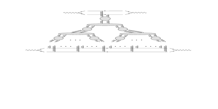
Figure 1: The fan diagram equation (the coupling of gluons to quark lines includes a sum over all possibilities).

the upper (smaller) quark pair couples to a single BFKL ladder , whereas the lower (larger) quark pair couples to an arbitrary number of BFKL Pomerons (Fig.1). Both couplings are taken to be of the eikonal type. As a consequence, at the lower quark pair the couplings of the BFKL Green’s functions factorize. When summing the fan diagrams, the transverse coordinates of the lower quark pair, $\mbox{\boldmath$\rho$}_{0}$, $\mbox{\boldmath$\rho$}_{0}^{\prime}$, are kept fixed. If $\Psi(\mbox{\boldmath$\rho$}_{1},\mbox{\boldmath$\rho$}_{2};\mbox{\boldmath$\rho$}_{0},\mbox{\boldmath$\rho$}_{0}^{\prime};Y)$ denotes the non-amputated two-gluon amplitude, the equation has the form:

$$\frac{\partial\Psi(\mbox{\boldmath$\rho$}_{1},\mbox{\boldmath$\rho$}_{2};\mbox{\boldmath$\rho$}_{0},\mbox{\boldmath$\rho$}_{0}^{\prime};Y)}{\partial Y}=-\frac{\bar{\alpha}_{s}}{2}(H_{12}\Psi)(\mbox{\boldmath$\rho$}_{1},\mbox{\boldmath$\rho$}_{2};\mbox{\boldmath$\rho$}_{0},\mbox{\boldmath$\rho$}_{0}^{\prime},Y)\hskip 56.9055pt$$

$$-\bar{\alpha}_{s}^{2}\int d^{2}\rho_{\alpha}d^{2}\rho_{\alpha^{\prime}}d^{2}\rho_{\beta}d^{2}\rho_{\beta^{\prime}}{\cal V}(\mbox{\boldmath$\rho$}_{1},\mbox{\boldmath$\rho$}_{2};\mbox{\boldmath$\rho$}_{\alpha},\mbox{\boldmath$\rho$}_{\alpha^{\prime}},\mbox{\boldmath$\rho$}_{\beta},\mbox{\boldmath$\rho$}_{\beta^{\prime}})\Psi(\mbox{\boldmath$\rho$}_{\alpha},\mbox{\boldmath$\rho$}_{\alpha^{\prime}};\mbox{\boldmath$\rho$}_{0},\mbox{\boldmath$\rho$}_{0}^{\prime};Y)\Psi(\mbox{\boldmath$\rho$}_{\beta},\mbox{\boldmath$\rho$}_{\beta^{\prime}};\mbox{\boldmath$\rho$}_{0},\mbox{\boldmath$\rho$}_{0}^{\prime};Y)\,,$$ (51)

where $H_{12}$ is the BFKL Hamiltonian, and ${\cal V}(\mbox{\boldmath$\rho$}_{1},\mbox{\boldmath$\rho$}_{2};\mbox{\boldmath$\rho$}_{\alpha},\mbox{\boldmath$\rho$}_{\alpha^{\prime}},\mbox{\boldmath$\rho$}_{\beta},\mbox{\boldmath$\rho$}_{\beta^{\prime}})$ denotes the conformal invariant $2\to 4$ transition vertex of reggeized gluons [17, 3, 18]. When supplemented with the initial condition:

$$\Psi(\mbox{\boldmath$\rho$}_{1},\mbox{\boldmath$\rho$}_{2};\mbox{\boldmath$\rho$}_{0},\mbox{\boldmath$\rho$}_{0}^{\prime};Y=0)=\alpha_{s}\;\left(f^{(0)}(\mbox{\boldmath$\rho$}_{1},\mbox{\boldmath$\rho$}_{2};\mbox{\boldmath$\rho$}_{0},\mbox{\boldmath$\rho$}_{0}^{\prime})+f^{(0)}(\mbox{\boldmath$\rho$}_{1},\mbox{\boldmath$\rho$}_{2};\mbox{\boldmath$\rho$}_{0}^{\prime},\mbox{\boldmath$\rho$}_{0})\right)\,,$$ (52)

where $f^{(0)}$ is proportional to the two gluon propagator in the Möbius representation, this nonlinear equation sums the fan diagrams coupled to the lower quark-antiquark pair. In order to obtain a physical scattering amplitude, we multiply $\Psi$ with suitable wave functions of external particles and integrate over the transverse coordinates $\mbox{\boldmath$\rho$}_{1}$, $\mbox{\boldmath$\rho$}_{2}$, $\mbox{\boldmath$\rho$}_{0}$, $\mbox{\boldmath$\rho$}_{0}^{\prime}$.

In the momentum space the $2\to 4$ transition vertex was found  [17] to consist of three pieces:

$$\bar{\alpha}_{s}^{2}{\cal V}(\mbox{\boldmath$q$}_{1},\mbox{\boldmath$q$}_{2};\mbox{\boldmath$k$}_{1},\mbox{\boldmath$k$}_{2},\mbox{\boldmath$k$}_{3},\mbox{\boldmath$k$}_{4})=\delta_{a_{1}a_{2}}\delta_{a_{3}a_{4}}V(1234)+\delta_{a_{1}a_{3}}\delta_{a_{2}a_{4}}V(1324)+\delta_{a_{1}a_{4}}\delta_{a_{2}a_{3}}V(1423)\,,$$ (53)

where we have introduced the short-hand notation

$$V(1234)=V(\mbox{\boldmath$q$}_{1},\mbox{\boldmath$q$}_{2};\mbox{\boldmath$k$}_{1},\mbox{\boldmath$k$}_{2},\mbox{\boldmath$k$}_{3},\mbox{\boldmath$k$}_{4}),$$ (54)

and the subscripts $a_{i}$ refer to the color degrees of the reggeized gluons. Obviously, the vertex $\cal V$ is completely symmetric under the exchange of any two gluon lines $i$ and $j$ $(i,j=1,2,3,4)$. Furthermore, the function $V(1234)$ vanishes if one of the four momenta $\mbox{\boldmath$k$}_{i}$ goes to zero. A convenient representation is the following:

$$V(1234)D_{2}=\frac{1}{2}g^{2}\Bigl{[}G(1,2+3,4)+G(2,1+3,4)+G(1,2+4,3)+G(2,1+4,3)$$

$$-G(1+2,3,4)-G(1+2,4,3)-G(1,2,3+4)-G(2,1,3+4)+G(1+2,0,3+4)\Bigr{]}\,.$$ (55)

The function $G(1,2,3)$ is the non-forward extension [18, 19] of the $G$-function introduced in [17]. It acts on the (amputated) 2-gluon test functions in the Möbius representation $D_{2}(\mbox{\boldmath$q$}_{1},\mbox{\boldmath$q$}_{2})$, and it consists of two pieces

$$G(\mbox{\boldmath$k$}_{1},\mbox{\boldmath$k$}_{2},\mbox{\boldmath$k$}_{3})=G_{1}(\mbox{\boldmath$k$}_{1},\mbox{\boldmath$k$}_{2},\mbox{\boldmath$k$}_{3})+G_{2}(\mbox{\boldmath$k$}_{1},\mbox{\boldmath$k$}_{2},\mbox{\boldmath$k$}_{3})\,,$$ (56)

The first term, $G_{1}$, belongs to the diagrams describing the emission of a real gluon,

$$G_{1}(\mbox{\boldmath$k$}_{1},\mbox{\boldmath$k$}_{2},\mbox{\boldmath$k$}_{3})=g^{2}N_{c}\,\int\frac{d^{2}\mbox{\boldmath$q$}_{1}d^{2}\mbox{\boldmath$q$}_{2}}{(2\pi)^{3}}\delta^{2}(\mbox{\boldmath$q$}_{1}+\mbox{\boldmath$q$}_{2}-\mbox{\boldmath$k$}_{1}-\mbox{\boldmath$k$}_{2}-\mbox{\boldmath$k$}_{3})D_{2}(\mbox{\boldmath$q$}_{1},\mbox{\boldmath$q$}_{2})$$

$$\left(\frac{(\mbox{\boldmath$k$}_{2}+\mbox{\boldmath$k$}_{3})^{2}}{(\mbox{\boldmath$q$}_{1}-\mbox{\boldmath$k$}_{1})^{2}\mbox{\boldmath$q$}_{2}^{2}}+\frac{(\mbox{\boldmath$k$}_{1}+\mbox{\boldmath$k$}_{2})^{2}}{\mbox{\boldmath$q$}_{1}^{2}(\mbox{\boldmath$q$}_{2}-\mbox{\boldmath$k$}_{3})^{2}}-\frac{\mbox{\boldmath$k$}_{2}^{2}}{(\mbox{\boldmath$q$}_{1}-\mbox{\boldmath$k$}_{1})^{2}(\mbox{\boldmath$q$}_{2}-\mbox{\boldmath$k$}_{3})^{2}}-\frac{(\mbox{\boldmath$k$}_{1}+\mbox{\boldmath$k$}_{2}+\mbox{\boldmath$k$}_{3})^{2}}{\mbox{\boldmath$q$}_{1}^{2}\mbox{\boldmath$q$}_{2}^{2}}\right),$$ (57)

whereas the second part is related to the virtual correction present in the reggeized gluon trajectory:

$$G_{2}(\mbox{\boldmath$k$}_{1},\mbox{\boldmath$k$}_{2},\mbox{\boldmath$k$}_{3}) = -\left[\omega(\mbox{\boldmath$k$}_{2})-\omega(\mbox{\boldmath$k$}_{2}+\mbox{\boldmath$k$}_{3})\right]D_{2}(\mbox{\boldmath$k$}_{1},\mbox{\boldmath$k$}_{2}+\mbox{\boldmath$k$}_{3})$$ (58)

$$-\left[\omega(\mbox{\boldmath$k$}_{2})-\omega(\mbox{\boldmath$k$}_{1}+\mbox{\boldmath$k$}_{2})\right]D_{2}(\mbox{\boldmath$k$}_{1}+\mbox{\boldmath$k$}_{2},\mbox{\boldmath$k$}_{3})\,.$$

The function $G(\mbox{\boldmath$k$}_{1},\mbox{\boldmath$k$}_{2},\mbox{\boldmath$k$}_{3})$ has the property to be zero for $\mbox{\boldmath$k$}_{1}=\mbox{\boldmath$0$}$ or $\mbox{\boldmath$k$}_{3}=\mbox{\boldmath$0$}$ (but not for $\mbox{\boldmath$k$}_{2}=\mbox{\boldmath$0$}$), so that one may easily see that the vertex $V(\mbox{\boldmath$k$}_{1},\mbox{\boldmath$k$}_{2},\mbox{\boldmath$k$}_{3},\mbox{\boldmath$k$}_{4})\rightarrow 0$ for any $\mbox{\boldmath$k$}_{i}\rightarrow\mbox{\boldmath$0$}$. This relation must be satisfied by any gauge invariant description of a t-channel 4-gluon state coupled to a colorless scattering projectile.

The expression in the coordinate representation was given in [18, 19] and can be written in terms of two non-local operators, $A_{1}$ and $A_{2}$. The operator $A_{1}$ is defined as follows:

$$G_{1}(\mbox{\boldmath$r$}_{1},\mbox{\boldmath$r$}_{2},\mbox{\boldmath$r$}_{3})=A_{1}D_{2}(\mbox{\boldmath$r$}_{1},\mbox{\boldmath$r$}_{3}),$$ (59)

and it has the following form:

$$A_{1}=\frac{g^{2}N_{c}}{8\pi^{3}}\Bigl{[}2\pi\delta^{2}(\mbox{\boldmath$r$}_{23})\partial_{3}^{2}(c-\ln r_{13})\partial_{3}^{-2}+2\pi\delta^{2}(\mbox{\boldmath$r$}_{12})\partial_{1}^{2}(c-\ln r_{13})\partial_{1}^{-2}$$

$$-2\frac{{\bf r}_{12}{\bf r}_{23}}{r_{12}^{2}r_{23}^{2}}-2\pi(c-\ln r_{13})(\delta^{2}(\mbox{\boldmath$r$}_{12})+\delta^{2}(\mbox{\boldmath$r$}_{23}))-4\pi^{2}\delta^{2}(\mbox{\boldmath$r$}_{12})\delta^{2}(\mbox{\boldmath$r$}_{23})(\mbox{\boldmath$\partial$}_{1}+\mbox{\boldmath$\partial$}_{3})^{2}\partial_{1}^{-2}\partial_{3}^{-2}\Bigr{]}\,.$$ (60)

Here $r_{ij}=|\mbox{\boldmath$r$}_{ij}|$, $\partial_{i}=|\mbox{\boldmath$\partial$}_{i}|$ and $c=\ln(2/m)+\psi(1)$, and $m$ is a gluon mass which provides an infrared regulator.

In order to transform $G_{2}$ to coordinate space, an ultraviolet regularization (with a parameter $\epsilon$) is necessary due to the presence of the gluon trajectory terms. The dependence on this regularization will disappear at the end. One obtains

$$G_{2}(\mbox{\boldmath$r$}_{1},\mbox{\boldmath$r$}_{2},\mbox{\boldmath$r$}_{3})=A_{2}D_{2}(\mbox{\boldmath$r$}_{1},\mbox{\boldmath$r$}_{3})\,,$$ (61)

where the operator $A_{2}$ is given by

$$A_{2} = -\frac{g^{2}N_{c}}{8\pi^{3}}\Bigl{[}\frac{1}{r_{23}^{2}}-2\pi c\delta^{2}(\mbox{\boldmath$r$}_{23})\Bigr{]}+\delta^{2}(\mbox{\boldmath$r$}_{23})\omega(-i\partial_{3})$$ (62)

$$-\frac{g^{2}N_{c}}{8\pi^{3}}\Bigl{[}\frac{1}{r_{12}^{2}}-2\pi c\delta^{2}(\mbox{\boldmath$r$}_{12})\Bigr{]}+\delta^{2}(\mbox{\boldmath$r$}_{12})\omega(-i\partial_{1})\,.$$

For the singular operators $1/r_{12}^{2}$ and $1/r_{23}^{2}$ one may use the ultraviolet regularization

$$\frac{1}{r^{2}}\equiv\frac{1}{r^{2}+\epsilon^{2}}+2\pi\delta^{2}(r)\ln\epsilon\,$$ (63)

with the understanding that $\epsilon\to 0$ at the end of the calculation. In the sum of the two operators, $A=A_{1}+A_{2}$, the terms containing $\ln m$ cancel, thus the dependence on the gluon mass disappears, and $G(\mbox{\boldmath$r$}_{1},\mbox{\boldmath$r$}_{2},\mbox{\boldmath$r$}_{3})=AD_{2}(\mbox{\boldmath$r$}_{1},\mbox{\boldmath$r$}_{3})$ is infrared stable.

6 Möbius representation for the fan equation

Let us now compare the fan diagram equation (51) with the Balitsky-Kovchegov equation (BK-equation)  [6]:

$$\frac{d}{dY}N_{\mbox{\boldmath$x$},\mbox{\boldmath$y$}}=\bar{\alpha}_{s}\int\frac{d^{2}z}{2\pi}\,\frac{\left|x-y\right|^{2}}{\left|x-z\right|^{2}\left|y-z\right|^{2}}\,\left(N_{\mbox{\boldmath$x$},\mbox{\boldmath$z$}}+N_{\mbox{\boldmath$y$},\mbox{\boldmath$z$}}-N_{\mbox{\boldmath$x$},\mbox{\boldmath$y$}}-N_{\mbox{\boldmath$x$},\mbox{\boldmath$z$}}N_{\mbox{\boldmath$y$},\mbox{\boldmath$z$}}\right)\,.$$ (64)

We will show that, by taking $N_{c}$ to be large and restricting ourselves to functions in the Möbius representation, the nonlinear fan diagram equation (51) coincides with the BK equation.

Beginning with the linear part of (51) which has been discussed in section 1, we make use of the freedom to add to the $\Psi(\mbox{\boldmath$\rho$}_{1},\mbox{\boldmath$\rho$}_{2})$ (which in the dipole approach is a symmetric function) a new function which depends only on one of the two coordinates. Moreover we scale the result by a factor proportional to $\alpha_{s}$. We choose

$$\tilde{\Psi}(\mbox{\boldmath$\rho$}_{1},\mbox{\boldmath$\rho$}_{2})=B\left(\Psi(\mbox{\boldmath$\rho$}_{1},\mbox{\boldmath$\rho$}_{2})-\frac{1}{2}\Psi(\mbox{\boldmath$\rho$}_{1},\mbox{\boldmath$\rho$}_{1})-\frac{1}{2}\Psi(\mbox{\boldmath$\rho$}_{2},\mbox{\boldmath$\rho$}_{2})\right)\,.$$ (65)

With this choice we have

$$\tilde{\Psi}(\mbox{\boldmath$\rho$},\mbox{\boldmath$\rho$})=0,$$ (66)

i.e. $\tilde{\Psi}$ is in the Möbius representation. Later on, we will identify $\tilde{\Psi}$ with the dipole distribution, $N$, and we will determine the constant $B$. The condition (66) is the color transparency relation (CTR). We remind that the shift (65) is allowed because of the ‘good’ properties of the impact factor which vanishes when either $\mbox{\boldmath$q$}_{1}=0$ or $\mbox{\boldmath$q$}_{2}=0$.

Let us now turn to the non-linear term in (51). As mentioned before, the $2\to 4$ gluon vertex is zero, when one of momenta $k_{i}$ tends to zero at fixed $q_{1}$ and $q_{2}$. This means that after performing the Fourier transformation of the equation and switching from the momenta $\mbox{\boldmath$k$}_{i}$ ($i=1,...,4$) to the coordinates $\mbox{\boldmath$\rho$}_{\alpha}$, $\mbox{\boldmath$\rho$}_{\alpha^{\prime}}$, $\mbox{\boldmath$\rho$}_{\beta}$, and $\mbox{\boldmath$\rho$}_{\beta^{\prime}}$ we are, again, allowed to add contributions to $\Psi(\mbox{\boldmath$\rho$}_{\alpha},\mbox{\boldmath$\rho$}_{\alpha^{\prime}})$ which lead to the condition $\tilde{\Psi}(\mbox{\boldmath$\rho$},\mbox{\boldmath$\rho$})=0$. They can be described by the projector $\theta^{UV}$ used in eq. (36). As a result, we have rewritten the fan diagram equation for $\Psi$ into an equation for $\tilde{\Psi}$ which belongs to the Möbius space of functions.

The final step now is the observation that, when projecting on color singlet states in the (12) and (34) subsystems, for large $N_{c}$, only the first term of (53), $V(1234)$, contributes. When acting on functions $\tilde{\Psi}(\mbox{\boldmath$\rho$}_{1},\mbox{\boldmath$\rho$}_{2})$ and $\tilde{\Psi}(\mbox{\boldmath$\rho$}_{3},\mbox{\boldmath$\rho$}_{4})$ which are in the Möbius representation, the second line of (55) does not contribute. For the remaining terms of $V(1234)$, the sum of the two operators $A_{1}$ and $A_{2}$ becomes simply

$$-4\frac{g^{2}}{2}\frac{g^{2}N_{c}}{8\pi^{3}}\frac{\rho_{12}^{2}}{\rho_{13}^{2}\rho_{23}^{2}}.$$ (67)

which coincides with the nonlinear term in the BK-equation, if we choose in eq. (65)

$$B=8\pi\bar{\alpha}_{s}.$$ (68)

Therefore, when identifying $N$ with our subtracted function (65), $\tilde{\Psi}$, the Balitsky-Kovchegov equation follows from the fan diagram equation, provided we restrict ourselves to the leading term at large $N_{c}$.

Next one may ask what kind of contribution is given by those terms in ${\cal V}(\mbox{\boldmath$q$}_{1},\mbox{\boldmath$q$}_{2};\mbox{\boldmath$k$}_{1},\mbox{\boldmath$k$}_{2},\mbox{\boldmath$k$}_{3},\mbox{\boldmath$k$}_{4})$, eq. (53), that we have neglected so far. In order to do that let us consider, inside a fan diagram, the splitting from a $\tilde{\Psi}^{\prime}$ state to a $\tilde{\Psi}\tilde{\Psi}$ state (we imagine that the subtraction $\Psi\to\tilde{\Psi}$ which guarantees $\tilde{\Psi}(\mbox{\boldmath$\rho$},\mbox{\boldmath$\rho$})=0$ has already been done). From the calculations shown in the appendix we derive the contribution:

$$\frac{2}{N_{c}^{2}-1}\!\!\!\!\!\!\! \!\!\!\!\!\!\int d^{2}\rho_{1}d^{2}\rho_{2}\frac{\alpha_{s}^{2}N_{c}}{\pi}\Biggl{\{}-2\frac{\tilde{\Psi}^{\prime}(\mbox{\boldmath$\rho$}_{1},\mbox{\boldmath$\rho$}_{2})}{|\mbox{\boldmath$\rho$}_{12}|^{4}}\int d^{2}\rho_{3}\frac{|\rho_{12}|^{2}}{|\rho_{13}|^{2}|\rho_{32}|^{2}}\tilde{\Psi}(\mbox{\boldmath$\rho$}_{1},\mbox{\boldmath$\rho$}_{3})\tilde{\Psi}(\mbox{\boldmath$\rho$}_{3},\mbox{\boldmath$\rho$}_{2})-$$ (69)

$$+ \frac{\tilde{\Psi}^{\prime}(\mbox{\boldmath$\rho$}_{1},\mbox{\boldmath$\rho$}_{2})}{|\mbox{\boldmath$\rho$}_{12}|^{4}}\left[-\pi H_{12}\tilde{\Psi}(\mbox{\boldmath$\rho$}_{1},\mbox{\boldmath$\rho$}_{2})\right]\tilde{\Psi}(\mbox{\boldmath$\rho$}_{1},\mbox{\boldmath$\rho$}_{2})+\tilde{\Psi}(\mbox{\boldmath$\rho$}_{1},\mbox{\boldmath$\rho$}_{2})\left[-\pi H_{12}\tilde{\Psi}(\mbox{\boldmath$\rho$}_{1},\mbox{\boldmath$\rho$}_{2})\right]+$$

$$+ \left[\frac{1}{|\mbox{\boldmath$\rho$}_{12}|^{4}}\pi H_{12}\tilde{\Psi}^{\prime}(\mbox{\boldmath$\rho$}_{1},\mbox{\boldmath$\rho$}_{2})\right]\tilde{\Psi}(\mbox{\boldmath$\rho$}_{1},\mbox{\boldmath$\rho$}_{2})\tilde{\Psi}(\mbox{\boldmath$\rho$}_{1},\mbox{\boldmath$\rho$}_{2})\Biggr{\}}\,.$$

It is now crucial to recall the hermitian symmetry of the BFKL Hamiltonian $H_{12}$ for the last term, according to

$$\int d^{2}\rho_{1}d^{2}\rho_{2}\left[\frac{1}{|\mbox{\boldmath$\rho$}_{12}|^{4}}\pi H_{12}\tilde{\Psi}^{\prime}(\mbox{\boldmath$\rho$}_{1},\mbox{\boldmath$\rho$}_{2})\right]\tilde{\Psi}^{2}(\mbox{\boldmath$\rho$}_{1},\mbox{\boldmath$\rho$}_{2})=\int d^{2}\rho_{1}d^{2}\rho_{2}\frac{\tilde{\Psi}^{\prime}(\mbox{\boldmath$\rho$}_{1},\mbox{\boldmath$\rho$}_{2})}{|\mbox{\boldmath$\rho$}_{12}|^{4}}\pi H_{12}\tilde{\Psi}^{2}(\mbox{\boldmath$\rho$}_{1},\mbox{\boldmath$\rho$}_{2})\,.$$ (70)

Performing the scaling by the factor $B$ which takes us from $\tilde{\Psi}$ to the dipole distribution $N_{\mbox{\boldmath$x$},\mbox{\boldmath$y$}}$ we find the simple form

$$\frac{1}{2}\frac{1}{N_{c}^{2}-1}\!\!\!\! \bar{\alpha}_{s} \!\!\!\!\int\frac{d^{2}z}{2\pi}\,\frac{\left|x-y\right|^{2}}{\left|x-z\right|^{2}\left|y-z\right|^{2}}\,\Biggl{[}-2N_{\mbox{\boldmath$x$},\mbox{\boldmath$z$}}N_{\mbox{\boldmath$z$},\mbox{\boldmath$y$}}+$$ (71)

$$+ 2\left(N_{\mbox{\boldmath$x$},\mbox{\boldmath$z$}}+N_{\mbox{\boldmath$z$},\mbox{\boldmath$y$}}-N_{\mbox{\boldmath$x$},\mbox{\boldmath$y$}}\right)N_{\mbox{\boldmath$x$},\mbox{\boldmath$y$}}-\left(N^{2}_{\mbox{\boldmath$x$},\mbox{\boldmath$z$}}+N^{2}_{\mbox{\boldmath$z$},\mbox{\boldmath$y$}}-N^{2}_{\mbox{\boldmath$x$},\mbox{\boldmath$y$}}\right)=$$

$$= \bar{\alpha}_{s}\int\frac{d^{2}z}{2\pi}\,\frac{\left|x-y\right|^{2}}{\left|x-z\right|^{2}\left|y-z\right|^{2}}\,\Biggl{[}-\frac{1}{2}\frac{1}{N_{c}^{2}-1}\left(N_{\mbox{\boldmath$x$},\mbox{\boldmath$z$}}+N_{\mbox{\boldmath$z$},\mbox{\boldmath$y$}}-N_{\mbox{\boldmath$x$},\mbox{\boldmath$y$}}\right)^{2}\Biggr{]}$$

The negative sign indicates that these large-$N_{C}$ corrections to the triple Pomeron vertex again lead to the saturation for evolution in rapidity. The factor $1/[2(N_{c}^{2}-1)]=1/16$ seems to suggest that this contribution should not play a crucial role. Nevertheless a direct investigation would be interesting.

It is important to note that, when going beyond the large $N_{c}$ limit, there are other corrections which slightly complicate the simple structure of the nonlinear fan diagram equation. They are due to the evolution of the colourless state of $2n$ reggeized gluons with $n>1$: for example, in leading order $1/N_{c}$, the four-gluon state consists of two noninterating Pomeron states. Each interaction between the Pomerons costs a suppression of the order $1/(N_{c}^{2}-1)$, i.e. it is of the same order as the corrections to the triple Pomeron vertex discussed above. Therefore, a consistent treatment of corrections beyond the large-$N_{c}$ limit has to include these corrections to the Hamiltonian of the evolution of four gluon state. As a first step, one can replace the single nonlinear evolution equation for $\tilde{\Psi}$ by a system of coupled equations, which describe the evolution of the two-gluon amplitude $\tilde{\Psi}$ and of the four-gluon Green’s function $G_{4}$. The equation for $N$ reads:

$$\frac{d}{dY}N_{\mbox{\boldmath$x$},\mbox{\boldmath$y$}}=\bar{\alpha}_{s}\int\frac{d^{2}z}{2\pi}\,\frac{\left|x-y\right|^{2}}{\left|x-z\right|^{2}\left|y-z\right|^{2}}\,\left(N_{\mbox{\boldmath$x$},\mbox{\boldmath$z$}}+N_{\mbox{\boldmath$y$},\mbox{\boldmath$z$}}-N_{\mbox{\boldmath$x$},\mbox{\boldmath$y$}}-N_{4}(\mbox{\boldmath$x$},\mbox{\boldmath$z$};\mbox{\boldmath$y$},\mbox{\boldmath$z$};Y)\right.$$

$$\left.-\frac{1}{2}\frac{1}{N_{c}^{2}-1}\left(N_{\mbox{\boldmath$x$},\mbox{\boldmath$z$}}+N_{\mbox{\boldmath$z$},\mbox{\boldmath$y$}}-N_{\mbox{\boldmath$x$},\mbox{\boldmath$y$}}\right)^{2}\right)$$ (72)

The argument structure of $N_{4}(\mbox{\boldmath$\rho$}_{1},\mbox{\boldmath$\rho$}_{2};\mbox{\boldmath$\rho$}_{3},\mbox{\boldmath$\rho$}_{4};Y)$ indicates that the first pair of gluons at positions $\mbox{\boldmath$\rho$}_{1}$, $\mbox{\boldmath$\rho$}_{2}$ are in a color singlet; the same applies to the second pair at $\mbox{\boldmath$\rho$}_{3}$, $\mbox{\boldmath$\rho$}_{4}$. In leading order $1/N_{c}$, $N_{4}(\mbox{\boldmath$\rho$}_{1},\mbox{\boldmath$\rho$}_{2};\mbox{\boldmath$\rho$}_{3},\mbox{\boldmath$\rho$}_{4};Y)$ equals the product $N_{\mbox{\boldmath$\rho$}_{1},\mbox{\boldmath$\rho$}_{2}}N_{\mbox{\boldmath$\rho$}_{3},\mbox{\boldmath$\rho$}_{4}}$. To include the first correction we write

$$N_{4}(\mbox{\boldmath$\rho$}_{1},\mbox{\boldmath$\rho$}_{2};\mbox{\boldmath$\rho$}_{3},\mbox{\boldmath$\rho$}_{4};Y)\;=\;N_{\mbox{\boldmath$\rho$}_{1},\mbox{\boldmath$\rho$}_{2}}N_{\mbox{\boldmath$\rho$}_{3},\mbox{\boldmath$\rho$}_{4}}+\Delta N_{4}(\mbox{\boldmath$\rho$}_{1},\mbox{\boldmath$\rho$}_{2};\mbox{\boldmath$\rho$}_{3},\mbox{\boldmath$\rho$}_{4};Y)$$ (73)

A second equation for $\Delta N_{4}$ describes the evolution of the four gluon Green’s function where the first interaction of the order $1/(N_{c}^{2}-1)$ between the two dipole cross sections $N$ is kept:

$$\frac{d}{dY}\Delta N_{4}(\mbox{\boldmath$\rho$}_{1},\mbox{\boldmath$\rho$}_{2};\mbox{\boldmath$\rho$}_{3},\mbox{\boldmath$\rho$}_{4};Y) = -\frac{\bar{\alpha}_{s}}{2(N_{c}^{2}-1)}\left(H_{12}+H_{34}\right)\left(N_{\mbox{\boldmath$\rho$}_{1},\mbox{\boldmath$\rho$}_{3}}N_{\mbox{\boldmath$\rho$}_{2},\mbox{\boldmath$\rho$}_{4}}+N_{\mbox{\boldmath$\rho$}_{1},\mbox{\boldmath$\rho$}_{4}}N_{\mbox{\boldmath$\rho$}_{2},\mbox{\boldmath$\rho$}_{3}}\right)$$ (74)

$$- \frac{\bar{\alpha}_{s}}{2}\left(H_{12}+H_{34}\right)\Delta N_{4}(\mbox{\boldmath$\rho$}_{1},\mbox{\boldmath$\rho$}_{2};\mbox{\boldmath$\rho$}_{3},\mbox{\boldmath$\rho$}_{4};Y)$$

When combined with the integral kernel in eq.(72), $\Delta N_{4}$ can be interpreted as a $O(1/N_{C}^{2})$ loop-correction to the triple Pomeron vertex in the space of Möbius functions. It would be interesting to study further correction terms of higher order in $O(1/N_{C}^{2})$.

7 Conclusions

In this paper we have investigated some consequences of the Möbius invariance of the BFKL Hamiltonian. When combined with the fact that Green’s functions of reggeized gluons couple to impact factors of colorless external states, this invariance allows to redefine the two-gluon Green’s function in such a way that it vanishes as the two coordinates of the gluons coincide. This property defines what we have named the ‘Möbius representation’. For the triple Pomeron vertex we have shown that this Möbius representation leads to a very simple form of the interaction kernel.

The use of the Möbius representation also allows to study the connection between the reggeon calculus in QCD (formulated in terms of t-channel partial waves) and the dipole picture. The latter is now widely been used for studies of, for example, saturation phenomena in deep inelastic scattering and in heavy ion collisions. An advantage of starting from the reggeon approach lies in the fact that it allows to go beyond the LO approximation and beyond the large-$N_{c}$ limit. As an example, we have studied the fan diagram equation. In the large-$N_{c}$ limit it coincides with the BK equation. We then have computed the $1/N_{c}^{2}$ suppressed corrections to the triple Pomeron vertex which are not contained in the BK equation. Accuracy of the order $1/N_{c}^{2}$ requires to consider also corrections in the evolution of the four gluon states; we propose a first modification of the BK equation which includes these corrections.

A few years ago the next-to-leading corrections (NLO) to the BFKL equation have been calculated in the framework of the reggeon approach [23]. Therefore it is natural to use these results in the Möbius representation and to study their role in the dipole picture.

8 Acknowledgments

G.P. Vacca and L.N. Lipatov wish to thank the II.Institüt für Theoretische Physik, University Hamburg, and DESY for the warm hospitality.

Appendix: The non planar contribution of the triple Pomeron vertex

Let us recall the structure of the two non-planar contributions to the vertex (53), $V(1324)$ and $V(1423)$. They have been studied previously in the context of the coupling of three pomeron states with definite conformal weights [20, 22, 21].

Each of them gives the same contribution, which can be derived from $V(1324)$:

$$V(1324)D_{2}=\frac{1}{2}g^{2}\Bigl{[}G(1,3+2,4)+G(3,1+2,4)+G(1,3+4,2)+G(3,1+4,2)$$

$$-G(1+3,2,4)-G(1+3,4,2)-G(1,3,2+4)-G(3,1,2+4)+G(1+3,0,2+4)\Bigr{]}\,.$$ (75)

First we note that, when coupling to color singlet states in the systems (12) and (34), these contributions are color suppressed by a factor $1/(N_{c}^{2}-1)$. Moreover one can immediately see that, when considering, due to the gauge freedom, functions $\tilde{\Psi}(\mbox{\boldmath$\rho$}_{1},\mbox{\boldmath$\rho$}_{2})$ in the Möbius representation, the second and third terms give no contribution. In the first and the fourth terms almost all the pieces cancel in the Möbius space of functions, and one is left with only two terms which in coordinate space have the form:

$$-\frac{\alpha_{s}^{2}N_{c}}{\pi(N_{c}^{2}-1)}\left(\delta^{(2)}(\mbox{\boldmath$\rho$}_{23})\frac{|\rho_{14}|^{2}}{|\rho_{13}|^{2}|\rho_{34}|^{2}}+\delta^{(2)}(\mbox{\boldmath$\rho$}_{14})\frac{|\rho_{13}|^{2}}{|\rho_{12}|^{2}|\rho_{23}|^{2}}\right)$$ (76)

When integrated with the $\tilde{\Psi}$ states. both pieces give the same contribution.

As to the last term in (75), when looking at the structure of $G$ it can be seen that the last term simply corresponds to a BFKL kernel acting on the amputated function $D_{2}$. However, in our fan resummation the vertex acts on non-amputated functions, and the term can be written as:

$$\frac{\alpha_{s}^{2}N_{c}}{\pi(N_{c}^{2}-1)}\delta^{(2)}(\mbox{\boldmath$\rho$}_{13})\delta^{(2)}(\mbox{\boldmath$\rho$}_{24})\frac{1}{|\rho_{12}|^{4}}\pi H_{12}$$ (77)

which acts on the single two gluon state before the splitting.

Let us finally consider the remaining four terms of (75) (the first four terms in the second line). Due to the fact that $G$ is an operator acting on the two gluon state (and not on the four gluon state), it is convenient to use an expression different from the previous form of the operators $A_{1}$ and $A_{2}$.

Namely, a direct investigation of, for example, $-G(1+3,2,4)$ gives:

$$\frac{\alpha_{s}^{2}N_{c}}{\pi(N_{c}^{2}-1)}\delta^{(2)}(\mbox{\boldmath$\rho$}_{13})\left[\frac{|\rho_{14}|^{2}}{|\rho_{12}|^{2}|\rho_{24}|^{2}}-\pi\log{|\rho_{14}|^{2}}\delta^{(2)}(\mbox{\boldmath$\rho$}_{34})\right]=\frac{\alpha_{s}^{2}N_{c}}{\pi(N_{c}^{2}-1)}\delta^{(2)}(\mbox{\boldmath$\rho$}_{13})Z^{1}_{4,2}.$$ (78)

Therefore it is easy to see that the action of this part of the non planar vertex reads

$$\int d^{2}\rho_{1}d^{2}\rho_{4}\frac{\alpha_{s}^{2}N_{c}}{\pi(N_{c}^{2}-1)}\frac{\bar{\Psi}^{\prime}(\mbox{\boldmath$\rho$}_{1},\mbox{\boldmath$\rho$}_{4})}{|\rho_{14}|^{4}}\!\!\!\!\!\!\!\!\!\!\!\!\!\! \Biggl{\{}\int d^{2}\rho_{3}\left[Z^{1}_{4,3}\tilde{\Psi}(\mbox{\boldmath$\rho$}_{1},\mbox{\boldmath$\rho$}_{3})+Z^{4}_{1,3}\tilde{\Psi}(\mbox{\boldmath$\rho$}_{3},\mbox{\boldmath$\rho$}_{4})\right]\tilde{\Psi}(\mbox{\boldmath$\rho$}_{1},\mbox{\boldmath$\rho$}_{4})+$$ (79)

$$+ \!\!\!\!\tilde{\Psi}(\mbox{\boldmath$\rho$}_{1},\mbox{\boldmath$\rho$}_{4})\int d^{2}\rho_{3}\left[Z^{1}_{4,3}\tilde{\Psi}(\mbox{\boldmath$\rho$}_{1},\mbox{\boldmath$\rho$}_{3})+Z^{4}_{1,3}\tilde{\Psi}(\mbox{\boldmath$\rho$}_{3},\mbox{\boldmath$\rho$}_{4})\right]\Biggr{\}}\,.$$

The integral operator depending on the kernel $Z^{i}_{j,k}$ in the two lines are simply BFKL kernel operators and can be written as

$$\int d^{2}\rho_{3}\left[Z^{1}_{4,3}\tilde{\Psi}(\mbox{\boldmath$\rho$}_{1},\mbox{\boldmath$\rho$}_{3})+Z^{4}_{1,3}\tilde{\Psi}(\mbox{\boldmath$\rho$}_{3},\mbox{\boldmath$\rho$}_{4})\right]=-\pi H_{14}\tilde{\Psi}(\mbox{\boldmath$\rho$}_{1},\mbox{\boldmath$\rho$}_{4})\,.$$ (80)

This form follows from the relation (29). We therefore conclude that the non planar vertex can be written in terms of well known objects.

References

• [1] L. N. Lipatov, Sov. J. Nucl. Phys23, 338 (1976); V. S. Fadin, E. A. Kuraev and L. N. Lipatov, Phys. Lett. B 60, 50 (1975); I. I. Balitsky and L. N. Lipatov, Sov. J. Nucl. Phys28, 822 (1978); JETP Lett30, 355 (1979).
• [2] L. N. Lipatov, Sov. Phys. JETP 63, (1986) 904.
• [3] J. Bartels, L. N. Lipatov and M. Wusthoff, Nucl. Phys. B 464 (1996) 298 [arXiv:hep-ph/9509303].
• [4] N.N. Nikolaev and B.G. Zakharov, Phys. Lett. B327 (1994) 149, 157; A.N. Mueller, Nucl. Phys. B415 (1994) 373.
• [5] J. Bartels, Nucl. Phys. B175 (1980) 365; J. Kwiecinski and M. Praszalowicz, Phys. Lett. B94 (1980) 413; T. Jaroszewicz, Acta Phys. Polon. B11 (1980) 965.
• [6] I.I. Balitsky, Nucl. Phys. B463 (1996) 99, Phys. Rev. D60 (1999) 014020; Y.V. Kovchegov, Phys. Rev. D60 (1999) 034008, Phys. Rev. D61 (2000) 074018.
• [7] See: I.I. Balitsky, “High-Energy QCD and Wilson Lines”, In *Shifman, M. (ed.): At the frontier of particle physics, vol. 2*, p. 1237-1342 (World Scientific, Singapore, 2001) [hep-ph/0101042]; E. Ferreiro, E. Iancu, A. Leonidov and L. McLerran, Nucl. Phys. A 703 (2002) 489 [arXiv:hep-ph/0109115]; and references therein.
• [8] L.N. Lipatov, Phys. Lett. B251 (1990) 284.
• [9] L.N.Lipatov, Nucl. Phys. B548 (1999) 328.
• [10] H.Navelet, S.Wallon, Nucl.Phys.B 522 (1998) 237.
• [11] J.Bartels, K.Golec-Biernat, K.Peters, Acta Phys.Polon.B34 (2003) 3051.
• [12] L.N. Lipatov, Phys. Lett. B309 (1993) 394;
• [13] P.Gauron, L.N.Lipatov, B.Nicolescu, Phys.Lett.B304 (1993) 334; Z.Phys.C63 (1994) 253
• [14] L.N. Lipatov, hep-th/9311037; DFPD/93/TH/70 (unpublished).
• [15] J. Bartels, M. Ryskin and G.P. Vacca, unpublished.
• [16] J. Bartels, L. N. Lipatov and G. P. Vacca, Phys. Lett. B 477 (2000) 178 [arXiv:hep-ph/9912423].
• [17] J. Bartels and M. Wusthoff, Z. Phys. C 66 (1995) 157.
• [18] M. A. Braun and G. P. Vacca, Eur. Phys. J. C 6 (1999) 147 [arXiv:hep-ph/9711486].
• [19] G. P. Vacca, PhD Thesis, arXiv:hep-ph/9803283.
• [20] H. Lotter, PhD Thesis, arXiv:hep-ph/9705288.
• [21] A. Bialas, H. Navelet and R. Peschanski, Phys. Lett. B 427 (1998) 147 [arXiv:hep-ph/9711236].
• [22] G. P. Korchemsky, Nucl. Phys. B 550 (1999) 397 [arXiv:hep-ph/9711277].
• [23] V. S. Fadin and L. N. Lipatov, Phys. Lett. B 429 (1998) 127; G. Camici and M. Ciafaloni, Phys. Lett. B 430 (1998) 349.