Vector-pseudoscalar two-meson distribution amplitudes in three-body $B$ meson decays

Abstract

We study three-body nonleptonic decays $B\to VVP$ by introducing two-meson distribution amplitudes for the vector-pseudoscalar pair, such that the analysis is simplified into the one for two-body decays. The twist-2 and twist-3 $\phi K$ two-meson distribution amplitudes, associated with longitudinally and transversely polarized $\phi$ mesons, are constrained by the experimental data of the $\tau\to\phi K\nu$ and $B\to\phi K\gamma$ branching ratios. We then predict the $B\to\phi K\gamma$ and $B\to\phi\phi K$ decay spectra in the $\phi K$ invariant mass. Since the resonant contribution in the $\phi K$ channel is negligible, the above decay spectra provide a clean test for the application of two-meson distribution amplitudes to three-body $B$ meson decays.

Viewing the experimental progress on three-body nonleptonic $B$ meson decays Belle ; Bar , it is urgent to construct a corresponding framework. In CL02 we have proposed a formalism based on the collinear factorization theorem in perturbative QCD (PQCD), in which new nonperturbative inputs, the two-meson distribution amplitudes, were introduced MP . On one hand, a direct evaluation of hard kernels for three-body decays, which contain two virtual gluons at lowest order, is not practical due to the enormous number of diagrams. On the other hand, the region with the two gluons being hard simultaneously is power-suppressed and not important. Therefore, the new nonperturbative inputs are necessary for catching dominant contributions in a simple manner. In our formalism the collinear factorization formula for a $B\to h_{1}h_{2}h_{3}$ decay amplitude is written, in general, as

$${\cal M}=\Phi_{B}\otimes H\otimes\Phi_{h_{1}h_{2}}\otimes\Phi_{h_{3}}\;,$$ (1)

where $\Phi_{B,h_{3}}$ are the $B,h_{3}$ meson distribution amplitudes, $\Phi_{h_{1}h_{2}}$ the $h_{1}h_{2}$ two-meson distribution amplitude, and $\otimes$ represents the convolution in longitudinal momentum fractions $x$. $\Phi_{h_{1}h_{2}}$ and $\Phi_{h_{3}}$ include not only the twist-2 (leading-twist), but two-parton twist-3 (next-to-leading-twist) components. The computation of the hard kernel $H$, basically the same as in two-body $B$ meson decays, is restricted to leading order in the coupling constant $\alpha_{s}$ so far.

There are two types of factorization theorems: collinear factorization BL ; BFL ; MR ; DM ; CZS and $k_{T}$ factorization BS ; NL . For a comparison of the two types of theorems, refer to Keum ; Li03 . Collinear factorization works, if it does not develop an end-point singularity from $x\to 0$. If it does, collinear factorization breaks down, and $k_{T}$ factorization is more appropriate. It has been known that collinear factorization of charmed and charmless two-body $B$ meson decays suffers the end-point singularities BBNS . This is the motivation to develop the PQCD formalism for two-body $B$ meson decays based on $k_{T}$ factorization YL ; KLS ; LUY . This approach has been shown to be infrared-finite, gauge-invariant, and consistent with the factorization assumption in the heavy-quark limit CLY ; LY1 ; LU . For three-body $B$ meson decays, the end-point singularities are smeared by the two-meson invariant mass CL02 , and collinear factorization in Eq. (1) holds. Moreover, it has been demonstrated that both nonresonant contributions and resonant contributions through two-body channels can be included by means of an appropriate parametrization of $\Phi_{h_{1}h_{2}}$ CL02 .

One of the challenges in the studies of three-body heavy meson decays is the evaluation of the matrix elements for heavy meson transition into two hadrons. There are already several theoretical approaches to this subject in the literature. The naive factorization BSW for three-body $B$ meson decays has been adopted in CHST , in which the $B$ meson transition into two hadrons was simply parameterized by a power-law behavior and then fit to experimental data. The matrix elements for the above transition were calculated using the pole model BFOPP ; cheng ; LGT , in which intermediate-state decays into two hadrons were described by effective weak and strong Lagrangians. The naive factorization has been improved in a so-called QCD-factorization framework W . However, only the current-produced amplitudes, i.e., those which can be expressed as products of two form factors in the factorization limit, were studied. The challenging subject of the $B$ meson transition into two hadrons was not addressed W . Compared to the above methods, our approach does not rely on the naive factorization, since the nonfactorizable contribution is taken into account through nonfactorizable hard kernels. It is complete in the sense that various topologies of amplitudes, such as the $B$ meson transition into two hadrons and the current-induced one, are analyzed in the same framework. It is also more systematic, because sub-leading corrections can be evaluated order by order in $\alpha_{s}$ and power by power in the ratios $w/m_{B}$ and $m_{h_{3}}/m_{B}$, where $w$ is the invariant mass of the two-meson system, and $m_{B}$ ($m_{h_{3}}$) the $B$ ($h_{3}$) meson mass.

In CL02 we have applied Eq. (1) to the modes, in which both $h_{1}$ and $h_{2}$ are pseudoscalar mesons $P$. The modes with $h_{1}$ being a vector meson $V$ and $h_{2}$ a pseudoscalar meson $P$ have been observed recently Bel03 . Hence, we shall extend our formalism to three-body decays involving the $B\to VP$ transition, taking $B\to\phi\phi K$ as an example. We shall first define the $\phi K$ two-meson distribution amplitudes, which are more complicated than the $PP$ ones. A simple parametrization is then proposed, and constrained by the experimental data of the $\tau\to\phi K\nu$ and $B\to\phi K\gamma$ branching ratios. Afterwards, we predict the decay spectra of the $B\to\phi K\gamma$ and $B\to\phi\phi K$ modes in the $\phi K$ invariant mass. The resonant contribution through the $\phi K$ channel is expected to be negligible: the $K_{1}(1650)$, $K_{2}(1770)$, and $K(1830)$ mesons decay into the $\phi K$ pair with the branching ratios not yet available in PDG . Therefore, the above spectra provide a clean test for the application of two-meson distribution amplitudes to three-body $B$ meson decays.

Label the momenta of the $\phi$ and $K$ mesons from the $B$ meson transition as $P_{1}$ and $P_{2}$, respectively. The $B$ meson momentum $P_{B}$ and the total momentum of the $\phi K$ pair, $P=P_{1}+P_{2}$, are chosen, in the light-cone coordinates, as

$$P_{B}=\frac{m_{B}}{\sqrt{2}}(1,1,{\bf 0}_{T})\;,\;\;\;\;P=\frac{m_{B}}{\sqrt{2}}(1,\eta,{\bf 0}_{T})\;,$$ (2)

with the variable $\eta=w^{2}/m_{B}^{2}$. Define $\zeta=P_{1}^{+}/P^{+}$ as the $\phi$ meson momentum fraction and $r_{\phi}=m_{\phi}/m_{B}$ as the $\phi$ meson-$B$ meson mass ratio, in terms of which the other kinematic variables are expressed as

$$P_{2}^{+}=(1-\zeta)P^{+}\;,\;\;\;\;P_{1}^{-}=[(1-\zeta)\eta+r_{\phi}^{2}]P^{+}\;,\;\;\;\;P_{2}^{-}=(\zeta\eta-r_{\phi}^{2})P^{+}\;,$$

$$P_{1}^{x}=-P_{2}^{x}=\sqrt{(\zeta w^{2}-m_{\phi}^{2})(1-\zeta)}\;,\;\;\;\;(P_{1}^{x})^{2}=(P_{2}^{x})^{2}\equiv P_{T}^{2}\;.$$ (3)

The polarization vectors $\epsilon(\phi)$ of the $\phi$ meson are obtained from the orthogonality $\epsilon(\phi)\cdot P_{1}=0$ and from the normalization $\epsilon(\phi)^{2}=-1$. The exact expressions are given, in the light-cone coordinates $\epsilon=(\epsilon^{+},\epsilon^{-},\epsilon^{x},\epsilon^{y})$, by

$$\epsilon_{L}(\phi) = \frac{1}{r_{\phi}}\left(\frac{\zeta[\zeta+(1-\zeta)\eta+r_{\phi}^{2}]-2r_{\phi}^{2}}{\sqrt{2}\sqrt{[\zeta+(1-\zeta)\eta+r_{\phi}^{2}]^{2}-4r_{\phi}^{2}}},\frac{[(1-\zeta)\eta+r_{\phi}^{2}][\zeta+(1-\zeta)\eta+r_{\phi}^{2}]-2r_{\phi}^{2}}{\sqrt{2}\sqrt{[\zeta+(1-\zeta)\eta+r_{\phi}^{2}]^{2}-4r_{\phi}^{2}}},\right.$$

$$\left.\frac{[\zeta+(1-\zeta)\eta+r_{\phi}^{2}]\sqrt{(\zeta\eta-r_{\phi}^{2})(1-\zeta)}}{\sqrt{[\zeta+(1-\zeta)\eta+r_{\phi}^{2}]^{2}-4r_{\phi}^{2}}},0\right)\;,$$

$$\epsilon_{T}^{(1)}(\phi) = \left(-\frac{\sqrt{2}\sqrt{(\zeta\eta-r_{\phi}^{2})(1-\zeta)}}{\sqrt{[\zeta+(1-\zeta)\eta+r_{\phi}^{2}]^{2}-4r_{\phi}^{2}}},\frac{\sqrt{2}\sqrt{(\zeta\eta-r_{\phi}^{2})(1-\zeta)}}{\sqrt{[\zeta+(1-\zeta)\eta+r_{\phi}^{2}]^{2}-4r_{\phi}^{2}}},\right.$$

$$\left.\frac{[\zeta-(1-\zeta)\eta-r_{\phi}^{2}]}{\sqrt{[\zeta+(1-\zeta)\eta+r_{\phi}^{2}]^{2}-4r_{\phi}^{2}}},0\right)\;,$$

$$\epsilon_{T}^{(2)}(\phi) = (0,0,0,1)\;.$$ (4)

The terms proportional to $r_{\phi}$ will be neglected eventually. The kaon is treated as a massless particle. The $\phi$ meson emitted from the weak vertex then carries the momentum $P_{3}=(m_{B}/\sqrt{2})(0,1-\eta,{\bf 0}_{T})$. Another equivalent, but more general, representation of $\epsilon(\phi)$ is given by

$$\epsilon^{\pm}_{L}(\phi) = \frac{P^{2}_{T}\pm P^{\pm}_{1}(P^{+}_{1}-P^{-}_{1})}{\sqrt{2}m_{\phi}p}\;,\;\;\;\;\epsilon_{L}^{x}(\phi)=\frac{P_{T}(P^{+}_{1}+P^{-}_{1})}{\sqrt{2}m_{\phi}p}\;,$$

$$\epsilon^{(1)\pm}_{T}(\phi) = \frac{\mp P_{T}}{\sqrt{2}p}\;,\;\;\;\;\ \ \ \epsilon^{(1)x}_{T}(\phi)=\frac{P^{+}_{1}-P^{-}_{1}}{\sqrt{2}p},$$ (5)

with $p=\sqrt{P^{2}_{T}+(P^{+}_{1}-P^{-}_{1})^{2}/2}$.

The three-body $B$ meson decays are dominated by the contribution from the region, in which the $\phi K$ pair possesses the invariant mass $w^{2}\sim O(\bar{\Lambda}m_{B})$ CL02 , $\bar{\Lambda}$ representing a hadronic scale. The orders of magnitude of the components,

$$P^{+}\sim O(m_{B})\;,\;\;\;\;P^{-}\sim O(\bar{\Lambda})\;,\;\;\;\;P_{T}\sim O(\sqrt{\bar{\Lambda}m_{B}})\;,$$ (6)

are then implied. It is easy to obtain the power counting rules of the polarization vectors from Eq. (4),

$$\epsilon_{L}^{+}(\phi)\sim\frac{1}{r_{\phi}}O(1)\;,\;\;\;\;\epsilon_{L}^{x}(\phi)\sim\frac{1}{r_{\phi}}O\left(\sqrt{\bar{\Lambda}/m_{B}}\right)\;,\;\;\;\;\epsilon_{L}^{-}(\phi)\sim\frac{1}{r_{\phi}}O(\bar{\Lambda}/m_{B})\;,$$

$$\epsilon_{T}^{(1)+}(\phi)\sim\epsilon_{T}^{(1)-}(\phi)\sim O\left(\sqrt{\bar{\Lambda}/m_{B}}\right)\;,\;\;\;\;\epsilon_{T}^{(1)x}(\phi)\sim O(1)\;.$$ (7)

In the heavy-quark limit the hierarchy $P^{+}\gg P_{T}\gg P^{-}$ corresponds to a collinear configuration, and suggests the employment of the new nonperturbative inputs, the $\phi K$ two-meson distribution amplitudes. For the $PP$ system, there is only a single twist-2 distribution amplitude associated with the structure $\gamma_{\mu}$, and two two-parton twist-3 distribution amplitudes associated with the structures $I$ (the identity) and $\sigma_{\mu\nu}$ CL02 ; MP ; M . Here a higher-twist distribution amplitude means that its contribution is suppressed by powers of $w/m_{B}$. For the $VP$ system, the relevant structures are more complicated: three twist-2 distribution amplitudes are associated with $\gamma_{\mu}\gamma_{5}$ and $\sigma_{\mu\nu}\gamma_{5}$, and five twist-3 distribution amplitudes with $\gamma_{\mu}\gamma_{5}$, $\sigma_{\mu\nu}\gamma_{5}$, $\gamma_{5}$ and $\gamma_{\mu}$. To decompose the two-meson distribution amplitudes into the components of different twists, we introduce the polarization vectors of the $\phi K$ system,

$$\epsilon_{L}=\frac{1}{\sqrt{2\eta}}(1,-\eta,0,0)\;,\;\;\;\;\epsilon_{T}^{(1)}=(0,0,1,0)\;,\;\;\;\;\epsilon_{T}^{(2)}=(0,0,0,1)\;.$$ (8)

A two-pion distribution amplitude has been related to the pion distribution amplitude through a perturbative calculation of the process $\gamma\gamma^{*}\to\pi^{+}\pi^{-}$ at large invariant mass $w^{2}$ DFK . In this work we adopt a similar trick: we calculate perturbatively the matrix elements,

$$\langle\phi(P_{1},\epsilon(\phi))K^{+}(P_{2})|\bar{u}(y^{-})\Gamma s(0)|0\rangle\;,$$ (9)

using the $\phi$ meson and kaon distribution amplitudes up to twist 3 PB1 ; PB2 , where $\Gamma$ represents a structure among $I$, $\gamma_{5}$, $\gamma_{\mu}$, $\gamma_{\mu}\gamma_{5}$ and $\sigma_{\mu\nu}\gamma_{5}$. The matrix elements can be expressed as the products of the corresponding form factors with the kinematic factors. For example, the matrix element for $\Gamma=\gamma_{\mu}\gamma_{5}$ is written as the product of the form factor $F_{\parallel}$ with the kinematic factor $(P_{1}-P_{2})_{\mu}$. The kinematic factors are then approximated in terms of the momentum $P$ and the polarization vectors $\epsilon$ of the $\phi K$ system according to the power counting rules in Eqs. (6) and (7). The resultant $\zeta$-dependent coefficients in the approximation contribute to the $\zeta$ dependence of the $\phi K$ two-meson distribution amplitudes.

We then derive the decomposition up to $O(w/m_{B})$,

$$\langle\phi K^{+}|\bar{u}(y^{-})\gamma_{\mu}\gamma_{5}s(0)|0\rangle = P_{\mu}\int_{0}^{1}dze^{izP\cdot y}\Phi_{\parallel}(z,\zeta,w)\;,$$ (10)

$$\langle\phi K^{+}|\bar{u}(y^{-})\sigma_{\mu\nu}\gamma_{5}s(0)|0\rangle = -i\left\{(\epsilon_{T\mu}P_{\nu}-\epsilon_{T\nu}P_{\mu})\int_{0}^{1}dze^{izP\cdot y}\Phi_{T}(z,\zeta,w)\right.$$ (11)

$$\left.+\frac{2}{w}(P_{1\mu}P_{2\nu}-P_{1\nu}P_{2\mu})\int_{0}^{1}dze^{izP\cdot y}\Phi_{3}(z,\zeta,w)\right\}\;,$$

$$\langle\phi K^{+}|\bar{u}(y^{-})\gamma_{5}s(0)|0\rangle = w\int_{0}^{1}dze^{izP\cdot y}\Phi_{p}(z,\zeta,w)\;,$$ (12)

$$\langle\phi K^{+}|\bar{u}(y^{-})\gamma_{\mu}s(0)|0\rangle = i\frac{w}{P\cdot n_{-}}\epsilon_{\mu\nu\rho\sigma}\epsilon_{T}^{\nu}P^{\rho}n_{-}^{\sigma}\int_{0}^{1}dze^{izP\cdot y}\Phi_{v}(z,\zeta,w)\;,$$ (13)

$$\langle\phi K^{+}|\bar{u}(y^{-})Is(0)|0\rangle = 0\;,$$ (14)

where $z$ is the momentum fraction carried by the spectator $u$ quark, and $n_{-}=(0,1,{\bf 0}_{T})$ a null vector. We have adopted the convention $\epsilon^{0123}=1$ for the Levi-Civita tensor $\epsilon^{\mu\nu\rho\delta}$. The above decomposition applies to other $VP$ systems, such as $K^{*}\pi$, $\rho K$, $\cdots$.

Below we present some details of the expansion of the kinematic factors. For Eq. (10), we have applied

$$(P_{1}-P_{2})_{\mu}\approx(2\zeta-1)P_{\mu}\;,$$ (15)

where the coefficient $2\zeta-1$ is absorbed into the distribution amplitude $\Phi_{\parallel}$, giving its $\zeta$ dependence. Similarly, we have approximated the kinematic factor for the matrix element in Eq. (11),

$$\epsilon_{T\mu}(\phi)P_{1\nu}-\epsilon_{T\nu}(\phi)P_{1\mu}\approx\zeta(\epsilon_{T\mu}P_{\nu}-\epsilon_{T\nu}P_{\mu})\;,$$ (16)

where the coefficient $\zeta$ is absorbed into $\Phi_{T}$, and $\epsilon_{T\mu}$ is a transverse polarization vector of the $\phi K$ system. The contribution from another distribution amplitude $\Phi_{3}$ can be combined with that from $\Phi_{T}$ via the approximation,

$$\frac{2}{w}\left(P_{1\mu}P_{2\nu}-P_{1\nu}P_{2\mu}\right)\approx 2\sqrt{\zeta(1-\zeta)}(\epsilon^{(1)}_{T\mu}P_{\nu}-\epsilon^{(1)}_{T\nu}P_{\mu})\;,$$ (17)

where the coefficient $\sqrt{\zeta(1-\zeta)}$ comes from $P_{1}^{x}$ in the $m_{\phi}\to 0$ limit. Since the branching ratio is a sum over the transverse polarizations $\epsilon^{(1)}_{T\mu}$ and $\epsilon^{(2)}_{T\mu}$, we omit the coefficient 2, and replace $\epsilon^{(1)}_{T\mu}$ by the two possible $\epsilon_{T\mu}$. We have employed the approximation for the matrix element in Eq. (13),

$$\frac{2}{w}\epsilon_{\mu\nu\rho\sigma}\epsilon_{T}^{\nu}(\phi)P_{1}^{\rho}P_{2}^{\sigma}\approx\frac{w}{P\cdot n_{-}}\zeta\epsilon_{\mu\nu\rho\sigma}\epsilon_{T}^{\nu}P^{\rho}n_{-}^{\sigma}\;.$$ (18)

For this structure, the $\phi$ meson emitted from the weak vertex must carry a transverse polarization, and a non-vanishing hard kernel demands that the subscript $\mu$ denotes a transverse component. The coefficient $\zeta$ is then the sum of $\zeta$, $\zeta-1$, and $1-\zeta$ from the combinations ($\epsilon_{T}^{(1)\nu}(\phi)=\epsilon_{T}^{(1)\perp}(\phi)$, $P^{\rho}=P^{+}$, $P_{2}^{\sigma}=P_{2}^{-}$), ($\epsilon_{T}^{(1)\nu}(\phi)=\epsilon_{T}^{(1)\perp}(\phi)$, $P^{\rho}=P^{-}$, $P_{2}^{\sigma}=P_{2}^{+}$), and ($\epsilon_{T}^{(1)\nu}(\phi)=\epsilon_{T}^{(1)-}(\phi)$, $P^{\rho}=P^{+}$, $P_{2}^{\sigma}=P_{2}^{\perp}$), respectively. A coefficient 2 for the last combination has been omitted for the same reason.

Our strategy does not provide the $z$ dependence. Assuming the $z$ dependence of each $\Phi_{i}(z,\zeta,w)$ to be asymptotic, we propose the parametrization,

$$\Phi_{\parallel}(z,\zeta,w) = \frac{3F_{\parallel}(w)}{\sqrt{2N_{c}}}z(1-z)(2\zeta-1)\;,\;\;\;\;$$

$$\Phi_{T}(z,\zeta,w) = \frac{3F_{T}(w)}{\sqrt{2N_{c}}}z(1-z)\zeta\;,\;\;\;\;$$

$$\Phi_{3}(z,\zeta,w) = \frac{3F_{3}(w)}{\sqrt{2N_{c}}}z(1-z)\;,$$

$$\Phi_{p}(z,\zeta,w) = \frac{3F_{p}(w)}{\sqrt{2N_{c}}}z(1-z)\;,$$

$$\Phi_{v}(z,\zeta,w) = \frac{3F_{v}(w)}{\sqrt{2N_{c}}}z(1-z)\zeta\;.$$ (19)

The time-like form factors $F_{\parallel,T,3,p,v}(w)$ define the normalization of the $\phi K$ two-meson distribution amplitudes. Note that these form factors are normalized to $F_{\parallel,T,3,p,v}(m_{\phi})=1$ in order to respect the kinematic threshold of decay spectra. Our strategy also reveals the power behaviors of the form factors in the asymptotic region with large $w$, $F_{\parallel,T}(w)\sim 1/w^{2}$ and $F_{3,p,v}(w)\sim m_{0}/w^{3}$, $m_{0}\approx 1.7$ GeV KLS ; HHZ being the chiral scale. Therefore, we further parameterize the form factors in the whole range of $w$ for the evaluation of the nonresonant contribution:

$$F_{\parallel}(w) = \frac{m_{\parallel}^{2}}{(w-m_{\phi})^{2}+m_{\parallel}^{2}}\;,$$

$$F_{T}(w) = \frac{m_{T}^{2}}{(w-m_{\phi})^{2}+m_{T}^{2}}\;,$$

$$F_{3}(w) = F_{p}(w)=\frac{m_{0}m_{\parallel}^{2}}{(w-m_{\phi})^{3}+m_{0}m_{\parallel}^{2}}\;,$$

$$F_{v}(w) = \frac{m_{0}m_{T}^{2}}{(w-m_{\phi})^{3}+m_{0}m_{T}^{2}}\;,$$ (20)

where the two free parameters $m_{\parallel,T}$, expected to be few GeV CL02 , are determined by the fit to the measured $\tau\to\phi K\nu$ and $B\to\phi K\gamma$ branching ratios PDG . The form factors depending on the parameter $m_{\parallel}$ ($m_{T}$) are associated with the longitudinally (transversely) polarized $\phi$ meson.

We stress that Eqs. (10) and (11) contain not only the twist-2 distribution amplitudes, but the twist-3 ones. The expansion in Eq. (15) corresponding to the component $\mu=\perp$ generates

$$w\epsilon_{T\mu}\int_{0}^{1}dze^{izP\cdot y}\Phi_{a}(z,\zeta,w)\;,$$

$$\Phi_{a}(z,\zeta,w)=\frac{3F_{\parallel}(w^{2})}{\sqrt{2N_{c}}}z(1-z)\sqrt{\zeta(1-\zeta)}\;.$$ (21)

Similarly, we extract two twist-3 distribution amplitudes from Eqs. (16) and (17) corresponding to the components $\mu,\nu=+,-$, given by

$$(\epsilon_{L\mu}P_{\nu}-\epsilon_{L\nu}P_{\mu})\int_{0}^{1}dze^{izP\cdot y}\left[(2\zeta-1)\Phi_{3}(z,\zeta,w)-\Phi_{t}(z,\zeta,w)\right]\;,$$

$$\Phi_{t}(z,\zeta,w)=\frac{3F_{T}(w^{2})}{\sqrt{2N_{c}}}z(1-z)\sqrt{\zeta(1-\zeta)}\;.$$ (22)

For the $\phi K$ system, the above twist-3 distribution amplitudes lead to smaller contributions compared to $\Phi_{p}$ and $\Phi_{v}$, and have been ignored: because of $m_{\phi}^{2}/w^{2}\sim 1$, the range in Eq. (28) below indicates $\zeta\sim 1$, and that the contribution from $\Phi_{a}$ is suppressed by the factor $\sqrt{1-\zeta}$. There exists a strong cancellation between $\Phi_{3}$ and $\Phi_{t}$ in Eq. (22). For other systems, such as $\rho K$, these twist-3 distribution amplitudes could be numerically important due to $m_{\rho}^{2}/w^{2}\ll 1$ in this case.

For the $B$ meson distribution amplitude, we use the model KLS ,

$$\Phi_{B}(x)=N_{B}x^{2}(1-x)^{2}\exp\left[-\frac{1}{2}\left(\frac{xm_{B}}{\omega_{B}}\right)^{2}\right]\;,$$ (23)

with the shape parameter $\omega_{B}=0.40\pm 0.04$ GeV TLS , and the normalization constant $N_{B}$ being related to the decay constant $f_{B}=190$ MeV (in the convention $f_{\pi}=130$ MeV) via $\int_{0}^{1}\Phi_{B}(x)dx=f_{B}/(2\sqrt{2N_{c}})$. The range of $\omega_{B}$ is determined from a fit to the values of the $B\to\pi$ form factor from light-cone sum rules KR ; PB3 . The above $\Phi_{B}$ is identified as $\Phi_{+}$ of the two leading-twist $B$ meson distribution amplitudes $\Phi_{\pm}$ defined in GN ; DS . Equation (23), vanishing at $x\to 0$, is consistent with the behavior required by equations of motion KKQT . It has been shown that the $B$ meson distribution amplitude is normalizable in $k_{T}$ factorization theorem LL04 , contrary to the conclusion drawn in the framework of collinear factorization theorem Neu03 ; BIK . Another distribution amplitude ${\bar{\Phi}}_{B}$, identified as ${\bar{\Phi}}_{B}=(\Phi_{-}-\Phi_{+})/\sqrt{2}$ with a zero normalization, contributes at the next-to-leading power of $\bar{\Lambda}/m_{B}$ TLS . It has been verified numerically LMY that the contribution to the $B\to\pi$ form factor from $\Phi_{B}$ is much larger than from ${\bar{\Phi}}_{B}$.

In summary, we calculate the hard kernels by contracting the quark-level diagrams with the matrix elements,

$$\langle 0|{\bar{b}}(0)_{l}d(y^{-})_{j}|B(P_{B})\rangle = \frac{1}{\sqrt{2N_{c}}}\int_{0}^{1}dxe^{-ixP\cdot y}[(\not{P}_{B}+m_{B})\gamma_{5}]_{lj}\Phi_{B}(x)\;,$$

$$\langle\phi K(P,\epsilon_{L})|\bar{u}(y^{-})_{j}s(0)_{l}|0\rangle = \frac{1}{\sqrt{2N_{c}}}\int_{0}^{1}dze^{izP\cdot y}\left\{(\gamma_{5}\not P)_{lj}\Phi_{\parallel}(z,\zeta,w)+(\gamma_{5})_{lj}w\Phi_{p}(z,\zeta,w)\right\}\;,$$

$$\langle\phi K(P,\epsilon_{T})|\bar{u}(y^{-})_{j}s(0)_{l}|0\rangle = \frac{1}{\sqrt{2N_{c}}}\int_{0}^{1}dze^{izP\cdot y}\left\{(\gamma_{5}\not\epsilon_{T}\not P)_{lj}\left[\Phi_{T}(z,\zeta,w)+\Phi_{3}(z,\zeta,w)\sqrt{\zeta(1-\zeta)}\right]\right.$$ (24)

$$\left.+i\frac{w}{P\cdot n_{-}}\epsilon_{\mu\nu\rho\sigma}(\gamma^{\mu})_{lj}\epsilon_{T}^{\nu}P^{\rho}n_{-}^{\sigma}\Phi_{v}(z,\zeta,w)\right\}\;,$$

which follow Eqs. (10)-(13). The calculation of hard kernels is as simple as of two-body decays. It is observed that the distribution amplitudes $\Phi_{\parallel,T,3}$ give leading contributions, and those from $\Phi_{p,v}$ are suppressed by a power of $w/m_{B}$.

The $\tau\to\phi K\nu$ differential decay rate in the $\phi K$ invariant mass is written as

$$\frac{d\Gamma}{dw}={G^{2}_{F}m^{4}_{\tau}\over 384\pi^{3}}|V_{us}|^{2}\sqrt{\eta}(1-\eta)^{2}F^{2}_{\parallel}\;,$$ (25)

with $m_{\tau}$ being the $\tau$ lepton mass, and $V_{us}$ the Cabibbo-Kobayashi-Maskawa matrix element. The $B\to\phi K\gamma$ decay spectrum is written as

$$\frac{d\Gamma}{dw}=\frac{G_{F}^{2}m_{B}^{4}}{256\pi^{3}}\sqrt{\eta}(1-\eta)\int_{m_{\phi}^{2}/w^{2}}^{1}d\zeta|{\cal M}(\zeta,w)|^{2}\;,$$ (26)

with the amplitude,

$${\cal M}(\zeta,w) = \frac{e}{4\pi^{2}}V_{ts}V_{tb}m_{b}{\cal A}(\zeta,w)\;,$$

$${\cal A}(\zeta,w) \equiv \langle\phi K|\bar{b}\sigma^{\mu\nu}\epsilon_{\mu}(\gamma)q_{\nu}(1-\gamma_{5})s|B\rangle$$ (27)

$$= 8\pi C_{F}m^{2}_{B}\epsilon_{T}(\gamma)\cdot\epsilon_{T}\int^{1}_{0}dx_{1}dz\frac{\Phi_{B}(x_{1})}{x_{1}zm^{2}_{B}+P_{T}^{2}}$$

$$\times\Bigg{\{}\Big{[}(1+z)\left(\Phi_{T}(z,\zeta,w)+\Phi_{3}(z,\zeta,w)\sqrt{\zeta(1-\zeta)}\right)+\sqrt{\eta}(1-2z)\Phi_{v}(z,\zeta,w)\Big{]}\frac{\alpha_{s}(t^{(1)}_{e})C_{7\gamma}^{{\rm eff}}(t^{(1)})}{zm^{2}_{B}+P_{T}^{2}}$$

$$+\sqrt{\eta}\Phi_{v}(z,\zeta,w)\frac{\alpha_{s}(t^{(2)}_{e})C_{7\gamma}^{{\rm eff}}(t^{(2)})}{x_{1}m^{2}_{B}}\Bigg{\}}\;.$$

$\epsilon(\gamma)$ and $q_{\nu}$ represent the photon polarization vectors and the photon momentum, respectively. $m_{b}$ is the $b$ quark mass, and $C^{\rm eff}_{7\gamma}$ the corresponding effective Wilson coefficient BBL . All the terms of $O(\eta)$ in ${\cal M}$ have been neglected for consistency. The requirement $P_{T}^{2}\geq 0$ leads to the bounds of $\zeta$ as shown in Eq. (26),

$$m_{\phi}^{2}/w^{2}\leq\zeta\leq 1\;.$$ (28)

The hard scales are chosen as the maximal virtuality in each quark-level diagram CL02 ; KLS ,

$$t^{(1)}=\sqrt{zm_{B}^{2}+P_{T}^{2}}\;,\;\;\;\;t^{(2)}=\sqrt{x_{1}m_{B}^{2}+P_{T}^{2}}\;.$$ (29)

The above collinear factorization formula is well-defined, since the invariant mass of the two-pion system, appearing through $P_{T}$, smears the end-point singularities from $z\to 0$. Even if one adopts a model of the $B$ meson distribution amplitude, which vanishes only linearly in $x_{1}$, Eq. (27) is still well-defined due to the presence of $P_{T}$.

Because there exists only an upper bound for the measured $\tau\to\phi K\nu$ branching ratio, we also consider the $\tau\to K^{*}\pi\nu$ branching ratio, when constraining the parameter $m_{\parallel}$. That is, we assume that $m_{\parallel}$ in the two decay modes, i.e., the time-like $\phi K$ and $K^{*}\pi$ form factors, do not differ much. The experimental data and the theoretical prediction from chiral perturbation theory are

$$B(\tau\to\phi K\nu) < 6.7\times 10^{-5}\ \ \ \texttt{\cite[cite]{\@@bibref{Authors Phrase1YearPhrase2}{PDG}{\@@citephrase{(}}{\@@citephrase{)}}}}\;,$$

$$B(\tau\to K^{*}\pi\nu) \approx 2.7\times 10^{-4}\ \ \ \texttt{\cite[cite]{\@@bibref{Authors Phrase1YearPhrase2}{Wise}{\@@citephrase{(}}{\@@citephrase{)}}}}\;,$$

$$B(B\to\phi K\gamma) = (3.4\pm 0.9\pm 0.4)\times 10^{-6}\ \ \ \texttt{\cite[cite]{\@@bibref{Authors Phrase1YearPhrase2}{BelA}{\@@citephrase{(}}{\@@citephrase{)}}}}\;.$$ (30)

For the application of our formalism to the $\tau$ decays, we shall trust it up to the order-of-magnitude accuracy, since the ratio $\eta=w^{2}/m_{\tau}^{2}$ in this case is not a small parameter. With $m_{\parallel,T}\approx 2$ GeV, we obtain from Eqs. (25) and (27),

$$B(\tau\to\phi K\nu) = 6.8\times 10^{-5}\;,$$

$$B(\tau\to K^{*}\pi\nu) = 4.5\times 10^{-4}\;,$$

$$B(B\to\phi K\gamma) = (2.9^{+0.7}_{-0.5})\times 10^{-6}\;,$$ (31)

consistent with Eq. (30)(up to order of magnitude for the $\tau$ decay data as stated above). Our results are stable with respect to the variation of $m_{\parallel}$ and $m_{T}$ around few GeV. Therefore, the theoretical error in Eq. (31) comes from the variation of the shape parameter $\omega_{B}$, which can be regarded as an estimate of the uncertainty from hadronic dynamics. The predicted $B\to\phi K\gamma$ decay spectrum is shown in Fig. 1, which exhibits a maximum at the $\phi K$ invariant mass around 1.3 GeV, consistent with our power counting rules.

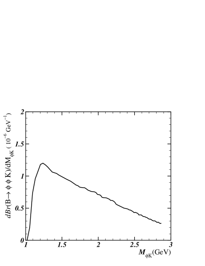
Figure 1: $B\to\phi K\gamma$ and $B\to\phi\phi K$ decay spectra in the $\phi K$ invariant mass.

After constraining the two-meson distribution amplitudes, we predict the $B\to\phi\phi K$ decay spectrum in the $\phi K$ invariant mass. For this mode, the amplitude ${\cal M}$ is written as

$${\cal M} = f_{\phi}V^{*}_{tb}V_{ts}\sum_{i=3}^{5}\Big{[}{\cal F}^{P(s)}_{Li}+\epsilon_{T}\cdot\epsilon_{3T}(\phi){\cal F}^{P(s)}_{Ti}\Big{]}\;,$$ (32)

$${\cal F}^{P(s)}_{Li} = 8\pi C_{F}m^{2}_{B}\int^{1}_{0}dx_{1}dz\frac{\Phi_{B}(x_{1})\Phi_{\parallel}(z,\zeta,w)}{x_{1}zm^{2}_{B}+P_{T}^{2}}$$ (33)

$$\times\Big{\{}\Big{[}(1+z)\Phi_{\parallel}(z,\zeta,w)+\sqrt{\eta}(1-2z)\Phi_{p}(z,\zeta,w)\Big{]}\frac{\alpha_{s}(t^{(1)}_{e})a_{i}^{(s)}(t^{(1)})}{zm^{2}_{B}+P_{T}^{2}}$$

$$+2\sqrt{\eta}\Phi_{p}(z,\zeta,w)\frac{\alpha_{s}(t^{(2)})a_{i}^{(s)}(t^{(2)}_{e})}{x_{1}m^{2}_{B}}\Big{\}}\;,$$

$${\cal F}^{P(s)}_{Ti} = 8r_{\phi}\pi C_{F}m^{2}_{B}\int^{1}_{0}dx_{1}dz\frac{\Phi_{B}(x_{1})}{x_{1}zm^{2}_{B}+P_{T}^{2}}$$ (34)

$$\times\Big{\{}\Big{[}\Phi_{T}(z,\zeta,w)+\Phi_{3}(z,\zeta,w)\sqrt{\zeta(1-\zeta)}+z\sqrt{\eta}\Phi_{v}(z,\zeta,w)\Big{]}\frac{\alpha_{s}(t^{(1)}_{e})a_{i}^{(s)}(t^{(1)})}{zm^{2}_{B}+P_{T}^{2}}$$

$$-\sqrt{\eta}\Phi_{v}(z,\zeta,w^{2})\frac{\alpha_{s}(t^{(2)})a_{i}^{(s)}(t^{(2)})}{x_{1}m^{2}_{B}}\Big{\}}\;,$$

where $\epsilon_{3T}(\phi)$ denote the polarization vectors of the $\phi$ meson emitted from the weak vertex. The definitions of the Wilson coefficients $a_{i}^{(q)}(t)$ are referred to CKL1 . For a similar reason, we have dropped all the $O(\eta)$ terms. Equations (27), (33) and (34) represent the amplitudes of the $B$ meson transition into a $VP$ meson pair associated with different effective operators. We display the predicted $B^{\pm}\to\phi\phi K^{\pm}$ decay spectrum in Fig. 1, which also exhibits a maximum at the $\phi K$ invariant mass around 1.3 GeV. Integrating the spectrum over $\eta$, we obtain the branching ratio without the resonant contribution in the $\phi\phi$ channel,

$$B(B^{\pm}\to\phi\phi K^{\pm})=(1.3^{+0.4}_{-0.3})\times 10^{-6}\;.$$ (35)

The uncertainty arises from the variation of the shape parameter $\omega_{B}$ of the $B$ meson distribution amplitude.

We have examined other sources of theoretical uncertainty. The correction to the branching ratios from the neglected $O(\eta)$ terms is about 10%. To investigate the uncertainty from different parametrization of meson distribution amplitudes, we have tried

$$\Phi^{\prime}_{B}(x)=N^{\prime}_{B}x(1-x)\exp\left[-\frac{1}{2}\left(\frac{xm_{B}}{\omega^{\prime}_{B}}\right)^{2}\right]\;.$$ (36)

First, the shape parameter $\omega^{\prime}_{B}=0.9$ GeV is determined from the fit to the value of the $B\to\pi$ transition form factor about 0.3. The model $\Phi^{\prime}_{B}(x)$ is then employed to fix the $\phi K$ two-meson distribution amplitudes from the data of the $B\to\phi K\gamma$ branching ratios. It is observed that the symmetric $z$ dependence in Eq. (19) should be modified into

$$z(1-z)\to z(1-z)[1+0.5(1-2z)]\;,$$ (37)

which is reasonable since the $\phi$ meson is heavier than the kaon. After going through the above procedure, we predict the $B\to\phi\phi K$ branching ratio using the distribution amplitudes in Eqs. (36) and (37), and find that the result increases only by 8%. We have also checked the sensitivity of our prediction to the parametrization of the time-like form factors. Obeying the normalization and the asymptotic behavior required by PQCD, the models with $(w-m_{\phi})^{2}$ [$(w-m_{\phi})^{3}$] being replaced by $w^{2}-m_{\phi}^{2}$ [$(w^{2}-m_{\phi}^{2})^{3/2}$] are also allowed. Adopting the $B$ meson distribution amplitude in Eq. (23), the $\tau\to\phi K\nu$ and $B\to\phi K\gamma$ data just imply a slight increase of the parameters $m_{\parallel}$ and $m_{T}$ to 3-4 GeV. Then we predict the $B\to\phi\phi K$ branching ratio using the new parametrization, which is enhanced only by 12%. The above investigations indicate that the PQCD predictions will be insensitive to the parametrization of meson distribution amplitudes, if the procedure of determining meson distribution amplitudes is followed.

Note that the $B^{\pm}\to\phi\phi K^{\pm}$ branching ratio has been measured to be $B(B^{\pm}\to\phi\phi K^{\pm})=(2.6^{+1.1}_{-0.9}\pm 0.3)\times 10^{-6}$ for a $\phi\phi$ invariant mass below 2.85 GeV Bel03 . We suggest that the decay spectrum in the $\phi K$ invariant mass should also be measured (only the spectrum in the $\phi\phi$ invariant mass was presented in Bel03 ), such that the dynamics of the $B\to VP$ transition can be explored. To derive the spectrum in the $\phi\phi$ invariant mass, we need to define the $VV$ two-meson distribution amplitudes, which will be discussed in the future.

We thank H.Y. Cheng and Y.Y. Charng for useful discussions. This work was supported in part by the National Science Council of R.O.C. under Grant No. NSC-92-2112-M-001-003 and No. NSC-92-2112-M-006-026.

References

(1) BELLE Coll., A. Garmash et al., Phys. Rev. D
65, 092005 (2002).
(2) BABAR Coll., B. Aubert et al., hep-ex/0206004.
(3) C.H. Chen and H-n. Li, Phys. Lett. B 561, 258
(2003).
(4) D. Muller et al., Fortschr. Physik. 42, 101 (1994);
M. Diehl, T. Gousset, B. Pire, and O. Teryaev, Phys. Rev. Lett.
81, 1782 (1998); M.V. Polyakov, Nucl. Phys. B555, 231
(1999).
(5) G.P. Lepage and S.J. Brodsky, Phys. Lett. B 87, 359
(1979); Phys. Rev. Lett. 43, 545 (1979); G.P. Lepage and S.
Brodsky, Phys. Rev. D 22, 2157 (1980).
(6) S.J. Brodsky, Y. Frishman and G.P. Lepage,
and C. Sachrajda, Phys. Lett. B 91, 239 (1980).
(7) A.V. Efremov and A.V. Radyushkin, Theor. Math. Phys.
42, 97 (1980); Phys. Lett. B 94, 245 (1980);
I.V. Musatov and A.V. Radyushkin, Phys. Rev. D 56, 2713 (1997).
(8) A. Duncan and A.H. Mueller, Phys. Lett. B 90, 159
(1980); Phys. Rev. D 21, 1636 (1980).
(9) V.L. Chernyak, A.R. Zhitnitsky, and V.G. Serbo,
JETP Lett. 26, 594 (1977).
(10) J. Botts and G. Sterman, Nucl. Phys. B225, 62 (1989);
H-n. Li and G. Sterman, Nucl. Phys. B381, 129 (1992).
(11) H-n. Li, Phys. Rev. D 64, 014019 (2001);
M. Nagashima and H-n. Li, hep-ph/0202127; Phys. Rev. D 67,
034001 (2003).
(12) Y.Y. Keum, H-n. Li, and A.I. Sanda,
AIP Conf. Proc. 618, 229 (2002); Y.Y. Keum and A.I. Sanda,
Phys. Rev. D 67, 054009 (2003).
(14) M. Beneke, G. Buchalla, M. Neubert, and C.T. Sachrajda,
Phys. Rev. Lett. 83, 1914 (1999);
Nucl. Phys. B606, 245 (2001).
(15) C.H. Chang and H-n. Li, Phys. Rev. D 55, 5577 (1997);
T.W. Yeh and H-n. Li, Phys. Rev. D 56, 1615 (1997).
(16) Y.Y. Keum, H-n. Li, and A.I. Sanda,
Phys. Lett. B 504, 6 (2001); Phys. Rev. D 63, 054008 (2001);
Y.Y. Keum and H-n. Li, Phys. Rev. D63, 074006 (2001).
(17) C.D. Lü, K. Ukai, and M.Z. Yang, Phys. Rev. D 63,
074009 (2001).
(18) H.Y. Cheng, H-n. Li, and K.C. Yang,
Phys. Rev. D 60, 094005 (1999).
(19) H-n. Li and H.L. Yu, Phys. Rev. Lett. 74, 4388 (1995);
Phys. Rev. D 53, 2480 (1996).
(20) H-n. Li, Phys. Rev. D 66, 094010 (2002);
H-n. Li and K. Ukai, Phys. Lett. B 555, 197 (2003).
(21) M. Bauer, B. Stech, M. Wirbel,
Z. Phys. C 29, 637 (1985); Z. Phys. C 34, 103
(1987).
(22) C.K. Chua, W.S. Hou, and S.Y. Tsai,
Phys. Rev. D66, 054004 (2002); W.S. Hou, S.Y. Shiau, and
S.Y. Tsai, Phys. Rev. D 67, 034012 (2003).
(23) B. Bajc, S. Fajfer, R.J. Oakes, T.N. Pham, and
S. Prelovšek, Phys. Lett. B 447, 313 (1999);
S. Fajfer, T.N. Pham, and A. Prapotnik, hep-ph/0401120.
(24) H.Y. Cheng and K.C. Yang, Phys. Rev. D 66,
054015 (2002); Phys. Rev. D 66, 094009 (2002).
(25) O. Leitner, X.H. Guo, and A.W. Thomas,
Eur. Phys. J. C31, 215 (2003).
(26) Z.T. Wei, hep-ph/0301174.
(27) BELLE Coll., H.C. Huang et al., Phys. Rev. Lett.
91, 241802 (2003).
(28) Particle Data Group, K. Hagiwara et al., Phys. Rev.
D 66, 010001 (2002).
(29) M. Maul, Eur. Phys. J. C 21, 115 (2001).
(30) M. Diehl, Th. Feldmann, P. Kroll, and C. Vogt,
Phys. Rev. D 61, 074029 (2000); M. Diehl, T. Gousset, and
B. Pire, Phys. Rev. D 62, 073014 (2000).
(31) P. Ball, V.M. Braun, Y. Koike, and K. Tanaka,
Nucl. Phys. B529, 323 (1998).
(32) V.M. Braun and I.E. Filyanov, Z Phys. C 48, 239
(1990); P. Ball, J. High Energy Phys. 01, 010 (1999).
(33) T. Huang, X.H. Wu, and M.Z. Zhou, hep-ph/0402100.
(34) T. Kurimoto, H-n. Li, and A.I.
Sanda, Phys. Rev. D 65, 014007 (2002); Phys. Rev. D 67, 054028 (2003).
(35) A. Khodjamirian and R. Ruckl, Phys. Rev. D 58, 054013
(1998).
(36) P. Ball, JHEP 09, 005 (1998); Z.
Phys. C 29, 637 (1985).
(37) A.G. Grozin and M. Neubert, Phys. Rev. D 55,
272 (1997); M. Beneke and T. Feldmann, Nucl. Phys. B592, 3
(2000).
(38) S. Descotes and C.T. Sachrajda, Nucl. Phys. B625,
239 (2002).
(39) H. Kawamura, J. Kodaira, C.F. Qiao, and K. Tanaka,
Phys. Lett. B 523, 111 (2001); Erratum-ibid. 536, 344
(2002).
(40) H-n. Li and H.S. Liao, hep-ph/0404050.
(41) B.O. Lange and M. Neubert, Phys. Rev. Lett. 91,
102001 (2003).