Nuclear parton distribution functions and their uncertainties

Abstract

We analyze experimental data of nuclear structure-function ratios $F_{2}^{A}/F_{2}^{A^{\prime}}$ and Drell-Yan cross section ratios for obtaining optimum parton distribution functions (PDFs) in nuclei. Then, uncertainties of the nuclear PDFs are estimated by the Hessian method. Valence-quark distributions are determined by the $F_{2}$ data at large $x$; however, the small-$x$ part is not obvious from the data. On the other hand, the antiquark distributions are determined well at $x\sim 0.01$ from the $F_{2}$ data and at $x\sim 0.1$ by the Drell-Yan data; however, the large-$x$ behavior is not clear. Gluon distributions cannot be fixed by the present data and they have large uncertainties in the whole $x$ region. Parametrization results are shown in comparison with the data. We provide a useful code for calculating nuclear PDFs at given $x$ and $Q^{2}$.

I Introduction

Parton distribution functions (PDFs) in the nucleon have been obtained by analyzing high-energy nucleon reaction data pdfs . Such an analysis is crucial for calculating precise cross sections for finding new physics phenomena. These investigations are valuable for clarifying internal hadron structure, and the studies ultimately lead to establishment of the nonperturbative aspect of quantum chromodynamics (QCD).

It is well known that nuclear parton distribution functions (NPDFs) are modified from those of the nucleon sumemc . It was first found by the European Muon Collaboration (EMC). Now, major features of the $x$-dependent modification became clear experimentally. Although a variety of data are not still available in comparison with the nucleonic case, the PDF parametrization could be done for the NPDFs ekrs ; saga01 ; fs03 . The first $\chi^{2}$ analysis for the NPDFs was done in Ref. saga01 by using a similar technique to the polarized PDF analysis of the Asymmetry Analysis Collaboration (AAC) aac00 . There are also related studies on nuclear shadowing recent-shadow . The word “shadowing” is used for nuclear modification at $x\lesssim 0.1$ throughout this paper.

These NPDF studies are valuable for describing high-energy nuclear scattering phenomena heavy . High-energy heavy-ion reactions have been investigated for finding a quark-gluon plasma signature. Because such a signature should be found in a modification of cross sections, the NPDFs should be exactly known. In addition, there is a strong demand from the neutrino community to have precise neutrino-nucleus, typically the oxygen nucleus, cross sections for investigating neutrino oscillation phenomena accurately nuint ; sakuda ; py . These necessities motivated us to investigate the NPDF parametrization.

In addition, it is interesting to find how well the NPDFs are determined. There have been studies of PDF uncertainties in the nucleon. It was investigated in the unpolarized PDFs pdf-error , and then the studies were extended to the polarized PDF uncertainties polpdf-error ; aac03 . Although error bands are shown for the NPDFs in Ref. saga01 , they are not based on a rigorous error analysis. Here, we calculate the NPDF uncertainties by using the Hessian method, which is a standard statistical procedure for estimating errors pdf-error ; polpdf-error ; aac03 .

The purpose of this paper is to report investigations after the publication in Ref. saga01 . In particular, the followings are added to the previous analysis: (1) Drell-Yan data are included in the data set. (2) HERMES data are also added. (3) Charm-quark distribution is included. (4) Uncertainties of the NPDFs are estimated by the Hessian method.

This paper consists of the following. In Sec. II, the $\chi^{2}$ analysis method, in particular the parametrization form and experimental data, is explained. Analysis results are shown in Sec. III and they are summarized in Sec. IV.

II Analysis method

We discuss the $\chi^{2}$ analysis method. First, the $x$ and $A$ dependence of the initial PDFs is explained, and comments are given on charm-quark distributions. Then, experimental data are introduced, and the uncertainty estimation method is explained.

II.1 Parametrization

The NPDFs are provided by a number of parameters at a fixed $Q^{2}$, which is denoted $Q_{0}^{2}$. The NPDFs could be directly expressed by a functional form with parameters, which are obtained by a $\chi^{2}$ analysis. However, experimental data are not sufficient for fixing detailed NPDFs. Therefore, it is more practical at this stage to parametrize nuclear modification rather than the NPDFs themselves. Namely, a NPDF is taken as the corresponding nucleonic PDF multiplied by a weight function $w_{i}$:

$$f_{i}^{A}(x,Q_{0}^{2})=w_{i}(x,A,Z)\,f_{i}(x,Q_{0}^{2}).$$ (1)

The nuclear modification part $w_{i}$ is obtained by a $\chi^{2}$ analysis. Here, $A$ is the mass number and $Z$ is the atomic number of a nucleus.

One of the essential points of the $\chi^{2}$ analysis is how to choose the $x$ and $A$ dependent functional form. Because nuclear modification mechanisms are different depending on the $x$ region, the $A$ dependence could be different in each $x$ region. If we would like to describe $w_{i}$ precisely, it could be a complicated function of mixed $x$ and $A$. However, instead of assuming a complicated functional form, we use a simple one at this stage. We leave such a complicated analysis for our future work. In Ref. saga01 , a simple overall $1/A^{1/3}$ dependence is assumed sd : $w_{i}=1+(1-1/A^{1/3})$($x$ dependent function). Here, we assume the same functional form. The weight function used for the following analysis is given by:

$$w_{i}(x,A,Z)=1+\left(1-\frac{1}{A^{\alpha}}\right)\frac{a_{i}(A,Z)+b_{i}x+c_{i}x^{2}+d_{i}x^{3}}{(1-x)^{\beta_{i}}},$$ (2)

where $i$ indicates the parton distribution type, and it is taken as $i=u_{v}$, $d_{v}$, $\bar{q}$, and $g$. Among these parameters, three parameters can be fixed by baryon-number, charge, and momentum conservations saga01 ; fsl . The motivation is explained for choosing this functional form in Ref. saga01 .

II.2 Charm-quark distributions

In the previous analysis, the flavor number is limited to three. However, charm-quark distributions are important for practical applications. For example, charmonium productions are used for searching a quark-gluon plasma signature in heavy-ion reactions. The charm distributions are also important in neutrino reactions py . Therefore, we add nuclear charm-quark distributions into the analysis.

At $Q^{2}=m_{c}^{2}$, where $m_{c}$ is the charm-quark mass, the running coupling constants for the flavor-number three and four should agree each other: $\alpha_{s}^{N_{f}=3}(m_{c}^{2})=\alpha_{s}^{N_{f}=4}(m_{c}^{2})$. In the leading order (LO), it leads to the relation between scale parameters: $\Lambda_{3}=\Lambda_{4}(m_{c}/\Lambda_{4})^{2/27}$. Since the initial distributions in Eq. (1) are provided at $Q^{2}$ which is smaller than $m_{c}^{2}$ in our analysis, optimized parameters for the charm distributions do not exist. The distributions appear simply as $Q^{2}$ evolution effects.

II.3 Experimental data

Table 1: Nuclear species, experiments, references, and the number of data points are listed for the used data with $Q^{2}\geq 1$ GeV².

nucleus	experiment	reference	# of data
($F_{2}^{A}/F_{2}^{D}$)
4He/D	SLAC-E139	slac94	18
	NMC-95	nmc95	17
Li/D	NMC-95	nmc95	17
Be/D	SLAC-E139	slac94	17
C/D	EMC-88	emc88	9
	EMC-90	emc90	5
	SLAC-E139	slac94	7
	NMC-95	nmc95	17
	FNAL-E665-95	e665-95	5
N/D	BCDMS-85	bcdms85	9
	HERMES-03	hermes03	153
Al/D	SLAC-E49	slac83B	18
	SLAC-E139	slac94	17
Ca/D	EMC-90	emc90	5
	NMC-95	nmc95	16
	SLAC-E139	slac94	7
	FNAL-E665-95	e665-95	5
Fe/D	SLAC-E87	slac83	14
	SLAC-E140	slac88	10
	SLAC-E139	slac94	23
	BCDMS-87	bcdms87	10
Cu/D	EMC-93	emc93	19
Kr/D	HERMES-03	hermes03	144
Ag/D	SLAC-E139	slac94	7
Sn/D	EMC-88	emc88	8
Xe/D	FNAL-E665-92	e665-92	5
Au/D	SLAC-E140	slac88	1
	SLAC-E139	slac94	18
Pb/D	FNAL-E665-95	e665-95	5
$F_{2}^{A}/F_{2}^{D}$ total			606
($F_{2}^{A}/F_{2}^{A^{\prime}}$)
Be/C	NMC-96	nmc96	15
Al/C	NMC-96	nmc96	15
Ca/C	NMC-95	nmc95	24
	NMC-96	nmc96	15
Fe/C	NMC-96	nmc96	15
Sn/C	NMC-96	nmc96snc	146
Pb/C	NMC-96	nmc96	15
C/Li	NMC-95	nmc95	24
Ca/Li	NMC-95	nmc95	24
$F_{2}^{A}/F_{2}^{A^{\prime}}$ total			293
($\sigma_{DY}^{pA}/\sigma_{DY}^{pA^{\prime}}$)
C/D	FNAL-E772-90	e772-90	9
Ca/D	FNAL-E772-90	e772-90	9
Fe/D	FNAL-E772-90	e772-90	9
W/D	FNAL-E772-90	e772-90	9
Fe/Be	FNAL-E866/NuSea-99	e866-99	8
W/Be	FNAL-E866/NuSea-99	e866-99	8
Drell-Yan total			52
total			951

In the previous version saga01 , the used experimental data are limited to the ratios $F_{2}^{A}/F_{2}^{D}$ where $D$ indicates the deuteron. The data are from European Muon Collaboration (EMC) emc88 ; emc90 ; emc93 , the SLAC-E49, E87, E139, and E140 Collaborations slac83 ; slac83B ; slac88 ; slac94 , the Bologna-CERN-Dubna-Munich-Saclay (BCDMS) Collaboration bcdms85 ; bcdms87 , the New Muon Collaboration (NMC) nmc95 , and the Fermilab-E665 Collaboration e665-92 ; e665-95 . These data are listed in the $F_{2}^{A}/F_{2}^{D}$ section of Table 1.

In addition to these data, we added HERMES data for the ratios $F_{2}^{A}/F_{2}^{D}$, where the nucleus $A$ is for nitrogen and krypton hermes03 . Furthermore, the ratios $F_{2}^{A}/F_{2}^{A^{\prime}}$ ($A^{\prime}\neq D$) were measured by the NMC nmc95 ; nmc96 ; nmc96snc , and these data are also added. The Drell-Yan data taken by the Fermilab-E772 e772-90 and E866/NuSea e866-99 collaborations are added into the data set for the $\chi^{2}$ analysis. In Refs. e772-90 ; e866-99 , $Q^{2}$ (dimuon mass) values are not listed. Therefore, we calculated the values in the following way peng . Relations between the dimuon mass and the target momentum fraction $x_{2}$ are listed in Ref. e772-92 . We interpolated these values to obtain the $Q^{2}$ information.

One may note that HERMES ³He data are not included into the data set. The data are not well reproduced by the present fit, so that the data produce a significantly large $\chi^{2}$ value. It comes from the fact that the ³He is a tightly bound nucleus which cannot be expressed by the simple $1-1/A^{\alpha}$ dependence. In order to reproduce such a nucleus, more complicated $A$ dependent function should be used for the analysis.

The number of data points is listed in Table 1. The data are for the nuclei: deuteron (D), helium-4 (⁴He), lithium (Li), beryllium (Be), carbon (C), nitrogen (N), aluminum (Al), calcium (Ca), iron (Fe), copper (Cu), krypton (Kr), silver (Ag), tin (Sn), xenon (Xe), tungsten (W), gold (Au), and lead (Pb). The numbers of the $F_{2}^{A}/F_{2}^{D}$, $F_{2}^{A}/F_{2}^{A^{\prime}}$ ($A^{\prime}\neq D$), and Drell-Yan data are 606, 293, and 52, respectively. The total number is 951.

Figure 1: (Color online) Kinematical range is shown by $x$ and $Q^{2}$ values of the used data.

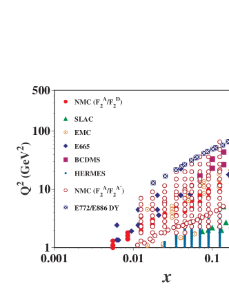
The kinematical range of the used data is shown in Fig. 1. The smallest $x$ value with $Q^{2}\geq$1 GeV² is 0.0055 at this stage, and it is rather limited in comparison with the proton data ($x_{min}\sim 10^{-4}$) at HERA. The SLAC data are taken in the large $x$, small $Q^{2}$ region, and the CERN-EMC, NMC, and Fermilab-E665 data are taken in the wide $x$ region from small $x$ to large $x$. The Drell-Yan data are in the large $Q^{2}$ region.

Table 2: Parameters obtained by the analysis. The parameters $a_{u_{v}}$, $a_{d_{v}}$, and $a_{g}$ are fixed by three conservations. Because they depend on nuclear species, they are explained separately in Appendix A.

distribution	$a$	$b$	$c$	$d$
$u_{v}^{A}$, $d_{v}^{A}$	fixed (Appendix)	2.894 $\pm$ 0.395	$-$9.390 $\pm$ 1.068	7.308 $\pm$ 0.866
$\bar{q}^{A}$	$-$0.3794 $\pm$ 0.0461	8.626 $\pm$ 1.551	$-$56.64 $\pm$ 11.84	94.11 $\pm$ 27.57
$g^{A}$	fixed (Appendix)	2.165 $\pm$ 3.126	0.000 (fixed)	1.349 $\pm$ 44.56

II.4 $\chi^{2}$ analysis

Nuclear modification of the PDFs is expressed by the weight functions $w_{i}$. We introduce four types by assuming the flavor symmetric antiquark distributions ($\bar{u}^{A}=\bar{d}^{A}=\bar{s}^{A}\equiv\bar{q}^{A}$) at $Q_{0}^{2}$:

$$u_{v}^{A}(x,Q_{0}^{2}) =w_{u_{v}}(x,A,Z)\,\frac{Zu_{v}(x,Q_{0}^{2})+Nd_{v}(x,Q_{0}^{2})}{A},$$

$$d_{v}^{A}(x,Q_{0}^{2}) =w_{d_{v}}(x,A,Z)\,\frac{Zd_{v}(x,Q_{0}^{2})+Nu_{v}(x,Q_{0}^{2})}{A},$$

$$\bar{q}^{A}(x,Q_{0}^{2}) =w_{\bar{q}}(x,A,Z)\,\bar{q}(x,Q_{0}^{2}),$$

$$g^{A}(x,Q_{0}^{2}) =w_{g}(x,A,Z)\,g(x,Q_{0}^{2}).$$ (3)

In the first two equations, the $Z$ terms indicate the proton contributions and the $N$ terms indicate the neutron ones if there were no nuclear modification and isospin symmetry could be applied. Although the antiquark distributions ($\bar{u}$, $\bar{d}$, $\bar{s}$) in the nucleon are different flavor3 , there is no clear data which indicates the difference in nuclei at this stage. Therefore, the flavor symmetric antiquark distributions are assumed. The initial scale is chosen $Q_{0}^{2}$=1 GeV². The MRST01-LO (Martin-Roberts-Stirling-Thorne, leading-order version of 2001) parametrization mrst01 is used for the PDFs, so that scale parameter $\Lambda$ and charm-quark mass $m_{c}$ are the MRST01 values in the following analysis.

Using these NPDFs, we calculate the structure-function ratios $F_{2}^{A}/F_{2}^{A^{\prime}}$ and the Drell-Yan cross section ratios $\sigma_{DY}^{pA}/\sigma_{DY}^{pA^{\prime}}$ in the leading order (LO) of $\alpha_{s}$. The NPDFs are given at $Q_{0}^{2}$ in Eq. (3), so that they are evolved to the experimental $Q^{2}$ points by the Dokshitzer-Gribov-Lipatov-Altarelli-Parisi (DGLAP) evolution equations in order to calculate these ratios. The total $\chi^{2}$ is defined by

$$\chi^{2}=\sum_{j}\frac{(R_{j}^{data}-R_{j}^{theo})^{2}}{(\sigma_{j}^{data})^{2}},$$ (4)

where $R_{j}$ indicates that the ratios, $F_{2}^{A}/F_{2}^{A^{\prime}}$ and $\sigma_{DY}^{pA}/\sigma_{DY}^{pA^{\prime}}$. The experimental errors are calculated from systematic and statistical errors by $(\sigma_{j}^{data})^{2}=(\sigma_{j}^{sys})^{2}+(\sigma_{j}^{stat})^{2}$. The optimization of the NPDFs is done by the CERN subroutine MINUIT minuit .

II.5 Uncertainty of nuclear PDFs

Because the situation of the NPDFs is not as good as the one of the PDFs in the nucleon, it is especially important to show the reliability of obtained NPDFs. The uncertainties are shown in the previous version saga01 ; however, they are simply estimated by shifting each parameter by the amount of the error. Of course, a standard error analysis is needed for the NPDFs by taking into account correlations among the parameter errors.

One of the popular ways is to use the Hessian method. In fact, it is used for the unpolarized PDF analysis of the nucleon pdf-error and also for the polarized PDFs polpdf-error ; aac03 . Because the method is discussed in Ref. aac03 , we explain only a brief outline.

The parameters of the initial NPDFs in Eq. (2) are denoted $\xi_{i}$ ($i$=1, 2, $\cdot\cdot\cdot$, $N$), where $N$ is the number of the parameters. The $\chi^{2}$ could be expanded around the minimum point $\hat{\xi}$:

$$\Delta\chi^{2}\equiv\chi^{2}(\hat{\xi}+\delta\xi)-\chi^{2}(\hat{\xi})=\sum_{i,j}H_{ij}\delta\xi_{i}\delta\xi_{j}\,,$$ (5)

where $H_{ij}$ is called Hessian. The details are discussed elsewhere for the uncertainty estimation of the PDFs by the Hessian method. For the detailed explanation, one may read Refs. pdf-error ; aac03 about $\Delta\chi^{2}$ and the Hessian. A confidence region is identified by providing the $\Delta\chi^{2}$ value, which is determined in the following way. The confidence level $P$ could be chosen as the one-$\sigma$-error range of the normal distribution ($P=0.6826$). For one parameter, $P=0.6826$ is obtained with $\Delta\chi^{2}$=1. However, a different value should be assigned for the $N$ degrees of freedom aac03 . For example, if there are nine parameters, the $\Delta\chi^{2}$ value is calculated as $\Delta\chi^{2}=10.427$.

The uncertainty of a NPDF $f^{A}(x,\hat{\xi})$ is calculated by the Hessian matrix, which is obtained by running the MINUIT subroutine, and derivatives of the distribution:

$$[\delta f^{A}(x)]^{2}=\Delta\chi^{2}\sum_{i,j}\left(\frac{\partial f^{A}(x,\hat{\xi})}{\partial\xi_{i}}\right)H_{ij}^{-1}\left(\frac{\partial f^{A}(x,\hat{\xi})}{\partial\xi_{j}}\right)\,.$$ (6)

The derivatives are calculated analytically at the initial scale $Q^{2}_{0}$, and then they are evolved to certain $Q^{2}$ by the DGLAP evolution equations.

III Results

Analysis results are discussed. First, optimized parameters are shown, and $\chi^{2}$ contributions from nuclear data sets are listed. Then, fit results are compared with experimental data. The actual NPDFs and their uncertainties are shown for some nuclei at $Q_{0}^{2}$.

III.1 Comparison with $x$-dependent data

Table 3: Each $\chi^{2}$ contribution.

nucleus	# of data	$\chi^{2}$
4He/D	35	56.0
Li/D	17	88.7
Be/D	17	44.1
C/D	43	130.8
N/D	162	136.9
Al/D	35	43.1
Ca/D	33	42.0
Fe/D	57	95.7
Cu/D	19	11.8
Kr/D	144	126.9
Ag/D	7	12.8
Sn/D	8	14.6
Xe/D	5	2.0
Au/D	19	61.6
Pb/D	5	5.6
$F_{2}^{A}/F_{2}^{D}$ total	606	872.8
Be/C	15	16.1
Al/C	15	6.1
Ca/C	39	36.5
Fe/C	15	10.3
Sn/C	146	257.3
Pb/C	15	25.3
C/Li	24	78.1
Ca/Li	24	107.7
$F_{2}^{A_{1}}/F_{2}^{A_{2}}$ total	293	537.4
C/D	9	9.8
Ca/D	9	7.2
Fe/D	9	8.1
W/D	9	18.3
Fe/Be	8	6.5
W/Be	8	29.6
Drell-Yan total	52	79.6
total	951	1489.8

Figure 2: (Color online) Comparison with experimental ratios $R=F_{2}^{A}/F_{2}^{D}$. The ordinate indicates the fractional differences between experimental data and theoretical values: $(R^{exp}-R^{theo})/R^{theo}$.

Figure 3: (Color online) Comparison with experimental data of $R=F_{2}^{A}/F_{2}^{C,Li}$. The ratios $(R^{exp}-R^{theo})/R^{theo}$ are shown.

Figure 4: (Color online) Comparison with Drell-Yan data of $R=\sigma_{DY}^{pA}/\sigma_{DY}^{pA^{\prime}}$. The ratios $(R^{exp}-R^{theo})/R^{theo}$ are shown.

Figure 5: (Color online) Parametrization results are compared with the data of $F_{2}$ ratios $F_{2}^{Ca}/F_{2}^{D}$ and Drell-Yan ratios $\sigma_{DY}^{pCa}/\sigma_{DY}^{pD}$. The theoretical curves and uncertainties are calculated at $Q^{2}$=5 GeV² for the $F_{2}$ ratios and at $Q^{2}$=50 GeV² for the Drell-Yan ratios.

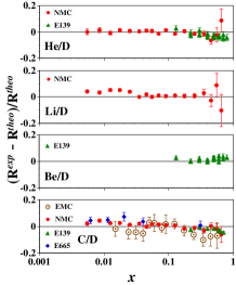
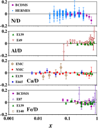
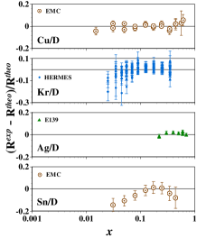
In the actual fit, the parameters for the Fermi-motion part are fixed at $\beta_{v}$=$\beta_{\bar{q}}$=$\beta_{g}$=0.1 because of the lack of large-$x$ data. The parameter $\alpha$ is also fixed at $\alpha=1/3$ saga01 for the $A$ dependence. The parameters obtained by the $\chi^{2}$ analysis are shown in Table 2. Three parameters are fixed by the charge, baryon-number, and momentum conservations, and they are chosen $a_{u_{v}}$, $a_{d_{v}}$, and $a_{g}$ in the analysis. Because these constants depend on nuclear species, they are listed separately in Appendix A. Another parameter $c_{g}$ is also fixed since the gluon parameters cannot be determined easily by the present data.

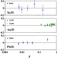
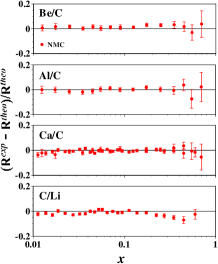
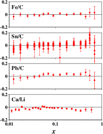
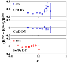
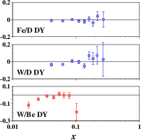
The $\chi^{2}$ analysis results are shown in comparison with the data. First, $\chi^{2}$ values are listed for each nuclear data set in Table 3. The total $\chi^{2}$ divided by the degree of freedom is 1.58. Comparison with the actual data is shown in Figs. 2, 3, and 4 for the $F_{2}^{A}/F_{2}^{D}$, $F_{2}^{A}/F_{2}^{C,Li}$, and Drell-Yan ($\sigma_{DY}^{pA}/\sigma_{DY}^{pA^{\prime}}$) data, respectively. These ratios are denoted $R^{exp}$ for the experimental data and $R^{theo}$ for the parametrization calculations. The deviation ratios $(R^{exp}-R^{theo})/R^{theo}$ are shown in these figures. The NPDFs are evolved to the experimental $Q^{2}$ points, then the ratios $(R^{exp}-R^{theo})/R^{theo}$ are calculated.

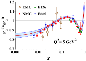
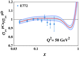
As examples, actual data are compared with the parametrization results in Fig. 5 for the ratios $F_{2}^{Ca}/F_{2}^{D}$ and $\sigma_{DY}^{pCa}/\sigma_{DY}^{pD}$. The shaded areas indicate the ranges of NPDF uncertainties, which are calculated at $Q^{2}$=5 GeV² for the $F_{2}$ ratios and at $Q^{2}$=50 GeV² for the Drell-Yan ratios. The experimental data are well reproduced by the parametrization, and the the data errors agree roughly with the uncertainty bands. We should note that the parametrization curves and the uncertainties are calculated at at $Q^{2}$=5 and 50 GeV², whereas the data are taken at various $Q^{2}$ points. In Fig. 5, the smallest-$x$ data at $x$=0.0062 for $F_{2}^{Ca}/F_{2}^{D}$ seems to deviate from the parametrization curve. However, the deviation comes simply from a $Q^{2}$ difference. In fact, if the theoretical ratio is estimated at the experimental $Q^{2}$ point, the data point agrees with the parametrization as shown in Fig. 2.

In general, the figures indicate a good fit to the data, which suggests that the $\chi^{2}$ analysis should be successful. However, there are some deviations as indicated in the table and figures. The $\chi^{2}$ contributions are large from small nuclei. For example, the $Li/D$ ratios have the $\chi^{2}$ value 88.7 for only 17 data points. In fact, the $Li/D$ ratios in the region $x\sim 0.01$ deviate from the theoretical curve in Fig. 2. The $Li/D$ ratios are measured with small errors so that they produce large $\chi^{2}$ values. However, if we wish to reproduce the $Li/D$ ratios, the ${}^{4}He/D$ and $Be/D$ ratios cannot be well explained. This is why the MINUIT subroutine produced the optimum point although theoretical calculations deviate from the experimental $Li/D$ ratios. We also notice that the $Sn/C$, $C/Li$, and $Ca/Li$ ratios are not well reproduced in the region $x<0.04$. On the other hand, the figures indicate that medium- and large-size nuclei are well explained by the parametrization model.

The Drell-Yan data are taken mainly in the range $0.02<x<0.2$ as shown in Fig. 4. The Drell-Yan cross section ratio $\sigma_{DY}^{pA}/\sigma_{DY}^{pA^{\prime}}$ is almost identical to the antiquark ratio $\bar{q}^{A}(x_{2})/\bar{q}^{A^{\prime}}(x_{2})$ in the $x$ region, $x<0.1$. Therefore, the Drell-Yan data are especially valuable for determining the antiquark modification in the $x$ region, $x\sim 0.1$. In the smaller $x$ region, the antiquark shadowing is fixed by the $F_{2}$ data in any case. Except for the $W/Be$ Drell-Yan ratios in the region $x\sim 0.02$, the data are well explained by the parametrization. From the constraints of these Drell-Yan cross sections, $F_{2}$ shadowing, and momentum conservation, the antiquark distributions are relatively well determined in the region $0.006<x<0.1$. However, the behavior of the medium- and large-$x$ regions is not obvious.

III.2 Comparison with $Q^{2}$-dependent data

Figure 6: (Color online) $Q^{2}$ dependence of $F_{2}^{Kr}/F_{2}^{D}$. The curves indicate parametrization results.

Figure 7: (Color online) $Q^{2}$ dependence of $F_{2}^{N}/F_{2}^{D}$.

Figure 8: (Color online) $Q^{2}$ dependence of $F_{2}^{Sn}/F_{2}^{C}$.

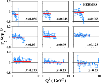
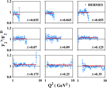
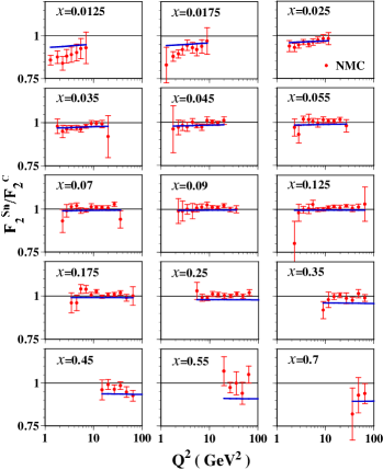
The analysis results are compared with $Q^{2}$ dependent data in Figs. 6, 7, and 8 for the ratios, $F_{2}^{Kr}/F_{2}^{D}$, $F_{2}^{N}/F_{2}^{D}$, and $F_{2}^{Sn}/F_{2}^{C}$, respectively. The fit results are shown by the curves in these figures. The data are well reproduced by the fit except for the $Sn/C$ ratios at small and medium $x$. The tin shadowing is underestimated in comparison with the carbon shadowing as indicated in the previous subsection. However, we notice that the experimental data are not “consistent” in the sense that the $F_{2}^{Kr}/F_{2}^{D}$ and $F_{2}^{N}/F_{2}^{D}$ ratios tend to decrease at $x$=0.035 and 0.045 with increasing $Q^{2}$, whereas the $F_{2}^{Sn}/F_{2}^{C}$ ratio increases. Obviously, more detailed experimental investigations should be done for clarifying the $Q^{2}$ dependence. It is especially important for fixing the gluon distributions in nuclei. The $Q^{2}$ dependence is related partially to the nuclear gluon distributions through the $Q^{2}$ evolution equations. If the experimental $Q^{2}$ dependence becomes clear, we should be able to pin down the nuclear gluon modification.

III.3 Optimum parton distribution functions

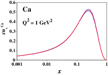
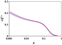
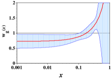
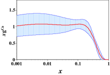
We show the nuclear parton distribution functions obtained by the $\chi^{2}$ analysis. As a typical medium-sized nucleus, the calcium is selected for showing the distributions. Because it is an isoscalar nucleus, the $u_{v}^{A}$ and $d_{v}^{A}$ are identical. Therefore, $u_{v}^{Ca}$ (=$d_{v}^{Ca}$), $\bar{q}^{\,Ca}$, and $g^{Ca}$ and their weight functions are shown in Fig. 9 at $Q_{0}^{2}$.

The valence-quark modification $w_{u_{v}}$ is precisely determined by the data in the medium- and large-$x$ regions. However, the uncertainty band becomes larger in the region $x<0.03$ although it is constrained somewhat by the charge and baryon-number conservations. Obviously, we should wait for NuMI (Neutrinos at the Main Injector) numi and neutrino-factory nufact03 projects for clarifying the valence-quark shadowing by the structure function $F_{3}$. Although the uncertainties of the nuclear modification $w_{u_{v}}^{Ca}$ are relatively large at $x<0.03$, it is not so obvious in the valence-quark distribution ($xu_{v}^{Ca}$), as shown on the right-hand side of Fig. 9, because the distribution is small in the small-$x$ region.

Figure 9: (Color online) The weight functions and the nuclear parton distribution functions are shown for the calcium nucleus at $Q_{0}^{2}$. The uncertainties are shown by the bands.

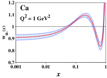
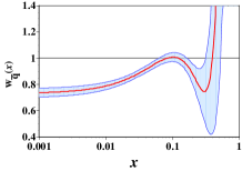
We should mention the possibility that the uncertainties could be underestimated because we fixed some parameters such as $\alpha$ and $\beta$ in the analysis. In addition, there should be uncertainties from the assumed functional form. These additional factors will be investigated in future. In this respect, it is certainly worth while investigating the $F_{3}$ shadowing at future neutrino facilities numi ; nufact03 in spite of the analysis result for the valence-quark shadowing in Fig. 9.

The uncertainties of the antiquark modification $w_{\bar{q}}^{Ca}$ are small in the region $x<0.1$ because it is fixed by the $F_{2}$ and Drell-Yan data. However, it has large uncertainties in the $x$ region, $x>0.2$. The antiquark distribution $x\bar{q}^{\,Ca}$ itself is small at $x>0.2$, so that it becomes difficult to take accurate data for the nuclear modification. In order to determine the distribution in this region, we need another Drell-Yan experiment which is intended especially for large-$x$ physics dy-large-x .

Figure 10: (Color online) The weight functions are shown for the nuclei, ⁴He, Ca, and Au, at $Q_{0}^{2}$.

The gluon distribution is especially difficult to be determined by the present data. It is clearly shown in Fig. 9 that the modification $w_{g}^{Ca}$ and the distribution $xg^{Ca}$ have large uncertainties. As explained in the previous subsection, the nuclear $Q^{2}$ dependence is not clear from the data. This fact makes it difficult to fix the nuclear gluon distributions. However, we notice that the gluon distribution seems to be shadowed although the uncertainties are large at $x<0.1$.

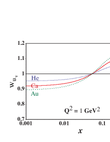
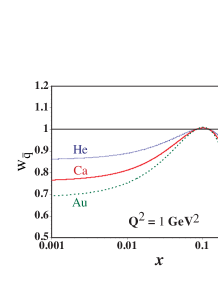
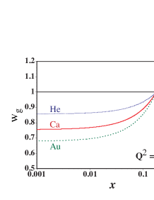
We notice that the functional form of the gluon weight function $w_{g}$ is different from those of the valence-quark and antiquark functions, $w_{v}$ and $w_{\bar{q}}$. A similar functional form was also tested in the analysis. We provided a weight function $w_{g}$, which has the same functional form with $w_{\bar{q}}$, as the initial one for the $\chi^{2}$ analysis without fixing the parameter $c_{g}$. However, the analysis ended up with gluon distributions which are similar to the one in Fig. 9. It is simply because of the lack of data which are sensitive to the gluon distributions. It is the reason why we decided to fix the parameter $c_{g}$ in the current analysis. The gluon distributions play an important role in many aspects of high-energy heavy-ion collisions, so that they should be determined by future experimental data. For example, the eRHIC project erhic could be a promising one for determining the nuclear PDFs at small $x$. In order to illustrate the nuclear dependence of the PDFs, we show the weight functions for the nuclei, ⁴He, Ca, and Au, in Fig. 10

For general users, a computer code is available on the web site nucl-lib for calculating the parton distribution functions for nuclei at given $x$ and $Q^{2}$. The details are explained in Appendix B.

IV Summary

The nuclear parton distribution functions and their uncertainties are determined by analyzing the experimental data of $F_{2}$ and Drell-Yan data. The uncertainties are estimated by the Hessian method. The valence-quark distributions are well determined except for the region $x<0.03$. The antiquark distributions have small uncertainties at $x<0.1$; however, they cannot be fixed in the region, $x>0.2$. The gluon distributions have large uncertainties in the whole-$x$ region. Obviously, we need much accurate scaling violation data or other ones for fixing the gluon distributions in nuclei.

Appendix A Nuclear dependent parameters

In Table 2, the constants $a_{u_{v}}$, $a_{d_{v}}$, and $a_{\bar{q}}$ are not listed. These constants are fixed by the three conservation equations, so that they depend on the mass number $A$ and the atomic number $Z$. For practical usage, we express these constants by eight integral values $I_{1-8}$ as explained in Ref. saga01 :

$$a_{u_{v}}(A,Z) =-\frac{ZI_{1}+(A-Z)I_{2}}{ZI_{3}+(A-Z)I_{4}},$$

$$a_{d_{v}}(A,Z) =-\frac{ZI_{2}+(A-Z)I_{1}}{ZI_{4}+(A-Z)I_{3}},$$

$$a_{g}(A,Z) =-\frac{1}{I_{8}}\,\bigg{[}\,a_{u_{v}}(A,Z)\left\{\frac{Z}{A}I_{5}+\left(1-\frac{Z}{A}\right)I_{6}\right\}$$

$$\!\!\!\!\!\!\!+a_{d_{v}}(A,Z)\left\{\frac{Z}{A}I_{6}+\left(1-\frac{Z}{A}\right)I_{5}\right\}+I_{7}\,\bigg{]}.$$ (1)

Values of the integrals are listed in Table 4 from the current analysis. Using these values together with Eq. (1), one could calculate the constants $a_{u_{v}}$, $a_{d_{v}}$, and $a_{\bar{q}}$ for any nucleus. Then, it is possible to express the nuclear parton distribution functions analytically at $Q_{0}^{2}$ for a given nucleus together with the MRST01 distributions mrst01 in the nucleon.

Table 4: Values of the eight integrals.

Integral	Value	Integral	Value
$I_{1}$	0.2611	$I_{5}$	0.3445
$I_{2}$	0.1313	$I_{6}$	0.1345
$I_{3}$	2.018	$I_{7}$	0.2162
$I_{4}$	1.016	$I_{8}$	0.3969

Appendix B Practical code for calculating nuclear PDFs

One could calculate nuclear PDFs by using the information provided in Appendix A and in Table 2. However, the distributions should be evolved if one wish to obtain them at different $Q^{2}$. For those who are not familiar with such $Q^{2}$ evolution, we prepared a practical code for calculating the nuclear PDFs at given $x$ and $Q^{2}$. The code could be obtained from the web site in Ref. nucl-lib .

Instructions for using the code are provided in the package. Only restrictions are the kinematical ranges, $10^{-9}\leq x\leq 1$, and 1 GeV${}^{2}\leq Q^{2}\leq 10^{8}$ GeV². The largest nucleus in the analysis is the lead, so that it is suitable to use the code within the range $A\leq 208$. However, variations of the NPDFs are rather small from $A=208$ to the nuclear matter, one could possibly use the code also for large nuclei with $A>208$. In the NPDF library, we provide the distributions at very small $x$ as small as $10^{-9}$ for those who use them in integrating the distributions over the wide range of $x$. However, one should be careful that the distributions are not reliable in the region $x<0.006$, where no experimental data exists. Furthermore, there is a possibility that higher-twist effects could alter the results in the small-$x$ region.

The analysis was made in the region, $Q^{2}\geq$1 GeV², where the perturbative QCD is considered to be applicable. The obtained NPDFs can be used for high-energy nuclear reactions with $Q^{2}\geq$1 GeV². However, there are data which are slightly below this region. For example, many long-baseline neutrino data are taken in the smaller $Q^{2}$ region. A useful parametrization was proposed to describe the cross section from the deep inelastic region to the resonance one by02 . We could possibly make a similar analysis in future for describing lepton-nucleus cross sections also in the resonance region.

References

- (1) http://durpdg.dur.ac.uk/hepdata/pdf.html.
- (2) For a summary, see D. F. Geesaman, K. Saito, and A. W. Thomas, Ann. Rev. Nucl. Part. Sci. 45, 337 (1995).
- (3) K. J. Eskola, V. J. Kolhinen, and P. V. Ruuskanen, Nucl. Phys. B535, 351 (1998); K. J. Eskola, V. J. Kolhinen, and C. A. Salgado, Eur. Phys. J. C9, 61 (1999).
- (4) M. Hirai, S. Kumano, and M. Miyama, Phys. Rev. D64, 034003 (2001).
- (5) D. de Florian and R. Sassot, hep-ph/0311227.
- (6) Y. Goto et al. (Asymmetry Analysis Collaboration (AAC)), Phys. Rev. D62, 034017 (2000).
- (7) N. Armesto and C. A. Salgado, Phys. Lett. B520, 124 (2001); B. Z. Kopeliovich and A. V. Tarasov, Nucl. Phys. A710, 180 (2002); L. Frankfurt, V. Guzey, and M. Strikman, hep-ph/0303022; N. Armesto et al., Eur. Phys. J. C29, 531 (2003).
- (8) Shi-yuan Li and Xin-Nian Wang, Phys. Lett. B527, 85 (2002); X. Zhang and G. Fai, Phys. Rev. C65, 064901 (2002); A. Chamblin and G. C. Nayak, Phys. Rev. D66, 091901 (2002); E. Iancu and R. Venugopalan, hep-ph/0303204; P. Levai et al., nucl-th/0306019; A. Dainese, nucl-ex/0311004.
- (9) http://nuint.ps.uci.edu/; http://neutrino.kek.jp/nuint01/.
- (10) M. Sakuda, Nucl. Phys. B112, 109 (2002).
- (11) E. A. Paschos and J. Y. Yu, Phys. Rev. D65, 033002 (2002).
- (12) CTEQ collaboration, J. Pumplin et al., Phys. Rev. D65, 014013 (2001); JHEP 0207, 012 (2002); M. Botje, J. Phys. G28, 779 (2002); ZEUS collaboration, S. Chekanov et al., Phys. Rev. D67, 012007 (2003); A. D. Martin, R. G. Roberts, W. J. Stirling, and R. S. Thorne, Eur. Phys. J. C28, 455 (2003), hep-ph/0308087.
- (13) E. Leader, A. V. Sidorov, and D. B. Stamenov, Eur. Phys. J C23, 479 (2002); J. Blümlein and H. Böttcher, Nucl. Phys. B636, 225 (2002).
- (14) M. Hirai, S. Kumano, and N. Saito (AAC), Phys. Rev. D69, 054021 (2004); http://hs.phys.saga-u.ac.jp/aac.html.
- (15) I. Sick and D. Day, Phys. Lett. B274, 16 (1992).
- (16) L. L. Frankfurt, M. I. Strikman, and S. Liuti, Phys. Rev. Lett. 65, 1725 (1990).
- (17) J. Ashman et al. (European Muon Collaboration (EMC)), Phys. Lett. B202, 603 (1988).
- (18) M. Arneodo et al. (EMC), Nucl. Phys. B333, 1 (1990).
- (19) J. Ashman et al. (EMC), Z. Phys. C57, 211 (1993).
- (20) A. Bodek et al. (SLAC-E87 Collaboration), Phys. Rev. Lett. 50, 1431 (1983).
- (21) A. Bodek et al. (SLAC-E49), Phys. Rev. Lett. 51, 534 (1983).
- (22) S. Dasu et al. (SLAC-E140), Phys. Rev. Lett. 60, 2591 (1988).
- (23) J. Gomez et al. (SLAC-E139), Phys. Rev. D49, 4348 (1994).
- (24) G. Bari et al. (BCDMS Collaboration), Phys. Lett. 163B, 282 (1985).
- (25) A. C. Benvenuti et al. (BCDMS), Phys. Lett. B189, 483 (1987).
- (26) P. Amaudruz et al. (New Muon Collaboration (NMC)), Nucl. Phys. B441, 3 (1995); M. Arneodo et al. (NMC), Nucl. Phys. B441, 12 (1995).
- (27) M. R. Adams et al. (FNAL-E665 Collaboration), Phys. Rev. Lett. 68, 3266 (1992).
- (28) M. R. Adams et al. (E665), Z. Phys. C67, 403 (1995).
- (29) A. Airapetian et al. (HERMES Collaboration), Phys. Lett. B567, 339 (2003).
- (30) M. Arneodo et al. (NMC), Nucl. Phys. B481, 3 (1996).
- (31) M. Arneodo et al. (NMC), Nucl. Phys. B481, 23 (1996).
- (32) D. M. Alde et al. (FNAL-E772 Collaboration), Phys. Rev. Lett. 64, 2479 (1990).
- (33) M. A. Vasiliev et al. (FNAL-E866/NuSea Collaboration), Phys. Rev. Lett. 83, 2304 (1999).
- (34) J.-C. Peng and M. A. Vasiliev, personal communications.
- (35) P. L. McGaughey et al. (FNAL-E772), Phys. Rev. Lett. 69, 1726 (1992).
- (36) S. Kumano, Phys. Rep. 303, 183 (1998); G. T. Garvey and J.-C. Peng, Prog. Part. Nucl. Phys. 47, 203 (2001).
- (37) A. D. Martin, R. G. Roberts, W. J. Stirling, and R. S. Thorne, Phys. Lett. B531, 216 (2002).
-
(38)
F. James, CERN Program Library Long Writeup D506. See
http://wwwasdoc.web.cern.ch
/wwwasdoc/minuit/minmain.html. - (39) J. G. Morfin, J. Phys. G29, 1935 (2003); S. A. Kulagin, hep-ph/9812532.
- (40) S. Kumano, hep-ph/0310166, to be published in AIP proceedings of 5th International Workshop on Neutrino Factories and Superbeams, June 5-11, 2003, Columbia University, New York, USA.
- (41) The P906 Collaboration, proposal for Drell-Yan measurements at the FNAL Main Injector (1999). J. C. Peng, in KEK proceedings 2000-19, Workshop on Di-lepton Experiments at the 50-GeV PS, edited by J. Chiba and S. Sawada (2000).
- (42) http://quark.phy.bnl.gov/~ raju/eRHIC.html.
- (43) Nuclear parton-distribution subroutines could be obtained at the web site: http://hs.phys.saga-u.ac.jp/nuclp.html.
- (44) A. Bodek and U. K. Yang, Nucl. Phys. B112, 70 (2002).