Electroweak baryogenesis and primordial hypermagnetic fields

The origin of the matter-antimatter asymmetry of the universe remains one of the outstanding questions yet to be answered by modern cosmology and also one of only a handful of problems where the need of a larger number of degrees of freedom than those contained in the standard model (SM) is better illustrated. An appealing scenario for the generation of baryon number is the electroweak phase transition that took place when the temperature of the universe was about 100 GeV. Though in the minimal version of the SM, and without considering the interaction of the SM particles with additional degrees of freedom, this scenario has been ruled out given the current bounds for the Higgs mass, this still remains an open possibility in supersymmetric extensions of the SM. In recent years it has also been realized that large scale magnetic fields could be of primordial origin. A natural question is what effect, if any, these fields could have played during the electroweak phase transition in connection to the generation of baryon number. Prior to the electroweak symmetry breaking, the magnetic modes able to propagate for large distances belonged to the $U(1)$ group of hypercharge and hence receive the name of hypermagnetic fields. In this contribution, we summarize recent work aimed to explore the effects that these fields could have introduced during a first order electroweak phase transition. In particular, we show how these fields induce a CP asymmetric scattering of fermions off the true vacuum bubbles nucleated during the phase transition. The segregated axial charge acts as a seed for the generation of baryon number. We conclude by mentioning possible research venues to further explore the effects of large scale magnetic fields for the generation of the baryon asymmetry.

1 Introduction

The standard model (SM) of electroweak interactions meets all the requirements –commonly referred to as Sakharov conditions Sakharov – to generate a baryon asymmetry during the electroweak phase transition (EWPT), provided that this last be of first order. However, it is also well known that neither the amount of CP violation within the minimal SM nor the strength of the EWPT are enough to generate a sizable baryon number Gavela ; Kajantie . Supersymmetric extensions of the SM, with a richer particle content, contain new sources of CP violation CKN . They also allow a stronger first order phase transition Carena . In spite of these improvements with respect to the SM, the minimal supersymmetric model (MSSM) is severely constrained from experimental bounds on the chargino properties Cline leaving only a small corner of parameter space for the MSSM as a viable candidate for baryogenesis. Further possibilities to accommodate an explanation for the generation of baryon number during the EWPT include non-minimal supersymmetric models which, nonetheless, all share the unappealing feature of containing an even larger set of parameters than the already extensive number contained in the MSSM.

Though it might appear tempting to abandon the idea of electroweak baryogenesis (EWB) given the above difficulties, in recent years this possibility has been revisited due to the observation that magnetic fields are able to generate a stronger first order EWPT Giovannini ; Elmfors ; Giovannini2 . The situation is similar to what happens to a type I superconductor where an external magnetic field modifies the nature of the superconducting phase transition, changing it from second to first order due to the Meissner effect.

In spite of this observation, it has also been realized that the sphaleron bound becomes more restrictive due to the interaction between the sphaleron’s magnetic dipole moment and the external field Comelli . Nevertheless, these arguments are either classical or resort to perturbation theory to lowest order. However, in the absence of magnetic fields, it is well known that the phase transition picture is influenced by non-perturbative effects cast in terms of the resummation of certain classes of diagrams Carrington and it might also be expected that the same is true in the presence of magnetic fields. The situation with regards to the strength of the phase transition in the presence of magnetic fields is thus far from being settled and requires further research.

However, the influence on the magnetic fields on the enhancement of CP violation has received much less attention. In a series of recent papers Ayala1 ; Ayala2 ; Ayala3 , it has been shown that the external field is able to produce an axially asymmetric scattering of fermions off first order phase transition bubbles during the EWPT. This CP violating reflection is due to the chiral nature of the couplings of right- and left-handed modes with the external field in the symmetric phase . This mechanism produces an axial charge segregation which can then be transported in the symmetric phase where sphaleron induced transitions can convert it into baryon number Nelson . The main purpose of our work is the description of the mechanism for the generation of this axial charge segregation.

As was briefly presented in this introduction, the process of baryogenesis involves several physical ingredients which all deserve to be addressed in order to cover the entire topic; here we will concentrate on those aspects related to hypermagnetic fields, which are also one of the most recent and less explored parts of this field. For other aspects on the subject, we refer the reader to recent reviews Trodden ; Riotto ; Rubakov .

The work is organized as follows: in Sec. 2 we present the basic framework of electroweak baryogenesis. Sec. 3 is devoted to generalities of hypermagnetic fields and phase transitions. In Sec. 4 we summarize the current ideas for the origin of large scale magnetic fields as well as the experimental bounds on their strength set by different observations. In Sec. 5 we describe the mechanism whereby the asymmetric reflection of fermions off first order EWPT bubbles in the presence of external magnetic fields leads to an axial charge segregation that can then be converted into baryon number in the symmetric phase. Finally, in Sec. 6 we summarize and give a brief account of some possible research venues to further explore the influence of primordial magnetic fields in the generation of the baryon asymmetry of the universe.

2 Electroweak baryogenesis

2.1 Baryogenesis

The theory of baryogenesis is an intent to explain the existence of matter in the Universe. As Cohen, Kaplan and Nelson CKN put it: why is there something rather than nothing?

From the point of view of elementary particle physics, there is a symmetry between particles and antiparticles which suggests that there should be an overall balance between the amount of matter and antimatter in the universe. However the observed universe is composed almost entirely of matter, with no traces of present or primordial antimatter (see. e.g. Kolb pp 158–159, or Stecker for a recent review). On the other hand, from the cosmological approach, there is also some evidence that some ingredients are missing. In the hot early epoch of the universe evolution, one expects to have particles and antiparticles in thermal equilibrium with radiation; particle/antiparticle pairs would then annihilate each other until their annihilation rate becomes smaller than the rate of expansion of the universe. The remaining density of all the species can thus be estimated and it comes to be only a very small fraction of the closure density of the universe. In this way, if we do not wish to postulate that the universe was just born with ad hoc asymmetric initial conditions, we must find a mechanism to generate a net baryon number ($B=n_{b}-n_{\bar{b}}$).

In 1966, Sakharov Sakharov laid out the conditions for the development of a net excess of baryons over antibaryons: (1) Existence of interactions that violate baryon number; (2) C and CP violation and (3) departure from thermal equilibrium. (The implications of each one of these criteria is discussed in many places, see e.g. Ref. Trodden ).

It must be stressed however that some scenarios (possibly exotic) have been recently proposed where one of these conditions is not achieved (see e.g. Ref. Dolgov and references therein).

It is important to notice that a successful model for baryon generation has to put together two ingredients:

1) the generation of a baryon asymmetry

2) its preservation

In the following subsection, we will review the necessary conditions for both situations in the framework of EWB.

2.2 Electroweak baryogenesis

Sakharov conditions in the standard model

The sphaleron (the name is based on the classical greek adjective meaning “ready to fall”) Klink is an static and unstable solution of the field equations of the EW model, corresponding to the top of the energy barrier between two topologically distinct vacua. Transitions between these vacua are associated with the violation of baryon (B) and lepton number (L) 'tHooft , in the combination B + L, with leptons and baryons produced with the same rate (i.e. B - L conservation). For this reason, they can either induce baryogenesis, or be a mechanism for washing out the previously created baryon asymmetry. It is therefore important to define the epoch at which the sphaleron transitions fall out of thermal equilibrium.

As we mentioned, C and CP violation are present in the SM but are too tiny to be at the origin of the present baryon asymmetry Gavela ; Benreu . The generation of a sizable CP violation in the SM is the central part of this work and we will return to it later.

For the out of equilibrium requirement, we rely on the phase transition (PT). This is the only possible source of departure from thermal equilibrium since, at the electroweak scale, the rate of expansion of the universe is small compared to the rate of baryon number violating processes. But the PT is efficient in producing out-of-equilibrium conditions only if it is strongly first order Kuzmin , i.e. if the Higgs field –which is the order parameter in this case– undergoes a discontinuous change. In effect, in a first order PT, the conversion from one phase to another happens through nucleation and propagation of the true vacuum bubbles. The region separating both phases is called the wall. As the bubble wall sweeps a region in space, the order parameter changes rapidly, leading to a departure from thermal equilibrium.

Preservation of the baryon asymmetry

In order to freeze out the produced baryon number, the rate of fermion number non conservation in the broken phase, at temperatures below the bubble nucleation temperature, must be smaller than the rate of expansion of the universe.

The rate, per unit volume, of baryon number violating events, depends at low temperatures $T<T_{c}$ (more precisely for $M_{W}<<T<<M_{W}/\alpha_{W}$) on the sphaleron energy:

$$\Gamma=\mu\left(\frac{M_{W}}{\alpha_{W}T}\right)^{3}M_{W}^{4}\exp\left(\frac{E_{\mbox{\tiny{sph}}}(T)}{T}\right)\,,$$ (1)

with $\mu$ a dimensionless constant and $E_{\mbox{\tiny{sph}}}\sim M_{W}(T)/\alpha_{W}$ ($\alpha_{W}=g^{2}/4\pi$, with $g$ the $SU(2)_{L}$ gauge coupling). Comparing this rate with the rate of expansion of the universe $H\sim g_{*}^{1/2}T^{2}/m_{Pl}$ Kolb pp 60–65 ($g_{*}$ is the effective number of degrees of freedom and $m_{Pl}$ is the Planck mass), the following bound is found Shap1 :

$$E_{\mbox{\tiny{sph}}}(T_{\mbox{\tiny{nucl}}})/T_{\mbox{\tiny{nucl}}}>A\ \ ;\ \ A\simeq 35-45\,.$$ (2)

Here, we assume that the major wash-out is achieved near the nucleation epoch and we therefore consider only the nucleation temperature ($T_{\mbox{\tiny{nucl}}}$).

In principle, this condition can be translated to a bound on the order parameter of the PT, or on the Higgs mass Kajantie . However, there are a number of approximations and nontrivial steps involved in this procedure. The condition (2) is on the sphaleron energy at the temperature of bubble nucleation and it has to be related to the vacuum expectation value of the Higgs field (vev), at the critical temperature ($T_{c}$). These two temperatures are not exactly the same since, though the quantum tunneling phenomenon starts at $T_{c}$, initially the bubbles are not large enough for their volume energy to overcome the surface tension and they shrink. We have to wait for a lower temperature $T_{\mbox{\tiny{nucl}}}$, when bubbles are large enough to grow. Besides, $M_{H}$ is assumed to be equal to $M_{W}$ and there are a number of poorly known prefactors involved. In spite of these difficulties, a condition to avoid the sphaleron erasure is found and at present generally accepted:

$$(\phi/T)_{min}\simeq 1.0-1.5\,.$$ (3)

This bound represents a condition on the order of the PT, requiring a remarkable jump in the Higgs field.

On another hand, the order of the EWPT depends on the mass of all the particles of the theory (the $SU(2)_{L}\times U(1)_{Y}$ SM) and in particular on the Higgs boson mass M_H, which is at present not known. We only have constraints on it: the current lower bound on the Higgs mass from LEP LEP is: $m_{H}\mathrel{\mathchoice{\lower 0.5pt\vbox{\halign{$\mathnew\displaystyle\hfil#\hfil$\cr>\crcr\sim\crcr}}}{\lower 0.5pt\vbox{\halign{$\mathnew\textstyle\hfil#\hfil$\cr>\crcr\sim\crcr}}}{\lower 0.5pt\vbox{\halign{$\mathnew\scriptstyle\hfil#\hfil$\cr>\crcr\sim\crcr}}}{\lower 0.5pt\vbox{\halign{$\mathnew\scriptscriptstyle\hfil#\hfil$\cr>\crcr\sim\crcr}}}}114$ GeV.

The effective potential for the Higgs field, at finite temperature, can be written, including the radiative corrections from all the known SM particles:

$$V_{\mbox{\tiny{eff}}}\simeq-\frac{1}{2}(\mu^{2}-\alpha T^{2})\phi^{2}-T\delta\phi^{3}+\frac{1}{4}(\lambda-\delta\lambda_{T})\phi^{4}\,,$$ (4)

where the coefficients depend on the masses of the heaviest particles, on the temperature and on the vev (for details, see e.g. Elmfors ). The cubic term in the effective potential is responsible for the existence of the barrier between the two degenerate vacua at $T_{c}$ which makes the transition first order.

From the effective potential, the value of $(\phi/T)$ can be estimated at the critical value $T_{c}$, when the two minima of the potential become degenerate: $\phi/T=2\delta/(\lambda-\delta\lambda_{T})$. This is proportional to the inverse of the Higgs mass and its maximum value is 0.55 for $m_{H}=0$. The transition weakens with increasing Higgs mass, a result that is basically in agreement with lattice calculations for the EWPT in the standard model Kajantie .

These values for $(\phi/T)$ do not overlap with those for the requirement (3) to avoid the sphaleron wash-out.

3 Hypermagnetic fields and phase transitions

For temperatures above the EWPT, the $SU(2)_{L}\times U(1)_{Y}$ symmetry is restored, the magnetic fields correspond to the $U(1)_{Y}$ group instead of to the $U(1)_{em}$ group and they are therefore properly called hypermagnetic fields. The only fields able to propagate for long distances are the Abelian vector modes that represent a magnetic field. On the other hand, electric fields LeBellac as well as non-Abelian fields are screened due to the development of a temperature dependent mass.

The hypercharge field $B_{Y}$ contains a component of the vector field Z, which becomes massive in the broken phase and is thus screened, such as a magnetic field is in a superconductor. The presence of a hypermagnetic field consequently introduces an extra contribution to the pressure term in the symmetric phase, enhancing the difference in free energies between the two phases, making the PT more strongly first order. Recently, it has been shown Elmfors , Giovannini and  Kajantie2 , using quite different methods (perturbatively, at tree level and at one loop, and non perturbatively, with lattice calculations) that hypermagnetic fields strengthen the PT, although the calculations differ somewhat on the level of strength reached and on the viable range for the Higgs mass and the field value. Ref. Elmfors concludes that for $B_{Yc}\geq 0.33T_{c}^{2}$, the bound (3) is preserved. Lattice calculations Kajantie2 have shown that, even high magnetic field values do not suffice to obtain a first-order transition for $m_{H}\geq 80$ GeV.

Unfortunately, in the presence of an external magnetic field, the relation between the vev and the sphaleron energy is altered and even if condition (3) is respected, condition (2) may not be fulfilled anymore. In fact, another aspect that needs to be considered is the effect of the magnetic field on the height of the sphaleron barrier, through the coupling with the sphaleron’s dipole moment. Ref. Comelli has found that in this case the barrier is lowered, facilitating the transition between topologically inequivalent vacua. These calculations conclude that there is no value of $B_{Y}$ that is enough to push the sphaleronic transitions out of thermal equilibrium. (See also Skalozub ).

4 Magnetic fields in the universe

Magnetic fields seem to be pervading the entire universe. They have been observed in galaxies, clusters, intracluster medium and high-redshift objects Kron . Estimation of magnetic fields strengths –by synchrotron emission and Faraday rotation– require the independent estimation or assumption of the local electron density and the spatial structure of the field. Both quantities are reasonably known for our galaxy, where the average field strength is measured to be $3-4\mu G$; various spiral galaxies in our neighborhood present fields that are homogeneous over galactic sizes, with similar magnetic field intensities Kron ; Beck . At larger scales, only model dependent upper limits can be established. These limits are also in the few $\mu G$ range. In the intracluster medium, recent results detect the presence of $\mu G$ magnetic fields Eilek ; Clarke . For intergalactic large scale fields (dissociated from any particular galaxy or cluster), an upper bound of $10^{-9}G$ has been estimated, adopting some reasonable values for the magnetic coherence length Kron .

The origin of these fields is nowadays unknown but it is widely believed that two ingredients are needed for their generation: a mechanism for creating the seed fields and a process for amplifying both their amplitude and their coherence scale Giovannini2 ; Reviews .

Generation of the seed field (magnetogenesis) may be either primordial or associated to the process of structure formation. In the early universe, which is the case of interest here, there are a number of proposed mechanisms that could possibly generate primordial magnetic fields. Among the best suited are first order phase transitions Quash ; Baym ; Boyan , which provide favorable conditions for magnetogenesis such as charge separation, turbulence and out-of-equilibrium conditions. Local charge separation, creating local currents, can be achieved through the high pressure effect on the different equations of state of baryons and leptons, behind the shock fronts which precede the expanding bubbles. Turbulent flow near the bubble walls is then expected to amplify and freeze the seed field and when two shock fronts collide, turbulence and vorticity –and hence magnetic fields– can be generated to larger scales. Other proposals include bubble wall collisions, which produce phase gradients of the complex order parameter that act as a source for gauge fields Kibble . A low expansion velocity of the bubbles wall then allows the magnetic flux generated in the intersection region to penetrate the colliding bubbles.

When interested in larger coherence scales, a plausible scenario is inflation, where super-horizon scale fields are generated through the amplification of quantum fluctuations of the gauge fields. This process needs however a mechanism for breaking conformal invariance of the electromagnetic field Dolgov1 . Several possibilities have been proposed, introducing non-minimal coupling of photons to curvature Turner , to the dilaton/inflaton field Ratra or to fermions Prokopec .

The most promising way to distinguish between primordial and protogalactic fields is searching for their imprint on the cosmic microwave background radiation (CMBR). A homogeneous magnetic field would spoil the universe isotropy, giving rise to a dipole anisotropy in the background radiation; on this basis, COBE results set an upper bound on the present equivalent field strength Barrow at the level of $10^{-9}$G. On the other hand, primordial magnetic fields affect the wave patterns generating fluctuations in the energy density, producing distortions in the Planckian spectrum Jedamzik and on the Doppler peaks Adams . Here the bounds depend on the coherence scale Jedamzik ; Mack . The polarization can also be affected by primordial magnetic fields, through depolarization Harari and cross-correlations between temperature and polarization anisotropies Scann . The future CMBR satellite mission PLANCK may reach the required sensitivity for the detection of these last signals.

Although there is at present no conclusive evidence about the origin of magnetic fields, their existence prior to the EWPT epoch cannot certainly be ruled out. We will then work with primordial hypermagnetic fields, homogeneous over bubble scales.

5 CP violating fermion scattering with hypermagnetic fields

During the EWPT, the properties of the bubble wall depend on the effective, finite temperature Higgs potential. Under the assumption that the wall is thin and that the phase transition happens when the energy densities of both phases are degenerate, it is possible to find a one-dimensional analytical solution for the Higgs field $\phi$ called the kink. When scattering is not affected by diffusion, the problem of fermion reflection and transmission through the wall can be cast in terms of solving the Dirac equation with a position dependent fermion mass, proportional to the Higgs field Ayala4 . In order to simplify the discussion, let us consider a situation in which we take the limit when the width of the wall approaches zero. In this case, the kink solution becomes a step function $\Theta(z)$, where $z$ is the coordinate along the direction of the phase change Ayala1 . Since the mass of the particles is dictated by its coupling to the Higgs field, in our approximation, the former is given by

$$m(z)=m_{0}\Theta(z)\,.$$ (5)

In terms of Eq. (5), we can see that $z\leq 0$ represents the region outside the bubble, that is the region in the symmetric phase where particles are massless. Conversely, for $z\geq 0$, the system is inside the bubble, that is in the broken phase and particles have acquired a finite mass $m_{0}$.

In the presence of an external magnetic field, we need to consider that fermion modes couple differently to the field in the broken and the symmetric phases. Let us first look at the symmetric phase.

For $z\leq 0$, the coupling is chiral. Let

$$\Psi_{R} = \frac{1}{2}\left(1+\gamma_{5}\right)\Psi$$

$$\Psi_{L} = \frac{1}{2}\left(1-\gamma_{5}\right)\Psi$$ (6)

represent, as usual, the right and left-handed chirality modes for the spinor $\Psi$, respectively. Then, the equations of motion for these modes, as derived from the electroweak interaction Lagrangian, are

$$(i\partial\!\!\!\!\!\!\not\,\,\,\ -\ \frac{y_{L}}{2}g^{\prime}A\!\!\!\!\!\!\not\,\,\,\ )\Psi_{L}-m(z)\Psi_{R} = 0$$

$$(i\partial\!\!\!\!\!\!\not\,\,\,\ -\ \frac{y_{R}}{2}g^{\prime}A\!\!\!\!\!\!\not\,\,\,\ )\Psi_{R}-m(z)\Psi_{L} = 0\,,$$ (7)

where $y_{R,L}$ are the right and left-handed hypercharges corresponding to the given fermion, respectively, $g^{\prime}$ the $U(1)_{Y}$ coupling constant and we take $A^{\mu}=(0,{\mathbf{A}})$ representing a, not as yet specified, four-vector potential having non-zero components only for its spatial part, in the rest frame of the wall.

The set of Eqs. (7) can be written as a single equation for the spinor $\Psi=\Psi_{R}+\Psi_{L}$ by adding up the former equations

$$\left\{i\partial\!\!\!\!\!\!\not\,\,\,\ -A\!\!\!\!\!\!\not\,\,\,\left[\frac{y_{R}}{4}g^{\prime}\left(1+\gamma_{5}\right)+\frac{y_{L}}{4}g^{\prime}\left(1-\gamma_{5}\right)\right]-m(z)\right\}\Psi=0\,.$$ (8)

Hereafter, we explicitly work in the chiral representation of the gamma matrices

$$\gamma^{0}=\!\left(\begin{array}[]{rr}0&-I\\ -I&0\end{array}\right)\ \mbox{\boldmath$\gamma$}=\!\left(\begin{array}[]{rr}0&\mbox{\boldmath$\sigma$}\\ \mbox{\boldmath$-\sigma$}&0\end{array}\right)\ \gamma_{5}=\!\left(\begin{array}[]{rr}I&0\\ 0&-I\end{array}\right)\,,$$ (15)

and thus write Eq. (8) as

$$\Big{\{}i\partial\!\!\!\!\!\!\not\,\,\,\ -\ {\mathcal{G}}A_{\mu}\gamma^{\mu}-m(z)\Big{\}}\Psi=0\,,$$ (16)

where we have introduced the matrix

$${\mathcal{G}}=\left(\begin{array}[]{cc}\frac{y_{L}}{2}g^{\prime}I&0\\ 0&\frac{y_{R}}{2}g^{\prime}I\end{array}\right)\,.$$ (19)

We now look at the corresponding equation in the broken symmetry phase. For $z\geq 0$ the coupling of the fermion with the external field is through the electric charge $e$ and thus, the equation of motion is simply the Dirac equation describing an electrically charged fermion in a background magnetic field, namely,

$$\Big{\{}i\partial\!\!\!\!\!\!\not\,\,\,\ -\ eA_{\mu}\gamma^{\mu}-m(z)\Big{\}}\Psi=0\,.$$ (20)

For definiteness, let us consider a constant magnetic field ${\mathbf{B}}=B\hat{z}$ pointing along the $\hat{z}$ direction. In this case, the vector potential ${\mathbf{A}}$ can only have components perpendicular to $\hat{z}$ and the solution to the above equations factorize, namely

$$\Phi(t,\mbox{\boldmath$x$})=\zeta(x,y)\Phi(t,z)\,.$$ (21)

We concentrate on the solution describing the motion of fermions perpendicular to the wall, i.e., along the $\hat{z}$ axis and thus effectively treating the problem as the motion of fermions in one dimension. The case where the width of the wall is allowed to become finite has been addressed in Ref. Ayala2 and we will briefly present below the results of this more realistic case; whereas the motion of the fermions in three dimensions has been given a solution in Ref. Ayala3 .

Equations (16) and (20) can be solved analytically. We look for the scattering states appropriate to describe the motion of fermions in the symmetric and broken symmetry phases. For our purposes, these are fermions incident toward and reflected from the wall in the symmetric phase. There are two types of such solutions; those coupled with $y_{L}$ and those coupled with $y_{R}$. For an incident wave coupled with $y_{L}$ ($y_{R}$), the fact that the differential equation mixes up the solutions means that the reflected wave will also include a component coupled with $y_{R}$ ($y_{L}$). In analogy, the solution to Eq. (20) is found by looking for the scattering states appropriate for the description of transmitted waves. The solutions are explicitly constructed in Ref. Ayala1 to where we refer the reader for details. For the purposes of this work, we proceed to describe how to use these solutions to construct the transmission and reflection probabilities.

In order to quantitatively describe the scattering of fermions, we need to compute the corresponding reflection and transmission coefficients. These are built from the reflected, transmitted and incident currents of each type. Recall that for a given spinor wave function $\Psi$, the current normal to the wall is given by

$$J=\Psi^{\dagger}\gamma^{0}\gamma^{3}\Psi\,.$$ (22)

The reflection and transmission coefficients, $R$ and $T$, are given as the ratios of the reflected and transmitted currents, to the incident one, respectively, projected along a unit vector normal to the wall.

The probabilities for finding a left or a right-handed particle in the symmetric phase after reflection, $PR_{L}$, $PR_{R}$ are given, respectively by

$$PR_{L}=R_{L\rightarrow L}+R_{R\rightarrow L}$$ (23)

$$PR_{R}=R_{L\rightarrow R}+R_{R\rightarrow R}\,,$$ (24)

whereas the probabilities for finding a left or a right-handed particle in the symmetry broken phase after transmission, $PT_{L}$, $PT_{R}$ are given, respectively by

$$PT_{L}=T_{L\rightarrow L}+T_{R\rightarrow L}$$ (25)

$$PT_{R}=T_{L\rightarrow R}+T_{R\rightarrow R}\,.$$ (26)

Figure 1 shows the probabilities $PR_{L}$ and $PR_{R}$ as a function of the magnetic field parametrized as $B=bT^{2}$ for a temperature $T=100$ GeV, a fixed $E=184$ GeV and for a fermion taken as the top quark with a mass $m_{0}=175$ GeV, $y_{R}=4/3$, $y_{L}=1/3$ and for a value of $g^{\prime}=0.344$, as appropriate for the EWPT epoch. Notice that when $b\rightarrow 0$, these probabilities approach each other and that the difference grows with increasing field strength. We have considered the top quark since it is assumed to be the heaviest particle in the broken phase, and hence to have the larger Yukawa coupling.

Figure 1: Probabilities $PR_{L}$ and $PR_{R}$ as a function of the magnetic field parametrized as $B=bT^{2}$ for $T=100$ GeV, $E=184$ GeV and a top quark with a mass $m_{0}=175$ GeV, $y_{R}=4/3$, $y_{L}=1/3$. The value for the U$(1)_{Y}$ coupling constant is taken as $g^{\prime}=0.344$, corresponding to the EWPT epoch.

In the case that we allow for the vacuum expectation value of the Higgs field and $m(z)$ to vary continuously through the wall, we work in the thin wall regime with the kink solution:

$$\varphi(x)=1+\tanh(x)\,,$$ (27)

where the dimensionless position coordinate $x$ is proportional to $z$. In this case, we have to solve the same equation (8), but with a different $m(z)$ profile. We achieved this with a combination of analytical and numerical methods and we report here only the results for the reflection probabilities.

Figure 2 shows the coefficients $R_{l\rightarrow r}$ and $R_{r\rightarrow l}$ as a function of the magnetic field parameter $b\equiv\left(\delta T/\sqrt{2\lambda}\right)^{-2}B$, an energy parameter $\epsilon\equiv\left(\delta T/\sqrt{2\lambda}\right)^{-1}E=7.03$ (slightly larger than the height of the barrier, in order to avoid the exponential damping of the transmitted waves), and the other parameters as in the previous case. Again, notice that when $b\rightarrow 0$, these coefficients approach each other and that the difference grows with increasing field strength. The results are in good agreement with the simplest case. This scheme is more realistic then the former since the height and width of the wall are typically related to each other in such a way that it is not entirely realistic to vary one without affecting the other.

Though not explicitly worked out here, it is easy to convince oneself that when considering the scattering in three dimensions, the quantum mechanical motion of the fermion will include in general the description of its velocity vector with a component perpendicular to the field. In this case, due to the Lorentz force, the particle circles around the field lines maintaining its velocity along the direction of the field. The motion of the particle is thus described as an overall displacement along the field lines superimposed to a circular motion around these lines Ayala3 . These circles are labeled by the principal quantum number. We see that if we have fermions that start off moving by making a nonzero angle with the field lines, all of these trajectories will result at the end in the same overall direction of incidence. Also, since the fermion coupling with the external field is through its spin, changing the direction of the field exchanges the role of each spin component but since each chirality mode contains both spin orientations, this does not affect the final probabilities and thus the asymmetry is independent of the orientation of the field with respect to the $\hat{z}$ axis.

It is interesting to notice that, with this mechanism, we are not generating a net excess of one type of particle (left- or right- handed) over the other; it is merely a segregation between the two sides of the bubble wall.

We also emphasize that, under the very general assumptions of CPT invariance and unitarity, the total axial asymmetry (which includes contributions both from particles and antiparticles) is quantified in terms of the particle axial asymmetry. Let $\rho_{i}$ represent the number density for species $i$. The net densities in left-handed and right-handed axial charges are obtained by taking the differences $\rho_{L}-\rho_{\bar{L}}$ and $\rho_{R}-\rho_{\bar{R}}$, respectively. It is straightforward to show Nelson that CPT invariance and unitarity imply that the above net densities are given by

$$\rho_{L}-\rho_{\bar{L}} = (f^{s}-f^{b})(R_{r\rightarrow l}-R_{l\rightarrow r})$$

$$\rho_{R}-\rho_{\bar{R}} = (f^{s}-f^{b})(R_{l\rightarrow r}-R_{r\rightarrow l})\,,$$ (28)

where $f^{s}$ and $f^{b}$ are the statistical distributions for particles or antiparticles (since the chemical potentials are assumed to be zero or small compared to the temperature, these distributions are the same for particles or antiparticles) in the symmetric and the broken symmetry phases, respectively. From Eq. (28), the asymmetry in the axial charge density is finally given by

$$(\rho_{L}-\rho_{\bar{L}})-(\rho_{R}-\rho_{\bar{R}})=2(f^{s}-f^{b})(R_{r\rightarrow l}-R_{l\rightarrow r}).$$ (29)

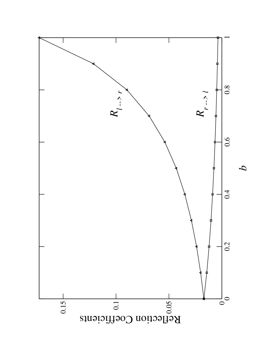
Figure 2: Coefficients $R_{l\rightarrow r}$ and $R_{r\rightarrow l}$, in the case of a smooth variation of $m(z)$, as a function of the magnetic field parameter $b$ for an energy parameter $\epsilon=7.03$, $y_{R}=4/3$, $y_{L}=1/3$. The value for the $U(1)_{Y}$ coupling constant is taken as $g^{\prime}=0.344$, corresponding to the EWPT epoch. The dots represent the computed values.

This asymmetry, built on either side of the wall, is dissociated from non-conserving baryon number processes and can subsequently be converted to baryon number in the symmetric phase where sphaleron induced transitions are taking place with a large rate. This mechanism receives the name of non-local baryogenesis CKN ; Nelson ; Dine ; Joyce and, in the absence of the external field, it can only be realized in extensions of the SM where a source of CP violation is introduced ad hoc into a complex, space-dependent phase of the Higgs field during the development of the EWPT Torrente .

In our case, the relation of this axial asymmetry to CP violation is understood as follows: recall that for instance, in the SM, CP is violated in the quark sector through the mixing between different weak interaction eigenstates to form states with definite mass. However, in the present scenario, no such mixing occurs since we are concerned only with the evolution of a single quark (e.g., the top quark) species. The relation is thus to be found in the dynamics of the scattering process itself and becomes clear once we notice that this can be thought of as describing the mixing of two levels, right- and left-handed quarks coupled to an external hypermagnetic field. When the two chirality modes interact only with the external field, they evolve separately. It is only the scattering with the bubble wall what allows a finite transition probability for one mode to become the other. Since the modes are coupled differently to the external field, these probabilities are different and give rise to the axial asymmetry. CP is violated in the process because, though C is conserved, P is violated and thus is CP.

6 Summary and outlook

In this work we have given a quantitative outline of the CP violating scattering of fermions off (a simplified picture of) EWPT bubbles in the presence of hypermagnetic fields. This scattering produces an axial asymmetry built on either side of the bubble walls. The origin of this asymmetry is the chiral nature of the fermion coupling to the hypermagnetic field in the symmetric phase. We have shown how to compute reflection and transmission coefficients and also that these differ for left and right-handed incident particles.

Primordial hypermagnetic fields thus provide with a much needed ingredient, namely, additional CP violation, for the possible generation of baryon number during the EWPT. A second ingredient, the strengthening of the order of the phase transition and thus the avoidance of the sphaleron bound seems at the moment a difficult problem to surmount. Nonetheless, it is important to bear in mind that so far, the calculations that provide insight into the effect of the hypermagnetic fields on the order of the EWPT do not account for the non-perturbative effects, cast in the language of resummation, which are otherwise well known to play a very important role for the dynamics of the phase transition in the absence of magnetic fields. Much work is needed in this direction. This is for the future.

References

- (1) A. D. Sakharov, Pis’ma Zh. Eksp. Teor. Fiz. 5, 32 (1967) [JETP Lett. 5, 24 (1967)].
- (2) M.B. Gavela, P. Hernández, J. Orloff, and O. Pène, Mod. Phys. Lett. A 9, 795 (1994).
- (3) K. Kajantie, M. Laine, K. Rummukainen, and M. Shaposnikov, Nucl. Phys. B 466, 189 (1996).
- (4) A. G. Cohen, D. B. Kaplan and A. E. Nelson, Phys. Lett. B 263, 86 (1991).
- (5) M. Carena, M. Quiros and C. E. Wagner, Nucl. Phys. B 524, 3 (1998).
- (6) J. M. Cline, Electroweak phase transition and baryogenesis, hep-ph/0201286.
- (7) M. Giovannini and M. E. Shaposhnikov, Phys. Rev. D 57, 2186 (1998).
- (8) P. Elmfors, K. Enqvist and K. Kainulainen, Phys. Lett. B 440, 269 (1998).
- (9) M. Giovannini, Primordial Magnetic Fields, hep-ph/0208152.
- (10) D. Comelli, D. Grasso, M. Pietroni and A. Riotto, Phys. Lett. B 458, 304 (1999).
- (11) M. E. Carrington, Phys. Rev. D 45, 2933 (1992).
- (12) A. Ayala, J. Besprosvany, G. Pallares and G. Piccinelli, Phys. Rev. D 64, 123529 (2001).
- (13) A. Ayala, G. Piccinelli and G. Pallares, Phys. Rev. D 66, 103503 (2002).
- (14) A. Ayala and J. Besprosvany, Nucl. Phys. B 651, 211 (2003).
- (15) A. E. Nelson, D. B. Kaplan and A. G. Cohen, Nucl. Phys. B 373, 453 (1992).
- (16) M. Trodden, Rev. Mod. Phys. 71, 1463 (1999).
- (17) A. Riotto and M. Trodden, Ann. Rev. Nucl. Part. Sci. 49, 35 (1999).
- (18) V. A. Rubakov and M. E. Shaposhnivov, Usp.Fiz.Nauk 166, 493 (1996), hep-ph/9603208.
- (19) E. W. Kolb and M. S. Turner: The Early Universe, (Addison–Wesley Publishing Company 1990).
- (20) F. W. Stecker: The matter-antimatter asymmetry of the universe. To be published in: XIVth Rencontres de Blois 2002 on Matter-Antimatter Asymmetry, ed. by J. Tran Thanh Van, hep-ph/0207323.
- (21) A. D. Dolgov: Cosmological matter-antimatter asymmetry and antimatter in the universe. To be published in: XIVth Rencontres de Blois 2002 on Matter-Antimatter Asymmetry, ed. by J. Tran Thanh Van, hep-ph/0211260.
- (22) F. R. Klinkhamer and N. S. Manton, Phys. Rev. D 30, 2212 (1984).
- (23) G. ’t Hooft, Phys. Rev. Lett. 37, 8 (1976); Phys. Rev. D 14, 3432 (1976).
- (24) For a recent review on the subject, see e.g. W. Bernreuther, Lect. Notes Phys. 591, 237 (2002), hep-ph/0205279.
- (25) V. A. Kuzmin, V. A. Rubakov and M. E. Shaposhnikov, Phys. Lett. B 155, 36 (1985).
- (26) M. E. Shaposhnikov, Nucl. Phys. B 287, 757 (1987).
- (27) K. Hagiwara et al., Phys. Rev. D 66, 010001 (2002), http://pdg.lbl.gov/.
- (28) M. Le Bellac: Thermal Field Theory, (Cambridge University Press, Cambridge 1996) pp 124–127.
- (29) K. Kajantie, M. Laine, J. Peisa, K. Rummukainen, and M. Shaposnikov, Nucl. Phys. B 544, 357 (1999).
- (30) V. Skalozub and V. Demchik, Can baryogenesis survive in the standard model due to strong hypermagnetic field?, hep-ph/9909550.
- (31) The observational situation is discussed in P.P. Kronberg, Rep. Prog. Phys. 57, 325 (1994); or more recently in J.-L. Han and R. Wielebinski, Milestones in the Observations of Cosmic Magnetic Fields, astro-ph/0209090.
- (32) R. Beck, A. Brandenburg, D. Moss, A. Shukurov and D. Sokoloff, Annu. Rev. Astron. Astrophys. 34, 155 (1996).
- (33) J. A. Eilek and F. N. Owen, Ap. J. 567, 202 (2002).
- (34) T. E. Clarke, P. P. Kronberg and H. Böhringer, Ap. J. 547, L111 (2001).
- (35) For reviews on the origin, evolution and some cosmological consequences of primordial magnetic fields see: K. Enqvist, Int. J. Mod. Phys. D7, 331 (1998); R. Maartens: Cosmological magnetic fields. In: International Conference on Gravitation and Cosmology, Pramana 55, 575 (2000) and references therein; D. Grasso and H.R. Rubinstein, Phys. Rep. 348, 163 (2001).
- (36) For quark-hadron PT: J. Quashnock, A. Loeb and D.N. Spergel, Ap. J. 344, L49 (1989); B. Cheng and A.V. Olinto, Phys. Rev. D 50, 2421 (1994); G. Sigl, A.V. Olinto and K. Jedamzik, Phys. Rev. D 55, 4582 (1997).
- (37) For EWPT: G. Baym, D. Bödeker and L. McLerran, Phys. Rev. D 53, 662 (1996).
- (38) For a PT at a critical temperature larger than EW scale: D. Boyanovsky, H. J. de Vega and M. Simionato, Large scale magnetogenesis from a non-equilibrium phase transition in the radiation dominated era, hep-ph/0211022.
- (39) T. Vachaspati, Phys. Lett. B 265, 258 (1991); T. W. B. Kibble and A. Vilenkin, Phys. Rev. D 52, 679 (1995); E.J. Copeland, P. M. Saffin and O. Törnqvist, Phys. Rev. D 61, 105005 (2000).
- (40) For an overview of the subject, see e.g., A. D. Dolgov, Generation of magnetic fields in cosmology, hep-ph/0110293.
- (41) M. S. Turner and L. M. Widrow, Phys. Rev. D 37, 2743 (1988).
- (42) B. Ratra, Ap. J. 391, L1 (1992); M. Gasperini, M. Giovannini and G. Veneziano, Phys. Rev. Lett. 75, 3796 (1995); D. Lemoine and M. Lemoine, Phys. Rev. D 52, 1955 (1995).
- (43) T. Prokopec, Cosmological magnetic fields from photon coupling to fermions and bosons in inflation, astro-ph/0106247.
- (44) J.D. Barrow, P. Ferreira and J. Silk, Phys. Rev. Lett. 78, 3610 (1997).
- (45) K. Jedamzik, V. Katalinić and A. V. Olinto, Phys. Rev. Lett. 85, 700 (2000).
- (46) J. Adams, U. H. Danielsson, D. Grasso and H. rubinstein, Phys. Lett. B 388, 253 (1996).
- (47) For the effect of stochastic magnetic fields, see A. Mack, T. Kahniashvili and A. Kosowsky, Phys.Rev. D 65, 123004 (2002), and references therein.
- (48) D. D. Harari, J. D. Hayward and M. Zaldarriaga, Phys. Rev. D 55, 1841 (1997); M Giovannini, Phys. Rev. D 56, 3198 (1997).
- (49) A. Kosowsky and A. Loeb, Ap. J. 469, 1 (1996); E. S. Scannapieco and P.G. Ferreira, Phys. Rev. D 56, 7493 (1997).
- (50) A. Ayala, J. Jalilian-Marian, L. McLerran and A. P. Vischer, Phys. Rev. D 49, 5559 (1994).
- (51) M. Dine, O. Lechtenfield, B. Sakita, W. Fischel and J. Polchinski, Nucl. Phys. B 342, 381 (1990).
- (52) M. Joyce, T. Prokopec and N. Turok, Phys. Lett. B 338, 269 (1994).
- (53) E. Torrente-Lujan, Phys. Rev. D 60, 085003 (1999).