Branching ratio and CP asymmetry of $B_{s}\to\pi^{+}\pi^{-}$
decays in the perturbative QCD approach

Abstract

In this paper, we calculate the decay rate and CP asymmetry of the $B_{s}\to\pi^{+}\pi^{-}$ decay in perturbative QCD approach with Sudakov resummation. Since none of the quarks in final states is the same as those of the initial $B_{s}$ meson, this decay can occur only via annihilation diagrams in the standard model. Besides the current-current operators, the contributions from the QCD and electroweak penguin operators are also taken into account. We find that (a) the branching ratio is about $4\times 10^{-7}$; (b) the penguin diagrams dominate the total contribution; and (c) the direct CP asymmetry is small in size: no more than $3\%$; but the mixing-induced CP asymmetry can be as large as ten percent testable in the near future LHC-b experiments.

I Introduction

In recent years, rare $B$ decays are attracting more and more attentions, since they provide a good opportunity for testing the Standard Model(SM), probing $CP$ violation and searching for possible new physics beyond the SM. Since 1999, the data sample of the pair production and decays of $B$ mesons collected by BaBar and Belle Collaborations is increased rapidly. In the future LHC-b experiments, $B_{s}$ and $B_{C}$ mesons can also be produced, and the rare $B$ decays with a branching ratio around $10^{-7}$ can be observed. The rapid progress in current $B$ factory experiments and the bright expectation in LHC-b experiments induced a great interest in the studies of rare decays of $B$ meson.

The rare decay $B_{s}\rightarrow\pi^{+}\pi^{-}$ can occur only via annihilation diagrams in SM because none of quarks in final states is the same as those of the initial $B_{s}$ meson. The usual method to treat non-leptonic decays of B meson is Factorization Approach(FA) 1 , which has achieved great success in explaining many decay branching ratios 2 ; 3 ; 4 . However, this method failed in describing $B_{s}\rightarrow\pi^{+}\pi^{-}$ decay, because we need the $\pi\rightarrow\pi$ form factor at very large momentum transfer ${\cal O}(M_{B})$. So far, little is known about the form factor at such a large momentum transfer in FA. In the QCD factorization approach 5 , one cannot perform a real calculation of the annihilation diagrams, but estimating the annihilation amplitude by introducing a phenomenological parameter. In this paper, we calculate the branching ratio and $CP$ asymmetries of $B_{s}\rightarrow\pi^{+}\pi^{-}$ decay by employing the perturbative QCD approach(PQCD) 6 . This method has been developed for the studies of the B meson decays 7 and successfully applied to calculate the annihilation diagrams 8 ; 9 . When the final states are light mesons such as pions, the perturbative QCD approach(PQCD) can be safely used because of asymptotic freedom of QCD 10 .

In the next section, we give our theoretical formulas for the decay $B_{s}\rightarrow\pi^{+}\pi^{-}$ in PQCD framework. In section 3, we give the numerical results of the branching ratio of $B_{s}\rightarrow\pi^{+}\pi^{-}$ and discuss CP asymmetry of the decay.

II Perturbative calculations

The related effective Hamiltonian for the process $B_{s}\rightarrow\pi^{+}\pi^{-}$ is given by 9 ; 11

$$H_{\mathrm{eff}}=\frac{G_{F}}{\sqrt{2}}\{V_{ub}^{*}V_{us}\left[C_{1}(\mu)O_{1}(\mu)+C_{2}(\mu)O_{2}(\mu)\right]-V_{tb}^{*}V_{ts}\sum_{i=3}^{10}C_{i}(\mu)O_{i}(\mu)\},$$ (1)

where $C_{i}(\mu)(i=1,\cdots,10)$ are Wilson coefficients at the renormalization scale $\mu$ and the operators $O_{i}(i=1,\cdots,10)$ are

$$O_{1}=(\bar{s}_{i}u_{j})_{V-A}(\bar{u}_{j}b_{i})_{V-A},\hskip 17.07164pt$$

$$O_{2}=(\bar{s}_{i}u_{i})_{V-A}(\bar{u}_{j}b_{j})_{V-A},\hskip 17.07164pt$$

$$O_{3}=(\bar{s}_{i}b_{i})_{V-A}\sum_{q}(\bar{q}_{j}q_{j})_{V-A},$$

$$O_{4}=(\bar{s}_{i}b_{j})_{V-A}\sum_{q}(\bar{q}_{j}q_{i})_{V-A},$$

$$O_{5}=(\bar{s}_{i}b_{i})_{V-A}\sum_{q}(\bar{q}_{j}q_{j})_{V+A},$$

$$O_{6}=(\bar{s}_{i}b_{j})_{V-A}\sum_{q}(\bar{q}_{j}q_{i})_{V+A},$$

$$\hskip 17.07164ptO_{7}=\frac{3}{2}(\bar{s}_{i}b_{i})_{V-A}\sum_{q}e_{q}(\bar{q}_{j}q_{j})_{V+A},$$

$$\hskip 17.07164ptO_{8}=\frac{3}{2}(\bar{s}_{i}b_{j})_{V-A}\sum_{q}e_{q}(\bar{q}_{j}q_{i})_{V+A},$$

$$\hskip 17.07164ptO_{9}=\frac{3}{2}(\bar{s}_{i}b_{i})_{V-A}\sum_{q}e_{q}(\bar{q}_{j}q_{j})_{V-A},$$

$$\hskip 17.07164ptO_{10}=\frac{3}{2}(\bar{s}_{i}b_{j})_{V-A}\sum_{q}e_{q}(\bar{q}_{j}q_{i})_{V-A}.$$ (2)

Here $i$ and $j$ are $SU(3)$ color indices, the sum over $q$ runs over the quark field that are active at the scale $\mu=O(m_{b})$, i.e., $q\in\{u,d,s,c,b\}$. Operators $O_{1},O_{2}$ come from tree level, $O_{3},O_{4},O_{5},O_{6}$ are QCD-Penguins operators and $O_{7},O_{8},O_{9},O_{10}$ come from electroweak-Penguins.

In the PQCD approach, the decay amplitude is separated into soft($\Phi$), hard($H$), and harder($C$) dynamics characterized by different scales. It is conceptually written as the following,

$$\mbox{Amplitude}\sim\int\!\!d^{4}k_{1}d^{4}k_{2}d^{4}k_{3}\ \mathrm{Tr}\bigl{[}C(t)\Phi_{B}(k_{1})\Phi_{\pi}(k_{2})\Phi_{\pi}(k_{3})H(k_{1},k_{2},k_{3},t)\bigr{]},$$ (3)

where $k_{i}$’s are momenta of light quarks included in each mesons, and $\mathrm{Tr}$ denotes the trace over Dirac and color indices. $C(t)$ is Wilson coefficient which results from the radiative corrections at short distance. $\Phi_{M}$ is wave function which describes the hadronization of mesons. The wave functions should be universal and channel independent, we can use $\Phi_{M}$ which is determined by other ways. The hard part $H$ is rather process-dependent. In the following, we start to compute the decay amplitude of $B_{s}\rightarrow\pi^{+}\pi^{-}$.

Since we set $B_{s}$ at rest, in the light-cone coordinates, the momentum of the $B_{s}$, $\pi^{-}$ and $\pi^{+}$ are written as :

$$P_{1}=\frac{M_{B}}{\sqrt{2}}(1,1,{\bf 0}_{T}),P_{2}=\frac{M_{B}}{\sqrt{2}}(1,0,{\bf 0}_{T}),P_{3}=\frac{M_{B}}{\sqrt{2}}(0,1,{\bf 0}_{T}).$$ (4)

Denoting the light (anti-)quark momenta in $B$, $\pi^{-}$ and $\pi^{+}$ as $k_{1}$, $k_{2}$ and $k_{3}$, respectively, we can choose:

$$k_{1}=(x_{1}p_{1}^{+},0,{\bf k}_{1T}),~{}~{}~{}k_{2}=(x_{2}p_{2}^{+},0,{\bf k}_{2T}),~{}~{}~{}k_{3}=(0,x_{3}p_{3}^{-},{\bf k}_{3T}).$$ (5)

According to effective Hamiltonian(1), we draw the lowest order diagrams of $B_{s}\rightarrow\pi^{+}\pi^{-}$ in Fig.1. For the factorizable diagrams (a) and (b), we find their contributions cancel each other, which is a result of exact isospin symmetry. For the non-factorizable diagrams (c) and (d), the contribution comes from tree operator is

$$M_{a}^{T}=\frac{1}{\sqrt{2N_{c}}}64\pi C_{F}M_{B}^{2}\int_{0}^{1}\!\!\!dx_{1}dx_{2}dx_{3}\int_{0}^{\infty}\!\!\!\!\!b_{1}db_{1}\,b_{2}db_{2}\ \phi_{B}(x_{1},b_{1})\\ \times\Bigl{[}C_{2}(t_{1})\alpha_{s}(t_{1})\bigl{\{}-x_{3}\phi_{\pi}^{A}(x_{2})\phi_{\pi}^{A}(x_{3})-r^{2}(x_{2}+x_{3})\phi_{\pi}^{P}(x_{2})\phi_{\pi}^{P}(x_{3})\\ +r^{2}(x_{2}-x_{3})\phi_{\pi}^{P}(x_{2})\phi_{\pi}^{T}(x_{3})+r^{2}(x_{2}-x_{3})\phi_{\pi}^{P}(x_{3})\phi_{\pi}^{T}(x_{2})\\ -r^{2}(x_{2}+x_{3})\phi_{\pi}^{T}(x_{2})\phi_{\pi}^{T}(x_{3})\bigr{\}}h_{a}^{(1)}(x_{1},x_{2},x_{3},b_{1},b_{2})E_{m}(t_{1})\\ +C_{2}(t_{2})\alpha_{s}(t_{2})\bigl{\{}x_{2}\phi_{\pi}^{A}(x_{2})\phi_{\pi}^{A}(x_{3})+r^{2}(2+x_{2}+x_{3})\phi_{\pi}^{P}(x_{2})\phi_{\pi}^{P}(x_{3})\\ +r^{2}(x_{2}-x_{3})\phi_{\pi}^{P}(x_{2})\phi_{\pi}^{T}(x_{3})+r^{2}(x_{2}-x_{3})\phi_{\pi}^{T}(x_{2})\phi_{\pi}^{P}(x_{3})\\ +r^{2}(-2+x_{2}+x_{3})\phi_{\pi}^{T}(x_{2})\phi_{\pi}^{T}(x_{3})\bigr{\}}h_{a}^{(2)}(x_{1},x_{2},x_{3},b_{1},b_{2})E_{m}(t_{2})\bigr{]},$$ (6)

where $r=m_{0\pi}/m_{B}=m_{\pi}^{2}/[m_{B}(m_{u}+m_{d})]$. $C_{F}=4/3$ is the group factor of the $SU(3)_{c}$ gauge group. The expressions of the meson distribution amplitudes $\phi_{M}$, the Sudakov factor $E_{m}(t_{i})$ and the functions $h_{a}^{(1,2)}(x_{1},x_{2},x_{3},b_{1},b_{2})$ are given in the appendix. The contribution of penguin-diagrams $M_{a}^{P}$ can be obtained by replacing $C_{2}(t_{i})(i=1,2)$ with

$$a^{P}(t_{i})=2C_{4}(t_{i})+2C_{6}(t_{i})+\frac{1}{2}C_{8}(t_{i})+\frac{1}{2}C_{10}(t_{i}),$$ (7)

in Eq.(6). The explicit expressions of QCD corrected Wilson coefficients $C_{2}$, $C_{4}$, $C_{6}$, $C_{8}$ and $C_{10}$ as a function of scale $t$ can be found in the Appendix of Ref.9 .

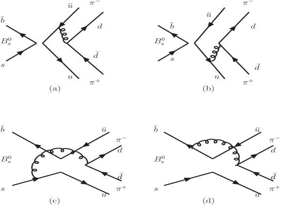
Figure 1: The lowest order diagrams for $B_{s}^{0}\to\pi^{+}\pi^{-}$ decay.

Now, the total decay amplitude for $B_{s}\rightarrow\pi^{+}\pi^{-}$ is given by

$$A=V_{ub}^{*}V_{us}M_{a}^{T}-V_{tb}^{*}V_{ts}M_{a}^{P}=V_{ub}^{*}V_{us}M_{a}^{T}[1+ze^{i(\delta-\gamma)}],$$ (8)

where $z=|V_{tb}^{*}V_{ts}/V_{ub}^{*}V_{us}||M_{a}^{P}/M_{a}^{T}|$, $V_{ub}\simeq|V_{ub}|e^{-i\gamma}$ and $\delta$ is the relative strong phase between tree diagrams($M_{a}^{T}$) and penguin diagrams($M_{a}^{P}$). z and $\delta$ can be calculated from PQCD.

The decay width is expressed as

$$\Gamma(B_{s}^{0}\to\pi^{+}\pi^{-})=\frac{G_{F}^{2}M_{B}^{3}}{128\pi}|A|^{2}=\frac{G_{F}^{2}M_{B}^{3}}{128\pi}|V_{ub}^{*}V_{us}M_{a}^{T}|^{2}[1+z^{2}+2z\cos(\delta-\gamma)].$$ (9)

Similarly, we can get the decay width for $\bar{B}^{0}_{s}\rightarrow\pi^{+}\pi^{-}$

$$\Gamma(\bar{B}_{s}^{0}\to\pi^{+}\pi^{-})=\frac{G_{F}^{2}M_{B}^{3}}{128\pi}|\bar{A}|^{2},$$ (10)

where

$$\bar{A}=V_{ub}V_{us}^{*}M_{a}^{T}-V_{tb}V_{ts}^{*}M_{a}^{P}=V_{ub}V_{us}^{*}M_{a}^{T}[1+ze^{i(\delta+\gamma)}].$$ (11)

III Numerical evaluation and summary

The following parameters have been used in our numerical calculation:

$$M_{B_{s}}=5.37\mbox{ GeV},\ m_{0\pi}=1.4\mbox{ GeV},\ \Lambda^{f=4}_{QCD}=0.25\mbox{ GeV},f_{B_{s}}=236\mbox{ MeV},\$$

$$f_{\pi}=130\mbox{ MeV},\ \tau_{B_{s}^{0}}=1.46\times 10^{-12}\mbox{s},|V_{tb}^{*}V_{ts}|=0.0395,|V_{ub}^{*}V_{us}|=0.0008.$$ (12)

We leave the CKM phase angle $\gamma$ as a free parameter to explore the branching ratio and CP asymmetry parameter dependence on it. In SM, the CKM phase angle is the origin of CP violation.

From Eq.(9) and (10), we get the averaged decay width for $B_{s}^{0}(\bar{B}^{0}_{s})\rightarrow\pi^{+}\pi^{-}$

$$\Gamma(B_{s}^{0}(\bar{B}^{0}_{s})\to\pi^{+}\pi^{-}) = \frac{G_{F}^{2}M_{B}^{3}}{128\pi}(|A|^{2}/2+|\bar{A}|^{2}/2)\hskip 28.45274pt$$ (13)

$$= \frac{G_{F}^{2}M_{B}^{3}}{128\pi}|V_{ub}^{*}V_{us}M_{a}^{T}|^{2}[1+2z\cos\gamma\cos\delta+z^{2}].$$

Using the above parameters, we get $z=13.4$ and $\delta=168^{\circ}$ in PQCD. Eq.(13) is a function of CKM angle $\gamma$. In Fig. 2, we plot the averaged branching ratio of the decay $B_{s}^{0}(\bar{B}^{0}_{s})\rightarrow\pi^{+}\pi^{-}$ with respect to the parameter $\gamma$. From Fig. 2, we can see that :

$$\mathbf{Br}(B_{s}^{0}(\bar{B}^{0}_{s})\to\pi^{+}\pi^{-})=(4.2\pm 0.6)\times 10^{-7},$$ (14)

for $0<\gamma<\pi$. The number $z=|V_{tb}^{*}V_{ts}/V_{ub}^{*}V_{us}||M_{a}^{P}/M_{a}^{T}|=13.4$ means the amplitude of penguin diagrams is about 13.4 times more than that of tree diagrams. Therefore almost all the contribution comes from penguin diagrams in this decay and the branching ratio is not sensitive to $\gamma$.

In Ref.17 , Beneke et al have estimated the branching ratio for $B_{s}\to\pi^{+}\pi^{-}$ in QCD Factorization approach. In order to avoid the endpoint singularities, they introduced parameters to replace the divergent integral. In this approach, they estimated that the branching ratio of this decay is $(0.24-1.55)\times 10^{-7}$ with those phenomenological parameters. In our work, the calculation has no endpoint singularity because of $k_{T}$6 . Our predicted result is larger than their simple estimation, which can be tested by the experiments.

For the experimental side, we notice that there is only upper limit of the decay $B_{s}^{0}\to\pi^{+}\pi^{-}$ given at $90\%$ confidence level 12

$$\mathrm{Br}(B_{s}^{0}\to\pi^{+}\pi^{-})<1.4\times 10^{-4}.$$ (15)

Obviously, our predicted result is still far from this upper limit.

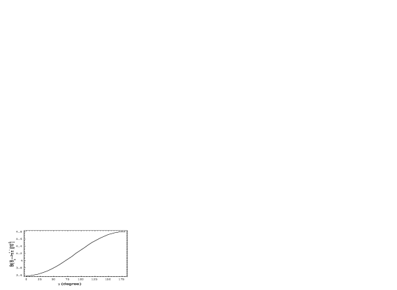
Figure 2: The CP-averaged branching ratio of $B_{s}^{0}(\bar{B}_{s})\to\pi^{+}\pi^{-}$ decay as a function of CKM angle $\gamma$.

In SM, CP violation comes from interference between amplitudes with different CP eigenvalues. The strong interaction eigenstates $B_{s}^{0}$ and $\bar{B}_{s}^{0}$ can mix through weak interaction, i.e. $B_{s}^{0}$-$\bar{B}_{s}^{0}$ oscillation. By experimental observation we can know whether CP is conserved. For the $B_{s}^{0}$-$\bar{B}_{s}^{0}$ system, the CP asymmetry is time dependent 3 ; 13 :

$$A_{CP}(t)\simeq A_{CP}^{dir}\cos(\Delta mt)+a_{\epsilon+\epsilon^{{}^{\prime}}}\sin(\Delta mt),$$ (16)

where $\Delta m$ is the mass difference of the two mass eigenstates of $B_{s}$ mesons. $A_{CP}^{dir}$ is the direct CP violation parameter while $a_{\epsilon+\epsilon^{{}^{\prime}}}$ is the mixing-related CP violation parameter. The direct CP violation parameter is defined as

$$A_{CP}^{dir}=\frac{\Gamma(B_{s}^{0}\rightarrow\pi^{+}\pi^{-})-\Gamma(\bar{B}_{s}^{0}\rightarrow\pi^{+}\pi^{-})}{\Gamma(B_{s}^{0}\rightarrow\pi^{+}\pi^{-})+\Gamma(\bar{B}_{s}^{0}\rightarrow\pi^{+}\pi^{-})}=\frac{2z\sin\gamma\sin\delta}{1+2z\cos\gamma\cos\delta+z^{2}}.$$ (17)

Using Eq.(9) and (10), we can compute the parameter $A_{CP}^{dir}$. The direct CP asymmetry $A_{CP}^{dir}$ has a strong dependence on the CKM angle, as can be seen easily from Eq.(17) and Fig. 3. From this figure one can see that when the CKM angle $\gamma$ is around $\pi/2$ the direct CP asymmetry reaches its peak, which is about $3\%$. The small direct CP asymmetry is also a result of small tree level contribution.

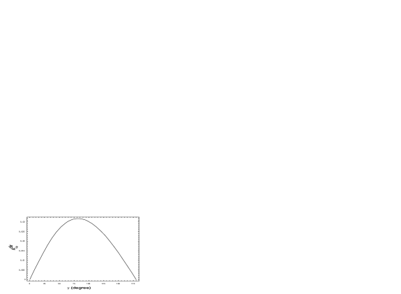
Figure 3: Direct CP violation parameters of $B_{s}\to\pi^{+}\pi^{-}$ decay as a function of CKM angle $\gamma$.

The mixing-related CP violation parameter in Eq.(16) is defined as 9

$$a_{\epsilon+\epsilon^{{}^{\prime}}}=\frac{-2Im(\lambda_{CP})}{1+|\lambda_{CP}|^{2}},$$ (18)

where

$$\lambda_{CP}=\frac{V_{tb}^{*}V_{ts}\langle f|H_{eff}|\bar{B}_{s}^{0}\rangle}{V_{tb}V_{ts}^{*}\langle f|H_{eff}|B_{s}^{0}\rangle}.$$ (19)

In Fig. 4, we study the mixing CP violation parameter $a_{\epsilon+\epsilon^{{}^{\prime}}}$ of the decay $B_{s}\rightarrow\pi^{+}\pi^{-}$ as a function of CKM angle $\gamma$, just like the case of direct CP violation, it is almost symmetric and the symmetry axis is near $\gamma=\pi/2$. its peak is close to $-14.5\%$. The possible large CP asymmetry might be observed at LHCb experiment in the future, this would help us to determine the value of CKM angle $\gamma$.

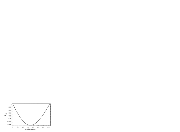
Figure 4: Mixing-related CP violation parameter $a_{\epsilon+\epsilon^{{}^{\prime}}}$ of $B_{s}^{0}(\bar{B}_{s})\to\pi^{+}\pi^{-}$ decay as a function of CKM angle $\gamma$.

In conclusion, we study the branching ratio and CP asymmetry of the decay $B_{s}^{0}(\bar{B}^{0}_{s})\rightarrow\pi^{+}\pi^{-}$ in PQCD, we find that the branching ratio is at the order of $10^{-7}$ and there are large CP asymmetries in the process, which may be measured in the future LHC-b experiments and BTeV experiment at Fermilab. This small branching ratio, predicted in the SM, make it sensitive to possible new physics contribution.

Appendix A Some formulas used in the text

For $B_{s}$ meson wave function, we use the same wave function as $B$ meson 9 ; 14 , despite the possible SU(3) breaking effect

$$\phi_{B_{s}}(x,b)=N_{B_{s}}x^{2}(1-x)^{2}\exp\left[-\frac{M_{B_{s}}^{2}\ x^{2}}{2\omega_{b}^{2}}-\frac{1}{2}(\omega_{b}b)^{2}\right].$$ (20)

The parameter $\omega_{b}=0.4\mbox{ GeV}$, is constrained by other charmless B decays 9 ; 14 . And $N_{B_{s}}=114.0\mbox{GeV}$ is the normalization constant using $f_{B_{s}}=236\mbox{MeV}$.

The $\pi$ meson’s distribution amplitudes are given by light cone QCD sum rules 15 :

$$\phi_{\pi}^{A}(x) = \frac{3f_{\pi}}{\sqrt{2N_{c}}}x(1-x)\left\{1+0.44C_{2}^{3/2}(t)+0.25C_{4}^{3/2}(t)\right\},$$

$$\phi_{\pi}^{P}(x) = \frac{f_{\pi}}{2\sqrt{2N_{c}}}\left\{1+0.43C_{2}^{1/2}(t)+0.09C_{4}^{1/2}(t)\right\},$$

$$\phi_{\pi}^{T}(x) = \frac{f_{\pi}}{2\sqrt{2N_{c}}}(1-2x)\left\{1+0.55(10x^{2}-10x+1)\right\},$$ (21)

where $t=1-2x$. The Gegenbauer polynomials are defined by:

$$C_{2}^{1/2}(t)=\frac{1}{2}(3t^{2}-1),\hskip 28.45274ptC_{4}^{1/2}(t)=\frac{1}{8}(35t^{4}-30t^{2}+3),$$

$$C_{2}^{3/2}(t)=\frac{3}{2}(5t^{2}-1),\hskip 28.45274ptC_{4}^{3/2}(t)=\frac{15}{8}(21t^{4}-14t^{2}+1).$$ (22)

Since the hard part is calculated only to leading order of $\alpha_{s}$, we use the one loop expression for the strong running coupling constant in our numerical analysis,

$$\alpha_{s}(\mu)=\frac{4\pi}{\beta_{0}\mathrm{ln}(\mu^{2}/\Lambda^{2})},$$ (23)

where $\beta_{0}=(33-2n_{f})/3$ and $n_{f}$ is the number of active quark flavor at the appropriate scale $\mu$. $\Lambda$ is the QCD scale, we set $\Lambda=250$MeV at $n_{f}=4$.

The function $E_{m}(t_{i})$ in Eq.(6) are defined by

$$E_{m}(t_{i})=e^{-S_{B}(t_{i})-S_{\pi^{+}}(t_{i})-S_{\pi^{-}}(t_{i})},$$ (24)

where $S_{B}$, $S_{\pi^{+}}$, $S_{\pi^{-}}$ result from summing both double logarithms due to infrared gluon corrections and single ones caused by the renormalization of ultra-violet divergence. They are defined as:

$$S_{B}(t)=s(x_{1}P_{1}^{+},b_{1})+2\int_{1/b_{1}}^{t}\!\!\!\frac{d\bar{\mu}}{\bar{\mu}}\gamma(\alpha_{s}(\bar{\mu})),\hskip 99.58464pt$$ (25)

$$S_{\pi^{-}}(t)=s(x_{2}P_{2}^{+},b_{2})+s((1-x_{2})P_{2}^{+},b_{2})+2\int_{1/b_{2}}^{t}\!\!\!\frac{d\bar{\mu}}{\bar{\mu}}\gamma(\alpha_{s}(\bar{\mu}))$$ (26)

$$S_{\pi^{+}}(t)=s(x_{3}P_{3}^{-},b_{3})+s((1-x_{3})P_{3}^{-},b_{3})+2\int_{1/b_{3}}^{t}\!\!\!\frac{d\bar{\mu}}{\bar{\mu}}\gamma(\alpha_{s}(\bar{\mu})),$$ (27)

where $s(Q,b)$ called Sudakov factor is given as 16

$$s(Q,b)=\int_{1/b}^{Q}\!\!\!\frac{d\mu}{\mu}\Bigl{[}\ln\left(\frac{Q}{\mu}\right)A(\alpha(\bar{\mu}))+B(\alpha_{s}(\bar{\mu}))\Bigr{]}$$ (28)

with

$$A=C_{F}\frac{\alpha_{s}}{\pi}+\left[\frac{67}{9}-\frac{\pi^{2}}{3}-\frac{10}{27}n_{f}+\frac{2}{3}\beta_{0}\ln\left(\frac{e^{\gamma_{E}}}{2}\right)\right]\left(\frac{\alpha_{s}}{\pi}\right)^{2},$$ (29)

$$B=\frac{2}{3}\frac{\alpha_{s}}{\pi}\ln\left(\frac{e^{2\gamma_{E}-1}}{2}\right)\hskip 170.71652pt$$ (30)

here $\gamma_{E}$ is the Euler constant, $n_{f}$ is the active flavor number.

The functions $h_{a}^{(1)}$, and $h_{a}^{(2)}$ in Eq.(6) come from the Fourier transformation of propagators of virtual quark and gluon. They are defined by

$$h^{(j)}_{a}(x_{1},x_{2},x_{3},b_{1},b_{2})=$$

$$\biggl{\{}\frac{\pi i}{2}\mathrm{H}_{0}^{(1)}(M_{B}\sqrt{x_{2}x_{3}}\,b_{1})\mathrm{J}_{0}(M_{B}\sqrt{x_{2}x_{3}}\,b_{2})\theta(b_{1}-b_{2})$$

$$\qquad\qquad\qquad\qquad+(b_{1}\leftrightarrow b_{2})\biggr{\}}\times\left(\begin{matrix}\mathrm{K}_{0}(M_{B}F_{(j)}b_{1}),&\text{for}\quad F^{2}_{(j)}>0\\ \frac{\pi i}{2}\mathrm{H}_{0}^{(1)}(M_{B}\sqrt{|F^{2}_{(j)}|}\ b_{1}),&\text{for}\quad F^{2}_{(j)}<0\end{matrix}\right),$$ (31)

where $\mathrm{H}_{0}^{(1)}(z)=\mathrm{J}_{0}(z)+i\,\mathrm{Y}_{0}(z)$, and $F_{(j)}$s are defined by

$$F^{2}_{(1)}=x_{1}x_{3}-x_{2}x_{3},\ F^{2}_{(2)}=x_{1}+x_{2}+x_{3}-x_{1}x_{3}-x_{2}x_{3}.$$ (32)

The hard scale $t_{i}(i=1,2)$ in Eq.(6) are taken as the largest energy scale in the $H$ to kill the large logarithmic radiative corrections:

$$t_{i}=\mathrm{max}(M_{B}\sqrt{|F^{2}_{(i)}|},M_{B}\sqrt{x_{2}x_{3}},1/b_{1},1/b_{2})\hskip 28.45274pt(i=1,2).$$ (33)