Sensitivity of Supersymmetric Dark Matter
to the b Quark Mass

Mario E Gómez^a,b, Tarek Ibrahim^c,d, Pran Nath^d and Solveig Skadhauge^b

a. Departamento de Física Aplicada, Facultad de Ciencias Experimentales,
Universidad de Huelva, 21071 Huelva, Spain
b. Departamento de Física, Instituto Superior Técnico, Av. Rovisco Pais, 1049-001 Lisboa, Portugal.
c. Department of Physics, Faculty of Science, University of Alexandria,
Alexandria, Egypt
d. Department of Physics, Northeastern University, Boston, MA 02115-5000, USA.

Abstract

An analysis of the sensitivity of supersymmetric dark matter to variations in the b quark mass is given. Specifically we study the effects on the neutralino relic abundance from supersymmetric loop corrections to the mass of the b quark. It is known that these loop corrections can become significant for large $\tan\beta$. The analysis is carried out in the framework of mSUGRA and we focus on the region where the relic density constraints are satisfied by resonant annihilation through the s-channel Higgs poles. We extend the analysis to include CP phases taking into account the mixing of the CP-even and CP-odd Higgs boson states which play an important role in determining the relic density. Implications of the analysis for the neutralino relic density consistent with the recent WMAP relic density constraints are discussed.

1 Introduction

There is now a convincing body of evidence that the universe has a considerable amount of non baryonic dark matter and the recent Wilkinson Microwave Anisotropy Probe (WMAP) data allows a determination of cold dark matter (CDM) to lie in the range[1, 2]

$$\Omega_{CDM}h^{2}=0.1126^{+0.008}_{-0.009}$$ (1)

One expects the Milky Way to have a similar density of cold dark matter and thus there are several ongoing experiments as well as experiments that are planned for the future for its detection in the laboratory[3, 4, 5, 6, 7]. One prime CDM candidate that appears naturally in the framework of SUGRA models[8] is the neutralino[9]. We will work within the framework of SUGRA models which have a constrained parameter space. Thus without CP phases the mSUGRA parameter space is given by the parameters $m_{0},m_{\frac{1}{2}},A_{0},\tan\beta$ and $sign(\mu)$ where $m_{0}$ is the universal scalar mass, $m_{\frac{1}{2}}$ is the universal gaugino mass, $A_{0}$ is the universal trilinear coupling (all given at the grand unification scale $M_{G}$), $\tan\beta=\langle H_{2}\rangle/\langle H_{1}\rangle$ where $H_{2}$ gives mass to the up quark and $H_{1}$ gives mass to the down quark and the lepton, and $\mu$ is the Higgs mixing parameter which appears in the super potential in the form $\mu H_{1}H_{2}$. SUGRA models allow for nonuniversalities and with nonuniversalities the parameter space of the model is enlarged. Thus, for example, SUGRA models with gauge kinetic energy functions that are not singlets of the $SU(3)\times SU(2)\times U(1)$ gauge groups allow for nonuniversal gaugino masses $\tilde{m}_{i}$ (i=1,2,3) at the grand unification scale. The parameter space of SUGRA models is further enlarged when one allows for the CP phases. Thus in general $\mu$, $A_{0}$ and $\tilde{m}_{i}$ become complex allowing for phases $\theta_{\mu}$, $\alpha_{A_{0}}$, and $\xi_{i}$ where $\theta_{\mu}$ is the $\mu$ phase, $\alpha_{A_{0}}$ is the $A_{0}$ phase and $\xi_{i}$ is the phase of the gaugino mass $\tilde{m}_{i}$ ($i$=1,2,,3). Not all the phases are independent after one performs field redefinitions, and only specific combinations of them appear in physical processes[10].

In most of the mSUGRA parameter space the neutralino relic density is too large. However, there are four distinguishable regions where a neutralino relic density compatible with the WMAP constraints can be found. These regions are discussed below. (I) The bulk region: This region corresponds to relatively small values of $m_{0}$ and $m_{\frac{1}{2}}$ and is dominated by sfermion exchange diagrams. However, it is almost ruled out by the laboratory experiments. (II) The Hyperbolic Branch or Focus Point region (HB/FP)[11]: This region occurs for very high values of $m_{0}$ and small values of $\mu$ and is thus close to the domain where the electroweak symmetry breaking does not occur. Here the lightest neutralino has a large Higgsino component, thereby enhancing the annihilation cross-section to gauge boson channels. Furthermore, chargino coannihilation contributes as the chargino and the lightest neutralino are almost degenerate. (III) The stau coannihilation region: In this region $m_{\tilde{\tau}}\simeq m_{\chi}$ and the annihilation cross-section increases due to coannihilations $\chi\tilde{\tau}_{1}$. (IV) The resonant region: This is a rather broad region where the relic density constraints are satisfied by annihilation through resonant s-channel Higgs exchange. In this work we will mainly focus on, this resonant region.

While there are many analyses of the neutralino relic density there are no in depth analyses of its sensitivity to the b quark mass. One of the purposes of this analysis is to investigate this sensitivity. Such an analysis is relevant since experimentally the mass of the b quark has an error corridor, and secondly because in supersymmetric theories loop corrections to the b quark mass especially for large $\tan\beta$ can be large and model dependent[12]. Recently, a full analysis of one loop contribution to the bottom quark mass ($m_{b}$) including phases was given[13] and indeed corrections to $m_{b}$ are found to be as much as 50% or more in some regions of the parameter space. Further, $m_{b}$ corrections are found to affect considerably low energy phenomenology where the b quark enters[14, 15]. As noted above the $m_{b}$ corrections are naturally large for large $\tan\beta$ which is an interesting region because of the possibility of Yukawa unification[16, 17] and also because it leads to large neutralino-proton cross-sections[18] which makes the observation of supersymmetric dark matter more accessible. However, we do not address the issue of Yukawa unification or of neutralino-proton cross-sections in this paper. We will also discuss the dependence of the relic density on phases. It has been realized for some time that large phases can be accommodated without violating the electric dipole moment (EDM) constraints[19, 20, 21, 22] by a variety of ways which include mass suppression[23], the cancellation mechanism[24, 25], phases only in the third generation[26], and other mechanisms[27]. One of the important consequences of such phases is that the Higgs mass eigenstates are no longer eigenstates of CP[28, 29, 30, 31]. It was pointed out some time ago that CP phases would affect dark matter significantly in regions where the neutralino annihilation was dominated by the resonant Higgs annihilation[29, 32]. We discuss this issue in greater detail in this paper.

Since the focus of this paper is on the effects of loop corrections to the b quark mass, we briefly discuss these corrections. For the b quark the running mass $m_{b}(Q)$ and the physical mass, or the pole mass $M_{b}$, are related by inclusion of QCD corrections and at the two loop level one has[33]

$$M_{b}=(1+\frac{4\alpha_{3}(M_{b})}{3\pi}+12.4\frac{\alpha_{3}(M_{b})^{2}}{\pi^{2}})m_{b}(M_{b})$$ (2)

where $m_{b}(M_{b})$ is obtained from $m_{b}(M_{Z})$ by using the renormalization group equations and $m_{b}(M_{Z})$ is the running $b$ quark mass at the scale of the $Z$ boson mass defined by

$$m_{b}(M_{Z})=h_{b}(M_{Z})\frac{v}{\sqrt{2}}\cos\beta(1+\Delta m_{b})\;.$$ (3)

Here $h_{b}(M_{Z})$ is the Yukawa coupling and $\Delta m_{b}$ is loop correction to $m_{b}$. Now the coupling of the b quark to the Higgs at the tree level involves only the neutral component of the $H_{1}$ Higgs boson and the couplings to the $H_{2}$ Higgs boson is absent. However, at the loop level one finds corrections to the $H_{1}^{0}$ coupling as well as an additional coupling to $H_{2}^{0}$. Thus at the loop level the effective b quark coupling with the Higgs is given by[34]

$$-L_{bbH^{0}}=(h_{b}+\delta h_{b})\bar{b}_{R}b_{L}H_{1}^{0}+\Delta h_{b}\bar{b}_{R}b_{L}H_{2}^{0}+H.c.$$ (4)

The correction to the b quark mass is then given directly in terms of $\Delta h_{b}$ and $\delta h_{b}$ so that

$$\Delta m_{b}=[Re(\frac{\Delta h_{b}}{h_{b}})\tan\beta+Re(\frac{\delta h_{b}}{h_{b}})]$$ (5)

A full analysis of $\Delta m_{b}$ is given in Ref.[13] and we will use that analysis in this work.

Figure 1: Feynman diagrams responsible for the main contribution to the neutralino annihilation cross-section in the region of the parameter space investigated in this analysis. Fig.(a) gives the s-channel Higgs exchange contribution and Fig.(b) gives the t- and u-channel sfermion exchange contribution to the neutralino annihilation cross-section. The most important decay channels for large $\tan\beta$ are for $f=b,\tau$.

2 CP-even, CP-odd Higgs Mixing and b Quark Mass Corrections

As already mentioned we will focus on determining the sensitivity of the relic density to the b quark mass in the region with resonant s-channel Higgs dominance. This region is characterized roughly by the constraint

$$2m_{\chi}\simeq m_{A}\;.$$ (6)

The satisfaction of the relic density constraints consistent with WMAP in this case depends sensitively on the difference $\delta=(2m_{\chi}-m_{A})$ which in turn depends sensitively on the mSUGRA parameter space. In this context the bottom mass corrections are very important as the value of $m_{A}$ is strongly dependent on it, as shown in Fig.(2). On the other hand at least for the domain where the neutralino is Bino like one finds that the neutralino mass $m_{\chi}$ is rather insensitive to the bottom mass correction and is almost entirely determined by $m_{\frac{1}{2}}$.

Figure 2: The pseudo scalar Higgs boson mass $m_{A}$ as a function of $\Delta m_{b}$ for fixed values of $\tan\beta$ of 40, 50 and 60 when $m_{0}=m_{\frac{1}{2}}=A_{0}=600$ GeV.

The resonant s-channel region is only open at large $\tan\beta$. The exact allowed range of $\tan\beta$ depends severely on the value of the bottom quark mass. For $\mu<0$ the resonant region is typically open for $\tan\beta$ in the range 35-45 and for $\mu>0$ for $\tan\beta$ in the range 45-55. The large $\tan\beta$ regime is also interesting for other reasons, as in the presence of CP violation there can be a large mixing between the CP-even and the CP-odd states. Moreover, the CP phases have a strong impact on the b quark mass. In this section we discuss the relevant part of the analysis related to these effects. It is clear that if the CP phases influence the resonance condition, or equivalently the ratio $m_{\chi}/m_{A}$, they will have an impact on the relic density. This ratio is affected by phases mainly because $m_{A}$ is strongly dependent on the bottom mass correction $\Delta m_{b}$ and through it on the CP phases. Furthermore, the Higgs couplings relevant for computing the annihilation cross-section depend on the CP phases. Thus we expect the relic density to be strongly dependent on the CP phases.

We begin by considering the s-channel decay to a pair of fermions, as shown in Fig.(1)(a). The Yukawa coupling correction enters clearly here in the vertex of the neutral Higgs with the fermion pair. The amplitude for $\chi(p_{1})\chi(p_{2})\rightarrow f(k_{1})\bar{f}(k_{2})$, mediated by Higgs mass eigenstates, $H_{k},\;k=1,2,3$ may be written as,

$$M_{k}^{f}=\bar{v}(p_{2})\left[S_{k}^{\prime}-iS_{k}^{\prime\prime}\gamma_{5}\right]u(p_{1})\frac{1}{-M_{H_{k}}^{2}+s-iM_{H_{k}}\Gamma_{H_{k}}}\bar{u}(k_{1})\left[C^{S}_{f,k}+iC^{P}_{f,k}\gamma_{5}\right]v(k_{2})$$ (7)

where

$$S^{\prime}_{k}=\frac{gm_{\chi}R_{k2}}{2M_{w}\sin\beta}+Re(A_{k}),$$ (8)

$$S^{\prime\prime}_{k}=-\frac{gm_{\chi}R_{k3}\cot\beta}{2M_{w}}+Im(A_{k}).$$ (9)

and the parameters $A_{k}$ are defined by

$$A_{k}=Q^{\prime\prime*}_{00}R_{k1}-iQ^{\prime\prime*}_{00}R_{k3}\sin\beta-\frac{1}{\sin\beta}(R_{k2}-iR_{k3}\cos\beta)(Q^{\prime\prime*}_{00}\cos\beta+R^{\prime\prime*}_{00}),$$ (10)

where

$$Q^{\prime\prime}_{00}=X_{30}^{*}(X_{20}^{*}-\tan\theta_{W}X_{10}^{*})$$ (11)

and

$$R^{\prime\prime}_{00}=\frac{1}{2M_{w}}[\tilde{m}_{2}X^{*2}_{20}+\tilde{m}_{1}X^{*2}_{10}-2\mu^{*}X_{30}^{*}X_{40}^{*}].$$ (12)

Here $X$ is the matrix that diagonalizes the neutralino mass matrix so that $X^{T}M_{\chi}X$ = $diag(m_{\chi_{1}},m_{\chi_{2}},m_{\chi_{3}},m_{\chi_{4}})$ and $m_{\chi_{0}}$ is the lightest neutralino. Thus 0 is the index among $1,2,3,4$ that corresponds to the lightest neutralino (later in the analysis we will drop the subscript on $\chi_{0}$ and $\chi$ will stand for the lightest neutralino).

Since the CP effects in the Higgs sector play an important role in this analysis, we briefly review the main aspects of this phenomena. In the presence of explicit CP violation the two Higgs doublets of the supersymmetric standard model (MSSM) can be decomposed as follows

$$(H_{1})=\left(\matrix{H_{1}^{0}\cr H_{1}^{-}}\right)=\frac{1}{\sqrt{2}}\left(\matrix{v_{1}+\phi_{1}+i\psi_{1}\cr H_{1}^{-^{\prime}}}\right)$$

$$(H_{2})=\left(\matrix{H_{2}^{+}\cr H_{2}^{0}}\right)=\frac{e^{i\theta_{H}}}{\sqrt{2}}\left(\matrix{H_{2}^{+^{\prime}}\cr v_{2}+\phi_{2}+i\psi_{2}}\right)$$ (13)

where $\phi_{1},\phi_{2},\psi_{1},\psi_{2}$ are real quantum fields and $\theta_{H}$ is a phase. Variations with respect to the fields give

$$-\frac{1}{v_{1}}(\frac{\partial\Delta V}{\partial\phi_{1}})_{0}=m_{1}^{2}+\frac{g_{2}^{2}+g_{Y}^{2}}{8}(v_{1}^{2}-v_{2}^{2})+m_{3}^{2}\tan\beta\cos\theta_{H}$$

$$-\frac{1}{v_{2}}(\frac{\partial\Delta V}{\partial\phi_{2}})_{0}=m_{2}^{2}-\frac{g_{2}^{2}+g_{Y}^{2}}{8}(v_{1}^{2}-v_{2}^{2})+m_{3}^{2}\cot\beta\cos\theta_{H}$$

$$\frac{1}{v_{1}}(\frac{\partial\Delta V}{\partial\psi_{2}})_{0}=m_{3}^{2}\sin\theta_{H}=\frac{1}{v_{2}}(\frac{\partial\Delta V}{\partial\psi_{1}})_{0}$$ (14)

where $m_{1},m_{2},m_{3}$ are the parameters that enter in the tree-level Higgs potential, i.e., $V_{0}=$ $m_{1}^{2}|H_{1}|^{2}+m_{2}^{2}|H_{2}|^{2}+(m_{3}^{2}H_{1}.H_{2}+H.c.)+V_{D}$ where $V_{D}$ is the D-term contribution, $g_{2}$ and $g_{Y}$ are the gauge coupling constants for $SU(2)$ and $U(1)_{Y}$ gauge groups, and $\Delta V$ is the loop correction to the Higgs potential. In the above the subscript 0 denotes that the quantities are computed at the point where $\phi_{1}=\phi_{2}=\psi_{1}=\psi_{2}=0$. Eq.(14) provides a determination of $\theta_{H}$. Computations in the above basis lead to a $4\times 4$ Higgs mass matrix. It is useful to introduce a new basis $\{\phi_{1},\phi_{2},\psi_{1D},\psi_{2D}\}$ where $\psi_{1D},\psi_{2D}$ are defined by

$$\psi_{1D}=\sin\beta\psi_{1}+\cos\beta\psi_{2}$$

$$\psi_{2D}=-\cos\beta\psi_{1}+\sin\beta\psi_{2}$$ (15)

In the new basis the field $\psi_{2D}$ exhibits itself as the Goldstone field and decouples from the other three fields $\{\phi_{1},\phi_{2},\psi_{1D}\}$ and the Higgs mass matrix in the new basis takes on the form

$$M^{2}_{\rm Higgs}=\left(\matrix{M_{Z}^{2}c_{\beta}^{2}+m_{A}^{2}s_{\beta}^{2}+\Delta_{11}&-(M_{Z}^{2}+m_{A}^{2})s_{\beta}c_{\beta}+\Delta_{12}&\Delta_{13}\cr-(M_{Z}^{2}+m_{A}^{2})s_{\beta}c_{\beta}+\Delta_{12}&M_{Z}^{2}s_{\beta}^{2}+m_{A}^{2}c_{\beta}^{2}+\Delta_{22}&\Delta_{23}\cr\Delta_{13}&\Delta_{23}&(m_{A}^{2}+\Delta_{33})}\right)$$ (16)

where $m_{A}$ is the mass of the CP-odd Higgs boson at the tree level, $M_{Z}$ is the Z boson mass, $s_{\beta}(c_{\beta})=\sin\beta(\cos\beta)$, and $\Delta_{ij}$ are the loop corrections. These loop corrections have been computed from the exchange of stops and sbottoms in Refs.[28, 29], from the exchange of charginos in Ref.[29] and from the exchange of neutralinos in Ref.[30]. Thus the corrections $\Delta_{ij}$ (i,j=1,2,3) receive contributions from stop, chargino and neutralino exchanges. Their relative contributions depend on the point in the parameter space one is in. We denote the eigenstates of the mass² matrix of Eq.(16) by $H_{k}$ (k=1,2,3) and we define the matrix $R$ with elements $R_{ij}$ as the matrix which diagonalizes the above $3\times 3$ Higgs mass² matrix so that

$$RM^{2}_{\rm Higgs}R^{T}=diag(M^{2}_{H_{1}},M^{2}_{H_{2}},M^{2}_{H_{3}}).$$ (17)

and thus we have

$$\left(\matrix{H_{1}\cr H_{2}\cr H_{3}}\right)=R\times\left(\matrix{\phi_{1}\cr\phi_{2}\cr\psi_{1D}}\right).$$ (18)

In the analysis of this paper we work in the decoupling regime of the Higgs sector, characterized by $m_{A}\gg M_{Z}$ and large $\tan\beta$. In this regime the light Higgs boson is denoted by $H_{2}$ and the two heavy Higgs particles are described by $H_{1}$ and $H_{3}$. For the case when we have CP conservation and no mixing of CP even and CP odd states, we denote the heavy scalar Higgs boson by $H$ (at large $\tan\beta$ it is almost equal to $\phi_{1}$) and the pseudo scalar Higgs boson by $A$. Returning to the general case with CP phases, in the decoupling limit the heavy Higgs states are almost degenerate and moreover have nearly equal widths, i.e.,

$$m_{H_{1}}\simeq m_{H_{3}}\,,\qquad\Gamma_{H_{1}}\simeq\Gamma_{H_{3}}\,.$$ (19)

Furthermore, the lightest Higgs boson behaves almost like the SM Higgs particle. This means that there may be considerable mixing between the two heavy CP eigenstates, $H$ and $A$, whereas the mixing with the lightest Higgs is tiny. Corrections to Yukawa coupling arise through the parameters $C_{q,k}^{S,P}$ that enter in Eq.(7) so that

$$C_{b,k}^{S}=\bar{C}_{b,k}^{S}\cos\chi_{b}-\bar{C}_{b,k}^{P}\sin\chi_{b},$$ (20)

and

$$C_{b,k}^{P}=\bar{C}_{b,k}^{S}\sin\chi_{b}+\bar{C}_{b,k}^{P}\cos\chi_{b},$$ (21)

where

$$\sqrt{2}\bar{C}_{b,k}^{S}=Re(h_{b}+\delta h_{b})R_{k1}+[-Im(h_{b}+\delta h_{b})\sin\beta+Im(\Delta h_{b})\cos\beta]R_{k3}+Re(\Delta h_{b})R_{k2}$$ (22)

and where

$$\sqrt{2}\bar{C}_{b,k}^{P}=-Im(h_{b}+\delta h_{b})R_{k1}+[-Re(h_{b}+\delta h_{b})\sin\beta+Re(\Delta h_{b})\cos\beta]R_{k3}-Im(\Delta h_{b})R_{k2}$$ (23)

and the angle $\chi_{b}$ is defined by

$$\tan\chi_{b}=\frac{Im(\frac{\delta h_{b}}{h_{b}}+\frac{\Delta h_{b}}{h_{b}}\tan\beta)}{1+Re(\frac{\delta h_{b}}{h_{b}}+\frac{\Delta h_{b}}{h_{b}}\tan\beta)}$$ (24)

The phases enter in a variety of ways in the model. Thus the parameters $Q^{\prime\prime}_{00}$ and $R^{\prime\prime}_{00}$ contain the combined effects of the phases $\theta_{\mu}$, $\xi_{1}$ and $\xi_{2}$. Similarly, $R_{ij}$ contain the combined effects of the above three phases and in addition depend on $\alpha_{A_{f}}$ (of which the most important is $\alpha_{A_{t}}$). Further, $C^{S,P}$ derive their phase dependence through $R_{ij}$ and in addition depend on $\xi_{3}$ which enters via the SUSY QCD corrections $\Delta h_{b}$ and $\delta h_{b}$. Including all the contributions any of the phases may produce a strong effect on the relic density. Explicit analyses bear this out although the relative contribution of the different phases depends on the part of the parameter space one is working in. The $s$–channel annihilation cross-section for $\chi(p_{1})\chi(p_{2})\rightarrow f(k_{1})\bar{f}(k_{2})$ is proportional to the squared of the amplitude given in Eq.(7) and reads

$$M_{k}^{f}(M_{l}^{f})^{*}=\frac{(C^{S}_{f,k}C^{S}_{f,l}+C^{P}_{f,k}C^{P}_{f,l})\left[S_{k}^{\prime}S_{l}^{\prime}(1-4m_{\chi}^{2}/s)+S_{k}^{\prime\prime}S_{l}^{\prime\prime}\right]}{(-M_{H_{k}}^{2}+s-iM_{H_{k}}\Gamma_{H_{k}})(-M_{H_{l}}^{2}+s+iM_{H_{l}}\Gamma_{H_{l}})}s^{2}$$ (25)

Therefore, the imaginary couplings, $S_{k}^{\prime\prime}$, will yield the dominant contribution to the thermally averaged annihilation cross-section, as the real couplings, $S_{k}^{\prime}$, are p-wave suppressed by the factor $(1-4m_{\chi}^{2}/s)$. In the case of vanishing CP-phases the pseudo scalar mediated channel thereby dominates over the one mediated by the heavy scalar Higgs. However, the contribution from $H$ mediation cannot be neglected, as its contribution is typically about 10%. In the presence of non-zero phases both of the heavy Higgs acquire imaginary coupling and both may give a significant contribution. We may neglect the contribution from the lightest Higgs exchange diagram since it is not resonant and moreover is suppressed by small couplings.

Figure 3: An exhibition of the sensitivity of the relic density to the b quark mass as a function of $\tan\beta$ for the case when $m_{0}=m_{\frac{1}{2}}=A_{0}=600$ GeV for values of $\Delta{m_{b}}$ from $(-20\%)-(+20\%)$.

As already mentioned the inclusion of the CP phases has two major consequences; it affects the SUSY correction to the bottom mass $\Delta m_{b}$ and it also generates a mixing in the heavy Higgs sector. We discuss now in greater detail the effect of mixing in the heavy Higgs sector. We begin by observing that in the CP conserving case the pseudo scalar channel gives the main contribution. As the Higgs mixing turns on the pseudo scalar becomes a linear combination of the two mass eigenstates $H_{1},H_{3}$, whereas $H_{2}$ stays almost entirely a CP-even state. However, the total annihilation cross-section which is a sum over all the Higgs exchanges remains almost constant. Since CP even and CP odd Higgs mixing involves essentially only two Higgs bosons, we may represent this mixing by just one $2\times 2$ orthogonal matrix rotation. Such a rotation does not change the sum of the squared couplings of the two heavy Higgs boson, and thereby the effect of the mixing on the annihilation cross-section is small. The basic reason for the mixing effect being small is because of the near degeneracy of the CP even and CP odd Higgs masses and widths, i.e., the fact that $m_{H_{1}}\approx m_{H_{3}}$, and $\Gamma_{H_{1}}\approx\Gamma_{H_{3}}$. We note in passing that the contribution from the Higgs exchange interference term $H_{h}-H_{k}$ to the neutralino annihilation cross section is negligible. These phenomena allow us to write the total s-channel contribution in a simplified way. Thus recalling that the lightest Higgs gives almost a vanishing contributions, we only have to sum over the heavy Higgs particles in Eq.(25). As we are in the decoupling limit given by Eq.(19), the propagators in Eq.(25) are identical and can be factored out. Furthermore, for large $\tan\beta$ we have the approximate relations between the bottom-Higgs couplings in the CP-conserving case,

$$C^{S}_{\phi_{1}}\simeq-C^{P}_{A},\qquad C^{S}_{A}\simeq C^{P}_{\phi_{1}}\;.$$ (26)

These relations are independent of rotations in the Higgs sector, i.e., Higgs mixing, as is easily checked. Also because of the decoupling of the light Higgs boson, the mixing of the Higgs is described by just one angle so that

$$\left(\matrix{H_{1}\cr H_{3}\cr}\right)=\left(\matrix{\cos(\theta)&\sin(\theta)\cr-\sin(\theta)&\cos(\theta)\cr}\right)\left(\matrix{H\cr A\cr}\right)$$ (27)

which gives:

$$C^{S}_{b,1}=\cos(\theta)C^{S}_{\phi_{1}}+\sin(\theta)C^{S}_{A}$$ (28)

$$C^{S}_{b,3}=-\sin(\theta)C^{S}_{\phi_{1}}+\cos(\theta)C^{S}_{A}$$ (29)

and

$$C^{P}_{b,1}=\cos(\theta)C^{P}_{\phi_{1}}+\sin(\theta)C^{P}_{A}=\cos(\theta)C^{S}_{A}-\sin(\theta)C^{S}_{\phi_{1}}=C_{b,3}^{S}$$ (30)

$$C^{P}_{b,3}=-\sin(\theta)C^{P}_{\phi_{1}}+\cos(\theta)C^{P}_{A}=-\sin(\theta)C^{S}_{A}-\cos(\theta)C^{S}_{\phi_{1}}=-C^{S}_{b,1}$$ (31)

This is just Eq.(26) in the Higgs rotated basis and we see that the interference terms are very small

$$C^{S}_{b,1}C^{S}_{b,3}+C^{P}_{b,1}C^{P}_{b,3}\simeq 0\;.$$ (32)

Furthermore, using Eq.(25) it is clear that the s-channel contribution is proportional to $C_{s}$ where

$$C_{s}=\left((C^{S}_{b,1})^{2}+(C^{P}_{b,1})^{2}\right)S_{1}^{\prime\prime 2}+\left((C^{S}_{b,3})^{2}+(C^{P}_{b,3})^{2}\right)S_{3}^{\prime\prime 2}$$ (33)

The b quark couplings factors out, due to Eq.(30), and we get,

$$C_{s}=\left((C^{S}_{b,3})^{2}+(C^{P}_{b,3})^{2}\right)(S_{1}^{\prime\prime 2}+S_{3}^{\prime\prime 2})\,.$$ (34)

Again, the Higgs mixing does not change the square of the imaginary Higgs-$\chi$-$\chi$ coupling. In the CP conserving limit we get

$$S_{\phi_{1}}^{\prime\prime}=0,\qquad S_{A}^{\prime\prime}=-\frac{gm_{\chi}\cot(\beta)}{2M_{W}}-Q_{00}^{\prime\prime}\sin(\beta)+\cot(\beta)(Q_{00}^{\prime\prime}\cos(\beta)+R_{00}^{\prime\prime})$$ (35)

and

$$(S_{1}^{\prime\prime 2}+S_{3}^{\prime\prime 2})\rightarrow(\sin(\theta)S_{A}^{\prime\prime})^{2}+(\cos(\theta)S_{A}^{\prime\prime})^{2}=(S_{A}^{\prime\prime})^{2}$$ (36)

Thus $C_{S}$ is unaffected by the Higgs mixing, but can vary with phases if the magnitudes $|S_{A}^{\prime\prime}|$ and $|C^{S}_{b,3}|^{2}+|C^{P}_{b,3}|^{2}$ vary with phases. As already discussed the CP phases have a large impact on the relic density through their influence on the b quark mass via the loop correction $\Delta m_{b}$. An exhaustive analysis of the dependence of $\Delta m_{b}$ on phases is given in Ref.[13]. For large $\tan\beta$ and small $A_{0}$ the dominant contribution to $\Delta m_{b}$ comes from the gluino-sbottom exchange diagram and the important phases here are $\theta_{\mu}$ and $\xi_{3}$. However, if $A_{0}$ is large the stop-chargino correction would be large and the phase $\alpha_{A_{t}}$ plays an important role. There are also neutralino diagrams but normally their contributions are small. Thus, the CP phases $\theta_{\mu},\xi_{3}$ and $\alpha_{A_{0}}$ may strongly affect the relic density, whereas only weak dependent on $\xi_{1},\xi_{2}$ will be present.

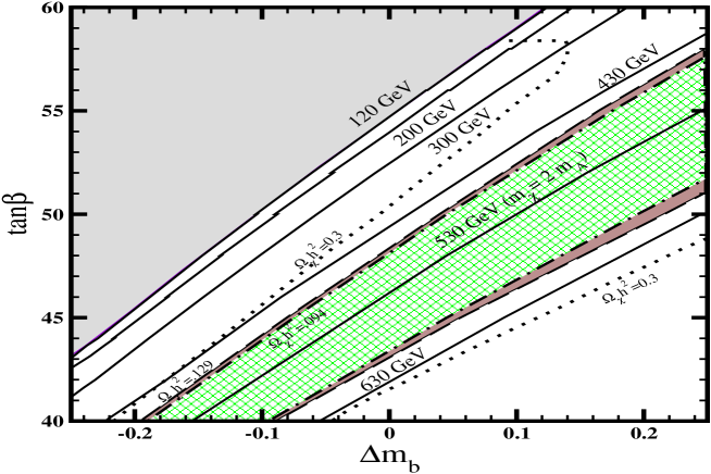
Figure 4: The region allowed by the relic density constraints in the $\tan\beta$ - $\Delta m_{b}$ plane for the case when $m_{0}=m_{\frac{1}{2}}=A_{0}=600$ GeV. Curves with fixed $m_{A}$ are also shown.

3 Sensitivity of Dark Matter to the b Quark Mass without CP Phases

While a considerable body of work already exists on the analyses of supersymmetric dark matter (for a small sample see Ref.([35])), no in depth study exists on the sensitivity of dark matter analyses to the b quark mass. In this section we analyse this sensitivity of the relic density to the b quark mass for the case when the phases are set to zero. In the analysis we use the standard techniques of evolving the parameters given in mSUGRA at the grand unification scale by the renormalization group evolution taking care that charge and color conservation is appropriately preserved (for a recent analysis of charge and color conservation constraints see Ref.[36]). We describe now the result of the analysis. (For a partial previous analysis of this topic see Ref[37]). One of the parameters which enters sensitively in the dark matter analysis is the mass of the CP odd Higgs boson $m_{A}$. Fig. (2) shows $m_{A}$ as a function of the b quark correction $\Delta m_{b}$, which is used as a free parameter. The ranges chosen are such that the $m_{A}$ may lie in the resonance region of the annihilation of the two neutralinos. We find that $m_{A}$ shows a very significant variation as $\Delta m_{b}$ moves in the range $-.3$ to $.3$. Fig. (2) demonstrates the huge sensitivity of $m_{A}$ to the b quark mass. Fig. 2 also shows that for fixed $\tan\beta$ one can enter in the area of the resonance for certain values of $\Delta m_{b}$. Fig. 3 shows the sensitivity of the relic density to corrections to the b quark mass. The analysis was carried out using Micromegas[38]. The dominant channels that contribute to the relic density depend on the mass region and are as follows: In the region $2m_{\chi}\ll m_{A}$ the main channels are $\chi\chi\rightarrow\tau\bar{\tau}$ and $\chi\chi\rightarrow b\bar{b}$. Here typically $\Omega_{\chi}h^{2}>0.5$ and the main contribution comes from t- and u-channel exchange of the sbottom and stau sparticles. Moreover, also the effects of the $\mu$ and $e$ decay channels can be seen. Since their contributions are suppressed by the corresponding slepton masses, it signifies that one is far away from the s-channel Higgs resonances. In the region $2m_{\chi}\sim m_{A}$ the resonant channels account for almost the full contribution to $\Omega_{\chi}h^{2}$ and their influence can be detected several widths, $\Gamma_{A}$, away from the resonance. In this region the contribution to the neutralino relic density from the t- and u-channel exchanges can be as much as 10% within the relic density range allowed by the WMAP data.

Another contribution that can potentially enter is coannihilation. Indeed for $m_{\tilde{\tau}_{1}}<1.25\times m_{\chi}$, one has important effects from $\tilde{\tau}_{1}\chi$ coannihilation. These effects can be observed at the end of the lines of $\Delta m_{b}=10\%,20\%$ in Fig. (3). Thus for low values of $\tan\beta$ one is in the non resonant region and increasing $\tan\beta$ moves one to the resonant region and consequently the relic density decreases due to resonant annihilation. As $\tan\beta$ increases further, the relic density increases to become flat due to the non fermionic decays. Finally, the curves for $\Delta m_{b}$ of $10\%$ and $20\%$ exhibit coannihilation and $\Omega_{\chi}h^{2}$ decreases again due to this effect as $\tan\beta$ increases.

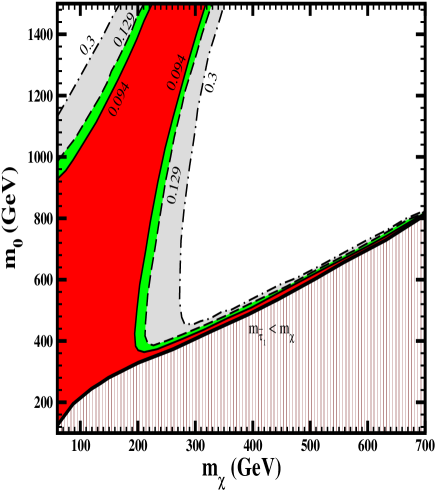
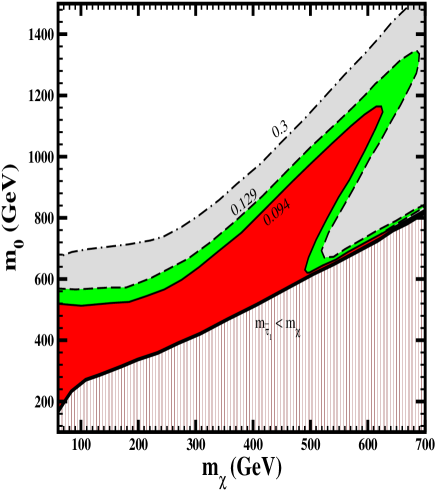
Figure 5: Region in the $m_{0}-m_{\chi}$ plane of mSUGRA allowed by the relic density constraints for the case when $\tan\beta=50$, $|A_{0}|=m_{\frac{1}{2}}$ for values of $\Delta m_{b}=0$ (left) and $\Delta m_{b}=20\%$ (right). The limiting lines close areas such that $\Omega_{\chi}h^{2}$ is below the indicated value.

In Fig.(4) regions with fixed corridors of the relic density are plotted in the $\tan\beta-\Delta m_{b}$ plane. The region consistent with the current range of relic density observed by WMAP is displayed in the dark shaded region. The hatched region has a value of $\Omega_{\chi}h^{2}$ below the WMAP observation. Furthermore, curves with constant values of $m_{A}$ are exhibited. The analysis shows that the region consistent with the WMAP relic density constraint is very sensitive to the $\Delta m_{b}$ correction.

Fig.(5) displays area plots in the $m_{0}-m_{\chi}$ plane of the relic density. The light shaded/grey region has $0.1291<\Omega_{\chi}h^{2}<0.3$. The medium shaded/green region has $0.094<\Omega_{\chi}h^{2}<0.1291$ and is the $2\sigma$ allowed WMAP region. Finally the dark shaded/red region has $\Omega_{\chi}h^{2}<0.094$. The hatched region is excluded as the $\tilde{\tau}$ is the LSP. In Fig.(5) we considered two values of $\Delta m_{b}$; $\Delta m_{b}=0$ and $\Delta m_{b}=20\%$. A comparison of these two exhibits the dramatic dependence of the various regions on the b quark mass. Specifically it is seen that the region consistent with the WMAP constraint is drastically shifted toward lower values of $m_{\chi}/m_{0}$ for smaller $\Delta m_{b}$. Inclusion of the experimental bounds from processes such as $b\rightarrow s\gamma$ on Fig. (5) is beyond the scope of our study. However, the case of $\Delta m_{b}=20\%$ is comparable to the mSUGRA case (where $\Delta m_{b}$ ranges approximately from 17 to 21%). Therefore, the restrictions from the bounds on $b\rightarrow s\gamma$, along with other constraints, on the left graph of Fig. (5) can be approximately deduced from the appropriate figures of Ref. [36].

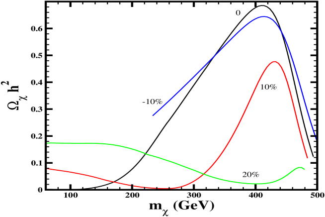
Figure 6: Plot of $\Omega_{\chi}h^{2}$ as a function of $m_{\chi}$ for values of the $\Delta m_{b}$ varying from $(-10\%)-(+20\%)$ when $m_{0}=600$ GeV, $m_{\frac{1}{2}}=|A_{0}|$ and $\tan\beta=50$.

We note that in Fig.(5) there is a region where $m_{0}$ and $m_{\frac{1}{2}}$ get large and appear to have a superficial resemblance with the Hyperbolic Branch/Focus Point (HB/FP) region[11]. However, the mechanism by which relic density constraint is satisfied in the WMAP region is entirely different in this case than in the HB/FP case[39, 40]. Thus in the analysis presented here the relic density constraints are satisfied by the mechanism of proximity to a resonant state (see also in this context Ref.[41]) while for the HB/FP region the satisfaction occurs with a significant amount of coannihilation. In Fig.(6) we give a plot of $\Omega_{\chi}h^{2}$ as a function of $m_{\chi}$ for fixed $m_{0}$ (i.e., $m_{0}=600$ GeV) and $\tan\beta=50$ for $\Delta m_{b}$ values varying in the range $(-10\%)-(+20\%)$. Again one finds that the relic density is sharply dependent on the b quark mass correction.

4 Sensitivity of Dark Matter to the b Quark Mass with CP Phases

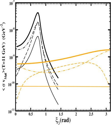
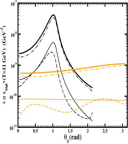
Figure 7: A plot of $\langle\sigma v_{\rm{Mo\!\!\!/l}}\rangle$ as a function of $\xi_{3}$ and $\theta_{\mu}$ (with the other phases set to zero) for the case when $m_{0}=m_{\frac{1}{2}}=A_{0}=600$ GeV, $\tan\beta=50$ and using the theoretically predicted value of $\Delta m_{b}$ (black lines), $\Delta m_{b}=0$ (light lines). The contribution of dominant channels to $\langle\sigma v_{\rm{Mo\!\!\!/l}}\rangle$ are also shown: all contributions (thick lines), only s-channel $H_{1}$ mediated annihilation to $b\bar{b}$ (dashed lines) and only s-channel $H_{3}$ mediated annihilation to $b\bar{b}$ (dot-dashed lines) and all s-channel annihilation to $\tau\bar{\tau}$ (solid thin lines).

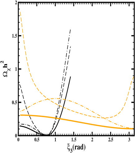
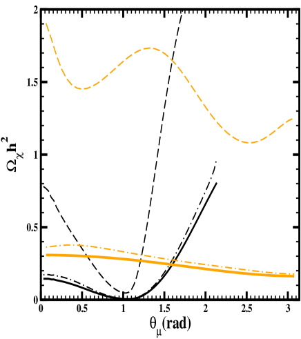
Figure 8: A plot of the neutralino relic density $\Omega_{\chi}h^{2}$ as a function of $\xi_{3}$ and $\theta_{\mu}$ for $m_{0}=m_{\frac{1}{2}}=A_{0}=600$ GeV, $\tan\beta=50$ and using the theoretically predicted value of $\Delta m_{b}$ (black lines), $\Delta m_{b}=0$ (light lines). The contribution of dominant s-channels to the relic density are represented by the same type of lines as fig. (7).

We now give the analysis with inclusion of CP phases. In the calculation of the relic density, we only consider the contribution from the s-channel exchange of the three Higgs $H_{1},H_{2},H_{3}$ and the t- and u-channel exchange of sfermions as shown in Fig.1. The prediction for the Higgs masses and widths are extracted from the newly developed software package CPsuperH[42]. The impact of the CP phases on the relic density is as in the case without CP phases, i.e., mainly through $\Delta m_{b}$. On the other hand the effects of the Higgs mixing are marginal. In Fig. (7) we give a plot of the thermally averaged annihilation cross-section at a temperature of the order of the freeze out temperature $T_{f}$ (see Eq.(40) of the Appendix) as a function of $\theta_{\mu}$ and $\xi_{3}$ for $\tan\beta=50$. The contribution of individual channels are also displayed. The channels with the $b\bar{b}$ final state dominate over the channels with $\tau\bar{\tau}$ final state due to the color factor. We plot $\Omega_{\chi}h^{2}$ as a function of $\theta_{\mu}$ and $\xi_{3}$ in Fig. (8) for the same case. Figs. (7) and (8) also exhibit the dependence on the bottom mass correction, as two different values are used; the theoretical value of $\Delta m_{b}$ (black lines) and $\Delta m_{b}=0$ (light lines). The large effects of CP phases on the relic density in this case are clearly evident. In particular it is seen that the largest impact from the CP phases arises from their influence on the value of $\Delta m_{b}$. The curves with $\Delta m_{b}$ confined to a constant vanishing value show less variations with the CP phases, although $\Omega_{\chi}h^{2}$ still changes by almost a factor of two due to the variation of the Higgs couplings. The large effect of the $\Delta m_{b}$ arises via its effect on $m_{A}$. Similar plots as functions of $\xi_{3}$ are given in Fig. (9) for $\tan\beta=40$.

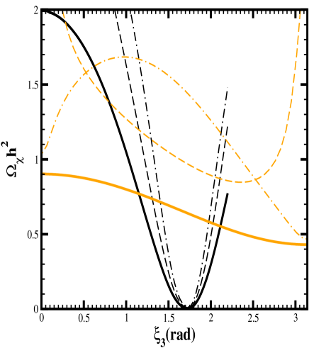
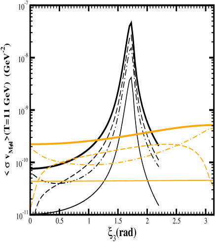
Figure 9: Same as Fig. (7) and Fig. (8) for $\tan\beta=40$.

Case	$|d_{e}|e.cm$	$|d_{n}|e.cm$	$C_{Hg}cm$
(i)	$2.74\times 10^{-27}$	$1.79\times 10^{-26}$	$8.72\times 10^{-27}$
(ii)	$1.29\times 10^{-27}$	$1.82\times 10^{-27}$	$6.02\times 10^{-28}$
(iii)	$9.72\times 10^{-28}$	$4.19\times 10^{-26}$	$1.41\times 10^{-27}$

Table 1: The EDMs for $\tan\beta=40$ for cases (i)-(iii) of text.

The dependence of the neutralino relic density on $\alpha_{A_{0}}$ is displayed in Fig. (10). This dependence arises from the effect of $\alpha_{A_{0}}$ on $m_{\tilde{\tau_{1}}}$ and $m_{A}$. Thus for fixed $A_{0}$, variations in $\alpha_{A_{0}}$ affect $m_{\tilde{\tau_{1}}}$ which can generate $\tilde{\tau}\chi$ coannihilations, and even push $m_{\tilde{\tau}_{1}}$ below $m_{\chi}$.

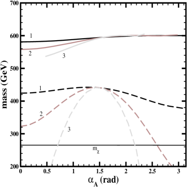
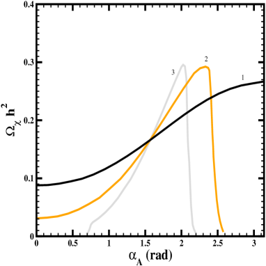
Figure 10: The left graph shows the dependence of $m_{A}$ (solid lines) and $m_{\tilde{\tau_{1}}}$ (dashed lines) on $\alpha_{A_{0}}$ for $m_{0}=m_{\frac{1}{2}}=600$ GeV, $\tan\beta=50$ and for three different values of $|A_{0}|/m_{\frac{1}{2}}$ (indicated on the curves). The neutralino relic density for the same three cases is displayed in the graph on the right.

In Fig. (11) the neutralino relic density is displayed as a function of $\tan\beta$ for three cases given by: (i) $m_{0}=m_{1/2}$=$|A_{0}|=300$ GeV, $\alpha_{A_{0}}=1.0$, $\xi_{1}=0.5$, $\xi_{2}=0.66$, $\xi_{3}=0.62$, $\theta_{\mu}=2.5$; (ii) $m_{0}=m_{1/2}=|A_{0}|=555$ GeV, $\alpha_{A_{0}}=2.0$, $\xi_{1}=0.6$, $\xi_{2}=0.65$, $\xi_{3}=0.65$, $\theta_{\mu}=2.5$; (iii) $m_{0}=m_{1/2}=|A_{0}|=480$ GeV, $\alpha_{A_{0}}=0.8$, $\xi_{1}=0.4$, $\xi_{2}=0.66$, $\xi_{3}=0.63$, $\theta_{\mu}=2.5$. In all cases the EDM constraints for the electron, the neutron and for ${}^{199}Hg$ are satisfied for $\tan\beta=40$ and their values are exhibited in table 1. These results may be compared with the current experimental limits on the EDM of the electon, the neutron and on ${}^{199}Hg$ as follows: $|d_{e}|<4.23\times 10^{-27}ecm$, $|d_{n}|<6.5\times 10^{-26}ecm$ and $C_{\rm Hg}<3.0\times 10^{-26}cm$ from the ¹⁹⁹Hg analysis (where $C_{\rm Hg}$ is defined as in Ref. [25]).

Figure 11: The neutralino relic density as a function of $\tan\beta$ for the three cases (i), (ii), (iii) of the text. Lines (I), (II) and (III) correspond to similar set of SUSY parameters for the case of vanishing phases.

From Fig. (3) and Fig. (4) it is apparent that larger negative corrections to the bottom quark mass push the resonance region toward smaller values of $\tan\beta$. Use of nonuniversalities for the gaugino masses, including the case of having relative signs among them, allows for larger negative corrections to the b quark mass. Therefore, it is possible to achieve agreement with the WMAP result for lower values of $\tan\beta$ than in the mSUGRA case. Considering only the main contributions from the gluino-sbottom, the bottom quark mass correction will reach its maximum negative value for $\theta_{\mu}+\xi_{3}=\pi$. The phase of the trilinear coupling also plays a role through the chargino loop. Thus we investigate the case with $\theta_{\mu}=0$, $\xi_{3}=\pi$, and take $\alpha_{A_{0}}=\pi$ at the GUT scale. As an illustration we show in Fig.(12) that indeed the WMAP result is compatible with $\tan\beta=30$ in the resonant s-channel region. The analysis also implies that the upper limit on the neutralino mass will be larger than in the mSUGRA case. For $\tan\beta=30$ we find an upper bound of $\sim 700$ GeV, as seen in Fig. (12). For comparison the upper bound in mSUGRA is found to be 500 GeV for $\tan\beta<30$ in Ref.[39].

Figure 12: The neutralino relic density as a function of the lightest neutralino mass for $\tan\beta=30$, $\xi_{1}=0$, $\xi_{2}=0$, $\xi_{3}=\pi$, $\alpha_{A_{0}}=\pi$ and $\theta_{\mu}=0$. Two different values of $m_{0}$ are displayed: (i) $m_{0}=600$ GeV (solid line) and (ii) $m_{0}=750$ GeV (dashed line).

5 Conclusion

In this paper we have carried out a detailed analysis to study the sensitivity of dark matter to the b quark mass. This is done in two ways: by assuming that the correction to the b quark mass in a free parameter and also computing it from loop corrections. In each case it is found that the relic density is very sensitive to the mass of the b quark for large $\tan\beta$. In the analysis we focus on the region where the relic density constraints are satisfied by annihilation through resonant Higgs poles. The analysis is then extended to include CP phases in the soft parameters taking account of the CP-even and CP-odd Higgs mixing. Sensitivity of the relic density to variations in the b quark mass and to CP phases are then investigated and a great sensitivity to variations in the b quark mass with inclusion of phases in again observed. These results have important implications for predictions of dark matter in models where $\tan\beta$ is large, such as in unified models bases on $SO(10)$, and for the observation of supersymmetric dark matter in such models.

Acknowledgments
MEG acknowledges support from the ‘Fundacão para a Ciência e Tecnologia’ under contract SFRH/BPD/5711/2001, the ’Consejería de Educación de la Junta de Andalucía’ and the Spanish DGICYT under contract BFM2003-01266. The research of TI and PN was supported in part by NSF grant PHY-0139967. SS acknowledges support from the European RTN network HPRN-CT-2000-00148.

APPENDIX A: Relic Density Analysis
The analysis of neutralino relic density must be done with care since one has direct channel poles and one must use the accurate method on doing the thermal averaging over these poles[43]. We give here the basic formulas for the relic density analysis[43, 44, 45]

$$\Omega_{\chi}h^{2}=2.755\;\ 10^{8}\times\frac{m_{\chi}}{{\rm GeV}}Y_{0}.$$ (37)

The evolution equation for $Y$ is given by

$$\frac{dY}{dT}=\sqrt{\frac{\pi g_{*}(T)}{45G}}\langle\sigma v_{\rm{Mo\!\!\!/l}}\rangle(Y^{2}-Y_{eq}^{2}),$$ (38)

Here $\langle\sigma v_{\rm{Mo\!\!\!/l}}\rangle$ is the thermal average of the neutralino annihilation cross section multiplied by the Møller velocity [44], $Y_{0}=Y(T=T_{0}=2.726K)$, where $T_{0}$ is the microwave background temperature, $Y_{\rm eq}=Y_{\rm eq}(T)$ is the thermal equilibrium abundance given by

$$Y_{\rm eq}(T)=2\times\frac{45}{4\pi^{4}h_{\rm eff}(T)}\left(\frac{m_{\chi}}{T}\right)^{2}K_{2}(\frac{m_{\chi}}{T}).$$ (39)

The number of degrees of freedom is $g_{*}\sim 81$. However, we use a more precise value as a function of the temperature obtained from Ref. [46] and the same is done for $h_{\rm eff}$. To calculate the freeze-out temperature $T_{f}$ we use the relation

$$\frac{d\ln(Y_{\rm eq})}{dT}=\sqrt{\frac{\pi g_{*}(T)}{45G}}\langle\sigma v_{\rm{Mo\!\!\!/l}}\rangle Y_{\rm eq}\delta(\delta+2)$$ (40)

The equation for $Y_{0}$ is

$$\frac{1}{Y_{0}}=\frac{1}{Y_{f}}+X_{T_{f}}$$ (41)

and $Y_{f}=Y(T_{F})=(1+\delta)Y_{\rm eq}(T_{f})$. We have introduced the amount $X_{T_{f}}$ such that we can split the independent contribution of each channel

$$X_{T_{f}}=\sqrt{\frac{\pi}{45G}}\int^{T_{f}}_{T_{0}}g_{*}(T)^{1/2}\langle\sigma v_{\rm{Mo\!\!\!/l}}\rangle dT$$ (42)

We have taken $T_{0}=0$ and $\delta=1.5$ following the suggestion of Micromegas. As stated already care must be taken in computing thermal averaging since one must integrate over the direct channel poles properly [43]. We use the relation

$$\langle\sigma v_{\rm{Mo\!\!\!/l}}\rangle(T)=\frac{1}{8m_{\chi}^{4}TK_{2}^{2}(m_{\chi}/T)}\int^{\infty}_{4m_{\chi}^{2}}ds\sigma(s)(s-4m_{\chi}^{2})\sqrt{s}K_{1}\left(\frac{\sqrt{s}}{T}\right)$$ (43)

To calculate $\sigma(s)$ from the partial amplitudes we use the following definitions

$$\sigma(s)=2w(s)/\sqrt{s(s-4m_{\chi}^{2})}$$ (44)

Since we only consider channels $\chi\chi\rightarrow f\bar{f}$, ($f=b,\tau$), $w(s)$ becomes,

$$w(s)=\frac{1}{32\pi}\sum_{f=b,\tau}c_{f}\times(1-\frac{4m_{f}^{2}}{s})\tilde{w}_{f}(s)$$ (45)

$c_{f}$ is the color factor so that $c_{b}=3$, $c_{\tau}=1$. The definition of $\tilde{w}_{f}(s)$ is directly related to the amplitude

$$\tilde{w}_{f}(s)=\frac{1}{2}\int_{-1}^{1}dcos\theta_{CM}|A(\chi\chi\rightarrow f\bar{f})|^{2}$$ (46)

References

- [1] C. L. Bennett et al., Astrophys. J. Suppl. 148, 1 (2003) [arXiv:astro-ph/0302207].
- [2] D. N. Spergel et al., Astrophys. J. Suppl. 148, 175 (2003) [arXiv:astro-ph/0302209].
- [3] R. Belli et.al., Phys. Lett.B480,23(2000), ”Search for WIMP annual modulation signature: results from DAMA/NAI-3 and DAMA/NAI-4 and the global combined analysis”, DAMA collaboration preprint INFN/AE-00/01, 1 February, 2000.
- [4] L. Baudis, A. Dietz, B. Majorovits, F. Schwamm, H. Strecker and H.V. Klapdor-Kleingrothaus, Phys. Rev. D63,022001 (2001).
- [5] A. Benoit et al., Phys. Lett. B 545, 43 (2002) [arXiv:astro-ph/0206271].
- [6] H.V. Klapdor-Kleingrothaus, et.al., ”GENIUS, A Supersensitive Germanium Detector System for Rare Events: Proposal”, MPI-H-V26-1999, hep-ph/9910205.
- [7] D. Cline et al., “A Wimp Detector With Two-Phase Xenon,” Astropart. Phys. 12, 373 (2000).
- [8] A.H. Chamseddine, R. Arnowitt and P. Nath, Phys. Rev. Lett. 49, 970 (1982); R. Barbieri, S. Ferrara and C.A. Savoy, Phys. Lett. B 119, 343 (1982); L. Hall, J. Lykken, and S. Weinberg, Phys. Rev. D 27, 2359 (1983): P. Nath, R. Arnowitt and A.H. Chamseddine, Nucl. Phys. B 227, 121 (1983). For a recent review see, P. Nath, “Twenty years of SUGRA,” arXiv:hep-ph/0307123.
- [9] H. Goldberg, Phys. Rev. Lett. 50, 1419 (1983); J. R. Ellis, J. S. Hagelin, D. V. Nanopoulos, K. A. Olive and M. Srednicki, Nucl. Phys. B 238, 453 (1984).
- [10] T. Ibrahim and P. Nath, Phys. Rev. D 58, 111301 (1998).
- [11] K.L. Chan, U. Chattopadhyay and P. Nath, Phys. Rev. D 58, 096004 (1998). J. L. Feng, K. T. Matchev and T. Moroi, Phys. Rev. D 61, 075005 (2000).
- [12] L. J. Hall, R. Rattazzi and U. Sarid, Phys. Rev. D 50, 7048 (1994). M. Carena, M. Olechowski, S. Pokorski and C. E. Wagner, Nucl. Phys. B 426, 269 (1994). D. M. Pierce, J. A. Bagger, K. T. Matchev and R. j. Zhang, Nucl. Phys. B 491, 3 (1997).
- [13] T. Ibrahim and P. Nath, Phys. Rev. D 67, 095003 (2003) [arXiv:hep-ph/0301110].
- [14] T. Ibrahim and P. Nath, Phys. Rev. D 68, 015008 (2003) [arXiv:hep-ph/0305201].
- [15] T. Ibrahim and P. Nath, arXiv:hep-ph/0311242 (to appear in Phys. Rev. D).
- [16] M.E. Gomez, G. Lazarides and C. Pallis, Phys. Rev. D61, 123512 (2000); Phys. Lett. B 487, 313 (2000); Nucl. Phys. B 638, 165 (2002) [arXiv:hep-ph/0203131]; Phys. Rev. D 67, 097701 (2003); C. Pallis and M. E. Gomez, arXiv:hep-ph/0303098.
- [17] H. Baer and J. Ferrandis, Phys. Rev. Lett. 87, 211803 (2001) [arXiv:hep-ph/0106352]; T. Blazek, R. Dermisek and S. Raby, Phys. Rev. Lett. 88, 111804 (2002) [arXiv:hep-ph/0107097]; U. Chattopadhyay, A. Corsetti and P. Nath, Phys. Rev. D 66, 035003 (2002) [arXiv:hep-ph/0201001]; U. Chattopadhyay and P. Nath, Phys. Rev. D 65, 075009 (2002) [arXiv:hep-ph/0110341]; S. Mizuta and M. Yamaguchi, Phys. Lett. B 298, 120 (1993) [arXiv:hep-ph/9208251]; K. Tobe and J. D. Wells, Nucl. Phys. B 663, 123 (2003) [arXiv:hep-ph/0301015].
- [18] M. E. Gomez and J. D. Vergados, Phys. Lett. B 512, 252 (2001); J. R. Ellis, T. Falk, G. Ganis, K. A. Olive and M. Srednicki, Phys. Lett. B 510, 236 (2001); R. Arnowitt, B. Dutta and Y. Santoso, Nucl. Phys. B 606, 59 (2001)
- [19] E. Commins, et. al., Phys. Rev. A50, 2960(1994).
- [20] P.G. Harris et.al., Phys. Rev. Lett. 82, 904(1999).
- [21] S. K. Lamoreaux, J. P. Jacobs, B. R. Heckel, F. J. Raab and E. N. Fortson, Phys. Rev. Lett. 57, 3125 (1986).
- [22] The edm constraints may be improved further by measurement of the deutron edm. See, e.g., O. Lebedev, K. A. Olive, M. Pospelov and A. Ritz, arXiv:hep-ph/0402023.
- [23] P. Nath, Phys. Rev. Lett.66, 2565(1991); Y. Kizukuri and N. Oshimo, Phys.Rev.D46,3025(1992).
- [24] T. Ibrahim and P. Nath, Phys. Lett. B 418, 98 (1998); Phys. Rev. D57, 478(1998); T. Falk and K Olive, Phys. Lett. B 439, 71(1998); M. Brhlik, G.J. Good, and G.L. Kane, Phys. Rev. D59, 115004 (1999); A. Bartl, T. Gajdosik, W. Porod, P. Stockinger, and H. Stremnitzer, Phys. Rev. 60, 073003(1999); S. Pokorski, J. Rosiek and C.A. Savoy, Nucl.Phys. B570, 81(2000); E. Accomando, R. Arnowitt and B. Dutta, Phys. Rev. D 61, 115003 (2000); U. Chattopadhyay, T. Ibrahim, D.P. Roy, Phys.Rev.D64:013004,2001; C. S. Huang and W. Liao, Phys. Rev. D 61, 116002 (2000); ibid, Phys. Rev. D 62, 016008 (2000); A.Bartl, T. Gajdosik, E.Lunghi, A. Masiero, W. Porod, H. Stremnitzer and O. Vives, hep-ph/010332; M. Brhlik, L. Everett, G. Kane and J. Lykken, Phys. Rev. Lett. 83, 2124, 1999; Phys. Rev. D62, 035005(2000); E. Accomando, R. Arnowitt and B. Datta, Phys. Rev. D61, 075010(2000); T. Ibrahim and P. Nath, Phys. Rev. D61, 093004(2000).
- [25] T. Falk, K.A. Olive, M. Prospelov, and R. Roiban, Nucl. Phys. B560, 3(1999); V. D. Barger, T. Falk, T. Han, J. Jiang, T. Li and T. Plehn, Phys. Rev. D 64, 056007 (2001); S.Abel, S. Khalil, O.Lebedev, Phys. Rev. Lett. 86, 5850(2001); T. Ibrahim and P. Nath, Phys. Rev. D 67, 016005 (2003)
- [26] D. Chang, W-Y.Keung,and A. Pilaftsis, Phys. Rev. Lett. 82, 900(1999).
- [27] K.S. Babu, B. Dutta and R. N. Mohapatra, Phys. Rev. D61, 091701(2000).
- [28] A. Pilaftsis, Phys. Rev. D58, 096010; Phys. Lett.B435, 88(1998); A. Pilaftsis and C.E.M. Wagner, Nucl. Phys. B553, 3(1999); D.A. Demir, Phys. Rev. D60, 055006(1999); S. Y. Choi, M. Drees and J. S. Lee, Phys. Lett. B 481, 57 (2000); M. Boz, Mod. Phys. Lett. A 17, 215 (2002).
- [29] T. Ibrahim and P. Nath, Phys.Rev.D63:035009,2001; hep-ph/0008237; T. Ibrahim, Phys. Rev. D 64, 035009 (2001);
- [30] T. Ibrahim and P. Nath, Phys. Rev. D 66, 015005 (2002); S. W. Ham, S. K. Oh, E. J. Yoo, C. M. Kim and D. Son, arXiv:hep-ph/0205244.
- [31] M. Carena, J. R. Ellis, A. Pilaftsis and C. E. Wagner, Nucl. Phys. B 625, 345 (2002) [arXiv:hep-ph/0111245]. ; M. Carena, J. Ellis, S. Mrenna, A. Pilaftsis and C. E. Wagner, arXiv:hep-ph/0211467.
- [32] U. Chattopadhyay, T. Ibrahim and P. Nath, Phys. Rev. D60,063505(1999); T. Falk, A. Ferstl and K. Olive, Astropart. Phys. 13, 301(2000); S. Khalil, Phys. Lett. B484, 98(2000); S. Khalil and Q. Shafi, Nucl.Phys. B564, 19(1999); K. Freese and P. Gondolo, hep-ph/9908390; S.Y. Choi, hep-ph/9908397.
- [33] H. Arason, D.J. Castano, B.E. Kesthelyi, S. Mikaelian, E.J. Piard, P. Ramond, and B.D. Wright, Phys. Rev. Lett. 67, 2933(1991); D. Pierce, J. Bagger, K. Matchev and R. Zhang, Nucl. Phys. B491, 3(1997)
- [34] M. Carena and H. E. Haber, Prog. Part. Nucl. Phys. 50, 63 (2003) [arXiv:hep-ph/0208209].
- [35] K. Greist, Phys. Rev. D38, 2357(1988); J. Ellis and R. Flores, Nucl. Phys. B307, 833(1988); R. Barbieri, M. Frigeni and G. Giudice, Nucl. Phys. B313, 725(1989); A. Bottino et.al., B295, 330(1992); M. Drees and M.M. Nojiri, Phys. Rev.D48,3483(1993); V.A. Bednyakov, H.V. Klapdor-Kleingrothaus and S. Kovalenko, Phys. Rev.D50, 7128(1994); P. Nath and R. Arnowitt, Phys. Rev. Lett. 74, 4592(1995); R. Arnowitt and P. Nath, Phys. Rev. D54, 2374(1996); E. Diehl, G.L. Kane, C. Kolda, J.D. Wells, Phys.Rev.D52, 4223(1995); L. Bergstrom and P. Gondolo, Astrop. Phys. 6, 263(1996); H. Baer and M. Brhlik, Phys.Rev.D57,567(1998); J.D. Vergados, Phys. Rev. D83, 3597(1998); J.L. Feng, K. T. Matchev, F. Wilczek, Phys.Lett. B482, 388(2000); M. Brhlik, D. J. Chung and G. L. Kane, Int. J. Mod. Phys. D 10, 367 (2001); V.A. Bednyakov and H.V. Klapdor-Kleingrothaus, Phys. Rev. D 63, 095005 (2001); M. E. Gomez and J. D. Vergados, Phys. Lett. B 512, 252 (2001); A. Corsetti and P. Nath, Phys. Rev. D 64, 125010 (2001); A. B. Lahanas, D. V. Nanopoulos and V. C. Spanos, Phys. Lett. B 518, 94 (2001); J.L. Feng, K. T. Matchev, F. Wilczek, Phys. Rev. D 63, 045024 (2001); V. D. Barger and C. Kao, Phys. Lett. B 518, 117 (2001).
- [36] D. G. Cerdeno, E. Gabrielli, M. E. Gomez and C. Munoz, JHEP 0306, 030 (2003) [arXiv:hep-ph/0304115].
- [37] J. R. Ellis, K. A. Olive, Y. Santoso and V. C. Spanos, arXiv:hep-ph/0310356.
- [38] G. Belanger, F. Boudjema, A. Pukhov and A. Semenov, Comput. Phys. Commun. 149, 103 (2002) [arXiv:hep-ph/0112278]. For an analysis of uncertainties in the determination of relic density in different public codes see, B. C. Allanach, G. Belanger, F. Boudjema, A. Pukhov and W. Porod, hep-ph/0402161.
- [39] J. R. Ellis, K. A. Olive, Y. Santoso and V. C. Spanos, Phys. Lett. B 565, 176 (2003) [arXiv:hep-ph/0303043].
- [40] H. Baer and C. Balazs, JCAP 0305, 006 (2003) [arXiv:hep-ph/0303114].; U. Chattopadhyay, A. Corsetti and P. Nath, Phys. Rev. D 68, 035005 (2003) [arXiv:hep-ph/0303201]; H. Baer, C. Balazs, A. Belyaev, T. Krupovnickas and X. Tata, JHEP 0306, 054 (2003) [arXiv:hep-ph/0304303]; A. B. Lahanas and D. V. Nanopoulos, Phys. Lett. B 568, 55 (2003) [arXiv:hep-ph/0303130]; H. Baer, T. Krupovnickas and X. Tata, JHEP 0307, 020 (2003) [arXiv:hep-ph/0305325]; A. B. Lahanas, N. E. Mavromatos and D. V. Nanopoulos, Int. J. Mod. Phys. D 12, 1529 (2003) [arXiv:hep-ph/0308251].
- [41] H. Baer and J. O’Farrill, arXiv:hep-ph/0312350.
- [42] J.S. Lee, A. Pilaftsis, M. Carena, S.Y. Choi, M. Drees, J. Ellis, C.E.M. Wagner, Comput.Phys.Commun. 156 (2004) 283-317.
- [43] K. Greist and D. Seckel, Phys. Rev. D43, 3191(1991); R. Arnowitt and P. Nath, Phys. Lett. B299, 103(1993); Phys. Rev. Lett. 70, 3696(1993); H. Baer and M. Brhlik, Phys. Rev. D53, 597(1996); V. Barger and C. Kao, Phys. Rev. D57, 3131(1998).
- [44] P. Gondolo and G. Gelmini, Nucl. Phys. B360, 145(1991).
- [45] T. Nihei, L. Roszkowski and R. Ruiz de Austri, JHEP 0203, 031 (2002) [arXiv:hep-ph/0202009].
- [46] P. Gondolo, J. Edsjo, P. Ullio, L. Bergstrom, M. Schelke and E. A. Baltz, arXiv:astro-ph/0211238. http://www.physto.se/ edsjo/darksusy/