Isomeric Lepton Mass Matrices and Bi-large Neutrino Mixing

Abstract

We show that there exist six parallel textures of the charged lepton and neutrino mass matrices with six vanishing entries, whose phenomenological consequences are exactly the same. These isomeric lepton mass matrices are compatible with current experimental data at the $3\sigma$ level. If the seesaw mechanism and the Fukugita-Tanimoto-Yanagida hypothesis are taken into account, it will be possible to fit the experimental data at or below the $2\sigma$ level. In particular, the maximal atmospheric neutrino mixing can be reconciled with a strong neutrino mass hierarchy in the seesaw case.

The recent solar [1], atmospheric [2], KamLAND [3] and K2K [4] neutrino oscillation experiments have provided us with very convincing evidence that neutrinos are massive and lepton flavors are mixed. In particular, the admixture of three lepton flavors involves two large angles $\theta_{12}\sim 33^{\circ}$ and $\theta_{23}\sim 45^{\circ}$ [5]. To interpret the observed bi-large lepton flavor mixing pattern, many phenomenological ans$\rm\ddot{a}$tze of lepton mass matrices have been proposed in the literature [6]. A very interesting category of the ans$\rm\ddot{a}$tze focus on texture zeros of charged lepton and neutrino mass matrices in a specific flavor basis, from which some nontrivial and testable relations between flavor mixing angles and lepton mass ratios can be derived. A typical example is the Fritzsch ansatz [7] of lepton mass matrices,

$$M^{~{}}_{l,\nu}\;=\;\left(\matrix{{\bf 0}&\times&{\bf 0}\cr\times&{\bf 0}&\times\cr{\bf 0}&\times&\times\cr}\right)\;,$$ (1)

in which six texture zeros are included and all non-vanishing entries are simply symbolized by $\times$’s. It has been shown in Ref. [8] that this ansatz can naturally predict a normal but weak neutrino mass hierarchy and a bi-large lepton flavor mixing pattern. If the seesaw mechanism is incorporated in the Fritzsch texture of charged lepton and Dirac neutrino mass matrices [9], one may obtain a similar flavor mixing pattern together with a much stronger neutrino mass hierarchy.

The simplicity and predictability of $M_{l}$ and $M_{\nu}$ in Eq. (1) motivate us to examine other possible six-zero textures of lepton mass matrices and their various phenomenological consequences. We find that there totally exist six parallel patterns of $M_{l}$ and $M_{\nu}$ with six texture zeros, as listed in Table 1, where the Fritzsch ansatz is labelled as pattern (A). It is apparent that these six patterns are structurally different from one another. The question is whether their predictions for neutrino masses, flavor mixing angles and CP violation are distinguishable or not.

The purpose of this paper is to answer the above question and to confront those six-zero textures of lepton mass matrices with the latest experimental data. First, we shall present a concise analysis of the lepton mass matrices in Table 1 and reveal their isomeric features – namely, they have the same phenomenological consequences, although their structures are apparently different. Second, we shall examine the predictions of these lepton mass matrices by comparing them with the $2\sigma$ and $3\sigma$ intervals of two neutrino mass-squared differences and three lepton flavor mixing angles [10], which are obtained from a global analysis of the latest solar, atmospheric, reactor (KamLAND and CHOOZ [11]) and accelerator (K2K) neutrino data. We find no parameter space allowed for six isomeric lepton mass matrices at the $2\sigma$ level. At the $3\sigma$ level, however, their results for neutrino masses and lepton flavor mixing angles can be compatible with current data. Third, we incorporate the seesaw mechanism and the Fukugita-Tanimoto-Yanagida hypothesis [9] in the charged lepton and Dirac neutrino mass matrices with six texture zeros. It turns out that their predictions, including $\theta_{23}\approx 45^{\circ}$, are in good agreement with the present experimental data even at the $2\sigma$ level.

Let us begin with the diagonalization of $M_{l}$ and $M_{\nu}$ listed in Table 1. Without loss of generality, one may take their diagonal non-vanishing elements to be real and positive. Then only the off-diagonal non-vanishing elements of $M_{l}$ and $M_{\nu}$ are complex. Each mass matrix $M$ consists of two phase parameters ($\phi$ and $\varphi$) and three real and positive parameters ($A$, $B$ and $C$), as shown in Table 1, where their subscript “$l$” or “$\nu$” has been omitted for simplicity. The diagonalization of $M$ requires the following unitary transformation,

$$U^{\dagger}MU^{*}\;=\;\left(\matrix{\lambda_{1}&0&0\cr 0&\lambda_{2}&0\cr 0&0&\lambda_{3}\cr}\right)\;,$$ (2)

where $\lambda_{i}$ (for $i=1,2,3$) denote the physical masses of charged leptons (i.e., $\lambda_{1,2,3}=m_{e,\mu,\tau}$) or neutrinos (i.e., $\lambda_{i}=m_{i}$). Due to the particular texture of $M$, $U$ can be written as a product of a diagonal phase matrix (dependent on $\phi$ and $\varphi$) and a unitary matrix (independent of $\phi$ and $\varphi$), as illustrated by Table 1. The real parameters $(A,B,C)$ in $M$ and $(a^{~{}}_{i},b^{~{}}_{i},c^{~{}}_{i})$ in $U$ are simple functions of $\lambda_{i}$:

$$A = \lambda_{3}\left(1-y+xy\right)\;,$$ (3)

$$B = \lambda_{3}\left[\frac{y(1-x)(1-y)(1+xy)}{1-y+xy}\right]^{1/2}\;,$$ (4)

$$C = \lambda_{3}\left(\frac{xy^{2}}{1-y+xy}\right)^{1/2}\;;$$ (5)

and

$$a^{~{}}_{1} = +\left[\frac{1-y}{(1+x)(1-xy)(1-y+xy)}\right]^{1/2}\;,$$ (6)

$$a^{~{}}_{2} = -i\left[\frac{x(1+xy)}{(1+x)(1+y)(1-y+xy)}\right]^{1/2}\;,$$ (7)

$$a^{~{}}_{3} = +\left[\frac{xy^{3}(1-x)}{(1-xy)(1+y)(1-y+xy)}\right]^{1/2}\;,$$ (8)

$$b^{~{}}_{1} = +\left[\frac{x(1-y)}{(1+x)(1-xy)}\right]^{1/2}\;,$$ (9)

$$b^{~{}}_{2} = +i\left[\frac{1+xy}{(1+x)(1+y)}\right]^{1/2}\;,$$ (10)

$$b^{~{}}_{3} = +\left[\frac{y(1-x)}{(1-xy)(1+y)}\right]^{1/2}\;,$$ (11)

$$c^{~{}}_{1} = -\left[\frac{xy(1-x)(1+xy)}{(1+x)(1-xy)(1-y+xy)}\right]^{1/2}\;,$$ (12)

$$c^{~{}}_{2} = -i\left[\frac{y(1-x)(1-y)}{(1+x)(1+y)(1-y+xy)}\right]^{1/2}\;,$$ (13)

$$c^{~{}}_{3} = +\left[\frac{(1-y)(1+xy)}{(1-xy)(1+y)(1-y+xy)}\right]^{1/2}\;,$$ (14)

where $x\equiv\lambda_{1}/\lambda_{2}$ and $y\equiv\lambda_{2}/\lambda_{3}$ have been defined. Note that $a^{~{}}_{2}$, $b^{~{}}_{2}$ and $c^{~{}}_{2}$ are imaginary, and their nontrivial phases arise from a minus sign of the determinant of $M$(i.e., ${\rm Det}(M)=-AC^{2}e^{2i\varphi}$). Since the charged lepton masses have precisely been measured [12], we have $x^{~{}}_{l}\approx 0.00484$ and $y^{~{}}_{l}\approx 0.0594$. On the other hand, $0<x_{\nu}<1$ is required by the solar neutrino oscillation data [1]. Hence $0<y_{\nu}<1$ must hold, in agreement with Eq. (4). This observation implies that the isomeric lepton mass matrices under discussion guarantee a normal neutrino mass spectrum.

The lepton flavor mixing matrix $V$, which links the neutrino mass eigenstates $(\nu_{1},\nu_{2},\nu_{3})$ to the neutrino flavor eigenstates $(\nu_{e},\nu_{\mu},\nu_{\tau})$, results from the mismatch between the diagonalization of $M_{l}$ and that of $M_{\nu}$. Taking account of Eq. (2), we obtain $V=U^{\dagger}_{l}U_{\nu}$, whose nine matrix elements read explicitly as

$$V_{pq}\;=\;(a^{l}_{p})^{*}a^{\nu}_{q}e^{i\alpha}+(b^{l}_{p})^{*}b^{\nu}_{q}e^{i\beta}+(c^{l}_{p})^{*}c^{\nu}_{q}\;,$$ (15)

where the subscripts $p$ and $q$ run respectively over $(e,\mu,\tau)$ and $(1,2,3)$, and the phase parameters $\alpha$ and $\beta$ are defined by $\alpha\equiv(\varphi^{~{}}_{\nu}-\varphi^{~{}}_{l})-\beta$ and $\beta\equiv(\phi^{~{}}_{\nu}-\phi^{~{}}_{l})$. It is worth remarking that Eq. (5) is universally valid for all six patterns of lepton mass matrices in Table 1. Hence they must have the same phenomenological consequences and can be referred to as the isomeric lepton mass matrices.

Obviously, $V$ consists of four unknown parameters: $x_{\nu}$, $y_{\nu}$, $\alpha$ and $\beta$. Their magnitudes can be constrained by current experimental data on neutrino oscillations. For the sake of convenience, we adopt the standard parametrization of $V$ [13]:

$$V\;=\;\left(\matrix{c_{12}c_{13}&s_{12}c_{13}&s_{13}\cr-c_{12}s_{23}s_{13}-s_{12}c_{23}e^{-i\delta}&-s_{12}s_{23}s_{13}+c_{12}c_{23}e^{-i\delta}&s_{23}c_{13}\cr-c_{12}c_{23}s_{13}+s_{12}s_{23}e^{-i\delta}&-s_{12}c_{23}s_{13}-c_{12}s_{23}e^{-i\delta}&c_{23}c_{13}\cr}\right)\left(\matrix{e^{i\rho}&0&0\cr 0&e^{i\sigma}&0\cr 0&0&1\cr}\right)\;,$$ (16)

where $c_{ij}\equiv\cos\theta_{ij}$ and $s_{ij}\equiv\sin\theta_{ij}$ (for $ij=12,23,13$). Table 2 is a summary of the allowed ranges of two neutrino mass-squared differences ($\Delta m^{2}_{21}\equiv m^{2}_{2}-m^{2}_{1}$ and $\Delta m^{2}_{31}\equiv m^{2}_{3}-m^{2}_{1}$) and three flavor mixing angles ($\sin^{2}\theta_{12}$, $\sin^{2}\theta_{23}$ and $\sin^{2}\theta_{13}$), obtained from a gobal analysis of the latest solar, atmospheric, reactor and accelerator neutrino data [10]. Because

$$R_{\nu}\;\equiv\;\frac{\Delta m^{2}_{21}}{\Delta m^{2}_{31}}\;=\;y^{2}_{\nu}~{}\frac{1-x^{2}_{\nu}}{1-x^{2}_{\nu}y^{2}_{\nu}}\;$$ (17)

and

$$\sin^{2}\theta_{12} = \frac{|V_{e2}|^{2}}{1-|V_{e3}|^{2}}\;,$$ (18)

$$\sin^{2}\theta_{23} = \frac{|V_{\mu 3}|^{2}}{1-|V_{e3}|^{2}}\;,$$ (19)

$$\sin^{2}\theta_{13} = |V_{e3}|^{2}$$ (20)

are all dependent on $x_{\nu}$, $y_{\nu}$, $\alpha$ and $\beta$, the latter can then be constrained by using the experimental data in Table 2. Once the parameter space of $(x_{\nu},y_{\nu})$ and $(\alpha,\beta)$ is fixed, one may quantitatively determine the CP-violating phases $(\delta,\rho,\sigma)$ and the Jarlskog invariant $\cal J$ ($={\rm Im}[V_{e2}V_{\mu 3}V^{*}_{e3}V^{*}_{\mu 2}]$, for example [14]), which measures the strength of CP and T violation in neutrino oscillations. It is also possible to determine the neutrino mass spectrum and the effective masses of the tritium beta decay ($\langle m\rangle_{e}\equiv m_{1}|V_{e1}|^{2}+m_{2}|V_{e2}|^{2}+m_{3}|V_{e3}|^{2}$) and the neutrinoless double beta decay ($\langle m\rangle_{ee}\equiv|m_{1}V^{2}_{e1}+m_{2}V^{2}_{e2}+m_{3}V^{2}_{e3}|$). The results of our numerical calculations are summarized as follows.

(1) We find that the parameter space of $(x_{\nu},y_{\nu})$ or $(\alpha,\beta)$ will be empty, if the best-fit values or the $2\sigma$ intervals of $\Delta m^{2}_{21}$, $\Delta m^{2}_{31}$, $\sin^{2}\theta_{12}$, $\sin^{2}\theta_{23}$ and $\sin^{2}\theta_{13}$ are taken into account. This situation is caused by the conflict between the largeness of $\sin^{2}\theta_{23}$ and the smallness of $R_{\nu}$, which cannot simultaneously be achieved from $M_{l}$ and $M_{\nu}$ at the $2\sigma$ level.

(2) If the $3\sigma$ intervals of $\Delta m^{2}_{21}$, $\Delta m^{2}_{31}$, $\sin^{2}\theta_{12}$, $\sin^{2}\theta_{23}$ and $\sin^{2}\theta_{13}$ are taken into account, however, the consequences of $M_{l}$ and $M_{\nu}$ on neutrino masses and flavor mixing angles can be compatible with current experimental data. Fig. 1 shows the allowed parameter space of $(x_{\nu},y_{\nu})$ and $(\alpha,\beta)$ at the $3\sigma$ level. We see that $\beta\sim\pi$ holds. This result is consistent with the previous observation [8]. Because of $y_{\nu}\sim 0.25$, $m_{3}\approx\sqrt{\Delta m^{2}_{31}}$ is a good approximation. The neutrino mass spectrum can actually be determined to an acceptable degree of accuracy: $m_{3}\approx(3.8-6.1)\times 10^{-2}$ eV, $m_{2}\approx(0.95-1.5)\times 10^{-2}$ eV and $m_{1}\approx(2.6-3.4)\times 10^{-3}$ eV, where $x_{\nu}\approx 1/3$ and $y_{\nu}\approx 1/4$ have typically be taken. A straightforward calculation yields $\langle m\rangle_{e}\sim 10^{-2}~{}{\rm eV}$ for the tritium beta decay and $\langle m\rangle_{ee}\sim 10^{-3}~{}{\rm eV}$ for the neutrinoless double beta decay. Both of them are too small to be experimentally accessible in the foreseeable future.

(3) Fig. 2 shows the outputs of $\sin^{2}\theta_{12}$, $\sin^{2}\theta_{23}$ and $\sin^{2}\theta_{13}$ versus $R_{\nu}$ at the $3\sigma$ level. It is obvious that the maximal atmospheric neutrino mixing (i.e., $\sin^{2}\theta_{23}\approx 0.5$ or $\sin^{2}2\theta_{23}\approx 1$) cannot be achieved from the isomeric lepton mass matrices under consideration. We see that $\sin^{2}\theta_{23}<0.40$ (or $\sin^{2}2\theta_{23}<0.96$) holds in our ansatz, and it is impossible to get a larger value of $\sin^{2}\theta_{23}$ even if $R_{\nu}$ approaches its upper bound. In contrast, the output of $\sin^{2}\theta_{12}$ is favorable and has less dependence on $R_{\nu}$. One can also see that only small values of $\sin^{2}\theta_{13}$ ($\leq 0.016$) are favored. More precise data on $\sin^{2}\theta_{23}$, $\sin^{2}\theta_{13}$ and $R_{\nu}$ will allow us to check whether those isomeric lepton mass matrices with six texture zeros can really survive the experimental test or not.

(4) We calculate the CP-violating phases $(\delta,\rho,\sigma)$ and the Jarlskog invariant $\cal J$, and illustrate their results in Fig. 3. The maximal magnitude of $\cal J$ is close to 0.015 around $\delta\sim 3\pi/4$ or $5\pi/4$. As for the Majorana phases $\rho$ and $\sigma$, the relation $(\rho-\sigma)\approx\pi/2$ holds. This result is attributed to the fact that the matrix elements $(a^{\nu}_{2},b^{\nu}_{2},c^{\nu}_{2})$ of $U_{\nu}$ are all imaginary and they give rise to an irremovable phase shift between $V_{p1}$ and $V_{p2}$ (for $p=e,\mu,\tau$) elements through Eq. (5). Such a phase difference may affect the effective mass of the neutrinoless double beta decay, but it has nothing to do with CP violation in neutrino oscillations.

We proceed to discuss a simple way to avoid the potential tension between the smallness of $R_{\nu}$ and the largeness of $\sin^{2}\theta_{23}$ arising from the above isomeric lepton mass matrices. In this connection, we take account of the Fukugita-Tanimoto-Yanagida hypothesis [9] together with the seesaw mechanism [15] – namely, the charged lepton mass matrix $M_{l}$ and the Dirac neutrino mass matrix $M_{\rm D}$ may take one of the six patterns illustrated in Table 1, while the right-handed Majorana neutrino mass matrix $M_{\rm R}$ takes the form $M_{\rm R}=M_{0}{\bf I}$ with $M_{0}$ being a very large mass scale and $\bf I$ denoting the unity matrix. Then the effective (left-handed) neutrino mass matrix $M_{\nu}$ reads as

$$M_{\nu}\;=\;M_{\rm D}M^{-1}_{R}M^{T}_{\rm D}\;=\;\frac{M^{2}_{\rm D}}{M_{0}}\;.$$ (21)

For simplicity, we further assume $M_{\rm D}$ to be real (i.e., $\phi^{~{}}_{\rm D}=\varphi^{~{}}_{\rm D}=0$). It turns out that the real orthogonal transformation $U_{\rm D}$, which is defined to diagonalize $M_{\rm D}$, can simultaneously diagonalize $M_{\nu}$:

$$U^{T}_{\rm D}M_{\nu}U_{\rm D}\;=\;\frac{(U^{T}_{\rm D}M_{\rm D}U_{\rm D})^{2}}{M_{0}}\;=\;\left(\matrix{m_{1}&0&0\cr 0&m_{2}&0\cr 0&0&m_{3}\cr}\right)\;,$$ (22)

where $m_{i}\equiv d^{2}_{i}/M_{0}$ with $d_{i}$ standing for the eigenvalues of $M_{\rm D}$. In terms of the neutrino mass ratios $x_{\nu}\equiv m_{1}/m_{2}=(d_{1}/d_{2})^{2}$ and $y_{\nu}\equiv m_{2}/m_{3}=(d_{2}/d_{3})^{2}$, we obtain the explicit expressions of nine matrix elements of $U_{\nu}=U_{\rm D}$:

$$a^{\nu}_{1} = +\left[\frac{1-\sqrt{y_{\nu}}}{(1+\sqrt{x_{\nu}})(1-\sqrt{x_{\nu}y_{\nu}})(1-\sqrt{y_{\nu}}+\sqrt{x_{\nu}y_{\nu}})}\right]^{1/2}\;,$$ (23)

$$a^{\nu}_{2} = -\left[\frac{\sqrt{x_{\nu}}(1+\sqrt{x_{\nu}y_{\nu}})}{(1+\sqrt{x_{\nu}})(1+\sqrt{y_{\nu}})(1-\sqrt{y_{\nu}}+\sqrt{x_{\nu}y_{\nu}})}\right]^{1/2}\;,$$ (24)

$$a^{\nu}_{3} = +\left[\frac{y_{\nu}\sqrt{x_{\nu}y_{\nu}}(1-\sqrt{x_{\nu}})}{(1-\sqrt{x_{\nu}y_{\nu}})(1+\sqrt{y_{\nu}})(1-\sqrt{y_{\nu}}+\sqrt{x_{\nu}y_{\nu}})}\right]^{1/2}\;,$$ (25)

$$b^{\nu}_{1} = +\left[\frac{\sqrt{x_{\nu}}(1-\sqrt{y_{\nu}})}{(1+\sqrt{x_{\nu}})(1-\sqrt{x_{\nu}y_{\nu}})}\right]^{1/2}\;,$$ (26)

$$b^{\nu}_{2} = +\left[\frac{1+\sqrt{x_{\nu}y_{\nu}}}{(1+\sqrt{x_{\nu}})(1+\sqrt{y_{\nu}})}\right]^{1/2}\;,$$ (27)

$$b^{\nu}_{3} = +\left[\frac{\sqrt{y_{\nu}}(1-\sqrt{x_{\nu}})}{(1-\sqrt{x_{\nu}y_{\nu}})(1+\sqrt{y_{\nu}})}\right]^{1/2}\;,$$ (28)

$$c^{\nu}_{1} = -\left[\frac{\sqrt{x_{\nu}y_{\nu}}(1-\sqrt{x_{\nu}})(1+\sqrt{x_{\nu}y_{\nu}})}{(1+\sqrt{x_{\nu}})(1-\sqrt{x_{\nu}y_{\nu}})(1-\sqrt{y_{\nu}}+\sqrt{x_{\nu}y_{\nu}})}\right]^{1/2}\;,$$ (29)

$$c^{\nu}_{2} = -\left[\frac{\sqrt{y_{\nu}}(1-\sqrt{x_{\nu}})(1-\sqrt{y_{\nu}})}{(1+\sqrt{x_{\nu}})(1+\sqrt{y_{\nu}})(1-\sqrt{y_{\nu}}+\sqrt{x_{\nu}y_{\nu}})}\right]^{1/2}\;,$$ (30)

$$c^{\nu}_{3} = +\left[\frac{(1-\sqrt{y_{\nu}})(1+\sqrt{x_{\nu}y_{\nu}})}{(1-\sqrt{x_{\nu}y_{\nu}})(1+\sqrt{y_{\nu}})(1-\sqrt{y_{\nu}}+\sqrt{x_{\nu}y_{\nu}})}\right]^{1/2}\;.$$ (31)

The lepton flavor mixing matrix $V=U^{\dagger}_{l}U_{\nu}$ remains to take the same form as Eq. (5), but the relevant phase parameters are now defined as $\alpha\equiv-\varphi^{~{}}_{l}-\beta$ and $\beta\equiv-\phi^{~{}}_{l}$. Comparing between Eqs. (4) and (11), we immediately see that the magnitudes of $(\theta_{12},\theta_{23},\theta_{13})$ in the non-seesaw case can be reproduced in the seesaw case with much smaller values of $x_{\nu}$ and $y_{\nu}$. The latter will allow $R_{\nu}$ to be more strongly suppressed. It is therefore possible to relax the tension between the smallness of $R_{\nu}$ and the largeness of $\sin^{2}\theta_{23}$ appearing in the non-seesaw case. A careful numerical analysis of six seesaw-modified patterns of the isomeric lepton mass matrices does support this observation. We summarize the results of our calculations as follows.

(a) We find that the new ansatz are compatible very well with current neutrino oscillation data, even if the $2\sigma$ intervals of $\Delta m^{2}_{21}$, $\Delta m^{2}_{31}$, $\sin^{2}\theta_{12}$, $\sin^{2}\theta_{23}$ and $\sin^{2}\theta_{13}$ are taken into account. Hence it is unnecessary to do a similar analysis at the $3\sigma$ level. The parameter space of $(x_{\nu},y_{\nu})$ and $(\alpha,\beta)$ is illustrated in Fig. 4, where $x_{\nu}\sim y_{\nu}\sim 0.2$ and $\beta\sim\pi$ hold approximately. Again $m_{3}\approx\sqrt{\Delta m^{2}_{31}}$ is a good approximation. The values of three neutrino masses read explicitly as $m_{3}\approx(4.2-5.8)\times 10^{-2}$ eV, $m_{2}\approx(0.84-1.2)\times 10^{-2}$ eV and $m_{1}\approx(1.6-1.9)\times 10^{-3}$ eV, which are obtained by taking $x_{\nu}\approx y_{\nu}\approx 0.2$. It is easy to arrive at $\langle m\rangle_{e}\sim 10^{-2}~{}{\rm eV}$ for the tritium beta decay and $\langle m\rangle_{ee}\sim 10^{-3}~{}{\rm eV}$ for the neutrinoless double beta decay, thus both of them are too small to be experimentally accessible in the near future.

(b) The outputs of $\sin^{2}\theta_{12}$, $\sin^{2}\theta_{23}$ and $\sin^{2}\theta_{13}$ versus $R_{\nu}$ are shown in Fig. 5 at the $2\sigma$ level. One can see that the magnitude of $\sin^{2}\theta_{12}$ is essentially unconstrained. Now the maximal atmospheric neutrino mixing (i.e., $\sin^{2}\theta_{23}\approx 0.5$ or $\sin^{2}2\theta_{23}\approx 1$) is achievable in the region of $R_{\nu}\sim 0.036-0.047$. It is also possible to obtain $\sin^{2}\theta_{13}\leq 0.035$, just below the experimental upper bound [11]. If $\sin^{2}2\theta_{13}\geq 0.02$ really holds, the measurement of $\theta_{13}$ should be realizable in a future reactor neutrino oscillation experiment [16].

(c) Fig. 6 illustrates the numerical results of $\delta$, $\rho$, $\sigma$ and $\cal J$. We see that $|{\cal J}|\sim 0.025$ can be obtained. Such a size of CP violation is expected to be measured in the future long-baseline neutrino oscillation experiments. As for the Majorana phases $\rho$ and $\sigma$, the relation $\sigma\approx\rho$ holds. This result is easily understandable, because $U_{\nu}$ is real in the seesaw case. It is worth mentioning that the effective neutrino mass matrix $M_{\nu}$ does not persist in the simple texture as $M_{l}$ has, thus the allowed ranges of $\delta$, $\rho$ and $\sigma$ become smaller in the seesaw case than in the non-seesaw case.

Note that the eigenvalues of $M_{\rm D}$ and the heavy Majorana mass scale $M_{0}$ are not specified in the above analysis. But one may obtain $|d_{1}/d_{2}|=\sqrt{x_{\nu}}\sim 0.4$ and $|d_{2}/d_{3}|=\sqrt{y_{\nu}}\sim 0.4$. Such a weak hierarchy of $(|d_{1}|,|d_{2}|,|d_{3}|)$ means that $M_{\rm D}$ cannot directly be connected to the charged lepton mass matrix $M_{l}$, nor can it be related to the up-type quark mass matrix ($M_{\rm u}$) or its down-type counterpart ($M_{\rm d}$) in a simple way. If the hypothesis $M_{\rm R}=M_{0}{\bf I}$ is rejected but the result $U^{T}_{\nu}M_{\nu}U_{\nu}={\rm Diag}\{m_{1},m_{2},m_{3}\}$ with $U_{\nu}$ given by Eq. (11) is maintained, it will be possible to determine the pattern of $M_{\rm R}$ by means of the inverted seesaw formula $M_{\rm R}=M^{T}_{\rm D}M^{-1}_{\nu}M_{\rm D}$ [17] and by assuming a specific relation between $M_{\rm D}$ and $M_{\rm u}$. For example, one may simply assume $M_{\rm D}=M_{\rm u}$ with $M_{\rm u}$ taking the approximate Fritzsch form,

$$M_{\rm u}\;\sim\;\left(\matrix{{\bf 0}&\sqrt{m_{u}m_{c}}&{\bf 0}\cr\sqrt{m_{u}m_{c}}&{\bf 0}&\sqrt{m_{c}m_{t}}\cr{\bf 0}&\sqrt{m_{c}m_{t}}&m_{t}\cr}\right)\;.$$ (32)

Just for the purpose of illustration, we typically input $x_{\nu}\sim y_{\nu}\sim 0.18$ as well as $m_{u}/m_{c}\sim m_{c}/m_{t}\sim 0.0031$ and $m_{t}\approx 175$ GeV at the electroweak scale [18]. Then we arrive at

$$M_{\rm R}\;\sim\;3.0\times 10^{15}\times\left(\matrix{6.1\times 10^{-8}&1.2\times 10^{-5}&2.0\times 10^{-4}\cr 1.2\times 10^{-5}&3.5\times 10^{-3}&5.9\times 10^{-2}\cr 2.0\times 10^{-4}&5.9\times 10^{-2}&{\bf 1}\cr}\right)\;$$ (33)

in unit of GeV. This order-of-magnitude estimate shows that the scale of $M_{\rm R}$ is close to that of grand unified theories $\Lambda_{\rm GUT}\sim 10^{16}$ GeV, but the texture of $M_{\rm R}$ and that of $M_{\rm D}$ (or $M_{l}$) have little similarity. It is certainly a very nontrivial task to combine the seesaw mechanism and those phenomenologically-favored patterns of lepton mass matrices. In this sense, the simple scenarios discussed in Ref. [9] and in the present paper may serve as a helpful example to give readers a ball-park feeling of the problem itself and possible solutions to it.

In summary, we have analyzed six parallel patterns of lepton mass matrices with six texture zeros and demonstrated that their phenomenological consequences are exactly the same. Confronting the predictions of these isomeric lepton mass matrices with current neutrino oscillation data, we find that there is no parameter space at the $2\sigma$ level. They can be compatible with the experimental data at the $3\sigma$ level, but it is impossible to obtain the maximal atmospheric neutrino mixing. We have also discussed a very simple way to incorporate the seesaw mechanism in the charged lepton and Dirac neutrino mass matrices with six texture zeros. It is found that there is no problem to fit current data even at the $2\sigma$ level in the seesaw case. In particular, the maximal atmospheric neutrino mixing can naturally be reconciled with a relatively strong neutrino mass hierarchy. The results for the effective masses of the tritium beta decay and the neutrinoless double beta decay are too small to be experimentally accessible in both the seesaw and non-seesaw cases, but the strength of CP violation can reach the percent level and may be detectable in the future long-baseline neutrino oscillation experiments.

We conclude that the peculiar feature of isomeric lepton mass matrices is very suggestive for model building. We therefore look forward to seeing whether such simple phenomenological ans$\rm\ddot{a}$tze can survive the more stringent experimental test or not.

One of us (S.Z.) is grateful to the theory division of IHEP for financial support and hospitality in Beijing. This work was supported in part by the National Natural Science Foundation of China.

TABLE I.: The isomeric lepton mass matrices ($M_{l}$ and $M_{\nu}$) with six texture zeros and the unitary matrices ($U_{l}$ and $U_{\nu}$) used to diagonalize them, where the subscripts “$l$” and “$\nu$” have been omitted for simplicity.

(A)	$M=\left(\matrix{{\bf 0}&Ce^{i\varphi}&{\bf 0}\cr Ce^{i\varphi}&{\bf 0}&Be^{i\phi}\cr{\bf 0}&Be^{i\phi}&A\cr}\right)$	$U=\left(\matrix{e^{i(\varphi-\phi)}&0&0\cr 0&e^{i\phi}&0\cr 0&0&1\cr}\right)\left(\matrix{a^{~{}}_{1}&a^{~{}}_{2}&a^{~{}}_{3}\cr b^{~{}}_{1}&b^{~{}}_{2}&b^{~{}}_{3}\cr c^{~{}}_{1}&c^{~{}}_{2}&c^{~{}}_{3}\cr}\right)$
(B)	$M=\left(\matrix{{\bf 0}&{\bf 0}&Ce^{i\varphi}\cr{\bf 0}&A&Be^{i\phi}\cr Ce^{i\varphi}&Be^{i\phi}&{\bf 0}\cr}\right)$	$U=\left(\matrix{e^{i(\varphi-\phi)}&0&0\cr 0&1&0\cr 0&0&e^{i\phi}\cr}\right)\left(\matrix{a^{~{}}_{1}&a^{~{}}_{2}&a^{~{}}_{3}\cr c^{~{}}_{1}&c^{~{}}_{2}&c^{~{}}_{3}\cr b^{~{}}_{1}&b^{~{}}_{2}&b^{~{}}_{3}\cr}\right)$
(C)	$M=\left(\matrix{{\bf 0}&Ce^{i\varphi}&Be^{i\phi}\cr Ce^{i\varphi}&{\bf 0}&{\bf 0}\cr Be^{i\phi}&{\bf 0}&A\cr}\right)$	$U=\left(\matrix{e^{i\phi}&0&0\cr 0&e^{i(\varphi-\phi)}&0\cr 0&0&1\cr}\right)\left(\matrix{b^{~{}}_{1}&b^{~{}}_{2}&b^{~{}}_{3}\cr a^{~{}}_{1}&a^{~{}}_{2}&a^{~{}}_{3}\cr c^{~{}}_{1}&c^{~{}}_{2}&c^{~{}}_{3}\cr}\right)$
(D)	$M=\left(\matrix{{\bf 0}&Be^{i\phi}&Ce^{i\varphi}\cr Be^{i\phi}&A&{\bf 0}\cr Ce^{i\varphi}&{\bf 0}&{\bf 0}\cr}\right)$	$U=\left(\matrix{e^{i\phi}&0&0\cr 0&1&0\cr 0&0&e^{i(\varphi-\phi)}\cr}\right)\left(\matrix{b^{~{}}_{1}&b^{~{}}_{2}&b^{~{}}_{3}\cr c^{~{}}_{1}&c^{~{}}_{2}&c^{~{}}_{3}\cr a^{~{}}_{1}&a^{~{}}_{2}&a^{~{}}_{3}\cr}\right)$
(E)	$M=\left(\matrix{A&{\bf 0}&Be^{i\phi}\cr{\bf 0}&{\bf 0}&Ce^{i\varphi}\cr Be^{i\phi}&Ce^{i\varphi}&{\bf 0}\cr}\right)$	$U=\left(\matrix{1&0&0\cr 0&e^{i(\varphi-\phi)}&0\cr 0&0&e^{i\phi}\cr}\right)\left(\matrix{c^{~{}}_{1}&c^{~{}}_{2}&c^{~{}}_{3}\cr a^{~{}}_{1}&a^{~{}}_{2}&a^{~{}}_{3}\cr b^{~{}}_{1}&b^{~{}}_{2}&b^{~{}}_{3}\cr}\right)$
(F)	$M=\left(\matrix{A&Be^{i\phi}&{\bf 0}\cr Be^{i\phi}&{\bf 0}&Ce^{i\varphi}\cr{\bf 0}&Ce^{i\varphi}&{\bf 0}\cr}\right)$	$U=\left(\matrix{1&0&0\cr 0&e^{i\phi}&0\cr 0&0&e^{i(\varphi-\phi)}\cr}\right)\left(\matrix{c^{~{}}_{1}&c^{~{}}_{2}&c^{~{}}_{3}\cr b^{~{}}_{1}&b^{~{}}_{2}&b^{~{}}_{3}\cr a^{~{}}_{1}&a^{~{}}_{2}&a^{~{}}_{3}\cr}\right)$

TABLE II.: The best-fit values, $2\sigma$ and $3\sigma$ intervals of $\Delta m^{2}_{21}$, $\Delta m^{2}_{31}$, $\sin^{2}\theta_{12}$, $\sin^{2}\theta_{23}$ and $\sin^{2}\theta_{13}$ obtained from a global analysis of the latest solar, atmospheric, reactor and accelerator neutrino oscillation data [10].

	$\Delta m^{2}_{21}$ ($10^{-5}~{}{\rm eV}^{2}$)	$\Delta m^{2}_{31}$ ($10^{-3}~{}{\rm eV}^{2}$)	$\sin^{2}\theta_{12}$	$\sin^{2}\theta_{23}$	$\sin^{2}\theta_{13}$
Best fit	6.9	2.6	0.30	0.52	0.006
2$\sigma$	6.0–8.4	1.8–3.3	0.25–0.36	0.36–0.67	$\leq$ 0.035
3$\sigma$	5.4–9.5	1.4–3.7	0.23–0.39	0.31–0.72	$\leq$ 0.054

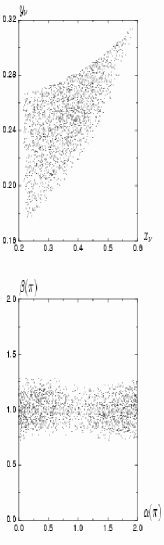
FIG. 1.: The parameter space of $(x_{\nu},y^{~{}}_{\nu})$ and $(\alpha,\beta)$ at the $3\sigma$ level.

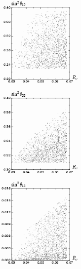
FIG. 2.: The outputs of $\sin^{2}\theta_{12}$, $\sin^{2}\theta_{23}$ and $\sin^{2}\theta_{13}$ versus $R_{\nu}$ at the $3\sigma$ level.

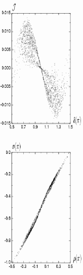
FIG. 3.: The outputs of $(\delta,{\cal J})$ and $(\rho,\sigma)$ at the $3\sigma$ level.

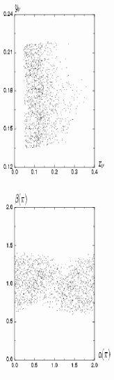
FIG. 4.: The parameter space of $(x_{\nu},y^{~{}}_{\nu})$ and $(\alpha,\beta)$ at the $2\sigma$ level in the seesaw case.

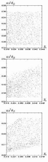
FIG. 5.: The outputs of $\sin^{2}\theta_{12}$, $\sin^{2}\theta_{23}$ and $\sin^{2}\theta_{13}$ versus $R_{\nu}$ at the $2\sigma$ level in the seesaw case.

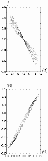
FIG. 6.: The outputs of $(\delta,{\cal J})$ and $(\rho,\sigma)$ at the $2\sigma$ level in the seesaw case.

REFERENCES

[1] SNO Collaboration, Q.R. Ahmad et al.,
Phys. Rev. Lett. 87 (2001) 071301; 89 (2002) 011301;
89 (2002) 011302.
[2] Super-Kamiokande Collaboration,
Y. Fukuda et al., Phys. Lett. B 467 (1999) 185;
S. Fukuda et al., Phys. Rev. Lett. 85 (2000) 3999;
Phys. Rev. Lett. 86 (2001) 5651;
Phys. Rev. Lett. 86 (2001) 5656.
[3] KamLAND Collaboration, K. Eguchi et al.,
Phys. Rev. Lett. 90 (2003) 021802.
[4] K2K Collaboration, M.H. Ahn et al.,
Phys. Rev. Lett. 90 (2003) 041801.
[5] See, e.g.,
J.N. Bahcall and C. Pea-Garay,
JHEP 0311 (2003) 004;
M.C. Gonzalez-Garcia and C. Pea-Garay,
Phys. Rev. D 68 (2003) 093003;
M. Maltoni, T. Schwetz, M.A. Trtola,
and J.W.F. Valle, hep-ph/0309130;
P.V. de Holanda and A.Yu. Smirnov, hep-ph/0309299; and references therein.
[6] For recent reviews with extensive references, see:
H. Fritzsch and Z.Z. Xing, Prog. Part. Nucl. Phys. 45 (2000) 1;
G. Altarelli and F. Feruglio, hep-ph/0206077, to appear in
Neutrino Mass - Springer Tracts in Modern Physics, edited by
G. Altarelli and K. Winter (2002);
S.F. King, hep-ph/0310204.
[7] H. Fritzsch, Phys. Lett. B 73 (1978) 317;
Nucl. Phys. B 155 (1979) 189.
[8] Z.Z. Xing, Phys. Lett. B 550 (2002) 178.
[9] M. Fukugita, M. Tanimoto, and T. Yanagida,
Phys. Lett. B 562 (2003) 273;
Prog. Theor. Phys. 89 (1993) 263.
[10] To be specific, we make use of the and
intervals of two neutrino mass-squared differences and three
lepton flavor mixing angles given by M. Maltoni et al in
Ref. [5].
[11] CHOOZ Collaboration, M. Apollonio et al.,
Phys. Lett. B 420 (1998) 397;
Palo Verde Collaboration, F. Boehm et al.,
Phys. Rev. Lett. 84 (2000) 3764.
[12] Particle Data Group, K. Hagiwara et al.,
Phys. Rev. D 66 (2002) 010001.
[13] Z.Z. Xing, Int. J. Mod. Phys. A 19 (2004) 1.
[14] C. Jarlskog, Phys. Rev. Lett. 55 (1985) 1039.
[15] T. Yanagida, in Proceedings of the Workshop on
Unified Theory and the Baryon Number of the Universe, edited by
O. Sawada and A. Sugamoto (KEK, Tsukuba, 1979), p. 95;
M. Gell-Mann, P. Ramond, and R. Slansky, in Supergravity,
edited by F. van Nieuwenhuizen and D. Freedman (North Holland,
Amsterdam, 1979), p. 315;
S.L. Glashow, in Quarks and Leptons, edited by
M. L et al. (Plenum, New York, 1980), p. 707;
R.N. Mohapatra and G. Senjanovic, Phys. Rev. Lett. 44, 912 (1980).
[16] K. Anderson et al., hep-ex/0402041.
[17] Z.Z. Xing and H. Zhang, Phys. Lett. B 569 (2003) 30.
[18] Z.Z. Xing, Phys. Rev. D 68 (2003) 073008.