Phenomenology of Twisted Moduli in Type I String Inspired Models

Abstract:

We make a first study of the phenomenological implications of twisted moduli in type I intersecting D5-brane models, focussing on the resulting predictions at the LHC using SOFTSUSY to estimate the Higgs and sparticle spectra. Twisted moduli can play an important role in giving a viable string realisation of sequestering in the limit where supersymmetry breaking comes entirely from the twisted moduli. We focus on a particular string inspired version of gaugino mediation in which the first two families are localised at the intersection between D5-branes, whereas the third family and Higgs doublets are allowed to move within the world-volume of one of the branes. The soft supersymmetry breaking third family sfermion mass terms are then in general non-degenerate with the first two families. We place constraints upon parameter space and predictions of flavour changing neutral current effects. Twisted moduli domination is studied and, as well as solving the most serious part of the SUSY flavour problem, is shown to be highly constrained. The constraints are weakened by switching on gravity-mediated contributions from the dilaton and untwisted T-moduli sectors. In the twisted moduli domination limit we predict a stop-heavy MSSM spectrum and quasi-degenerate lightest neutralino and chargino states with wino-dominated mass eigenstates.

1 Introduction

Superstrings provide a consistent way of unifying the four fundamental forces of Nature together within a single calculable theory. Until recently the weakly-coupled heterotic string theories were believed to offer the most promising framework in which to recover the observable low-energy Standard Model physics. However there was a major paradigm shift following the discovery of string dualities [1] that identified the separate string theories as different perturbative limits of an underlying 11d M-theory [2]. In particular the type I theory was recognised as a viable alternative to heterotic models, but with novel features such as a variable fundamental string scale $M_{\ast}$ and the presence of solitonic Dirichlet branes (D-branes) in the low-energy spectrum [3]. The flexibility of the string scale allows for models with large extra-dimensions [4] which open up the possibility of observing “stringy” experimental signatures at future colliders, and also non-standard gauge coupling unification at scales well below $M_{X}\sim 2\times 10^{16}$ GeV [5]. The Dirichlet branes are required for consistency, but provide a mechanism for localising matter and gauge fields (open string states) on a lower-dimensional slice of the full 10d spacetime in which gravity (closed strings) lives. These exciting new features have lead to a renaissance in string phenomenology, and renewed attempts to derive the (supersymmetric) Standard Model directly from a string theory compactification.

Recent developments have also motivated the study of higher-dimensional field theories that may describe the low-energy limit of string theory. Many string-inspired ideas and techniques including branes, orbifolding and Kaluza-Klein towers are now commonly used in model-building [6]. These models are studied with effective field theory (EFT) techniques valid up to some ultraviolet (UV) cutoff scale $\Lambda_{UV}<M_{\ast}$, where the string-like features cannot be resolved. In particular, branes can be associated with orbifold fixed points rather than the string-theoretic picture of hypersurfaces where open strings end, and strings are treated as point-particles. Also Standard Model states can be allocated arbitrarily to different points/branes in the higher-dimensional space, and often orbifold symmetry assignments dictate whether a particular coupling is allowed or not [7].

Many new models have been constructed to investigate quasi-realistic extensions of the (supersymmetric) Standard Model, where the extra-dimensional framework offers novel solutions to problems in cosmology, grand unification and flavour physics. In particular supersymmetry (SUSY) breaking has received a lot of attention in the context of higher-dimensional parallel-brane models. In these models a pair of parallel 4d branes are localised at either end of a 5d (or higher) bulk spacetime as shown in Figure 1. The Standard Model fields are localised on one brane while SUSY is broken at a distance on the other. These models are inspired by the strongly-coupled heterotic limit of 11d M-theory [8], and offer an attractive realisation of hidden-sector SUSY breaking. In the original hidden-sector models, the visible and SUSY breaking sectors occupied the same 4d spacetime, but direct communication between sectors was suppressed by inverse Planck-scale couplings. In contrast, the new parallel-brane models avoid direct couplings by delocalising – or “sequestering” – the two sectors at different points within the higher-dimensional space. Thus communication of SUSY breaking requires additional intermediary fields living in the bulk that couple to both sectors, and anomaly (gravity) [9] and gaugino [10] mediation are two recent examples. The combined Kähler potential that describes the visible, hidden and bulk sectors is assumed to have a particular sequestered form which is reminiscent of no-scale gravity models [11].

SUSY breaking masses and trilinears for Standard Model fields on the visible brane arise from higher-dimensional loops of particles living in the 5d bulk, since the contributions from direct couplings between sectors are found to be exponentially-suppressed by the separation $r$ and cutoff scale $\Lambda_{UV}$. The absence of significant direct couplings leads to an automatic suppression of flavour changing neutral currents (FCNCs) which alleviates the SUSY flavour problem since small off-diagonal squark/slepton mass-matrix elements are only reintroduced at the weak-scale through renormalisation group equation (RGE) running effects down from $\Lambda_{UV}$. However in the simplest models the viable regions of parameter space are very constrained. Also the special form of Kähler potential that leads to sequestering has been criticised as unlikely in explicit string constructions [12] and therefore the sequestered parallel-brane models are believed to be unrealistic.

Our goal in this work is to tackle these problems by embedding sequestering in a type I string model of the Minimal Supersymmetric Standard Model (MSSM) involving intersecting Dirichlet branes that may avoid the problems identified in Ref. [12]. We realise the sequestering mechanism by identifying the hidden sector with localised closed string twisted moduli states $Y_{k}$ [13, 14] that acquire SUSY breaking F-term vacuum expectation values (VEVs). These twisted moduli states can be spatially-separated away from (visible sector) MSSM fields that are trapped at the intersection between different D-branes with apparently no direct coupling to the twisted moduli. There are additional gravity mediation contributions to SUSY breaking from delocalised closed string states (dilaton and untwisted T-moduli) that freely move in the full 10d spacetime. In order to model the sequestering effect, we have previously proposed a modified Kähler potential for open string states that stretch between two different D5-branes and are localised away from the SUSY breaking twisted moduli fields [14]. In the absence of a complete theory of SUSY breaking we parameterise the F-terms using Goldstino angles [15]-[17] which control the relative contributions to the overall SUSY breaking, and we derive explicit expressions for the soft Lagrangian parameters [18].

We will consider an intersecting D5-brane model of the R-parity conserving MSSM [19, 20] where the first two MSSM families are trapped at the intersection between D-branes and the third family can couple directly to the twisted moduli. We consider the “single-brane dominance” limit with the MSSM gauge groups dominated by their components on the D$5_{2}$-brane, and use SOFTSUSY [21] to perform the RGE analysis below the grand unification scale of $M_{X}\sim 2\times 10^{16}$ GeV. We will focus our study around the twisted moduli domination limit where the only source of SUSY breaking originates from the localised twisted moduli fields, and this limit corresponds to sequestered models like gaugino mediated SUSY breaking ($\tilde{g}$MSB ) [10]. However we will also study the effect of including gravity mediation by smoothly varying the Goldstino angles, and we observe that the highly-constrained sequestered models are much less constrained after the inclusion of additional gravity mediated effects. The most severe FCNC constraints involving the first two families are satisfied within our model in two different ways. In the limit of twisted moduli domination the first and second family soft sfermion masses are negligible at the high-scale, and are only generated at low-energies by flavour-blind RGE effects. The inclusion of gravity mediation spoils this mechanism for suppressing FCNCs since soft sfermion masses are no longer negligible at the high-scale. Instead the SUSY flavour problem is ameliorated with the combination of heavy gluinos and the assumption of family-diagonal soft scalar mass matrices.

There have been many previous phenomenological analyses of type I D-brane constructions that use two Goldstino angles $\theta$, $\phi$ to parameterise the relative contributions to SUSY breaking from the dilaton, twisted and untwisted moduli F-term VEVs. However we present the first analysis to focus on the twisted moduli domination limit by proposing a Kähler potential to model the sequestering mechanism. Unlike previous studies with only D9-branes [22, 23], we consider a model involving intersecting D5-branes that enable open string MSSM states to be trapped at sub-manifolds of the full 10d spacetime that can be spatially-separated away from the localised twisted moduli source of SUSY breaking. Although twisted moduli arise in D9-brane constructions, it is impossible to sequester open string states away from the SUSY breaking since the open strings are free to move throughout the full D9-brane world-volume. Therefore we would not expect any sequestering to occur as these open strings can couple directly to the twisted moduli, and the standard Kähler potentials of Ref. [17] are valid.

The layout of the remainder of the paper is as follows. In section 2 we review our string-inspired gaugino mediation model of sequestering with twisted moduli. We also list the SUSY breaking soft parameters and motivate our choice of model parameters. Our results are presented in section 3 for the twisted moduli domination limit, and also more general cases involving the dilaton and untwisted T-moduli contributions. We also discuss constraints on our model from flavour changing processes and highlight some “benchmark” points with sample spectra. Our conclusions and discussion are given in section 4. For completeness we derive the SUSY breaking F-terms using Goldstino angles in Appendix A, and discuss the phenomenological problems facing a similar model with three degenerate families of intersection states in Appendix B.

2 Sequestering with twisted moduli

In this section we will review the results from our earlier paper [14] where we considered the contribution to SUSY breaking soft parameters from the F-term VEV of localised twisted moduli fields $Y_{k}$. Motivated by $\tilde{g}$MSB and non-perturbative instanton effects we proposed a modified Kähler potential for intersection states $C^{5_{1}5_{2}}$ that offers a string realisation of sequestering. Our framework allows us to study sequestering in the presence of other F-term VEVs from the dilaton and untwisted moduli fields - in this way we can study the interplay between $\tilde{g}$MSB ($F_{Y_{k}}\neq 0$) and pure gravity mediation ($F_{S},F_{T_{i}}\neq 0$) contributions. We will see that the strong constraints applying to sequestered models are relaxed through the addition of gravity mediation effects.

Our starting point is the low-energy effective supergravity (SUGRA) description of type I models compactified on toroidal orbifolds (or type IIB orientifolds) [17] which involve two stacks of perpendicular intersecting D5-branes at the origin fixed point as shown in Figure 1.

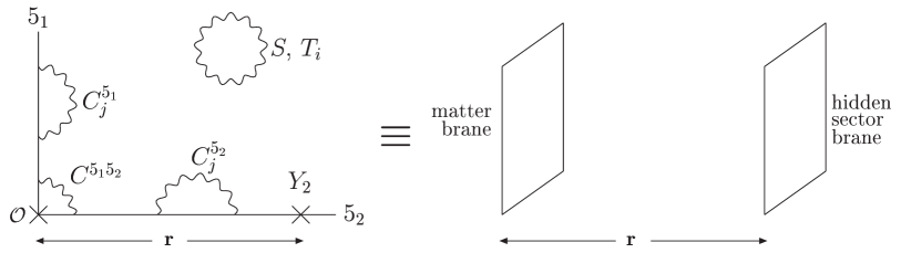
Figure 1: (left) A generic type I construction involving (perpendicular) intersecting D5-branes that share a common 4D overlap at the origin fixed point $\cal O$, where each D-brane carries a corresponding gauge group. The open and closed string states are shown, including twisted moduli that are trapped at orbifold fixed points marked by crosses. We propose that higher-dimensional field theory models (right) involving branes/fixed points are analogous to our string theory setup, where the matter (hidden sector) branes are equivalent to open strings at the origin $C^{5_{1}5_{2}}$ (twisted moduli) respectively.

Each stack of $N$ coincident D-branes supports a $U(N)$ super Yang-Mills gauge group where gauge fields arise as open strings with both ends attached to the same stack and carrying adjoint quantum numbers . Chiral matter fields are open strings carrying (bi)fundamental charges, with either (i) both ends attached to the same brane , e.g. $C^{5_{1}}_{j}$ and $C^{5_{2}}_{j}$; or alternatively (ii) open strings stretched between different D5-branes, e.g. $C^{5_{1}5_{2}}$ states. The string tension effectively localises the intersection states $C^{5_{1}5_{2}}$ at the common 4d overlap region $\cal O$, which is in contrast to the other open string states $C^{5_{1}}_{j}$ and $C^{5_{2}}_{j}$ that can freely move within the full 6d world-volume of their corresponding D5-brane. In addition to the open strings, there are also closed string states including three untwisted T-moduli $T_{i}$ (that parametrise the size of the extra-dimensional geometry since $(T_{i}+\overline{T}_{i})\sim R_{5_{i}}^{2}$) and the dilaton $S$ that are not confined to the world-volume of D-branes, but live in the full 10d space . However closed strings can also be localised in lower-dimensional sub-manifolds through the action of orbifolding, and twisted moduli states $Y_{k}$ are closed strings trapped around orbifold fixed points. In this work we will assume that SUSY breaking originates only from the closed string sector, i.e. when the auxiliary F-terms of the chiral superfields containing the moduli and dilaton acquire non-zero VEVs, i.e. $F_{S}$, $F_{T_{i}}$ and/or $F_{Y_{k}}\neq 0$.

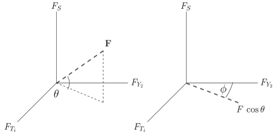
Figure 2: The relative contributions to the total SUSY breaking F-term ${\mathbf{F}}$ from each closed string F-term VEV ($F_{S}\,,\,F_{T_{i}}\,,\,F_{Y_{2}}$) can be parameterised by two Goldstino angles $(\theta\,,\,\phi)$ [15]-[17].

In the absence of a complete theory of SUSY breaking, such as gaugino condensation [25, 26], we represent the different F-term VEVs as components of an overall F-term vector ${\mathbf{F}}$ as shown in Figure 2. Varying the two Goldstino angles ($\theta,\,\phi$) allows us to control the relative contributions to SUSY breaking from each closed string sector .

$${\mathbf{F}}=\left(\begin{array}[]{c}F_{S}\\ F_{T_{i}}\\ F_{Y_{k}}\end{array}\right)\sim\left(\begin{array}[]{c}F\,\sin\theta\\ F\,\cos\theta\,\sin\phi\,\Theta_{i}\\ F\,\cos\theta\,\cos\phi\,\chi_{k}\end{array}\right)$$ (7)

where $F$ is the absolute magnitude of the total F-term ${\mathbf{F}}$. In this work we will only consider a single twisted moduli $Y_{2}$ and set $\chi_{2}=1$, $\chi_{k\neq 2}=0$ and we choose $\Theta_{i}=1/\sqrt{3}$ for simplicity.

The D-brane construction in the left panel of Figure 1 shows that it is possible to localise matter fields (open strings $C^{5_{1}5_{2}}$) and SUSY breaking fields (twisted moduli $Y_{2}$) at different fixed points in the compactified space . In the limit that the only non-zero F-term VEV arises from the localised twisted moduli $Y_{2}$, the setup was observed [13, 20] to be similar to the recent higher-dimensional field theory orbifold models of sequestering (right panel of Figure 1). In these orbifold models, matter fields and SUSY breaking can be arbitrarily localised at different fixed points/branes with apparently no direct coupling between the different sectors [9, 10]. Supersymmetry breaking can be communicated to the sequestered matter fields through the super-conformal anomaly [9] or transmission of bulk gauginos [10] at the 1-loop level, whereas the non-renormalisable higher-dimensional operators that give direct couplings are exponentially-suppressed after integrating out physics above the cutoff scale $\Lambda_{UV}$.

Following the ideas of Refs [13, 20], we propose that twisted moduli offer a mechanism for realising sequestering in type I D-brane constructions  between localised SUSY breaking fields ($Y_{2}$) and spatially-separated matter fields ($C^{5_{1}5_{2}}$ and $C^{5_{1}}_{j}$). However our D-brane framework also allows for some open strings states ($C^{5_{2}}_{j}$) to couple directly to the twisted moduli F-term VEV, and this can be exploited to generate a hierarchy between the soft scalar masses of different states at the high-scale. In the next section we will outline a string-inspired MSSM model where the third family and Higgs doublets are identified with $C^{5_{2}}_{j}$ states and consequently have hierarchically larger soft masses (at the high-scale) compared to the first two MSSM generations which are sequestered at the origin as $C^{5_{1}5_{2}}$ states. We will study the phenomenology of this model as we move away smoothly from the twisted moduli dominated limit ($\cos\theta=\cos\phi=1$) and introduce contributions to the SUSY breaking from the dilaton and T-moduli F-terms. Unlike previous analyses [22, 23], we will focus on the twisted moduli domination limit. We will show that the strong constraints applying to that limit are relaxed through the addition of gravity mediation effects.

2.1 String-Inspired Gaugino Mediation (SI$\tilde{g}$M)

In this section we will outline our model of sequestering as shown in Figure 3. We choose to study this particular setup because it is the closest string-inspired model to gaugino mediation in the literature. It is important to emphasise that a model where all three MSSM families, rather than just the first two, are intersection states is not directly motivated by string constructions, moreover if such a model is enforced by hand it leads to phenomenological problems as discussed in Appendix B.

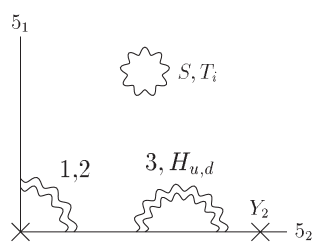
Figure 3: The allocation of open and closed string states in a string-inspired MSSM model. The first/second family ($1,2$) are intersection states $C^{5_{1}5_{2}}$, while the third family ($3$) and Higgs doublets ($H_{u},H_{d}$) are $C^{5_{2}}_{j}$ states. The twisted moduli $Y_{2}$ is trapped at a fixed-point within the D$5_{2}$-brane, whereas the dilaton $S$ and untwisted moduli $T_{i}$ live in the full 10d spacetime.

The model studied here suppresses the most dangerous FCNCs involving the first and second families using two different mechanisms. Firstly in the limit of twisted moduli domination, the first/second family scalar masses are negligible at the high-scale due to sequestering. This leads to universal low-energy squark and slepton mass matrices that are approximately diagonal due to flavour-blind RGE running effects in analogy to $\tilde{g}$MSB models. Moving away from the twisted moduli limit by introducing gravity mediation contributions removes the sequestering, and so the first/second family soft scalar masses are no longer negligible at the high scale which spoils this mechanism for suppressing FCNCs. However, we find that the physical gluino and squark sparticle masses are sufficiently heavy to ameliorate the FCNC constraints when we make the additional assumption that the soft scalar mass matrices are diagonal in family-space at the high-scale. The weaker experimental constraints on the third family FCNCs allows us to treat these fields differently. Direct coupling to the twisted moduli gives heavier third family soft masses at the high-scale that prove helpful in achieving successful electroweak symmetry breaking (EWSB) and a sufficiently heavy lightest CP-even Higgs mass.

Our setup involves two stacks of perpendicular intersecting D5-branes where a copy of the MSSM gauge group $G_{MSSM}$ lives on both stacks. We assume a hierarchy between the different toroidal compactification radii $R_{5_{2}}\gg R_{5_{1}}$ which implies that the corresponding gauge couplings on each brane are also hierarchical with $g_{5_{2}}\ll g_{5_{1}}$. This assumption allows us to treat the $5_{1}$-brane (and any attached open string states) as effectively localised at the 4d intersection region between branes. Also the resulting hierarchy between gauge couplings ensures that the diagonal product of MSSM gauge groups is dominated by the components living within the $5_{2}$-brane. This “single brane dominance” limit allows for gauge coupling unification on the $5_{2}$-brane. However the $5_{1}$-brane could not be ignored from the start since it facilitates the localisation of open string states $C^{5_{1}5_{2}}$ at the 4d intersection which we identify with the first and second quark/lepton families. In contrast the third family and Higgs doublets are allocated to open string states $C^{5_{2}}_{j}$ with both ends attached to the $5_{2}$-brane . We choose the following allocation of MSSM superfields:

$$Q_{iL}\,,\,L_{iL}\,,\,U_{iR}^{c}\,,\,D_{iR}^{c}\,,\,E_{iR}^{c} \equiv C^{5_{1}5_{2}}\hskip 28.45274pt(i=1,2)$$ (8)

$$U_{3R}^{c}\,,\,D_{3R}^{c}\,,\,E_{3R}^{c}\equiv C^{5_{2}}_{3}\hskip 14.22636pt,\hskip 14.22636ptH_{u}\,,\,H_{d} \equiv C^{5_{2}}_{2}\hskip 14.22636pt,\hskip 14.22636ptQ_{3L}\,,\,L_{3L}\equiv C^{5_{2}}_{1}$$

At the renormalisable level, the superpotential is constrained by string selection rules [17] to have the following allowed terms (subject to gauge-invariance) :

$$W_{ren}\sim C^{5_{2}}_{1}\,C^{5_{2}}_{2}\,C^{5_{2}}_{3}+C^{5_{2}}_{3}\,C^{5_{1}5_{2}}\,C^{5_{1}5_{2}}$$ (9)

and the allocation of states in Eq.(8) leads to hierarchical Yukawa (and trilinear) matrices with a non-zero (33) entry, and the other (smaller) elements of the Yukawa matrices required to generate the other fermion masses are assumed to arise from higher-dimensional operators. We will also impose an R-parity (or gauge-invariance if the model is embedded within a larger gauge group) to forbid the R-parity violating string-allowed superpotential terms given by the second term in Eq.(9). Notice that the renormalisable superpotential contains no Higgsino mixing term $\mu H_{u}H_{d}$.

In a previous paper [14] we discovered that a straightforward application of low-energy supergravity formulae for soft parameters, using the standard type I Kähler potentials for open string states [17] and Goldstino parameterisation of SUSY breaking, does not lead to sequestered first/second family ($C^{5_{1}5_{2}}$) soft scalar masses in the limit of twisted moduli domination. In fact $m_{C^{5_{1}5_{2}}}^{2}$ is independent of the separation $r\sim{\cal O}(R_{5_{2}})$ between the SUSY breaking $Y_{2}$ and the D5-brane intersection. In Ref. [14] we proposed a modified Kähler potential $K_{C^{5_{1}5_{2}}}$ for $C^{5_{1}5_{2}}$ states with an explicit dependence on $r$ that, by construction, exhibits sequestering in the twisted moduli domination limit. Note that we have chosen a sequestering exponential factor $e^{-(M_{\ast}R_{5_{2}})^{2}}=e^{-(T_{2}+\overline{T_{2}})/4}$ which is different from the usual Yukawa-like factor in the parallel-brane sequestered models, since we assume that this suppression factor originates from a non-perturbative instanton effect due to strings stretching between different fixed points [27]. The relevant terms in the Kähler potential for the open string states in Eq.(8) are :

$$K_{C^{5_{2}}_{1}}=\frac{|C^{5_{2}}_{1}|^{2}}{T_{3}+\overline{T_{3}}}\hskip 28.45274pt,\hskip 28.45274ptK_{C^{5_{2}}_{2}}=\frac{\,|C^{5_{2}}_{2}|^{2}\,}{S+\overline{S}}\hskip 28.45274pt,\hskip 28.45274ptK_{C^{5_{2}}_{3}}=\frac{|C^{5_{2}}_{3}|^{2}}{T_{1}+\overline{T_{1}}}$$ (10)

$$K_{C^{5_{1}5_{2}}}=\frac{|C^{5_{1}5_{2}}|^{2}}{\sqrt{S+\overline{S}}\,\sqrt{T_{3}+\overline{T_{3}}}}\,exp\left[\frac{X^{2}}{6}\left(1-e^{-(T_{2}+\overline{T_{2}})/4}\right)\right]\hskip 42.67912pt$$ (11)

where we have assumed that all Kähler potentials are “canonical”, i.e. diagonal ; and the modified $C^{5_{1}5_{2}}$ potential involves the combination $X=Y_{2}+\overline{Y_{2}}-\delta_{GS}\,{\mathrm{l}n}(T_{2}+\overline{T_{2}})$ due to modular anomaly cancellation arguments [24]. In the limit of vanishing compactification radius $R_{5_{2}}=\sqrt{T_{2}+\overline{T_{2}}}/2\longrightarrow 0$, we recover the usual expression for $K_{C^{5_{1}5_{2}}}$  [17]. For the closed string dilaton and moduli states, we use the standard Kähler potentials:

$$K(S,\overline{S},T_{i},\overline{T_{i}},Y_{2},\overline{Y_{2}})=-\ln(S+\overline{S})-\sum_{i=1}^{3}\ln(T_{i}+\overline{T_{i}})+\hat{K}\left[Y_{2}+\overline{Y_{2}}-\delta_{GS}\,\ln(T_{2}+\overline{T_{2}})\right]\hskip 14.22636pt$$ (12)

but we choose to leave the precise form of the twisted moduli Kähler potential $\hat{K}$ as an unknown function with an argument $X=Y_{2}+\overline{Y_{2}}-\delta_{GS}\,{\mathrm{l}n}(T_{2}+\overline{T_{2}})$  [29]. We will choose to fix the first and second derivatives $\hat{K}^{\prime}\equiv\partial_{X}\hat{K}(X)=0$ and $\hat{K}^{\prime\prime}\equiv\partial_{X}^{2}\hat{K}(X)=1$ as discussed in section 2.1.2. However the mixing induced between $T_{2}$ and $Y_{2}$ by $\hat{K}(X)$ means that the Kähler metric is no longer diagonal (after ignoring negligible VEVs for the matter fields). Therefore, in order to invert the Kähler metric, we use the same techniques as Ref [22, 23] to define the SUSY breaking with Goldstino angles where $F_{T_{2}}$ and $F_{Y_{2}}$ are expanded in inverse powers of the $T_{2}+\overline{T_{2}}$ VEV as discussed in Appendix A.

2.1.1 SUSY breaking parameters

The soft Lagrangian ${\cal L}_{soft}$ is given by:

$$-{\cal L}_{soft}^{MSSM}=\frac{1}{2}\left(M_{1}\tilde{B}\tilde{B}+M_{2}\tilde{W}\tilde{W}+M_{3}\tilde{g}\tilde{g}\right)+h.c.\hskip 170.71652pt$$

$$+(A^{u}_{ij}\,Y^{u}_{ij})\,\tilde{u}^{\ast}_{iR}\tilde{Q}_{jL}H_{u}-(A^{d}_{ij}\,Y^{d}_{ij})\,\tilde{d}^{\ast}_{iR}\tilde{Q}_{jL}H_{d}-(A^{e}_{ij}\,Y^{e}_{ij})\,\tilde{e}^{\ast}_{iR}\tilde{L}_{jL}H_{d}+h.c.\hskip 42.67912pt$$ (13)

$$+\tilde{Q}_{iL}^{\dagger}\left(m_{\tilde{Q}}^{2}\right)_{ij}\tilde{Q}_{jL}+\tilde{L}_{iL}^{\dagger}\left(m_{\tilde{L}}^{2}\right)_{ij}\tilde{L}_{jL}+\tilde{u}_{iR}^{\ast}\left(m_{\tilde{u}}^{2}\right)_{ij}\tilde{u}_{jR}+\tilde{d}_{iR}^{\ast}\left(m_{\tilde{d}}^{2}\right)_{ij}\tilde{d}_{jR}$$

$$+\tilde{e}_{iR}^{\ast}\left(m_{\tilde{e}}^{2}\right)_{ij}\tilde{e}_{jR}+m_{H_{u}}^{2}H_{u}^{\ast}H_{u}+m_{H_{d}}^{2}H_{d}^{\ast}H_{d}-\left(B\mu H_{u}H_{d}+h.c.\right)$$

where ($\tilde{B},\tilde{W},\tilde{g}$) are the bino, wino and gluino gauginos respectively; ($H_{u},H_{d}$) are the scalar components of the two Higgs doublets; and $\tilde{u}_{iR},\tilde{d}_{iR},\tilde{e}_{iR}\left(\tilde{Q}_{iL},\tilde{L}_{iL}\right)$ are the squark/slepton singlets (doublets) respectively.

We apply standard SUGRA formulae to Eqs.(10-12) - using the SUSY breaking F-terms from Eq.(56) with $k=1$ - to obtain expressions for the squark/slepton mass-squared matrices $m^{2}$, the gaugino masses $M_{i}$, and the soft trilinear matrices $A_{ij}$ [18]. These soft parameters provide grand unified theory (GUT) scale boundary conditions for the RGE analysis. We do not specify $B$ or $\mu$ at the GUT-scale since they can be exchanged for $\tan\beta$ and the measured value of $M_{Z^{0}}$ by imposing radiative EWSB at the weak-scale.

$\bullet$ Soft scalar masses:

Using the canonically-normalised Kähler potentials in Eq.(10,11), we find that the squark and slepton mass-squared matrices take the following form in family space at the high-scale:

$$m_{\tilde{Q}}^{2}\,,\,m_{\tilde{L}}^{2}\,,\,m_{\tilde{u}}^{2}\,,\,m_{\tilde{d}}^{2}\,,\,m_{\tilde{e}}^{2}=\left(\begin{array}[]{ccc}m_{C^{5_{1}5_{2}}}^{2}&m_{C^{5_{1}5_{2}}}^{2}&0\\ m_{C^{5_{1}5_{2}}}^{2}&m_{C^{5_{1}5_{2}}}^{2}&0\\ 0&0&m_{C^{5_{2}}_{1,3}}^{2}\end{array}\right)$$ (17)

where the degenerate first/second family mass-squared is given by:

$$m_{C^{5_{1}5_{2}}}^{2}=m_{3/2}^{2}\left[1-\frac{3}{2}\sin^{2}\theta-\frac{1}{2}\cos^{2}\theta\,\sin^{2}\phi-\left(1-e^{-(T_{2}+\bar{T}_{2})/4}\right)\cos^{2}\theta\cos^{2}\phi\right.\hskip 42.67912pt$$ (18)

$$-\frac{X}{3}\,\cos^{2}\theta\sin^{2}\phi\,\delta_{GS}\left(1-e^{-(T_{2}+\bar{T}_{2})/4}\right)+\frac{X^{2}}{96}\cos^{2}\theta\sin^{2}\phi\,e^{-(T_{2}+\bar{T}_{2})/4}(T_{2}+\bar{T}_{2})^{2}\hskip 14.22636pt$$

$$-\left.\frac{1}{16\sqrt{3}}\cos^{2}\theta\cos\phi\sin\phi\,e^{-(T_{2}+\bar{T}_{2})/4}\left\{8(T_{2}+\bar{T}_{2})+\delta_{GS}\,X\right\}X\right]+{\cal O}\left[\frac{\delta_{GS}\,e^{-(T_{2}+\overline{T_{2}})/4}}{(T_{2}+\overline{T_{2}})}\right]$$

with $X=Y_{2}+\overline{Y_{2}}-\delta_{GS}\,{\mathrm{l}n}(T_{2}+\overline{T_{2}})$; and the third family mass-squared is

$$m_{C^{5_{2}}_{1}}^{2}\,,\,m_{C^{5_{2}}_{3}}^{2}=m_{3/2}^{2}\left(1-\cos^{2}\theta\,\sin^{2}\phi\right)$$ (19)

In the twisted moduli dominated limit, $m_{C^{5_{1}5_{2}}}^{2}\longrightarrow 0$ due to the exponential suppression. Only diagonal mass matrix entries are generated by gauge loops in the renormalisation to low energies. Departing from twisted moduli domination introduces a non-negligible $m_{C^{5_{1}5_{2}}}^{2}$, and then we require an additional family symmetry to suppress the $(1,2)$ entries at the GUT scale in order to avoid predicting large FCNCs. In practice then, for all numerical estimates, we will use family diagonal boundary conditions for sfermion soft masses.

The Higgs doublet soft scalar masses-squared are universal at the high-scale:

$$m_{H_{u}}^{2}\,,\,m_{H_{d}}^{2}\equiv m_{C^{5_{2}}_{2}}^{2}=m_{3/2}^{2}\left(1-3\sin^{2}\theta\right)$$ (20)

$\bullet$ Soft gaugino masses:

The soft gaugino masses explicitly depend on the gauge couplings. In this work we assume that all three Standard Model couplings unify to a common value at the usual GUT-scale $M_{GUT}\sim 2\times 10^{16}$ GeV, and the unified gauge coupling is determined by running the RGEs up from the weak-scale. The soft masses are given by:

$$M_{\alpha}=\frac{\sqrt{3}m_{3/2}\,g_{\alpha}^{2}}{8\pi}\cos\theta\left[\frac{\sin\phi}{\sqrt{3}}\left\{T_{2}+\bar{T_{2}}+\frac{s_{\alpha}}{4\pi}\delta_{GS}\right\}\right.\hskip 142.26378pt$$ (21)

$$-\left.\cos\phi\left\{\frac{\delta_{GS}}{T_{2}+\bar{T}_{2}}-\frac{s_{\alpha}}{4\pi}\right\}\right]+{\cal O}\left[\frac{\delta_{GS}}{(T_{2}+\overline{T_{2}})^{2}}\right]$$

where for simplicity we have chosen the $s_{\alpha}$ parameters to be the 1-loop beta-function coefficients (i.e. $s_{\alpha}=2\pi(33/5,1,-3)$ for $\alpha=U(1)_{Y}\,,\,SU(2)_{L},\,,\,SU(3)_{C}$) in agreement with Refs [22, 23]. This can happen in ${\mathcal{Z}}_{3}$ and ${\mathcal{Z}}_{7}$ orbifold models, but in general $s_{\alpha}$ are highly model dependent parameters related to the Green-Schwarz coefficients [24].

$\bullet$ Soft trilinears:

Recall that the allocation of MSSM states in Eq.(8) is constrained by the string selection rules in Eq.(9) to give a hierarchical Yukawa (and trilinear) texture with a dominant (33) entry at leading-order. The other elements are assumed to arise from (unspecified) higher-dimensional operators in order to match the measured first and second family fermion masses at the weak-scale after RGE running. Therefore we expect that (generically) the Yukawa matrices have non-diagonal elements even at the high-scale. However for simplicity we choose to impose GUT-scale boundary conditions on the trilinear couplings $A^{f}_{ij}\,Y^{f}_{ij}$ ($f=u,d,e$) in Eq.(13) that ignore the effect of any higher-dimensional operators. Then the GUT-scale trilinears have a single non-zero (33) element:

$$A^{f}_{ij}\,Y^{f}_{ij}=\left(\begin{array}[]{ccc}0&0&0\\ 0&0&0\\ 0&0&{\cal A}\,Y^{f}_{33}\end{array}\right)\hskip 28.45274pt(f=u,d,e)$$ (25)

where $Y^{f}_{33}$ is the (33) element of the (running) Yukawa matrix $Y^{f}$ at the GUT-scale. Notice that we are not explicitly imposing a hierarchical (33) texture on the GUT-scale Yukawa matrices, since their form at the GUT-scale is determined by running the RGEs up from the correct weak-scale values (after CKM mixing). The universal soft trilinear ${\cal A}$ is found to be:

$${\cal A}\equiv A_{C^{5_{2}}_{1}C^{5_{2}}_{2}C^{5_{2}}_{3}}=-m_{3/2}\cos\theta\,\sin\phi+{\cal O}\left[\frac{\delta_{GS}}{(T_{2}+\overline{T_{2}})^{2}}\right]$$ (26)

where we have assumed no explicit dilaton/moduli dependence in the Yukawa couplings .

2.1.2 Choice of model parameters

At this stage we have a variety of (arbitrary) independent parameters, and in order to make progress we make the theoretically-motivated assumptions given in Table 1 to leave four independent parameters $m_{3/2}$, $\tan\beta$, $\phi$ and $\theta$ to scan over. Note that the $\theta$ Goldstino angle is constrained to the range $0\leq\theta\leq\arcsin(1/\sqrt{3})$ to avoid tachyonic soft Higgs doublet masses at the GUT-scale as shown by Eq.(20). This constraint allows the electroweak symmetry to be radiatively broken by running the RGEs down to the weak-scale instead of a tree-level breaking at the GUT-scale.

Parameter	Constraint	Comments
${}^{\dagger}\,$ gravitino mass $m_{3/2}$	100 - 10,000   GeV	sets SUSY breaking scale
${}^{\dagger}\,$ Goldstino angle $\theta$	$0\leq\theta\leq\arcsin(1/\sqrt{3})$	for Higgs masses $m_{C^{5_{2}}_{2}}^{2}\geq 0$
${}^{\dagger}\,$ Goldstino angle $\phi$	$0\leq\phi\leq\pi/2$
Goldstino angles $\Theta_{1,2,3}$	$1/\sqrt{3}$
Kähler potential $\hat{K}(X)$	$\partial_{X}\hat{K}=0$,   $\partial_{X}^{2}\hat{K}=1$	vanishing F.I. term
Green-Schwarz coefficient $\delta_{GS}$	-10	agrees with [22, 23]
VEV of ($T_{2}+\bar{T}_{2}$)	50	from gauge unification
VEV of ($Y_{2}+\bar{Y}_{2}$)	0	from gauge unification
${}^{\dagger}\,$ tan$\beta$	2-50
$M_{GUT}$		determined by RGE running
Sign of $\mu$-parameter	$sgn(\mu)>0$	motivated by $b\rightarrow s\,\gamma$, $g_{\mu}-2$

Table 1: The choice of high-scale (upper) and low-scale (lower) parameters for our model, where those marked with $\dagger$ are input parameters.

In section 2.1 we commented that the twisted moduli Kähler potential is an unknown function of $Y_{2},T_{2}$ and $\delta_{GS}$ with an argument $X=Y_{2}+\overline{Y_{2}}-\delta_{GS}\,{\mathrm{l}n}(T_{2}+\overline{T_{2}})$ required to cancel modular anomalies [24]. We have chosen to follow previous analyses [22, 23] and assume that the derivatives of $\hat{K}(X)$ satisfy the following constraints: $\hat{K}^{\prime}\equiv\partial_{X}\hat{K}(X)=0$ and $\hat{K}^{\prime\prime}\equiv\partial_{X}^{2}\hat{K}(X)=1$, where $\partial_{X}\hat{K}=0$ ensures that potentially problematic Fayet-Illiopoulos terms $\xi_{FI}\sim\hat{K}^{\prime}$ vanish. The Green-Schwarz parameter is a model-dependent negative integer ${\cal O}(-10)$, and for simplicity we set $\delta_{GS}=-10$.

In Appendix A we discuss how to diagonalise the Kähler metric when it is non-diagonal due to the mixing between $T_{2}$ and $Y_{2}$ induced by $\hat{K}(X)$. We can define the SUSY breaking F-terms, and therefore the soft parameters, by expanding in inverse-powers of the $T_{2}+\overline{T_{2}}$ VEV. This expansion is reliable when $T_{2}+\overline{T_{2}}$ is sufficiently large in string-scale $M_{\ast}$ units. We also know that the (tree-level) gauge couplings $g_{\alpha}$ are functions of $T_{2}+\overline{T_{2}}$ and $Y_{2}+\overline{Y_{2}}$ through the gauge kinetic functions $f_{\alpha}=T_{2}+\frac{s_{\alpha}}{4\pi}Y_{2}$ and the relation ${\mathrm{R}e}f_{\alpha}=4\pi/g_{\alpha}^{2}$. However the parameters $s_{\alpha}$ are not equal for all three groups of the MSSM, which implies that at tree-level the gauge couplings do not unify to a single coupling $g_{GUT}^{2}\approx 4\pi/25$. Thus in order to achieve unification we must appeal to (unspecified) higher-order corrections to the gauge kinetic functions. In this work we will assume that these higher-order corrections only account for a small correction to the tree-level value and so we choose that:

$$(T_{2}+\overline{T_{2}})=50\hskip 28.45274pt{\mathrm{a}nd}\hskip 28.45274pt(Y_{2}+\overline{Y_{2}})=0$$ (27)

which is entirely consistent with coupling unification and different $s_{\alpha}$. This value of $T_{2}+\overline{T_{2}}$ is also sufficiently large to justify the series expansion of F-terms, and we can neglect the higher-order corrections to the soft parameters in Eqs.(18,21,26).

Throughout our analysis we will neglect CP-phases and consequently keep all soft scalar squared-masses positive-definite. We demand a neutral lightest supersymmetric particle (LSP), and also that the low-energy gluino mass is not much larger than 1-2 TeV from fine-tuning arguments [32]. In section 3.5 we will compare generalised bounds on mass-insertion deltas derived from CP-conserving FCNC experimental data [33] to check that our model is allowed. We will take the Higgsino $\mu$-parameter to be positive which is consistent with the $b\longrightarrow s\gamma$ observations and recent favoured values of $g_{\mu}-2$.

Sparticle	Lower bound (GeV)	Sparticle	Lower bound (GeV)
lightest Higgs   $H_{1}^{0}$	111.4	sleptons $\tilde{e},\tilde{\mu}$	88
neutralino $\chi_{1}^{0}$	37	stop $\tilde{t}_{1}$	86.4
chargino $\chi_{1}^{\pm}$	67.7	sbottom $\tilde{b}_{1}$	91
gluino $\tilde{g}$	195	squarks $\tilde{u},\tilde{d},\tilde{c},\tilde{s}$	250
stau $\tilde{\tau}_{1}$	76	sneutrino $\tilde{\nu}_{1}$	43.1

Table 2: Experimental lower bounds on sparticle masses from direct searches [34]. The first column of experimental limits provide the strongest constraints, where the MSSM-like lightest Higgs mass includes a 3 GeV theoretical uncertainty.

In addition to these theoretical constraints, we use the experimental limits on sparticle masses given in Table 2 to constrain our allowed parameter space. Note that the experimental limit for the MSSM-like lightest Higgs $h^{0}$ is $m_{h^{0}}=114.4$ GeV. We use $111.4$ GeV, since we include a $\pm 3$ GeV error on SOFTSUSY’s prediction of $m_{h^{0}}=114.4$ GeV. We will comment on the sparticle(s) that provide the strongest constraint to the viable parameter space for a variety of model points.

We use the default version of SOFTSUSY 1.7.2 [21], which uses 2-loop RGEs for all parameters except sfermion masses and soft trilinears. Pole values for sparticle masses are calculated with one (and in sensitive cases) two-loop threshold contributions. We refer the reader to the SOFTSUSY manual [21] for more details. Electroweak gauge unification fixes the scale $M_{X}$ at which the boundary conditions on SUSY breaking masses are fixed:

$$g_{1}(M_{X})=g_{2}(M_{X})$$ (28)

For $g_{3}$, we assume unknown high-scale corrections bring the prediction $g_{3}(M_{X})=g_{1}(M_{X})$ into line with the input value of the Standard Model $\alpha_{s}(M_{Z})^{\overline{M}S}=0.1172$, which is used for our analysis. We also use $m_{t}=174.3$ GeV, $m_{b}(m_{b})^{\overline{M}S}=4.25$ GeV, the SOFTSUSY defaults.

For the analysis of flavour changing neutral currents, a detailed Yukawa texture is considered beyond the scope of the present paper. We therefore allow low energy data on fermion masses and mixings to set the electroweak-scale Yukawa couplings (with an additional assumption about whether quark mixing resides entirely in the down, or up quark sector). We neglect neutrino masses and mixings, which will have an unimportant effect on the rest of the sparticle spectrum. We have added the boundary conditions in Eqs.(17-26) to the SOFTSUSY code.

In our analysis we consider also a slightly modified model from Eq.(8) in which the superfields $D^{c}_{3R},E^{c}_{3R}$ are reassigned to $C_{1}^{5_{2}}$. String selection rules will then forbid a renormalisable bottom and tau Yukawa coupling, allowing low $\tan\beta$ without changing the results for the soft masses according to Eq.(19).

3 Results

In this section we will study the phenomenology of different SI$\tilde{g}$M model points around the twisted moduli domination limit ($\theta=\phi=0$). We observe that the viable parameter space is greatly increased by including contributions to the SUSY breaking from gravity mediation ($F_{S}$ and/or $F_{T_{i}}\neq 0$) by increasing $\theta$, $\phi$. In contrast we will consider the heavily constrained untwisted T-moduli domination limit ($\theta=0$, $\phi=\pi/2$) and study the effect of including twisted moduli by reducing $\phi$. We also study a couple of intermediate points with both $\theta$ and $\phi$ non-zero, and perform some scans over $\theta$–$\phi$ with fixed $m_{3/2}$ and $\tan\beta$. We will discuss the implications of FCNC bounds on our models, and give sample sparticle spectra for some “benchmark” points.

3.1 Twisted moduli domination: $\theta=\phi=0$

We begin our phenomenological analysis with the twisted moduli domination limit which has not been previously studied in the literature. In this limit the first and second family soft scalar masses are exponentially small in comparison to the third family and Higgs soft masses, and the dominant soft trilinear vanishes as shown in the first column of Table 3. As a result the viable parameter space is restricted to a very narrow range of $\tan\beta$ values, although there is still significant variation in the allowed physical masses of the (a) lightest Higgs, (b) gluino, (c) neutralino and (d) first/second family squarks as shown in Figure 4. The different treatment of the three families is highlighted in Figure 5 where the first/second family squarks are significantly lighter than the lightest stop states as a result of the hierarchy of soft masses at the GUT-scale. This leads to a characteristic sparticle spectrum which we have labelled “stop-heavy MSSM” [20]. This constrasts with the usual minimal SUGRA case where one stop is lighter than the other squarks due to top-Yukawa RGE and mixing effects.

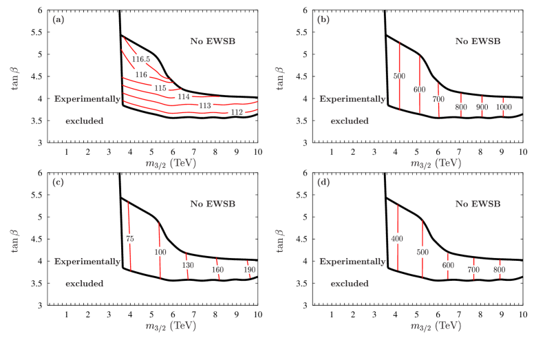
Figure 4: Maps of viable parameter space and mass contours of (a) lightest Higgs $h^{0}$, (b) gluino $\tilde{g}$, (c) neutralino $\chi_{1}^{0}$ and (d) lightest squark $\tilde{q}=\tilde{u},\tilde{d},\tilde{c},\tilde{s}$ for $\theta=\phi=0$.

Soft mass/trilinear	(a) $\phi=0$	(b) $\phi=0.05$	(c) $\phi=0.07$	(d) $\phi=0.1$
(in $m_{3/2}$ units)
1st/2nd family $C^{5_{1}5_{2}}$	0.002	0.572	0.801	0.143
3rd family $C^{5_{2}}_{1,3}$	1	0.999	0.998	0.995
Higgses $C^{5_{2}}_{2}$	1	1	1	1
Trilinear $A_{C^{5_{2}}_{1}C^{5_{2}}_{2}C^{5_{2}}_{3}}$	0	-0.050	-0.070	-0.100
$M_{1}$	0.121	0.138	0.145	0.155
$M_{2}$	0.024	0.069	0.087	0.114
$M_{3}$	-0.045	0.020	0.046	0.085

Table 3: Numerical values of soft SUSY breaking parameters (in units of $m_{3/2}$) as $\phi$ is increased with $\theta=0$ kept fixed. We assume that the unified GUT-scale gauge coupling is $\alpha_{GUT}\approx 1/25$ in order to estimate the relative size of the gaugino masses.

Low values of $m_{3/2}\leq 3.5$ TeV are forbidden by the chargino $\chi_{1}^{\pm}$ experimental bound, whereas the Higgs bound $m_{h^{0}}>111$ GeV rules out very small values of $\tan\beta\stackrel{{\scriptstyle<}}{{{}_{\sim}}}4$. The other constraint comes from the requirement of valid radiative EWSB which rules out the space for $\tan\beta>4.5$ and $m_{3/2}>3.5$ TeV.

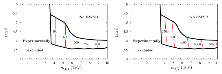
Figure 5: Comparison of the mass contours for (left) first/second family squarks $\tilde{q}=\tilde{u},\tilde{d},\tilde{c},\tilde{s}$ and (right) stop squark $\tilde{t}_{1}$ for $\theta=\phi=0$.

There is an intriguing experimental signature of the twisted moduli limit from the quasi-degeneracy of the lightest neutralino and chargino states. This is similar to the situation in anomaly mediated SUSY breaking [9], and can be understood from the first column of Table 3 since the soft bino and wino gaugino masses have the ratio $M_{1}\approx 5\,M_{2}$. Therefore the lightest chargino mass eigenstate ($m_{\chi_{1}^{\pm}}$) is roughly the wino ($M_{2}$), and so is the lightest neutralino mass eigenstate ($m_{\chi_{1}^{0}}$) (up to electroweak corrections). The light Higgs mass $m_{h^{0}}<117$ GeV and heavy stop are other indicators of the scenario.

3.2 Moving away from twisted moduli domination by switching on T-moduli

In this section we will try to understand the effect of the twisted moduli F-term on the viable parameter space by increasing the value of $\phi$ to move away from the twisted moduli domination limit. We keep $\theta=0$ fixed which eliminates any contributions from the dilaton ($F_{S}=0$), and so increasing $\phi$ includes the untwisted T-moduli F-term contributions to the overall SUSY breaking VEV.

In Table 3 we show how the numerical values of the GUT-scale soft parameters (in $m_{3/2}$ units) are affected by increasing $\phi$. The common first and second family soft scalar masses rapidly increase, while the third family and Higgses remain more or less constant. The soft trilinear is no longer vanishing, and the soft gaugino masses also rise - in fact the gluino soft mass changes sign relative to the twisted moduli domination limit.

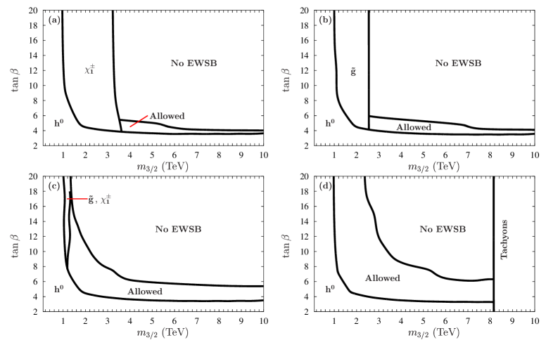
Figure 6: The viable parameter space (Allowed) opens up as $\phi$ is increased with $\theta=0$ fixed; (a) $\phi=0$, (b) $\phi=0.05$, (c) $\phi=0.07$ and (d) $\phi=0.1$. Note that (d) extends up to include $\tan\beta=50$. We label the surrounding regions of parameter space by the sparticle(s) that provide the strongest constraints.

We plot the evolution of the viable parameter space in Figure 6, and as expected we observe that the space rapidly opens up with increasing $\phi$. In each case the lightest Higgs mass experimental limit excludes very small $\tan\beta$ regions. Moving from (a) to (d) we see that the strongest constraints on the lower $m_{3/2}$ region of parameter space comes from the chargino, gluino and finally lightest Higgs experimental bounds. The remaining forbidden space is ruled out by the requirement of EWSB. It is interesting to observe that for larger values of $\phi\stackrel{{\scriptstyle>}}{{{}_{\sim}}}0.1$ the large-$m_{3/2}$ region is excluded by tachyons, and this tachyon boundary sweeps towards small-$m_{3/2}$ as $\phi$ increases further. Although not shown, the inclusion of non-zero $F_{T_{i}}$ also lifts the degeneracy of the lightest neutralino and chargino states.

3.3 Moving away from untwisted T-moduli domination by switching on twisted moduli

In contrast to section 3.2 we will now focus on the other extreme case of untwisted T-moduli domination, and study the effect of including the twisted moduli contributions by decreasing $\phi$ away from its maximal $\pi/2$ value. Once more we keep $\theta=0$ fixed to eliminate the dilaton effects. Table 4 gives the numerical values of the soft GUT-scale parameters in units of $m_{3/2}$. Note that the Higgs doublet soft mass remains fixed, while the first and second family mass is also approximately constant. The third family scalar mass vanishes initially in the limit of untwisted moduli domination, while the wino and gluino (bino) soft gaugino masses decrease (increase) respectively.

Soft mass/trilinear	(a) $\phi=\pi/2$	(b) $\phi=15\pi/32$	(c) $\phi=7\pi/16$	(d) $\phi=3\pi/8$
(in $m_{3/2}$ units)
1st/2nd family $C^{5_{1}5_{2}}$	11.45	11.39	11.23	10.58
3rd family $C^{5_{2}}_{1,3}$	0	0.098	0.195	0.383
Higgses $C^{5_{2}}_{2}$	1	1	1	1
Trilinear $A_{C^{5_{2}}_{1}C^{5_{2}}_{2}C^{5_{2}}_{3}}$	-1	-0.995	-0.981	-0.924
$M_{1}$	0.340	0.350	0.357	0.361
$M_{2}$	0.900	0.898	0.887	0.841
$M_{3}$	1.300	1.289	1.266	1.184

Table 4: Numerical value of soft SUSY breaking parameters (in units of $m_{3/2}$ with $\alpha_{GUT}\approx 1/25$) as $\phi$ is decreased with $\theta=0$ kept fixed.

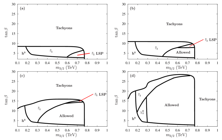
Figure 7: The viable parameter space (Allowed) opens up as $\phi$ is increased with $\theta=0$ fixed; (a) $\phi=\pi/2$, (b) $\phi=15\pi/32$, (c) $\phi=7\pi/16$ and (d) $\phi=3\pi/8$. The viable space for (a) has $\tilde{\tau}_{1}$ as the LSP and is therefore excluded anyway. We label the surrounding regions of parameter space with the sparticle(s) that provide the strongest constraints.

Figure 7 shows the evolution of the parameter space as we move away from T-moduli domination. The first important feature to notice from (a) is that only a very tiny patch of parameter space is allowed since the majority is forbidden by low-energy tachyons. The strongest constraints come from the lightest Higgs and stau (later lightest neutralino) experimental bounds, but the allowed region for T-moduli domination has a stau LSP and is therefore ruled out anyway by experimental constraints (e.g. searches for anomalously heavy nuclei predicted by nucleosynthesis). We observe from (a) to (d) how the inclusion of twisted moduli opens up the viable region by pushing back the stau/neutralino boundaries, lifting their degeneracy and yielding a neutralino LSP. Decreasing $\phi$ even further also pushes back the tachyon boundary to larger $m_{3/2}$, until we reach the limits considered in Section 3.2 where the experimental sparticle constraints reappear at low $m_{3/2}$.

3.4 General SUSY breaking with dilaton and moduli F-terms

In the previous sections we have observed the effects of varying $\phi$ (with $\theta=0$ fixed) on the evolution of the viable parameter space. We have seen that both twisted and untwisted moduli dominated limits have severely constrained parameter spaces that can be enlarged by including the effects from the other moduli F-term. We can predict that the least constrained models are likely to involve both types of moduli contributions (and also dilaton effects), and in this section we will briefly study two sample points with non-zero $\theta$, $\phi$ Goldstino angles.

3.4.1 Twisted moduli domination with dilaton and moduli F-terms: $\theta=\phi=0.1$

We will first study a point close to the twisted moduli domination limit with $\theta=\phi=0.1$, where we include additional contributions from the dilaton and untwisted moduli F-terms. The GUT-scale soft masses are given in Table 5.

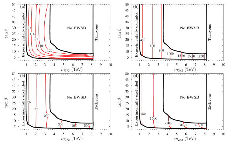
Figure 8: Maps of viable parameter space and mass contours of (a) lightest Higgs $h^{0}$, (b) gluino $\tilde{g}$, (c) neutralino $\chi_{1}^{0}$ and (d) lightest stop $\tilde{t}_{1}$ for $\theta=\phi=0.1$.

Soft mass/trilinear	(in $m_{3/2}$ units)	Soft mass/trilinear	(in $m_{3/2}$ units)
1st/2nd family $C^{5_{1}5_{2}}$	1.135	$M_{1}$	0.154
3rd family $C^{5_{2}}_{1,3}$	0.995	$M_{2}$	0.113
Higgses $C^{5_{2}}_{2}$	0.985	$M_{3}$	0.085
Trilinear $A_{C^{5_{2}}_{1}C^{5_{2}}_{2}C^{5_{2}}_{3}}$	-0.0993

Table 5: Numerical value of soft SUSY breaking parameters (in units of $m_{3/2}$ with $\alpha_{GUT}\approx 1/25$) for $\theta=\phi=0.1$.

Comparing the results shown in Figure 8 with Figure 6 (d) we conclude that there is only a very weak dependence on $\theta$. In terms of constraints, the main differences to the twisted moduli dominated limit are the range of allowed $\tan\beta$ values and the presence of tachyons at large $m_{3/2}$. The lightest Higgs limit provides the only experimental constraint at low $\tan\beta$ and small $m_{3/2}$. This model point allows heavier particles, for example the lightest Higgs $h^{0}$ can be as heavy as $120$ GeV.

3.4.2 Vanishing soft Higgs mass: $\theta=\arcsin(1/\sqrt{3})$, $\phi=0.1$

We will now study an interesting model point where the Higgs doublet soft mass vanishes at the GUT-scale by choosing $\theta=\arcsin(1/\sqrt{3})$, as shown by Eq.(20). We set $\phi=0.1$ to avoid first/second family ($C^{5_{1}5_{2}}$) tachyonic soft masses. The numerical values of the corresponding soft parameters are given in Table 6.

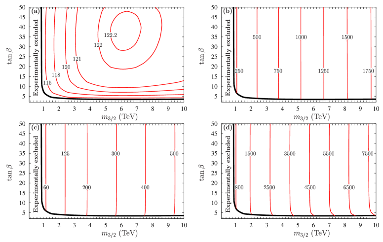
Figure 9: Maps of viable parameter space and mass contours of (a) lightest Higgs $h^{0}$, (b) gluino $\tilde{g}$ and (c) neutralino $\chi_{1}^{0}$ and (d) stop $\tilde{t}_{1}$ for $\theta=\arcsin(1/\sqrt{3})$ , $\phi=0.1$ where the soft Higgs doublet mass vanishes at the GUT-scale.

Soft mass/trilinear	(in $m_{3/2}$ units)	Soft mass/trilinear	(in $m_{3/2}$ units)
1st/2nd family $C^{5_{1}5_{2}}$	0.839	$M_{1}$	0.126
3rd family $C^{5_{2}}_{1,3}$	0.997	$M_{2}$	0.093
Higgses $C^{5_{2}}_{2}$	0	$M_{3}$	0.069
Trilinear $A_{C^{5_{2}}_{1}C^{5_{2}}_{2}C^{5_{2}}_{3}}$	-0.082

Table 6: Numerical value of soft SUSY breaking parameters (in units of $m_{3/2}$ with $\alpha_{GUT}\approx 1/25$) for $\theta=\arcsin(1/\sqrt{3})$, $\phi=0.1$.

The viable parameter space and sparticle mass contours are shown in Figure 9. It is clear that the vanishing soft mass for the Higgs doublets does not restrict the allowed space, and the only constraint originates from the lightest Higgs (and also chargino) experimental bounds at low values of $\tan\beta$ and $m_{3/2}$. The vanishing Higgs mass ensures that there are no regions ruled out by the EWSB constraints, and also tachyonic scalars do not exclude regions with large $m_{3/2}$. The sparticle mass contours take similar values to the previously studied model points, except that the lightest stop can now be much heavier, and the lightest Higgs can reach $m_{h^{0}}\approx 122$ GeV.

3.5 Comments on Flavour Changing Neutral Current constraints

One of the most appealing features of sequestered models is the geometrical explanation for the suppression of flavour changing processes due to negligible direct tree-level couplings between Standard Model and SUSY breaking fields. Using EFT techniques, we find that the contributions from non-renormalisable higher dimensional operators are exponentially-suppressed by the separation $r$ between branes and the UV cutoff scale $\Lambda_{UV}$ after integrating out the high-scale physics. In fact the dominant contributions to flavour changing off-diagonal mass-matrix elements in these parallel-brane models arise from loop corrections involving bulk fields. Therefore the squarks and sleptons start out almost massless at the GUT-scale, and receive soft masses at low energy only through RGE running effects involving the gauge couplings which couple in a flavour-blind way, leading to universal soft mass matrices at the low scale. The same mechanism suppresses the first/second family FCNCs in the twisted moduli domination limit of our SI$\tilde{g}$M model. The separation of the third family fields with a heavier soft scalar mass is allowed since the third family FCNCs are only weakly constrained by experiment. In fact a heavier third family at low-energies proves helpful in achieving successful EWSB and a sufficiently heavy lightest CP-even Higgs mass.

It is common to parameterise the amount of flavour violation using the mass-insertion (MI) approximation. In this work we have generalised the CP-conserving constraints on the MI deltas  derived from experiment in Ref. [33] to test the viability of our model for various $\theta$–$\phi$ points. The results of comparing the predicted MI deltas with the experimental limits for these points is shown in Table 7.

Ratio $R[\delta]=\delta_{SS}/\delta_{exp}$	$\theta=\phi=0$		$\theta=\phi=0.1$	$\theta=0.615,\,\phi=0.1$
Weak-scale mixing	up	down	up	up
$R[(\delta^{d}_{11})_{LR}]$	$(5.4-5.1)\times 10^{-3}$	$(5.4-5.1)\times 10^{-3}$	$(5-3.7)\times 10^{-4}$	$(6-4)\times 10^{-4}$
$R[(\delta^{d}_{22})_{LR}]$	$(6.3-6)\times 10^{-3}$	$(5.6-5.2)\times 10^{-3}$	$(6-4.4)\times 10^{-4}$	$(7-4.6)\times 10^{-4}$
$R[(\delta^{d}_{12})_{LL}]$	$(7-3.5)\times 10^{-2}$	$0.3-0.1$	$(1.6-0.4)\times 10^{-3}$	$(1.2-0.3)\times 10^{-3}$
$R[(\delta^{d}_{12})_{LR}]$	$(6-1.5)\times 10^{-7}$	$(6-1.5)\times 10^{-7}$	$(1-0.04)\times 10^{-8}$	$(1.5-0.05)\times 10^{-8}$
$R[\sqrt{(\delta^{d}_{12})_{LL}(\delta^{d}_{12})_{RR}}]$	$(2-0.8)\times 10^{-4}$	$6.5-3.5$	$(2-0.1)\times 10^{-6}$	$(5-0.2)\times 10^{-6}$
$R[(\delta^{u}_{12})_{LL}]$	$0.1-0.05$	$(3-1)\times 10^{-4}$	$(5-0.8)\times 10^{-4}$	$(5-0.5)\times 10^{-4}$
$R[(\delta^{u}_{12})_{LR}]$	$(8-1)\times 10^{-9}$	$(8-1)\times 10^{-9}$	$(3-0.15)\times 10^{-5}$	$(5-0.2)\times 10^{-5}$
$R[\sqrt{(\delta^{u}_{12})_{LL}(\delta^{u}_{12})_{RR}}]$	$0.8-0.45$	$(1-0.5)\times 10^{-7}$	$(7-1)\times 10^{-4}$	$(1-0.1)\times 10^{-3}$
$R[(\delta^{d}_{23})_{LL}]$	$(3-0.7)\times 10^{-3}$	$(8-2)\times 10^{-3}$	$(1-0.03)\times 10^{-3}$	$(1-0.02)\times 10^{-3}$
$R[(\delta^{d}_{23})_{LR}]$	$(2-0.3)\times 10^{-5}$	$(2-0.3)\times 10^{-5}$	$(5-0.1)\times 10^{-5}$	$(1-0.01)\times 10^{-4}$

Table 7: Ranges of the ratio $R[\delta]=\delta_{SS}/\delta_{exp}$ of mass-insertion deltas for the three different $\theta$–$\phi$ model points in sections 3.1, 3.4.1 and 3.4.2, with weak-scale mixing in either the up or down-quark sectors. The ranges come from scanning over allowed points in the $\tan\beta$–$m_{3/2}$ plane.

Recall from Ref. [33] that each CP-conserving flavour changing observable is calculable in terms of combinations of MI deltas, e.g. $\Delta m_{K}$ from $K^{0}$–$\overline{K}^{0}$ mixing and BR($b\longrightarrow s\,\gamma$). Assuming no accidental cancellations we can use experimental bounds to calculate upper limits on each separate MI delta as functions of the physical squark and gluino masses. For every $\tan\beta$–$m_{3/2}$ point within the allowed parameter space, we can calculate the ratio $R[\delta]=\delta_{SS}/\delta_{exp}$ between the actual MI delta matrix element $\delta_{SS}$ (calculated by SOFTSUSY) and the corresponding experimental limit $\delta_{exp}$, where regions with a ratio greater that unity are ruled out. In Figure 10 we plot contours of the ratio $R[\delta]$ for two particular delta matrix elements with weak-scale mixing in the up-quark sector - $(\delta^{u})_{LL}$ and $\sqrt{(\delta^{u}_{12})_{LL}\,(\delta^{u}_{12})_{RR}}$ - in the limit of twisted moduli domination, that are very close to being excluded by experiment. We obtain similar plots for the other MI deltas, and also for the $\theta=\phi=0.1$ and $\theta=0.615,\phi=0.1$ model points, and the relative ratios $R[\delta]$ are compared in Table 7. We also include the ratios for the twisted moduli domination limit, but with weak-scale mixing shifted to the down-quark sector.

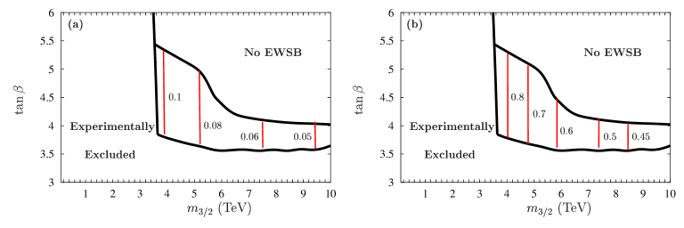
Figure 10: The ratio between mass-insertion deltas predicted by SOFTSUSY (with weak-scale mixing in the up-quark sector only) against the bounds deduced from experiment [33] for $\theta=\phi=0$: (a) $(\delta^{u}_{12})_{LL}$, (b) $\sqrt{(\delta^{u}_{12})_{LL}(\delta^{u}_{12})_{RR}}$ are closest to being ruled out or probed by experiment.

We observe that the model points (with weak-scale mixing in the up-quark sector) in Table 7 easily satisfy the experimental constraints with ranges of ratios $R[\delta]\ll 1$. We have already discussed that the mechanism for suppressing FCNCs in the twisted moduli limit is analogous to the $\tilde{g}$MSB models. However there is a different mechanism at work that solves the SUSY flavour problem when we move away from twisted moduli domination since the inclusion of gravitational SUSY breaking effects spoils the sequestering to give non-negligible first/second family soft sfermion masses at the high-scale. The suppression of FCNCs can be understood by studying the expressions for the soft parameters in Eqs.(17-26) and observing how the MI deltas vary with different gluino and first/second family squark masses [33]. For example, the diagonal soft mass-squared $m_{C^{5_{1}5_{2}}}^{2}$ for the first/second family squarks grows rapidly with increasing $\phi$ since the first term in the second line of Eq.(18) dominates. Also the gluino mass increases as the first term in Eq.(21) dominates, and a heavier gluino leads to heavier weak-scale squarks through RGE running. The heavier gluino and squark masses, in combination with the assumption of family-diagonal soft scalar mass-matrices at the high-scale, are sufficient to suppress the first/second family FCNCs and ameliorate the SUSY flavour problem.

The values of the ratios $R[\delta]$ given in Table 7 for the twisted moduli domination limit are shown to have an explicit dependence on whether the weak-scale boundary conditions for the quark Yukawa matrix parameters are imposed in the up or down-quark sectors, although the physical sparticle masses remain unaffected. For instance if the weak-scale mixing occurs exclusively in the down-quark sector, then the mixing induced in the up-quark sector should be relatively small since the up Yukawa has more effect on the up-squarks. Comparing the relative ratios $R[\delta]$ for the twisted moduli domination limit in Table 7, we see that moving the weak-scale Yukawa mixing into the down-quark sector has little effect on the mixed-parity MI deltas – $(\delta^{d}_{11})_{LR}$, $(\delta^{2}_{22})_{LR}$, $(\delta^{d}_{12})_{LR}$, $(\delta^{u}_{12})_{LR}$ and $(\delta^{d}_{23})_{LR}$ – but greatly affects the same-parity MI deltas (although $(\delta^{d}_{23})_{LL}$ only slightly changes). The main effect is to weaken the constraints on $(\delta^{u}_{12})_{LL}$ and $\sqrt{(\delta^{u}_{12})_{LL}\,(\delta^{u}_{12})_{RR}}$, that are close to experimental limits with up-quark sector mixing as shown in Figure 10, but strengthen the constraints on the equivalent down sector MI deltas $(\delta^{d}_{12})_{LL}$ and $\sqrt{(\delta^{d}_{12})_{LL}\,(\delta^{d}_{12})_{RR}}$. In fact, the value for $\sqrt{(\delta^{d}_{12})_{LL}\,(\delta^{d}_{12})_{RR}}$ implies that the twisted moduli limit is ruled out by experiment, albeit with weak-scale mixing only in the down-quark sector.

3.6 Parameter scans over $\theta$–$\phi$

In this section we will study the $\theta$–$\phi$ dependence of our SI$\tilde{g}$M model for different choices of $\tan\beta$ and $m_{3/2}$. The unitarity of the Goldstino angle parameterisation in Eq.(7) - where $F_{S}^{2}+\sum_{i}F_{T_{i}}^{2}+F_{Y_{2}}^{2}={\mathbf{F}}^{2}$ - enables us to plot points in the square $\theta$–$\phi$ parameter space as points within a triangle  with sides labelled by $\sin^{2}(\theta)$ and $\sin^{2}(\phi)$, where each triangle vertex corresponds to a particular limit of SUSY breaking as shown in Figure 11.

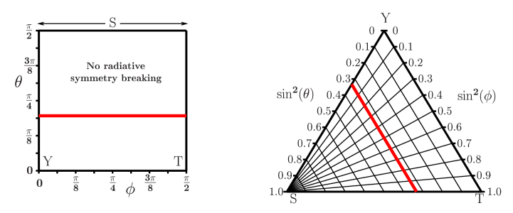
Figure 11: Generic points within the square $\theta$–$\phi$ parameter space (left panel) can be mapped on to a triangular coordinate system $\sin^{2}(\theta)$–$\sin^{2}(\phi)$ (right panel). The region above/left of the thick (red) line is forbidden since there is no radiative EWSB as the symmetry is already broken at the GUT-scale by tachyonic Higgs doublet soft scalar masses. We also label the different limits of SUSY breaking domination ($S,T,Y$) which correspond to the vertices of the triangle.

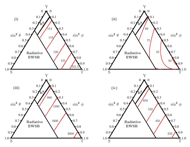
Figure 12: Sparticle mass contours (in GeV) for $m_{3/2}=700$ GeV and $\tan\beta=5$: (i) lightest higgs $h^{0}$, (ii) neutralino $\chi_{1}^{0}$, (iii) gluino $\tilde{g}$ and (iv) stau $\tilde{\tau}_{1}$. The excluded regions are marked, and there is also a tiny area close to untwisted moduli domination ($\sin^{2}\,\phi\approx 1.0$) where $\tilde{\tau}_{1}$ is the LSP.

Therefore for a generic choice of $\theta$ and $\phi$ (away from any domination limit), the relative contributions from each closed string F-term can be easily determined by measuring the perpendicular distance of the $\theta$–$\phi$ point away from each side of the triangle. Note that many earlier studies have not considered twisted moduli contributions to SUSY breaking, and so these analyses are constrained to the $S-T$ base of the triangle in Figure 11.

We have studied the allowed parameter spaces for various combinations of $m_{3/2}$–$\tan\beta$ and sparticle mass contours are shown in Figures 12-14. We plot the (i) lightest higgs $h^{0}$, (ii) neutralino $\chi_{1}^{0}$, (iii) gluino $\tilde{g}$ and lightest squark/slepton state which is either the (iv) stau $\tilde{\tau}_{1}$ or stop $\tilde{t}_{1}$. In Figure 12 we observe that the viable $\theta$–$\phi$ parameter space for $m_{3/2}=700$ GeV, $\tan\beta=5$ - which is not already forbidden by radiative symmetry breaking - is only weakly constrained, although the region with $\sin^{2}\phi\stackrel{{\scriptstyle<}}{{{}_{\sim}}}0.3$ does not predict a sufficiently heavy Higgs $h^{0}$. Also there is a small region around the T-moduli domination limit ($\sin^{2}\theta\approx 0$, $\sin^{2}\phi\approx 1$) where the lightest stau state $\tilde{\tau}_{1}$ is the LSP and is ruled out by experimental constraints. This is consistent with the results shown in Figure 7 (a).

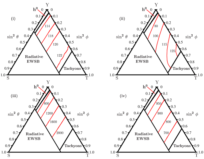
Figure 13: Sparticle mass contours (in GeV) for $m_{3/2}=1$ TeV and $\tan\beta=5$: (i) lightest higgs $h^{0}$, (ii) neutralino $\chi_{1}^{0}$, (iii) gluino $\tilde{g}$, (iv) stau $\tilde{\tau}_{1}$. The region with small $\phi$ is excluded by the experimental Higgs bound, and large $\phi$ points are ruled out by weak-scale tachyons.

Comparing Figures 12 and 13 demonstrates that even a slight increase in $m_{3/2}$ can significantly reduce the parameter space by truncating the viable region at larger values of $\phi$ due to the presence of weak-scale tachyons. Also the experimental Higgs bound becomes less constraining since it is pushed to smaller $\phi$. The range of viable Higgs and gluino masses is unaffected by the increase in $m_{3/2}$, although the positions of the contours in $\theta$–$\phi$ space are shifted. However the neutralinos and squark/slepton sparticles can be much heavier, and the lightest squark/slepton state is typically the stau . There are also regions with small $\sin^{2}\phi\stackrel{{\scriptstyle<}}{{{}_{\sim}}}0.1-0.2$ in Figures 12 and 13 where the stop squark mass is comparable to the stau.

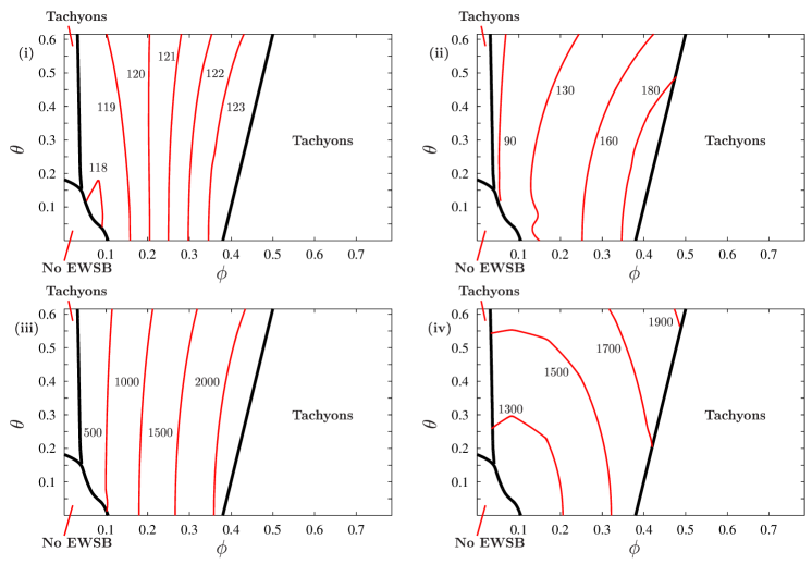
Figure 14: Sparticle mass contours (in GeV) for $m_{3/2}=2$ TeV and $\tan\beta=20$: (i) lightest higgs $h^{0}$, (ii) neutralino $\chi_{1}^{0}$, (iii) gluino $\tilde{g}$ and (iv) stop $\tilde{t}_{1}$. Note that we are using a reduced $\phi$ scale.

When $m_{3/2}$ is raised further, we see that the viable parameter space becomes increasingly narrow as weak-scale tachyons sweep in from large $\phi$. The small $\phi$ experimental Higgs $h^{0}$ limit is replaced by another tachyon boundary, and a region opens up around $\sin^{2}\theta$, $\sin^{2}\phi\approx 0$ where EWSB does not occur. We also observe that the gross features of the viable parameter space (for a given $m_{3/2}$) are not affected by increasing $\tan\beta$, except that the no EWSB region grows with increasing $\tan\beta$. Also note that for $m_{3/2}=1$ TeV, the effect of increasing $\tan\beta$ replaces the Higgs $h^{0}$ bound in Figure 13 by a similar bound from the lightest chargino $\chi_{1}^{0}$ and gluino $\tilde{g}$ sparticles.

In Figure 14 we find that the viable parameter space for $m_{3/2}=2$ TeV, $\tan\beta=20$ is too small to represent within the triangular framework, so we adopt the square $\theta$–$\phi$ coordinates with a reduced $\phi$ axis. The allowed space is constrained by low-energy tachyons at both large and small $\phi$, and also in the region around $\theta,\phi=0$ where EWSB does not occur. The larger value of $\tan\beta$ allows the neutralino $\chi_{1}^{0}$ and squark/slepton masses to be much heavier. The stop $\tilde{t}_{1}$ is now definitely lighter than the stau $\tilde{\tau}_{1}$ state, but it is still very heavy $m_{\tilde{t}_{1}}\sim{\cal O}(m_{3/2})$.

3.7 Benchmarks

Recently there have been many studies of “benchmark” points that highlight particular characteristics within a model parameter space . In Table 8 we list some sparticle spectra for our own set of benchmark points. Point A is the twisted moduli domination limit of section 3.1, and we also list the more general points B and C from section 3.4 where the dilaton and moduli F-terms each contribute to SUSY breaking. The full outputs for these three sample points can be found on

http://allanach.home.cern.ch/allanach/benchmarks/int.html

in the Les Houches Accord output format [38] to enable future Monte-Carlo analyses.

Point	A	B	C
$\theta$	0	0.1	0.615
$\phi$	0	0.1	0.1
$m_{3/2}$	5000	2000	2000
$\tan\beta$	4	10	20
$m_{h^{0}}$	114.7	117.1	118.9
$m_{A^{0}}$	5233	1991	1500
$m_{H^{0}}$	5233	1996	1528
$m_{H^{\pm}}$	5234	1992	1513
$m_{\tilde{\chi}_{1}^{0}}$	98.5	123	104
$m_{\tilde{\chi}_{2}^{0}}$	273	179	155
$m_{\tilde{\chi}_{1}^{\pm}}$	98.5	178	155
$m_{\tilde{g}}$	586	509	428
$m_{\tilde{t}_{1}}$	3061	1196	1549
$m_{\tilde{t}_{2}}$	4182	1668	1789
$m_{\tilde{c}_{1}}$, $m_{\tilde{u}_{1}}$	470	2314	1716
$m_{\tilde{c}_{2}}$, $m_{\tilde{u}_{2}}$	482	2318	1719
$m_{\tilde{b}_{1}}$	4189	1666	1780
$m_{\tilde{b}_{2}}$	5019	2002	1977
$m_{\tilde{s}_{1}}$, $m_{\tilde{d}_{1}}$	476	2314	1716
$m_{\tilde{s}_{2}}$, $m_{\tilde{d}_{2}}$	478	2319	1721
$m_{\tilde{\tau}_{1}}$	4999	1978	1947
$m_{\tilde{\tau}_{2}}$	5000	1989	1983
$m_{\tilde{\mu}_{1}}$, $m_{\tilde{e}_{1}}$	150	2273	1681
$m_{\tilde{\mu}_{2}}$, $m_{\tilde{e}_{2}}$	239	2276	1684
$m_{\tilde{\nu}_{e}}$, $m_{\tilde{\nu}_{\mu}}$	131	2275	1682
$m_{\tilde{\nu}_{\tau}}$	4999	1988	1975
LSP	$\tilde{\chi}_{1}^{0}$	$\tilde{\chi}_{1}^{0}$	$\tilde{\chi}_{1}^{0}$

Table 8: Sample spectra: All masses are in GeV and the Goldstino angles are given in radians. The high-scale input soft parameter can be found in Tables 3,5 and 6 by multiplying by $m_{3/2}$.

4 Discussion and Conclusions

The original parallel-brane models of sequestering [9, 10] have many appealing features for supersymmetric phenomenology. They offer an attractive and simple realisation of traditional hidden-sector models by localising the Standard Model and SUSY breaking sectors at opposite ends of a higher-dimensional bulk spacetime. A sequestered Kähler potential, reminiscent of no-scale SUGRA models [11], predicts that there are no direct couplings between the two sectors at leading order. Non-renormalisable higher-dimensional operators can be constructed that are found to give only exponentially small contributions using EFT techniques. Therefore the dominant contributions to the soft masses and trilinears arise from radiative corrections involving bulk fields. The absence of significant couplings may alleviate the supersymmetric flavour problem since small off-diagonal squark/slepton mass-matrix elements arise at the weak-scale through calculable RGE running effects. Unfortunately the simplest models of sequestering have severely constrained parameter spaces, and there have been recent concerns that the sequestered Kähler potential is unnatural in realistic string constructions [12].

This motivated us to propose a string-inspired gaugino mediation model of sequestering with twisted moduli [13, 14] to tackle these problems. We have attempted to put sequestering on a firmer theoretical basis by embedding it in a type I construction involving intersecting D-branes, where localised closed string twisted moduli play the rôle of the SUSY breaking sector that can be spatially-separated away from open string matter fields. We proposed a modified Kähler potential for the intersection states representing MSSM fields [14] that attributes the sequestering suppression factor (in the limit of twisted moduli domination) to non-perturbative instanton effects involving strings stretching between different fixed points [27]. As we have discussed in this paper, there are additional sources of SUSY breaking from the dilaton and untwisted T-moduli states that can be interpreted as gravity mediated SUSY breaking, and we have used a Goldstino angle [15]-[17] parameterisation to control the relative contributions to the overall SUSY breaking. This parameterisation has allowed us to move away smoothly from the sequestered limit – where only the twisted moduli contribute to SUSY breaking – and study the interplay between sequestering and gravity mediation by including the dilaton/T-moduli contributions.

In this paper we have studied the twisted moduli domination limit, where we have observed that the Higgs mass is light due to restricted $\tan\beta$ from the EWSB constraint, and where the large third family soft scalar masses yield a characteristic “stop-heavy MSSM” sparticle spectrum. In this case we have found a wino-dominated LSP which results in quasi-degenerate lightest charginos and neutralinos, leading to an opportunity, as well as difficulties in the detection of charginos [39]. We have also considered additional contributions from the untwisted T-moduli to the twisted moduli limit, and seen that the bounds on $\tan\beta$ become relaxed allowing for a larger region of viable parameter space, where the extra contributions destroy the quasi-degeneracy between chargino and neutralino. We have seen that the converse is also true, namely that the twisted moduli domination limit is strongly constrained by the tachyons, but adding T-moduli contributions considerably opens up the parameter space. We also study a particular mixed point with contributions from both the dilaton and moduli sectors that predicts a vanishing Higgs doublet soft mass at the GUT-scale without coming into conflict with empirical bounds, and we find that the lightest stop can become very heavy.

The experimental constraints from FCNC processes are satisfied within our model by two different mechanisms. Firstly in the twisted moduli domination limit, it is important to emphasise that the first two squark and slepton families have approximately zero soft masses at the high energy scale due to sequestering. This leads to a natural suppression of the most dangerous flavour changing neutral currents involving the first two families. The reason is that, at low energies, diagonal soft masses are generated for the first two families via RGE effects proportional to gauge couplings which are flavour blind, resulting in a universal form for the low energy soft mass matrices for the first and second family squarks and sleptons proportional to the unit matrix. This mechanism is very similar to that which operates in the original $\tilde{g}$MSB scenario, however unlike that scenario, where all three families of squarks and sleptons have approximately zero soft masses at the high energy scale, here this applies to only the first two families. Nevertheless this proves sufficient to suppress the most dangerous FCNCs associated with the first two families as our results in section 3.5 demonstrate.

The second mechanism suppresses FCNCs when we include gravity mediation effects to move away from twisted moduli domination. We observe that the viable parameter space rapidly increases and yields heavy sparticle masses. However the additional contributions to SUSY breaking also spoil the sequestering such that first and second family soft scalar masses are no longer negligible at the high-scale, and the FCNCs cannot be suppressed as before. Instead the heavier gluino and squark masses ameliorate the SUSY flavour problem with the additional assumption of family-diagonal sfermion mass matrices (in the weak-basis) at the high-scale. In Table 7, we see that some of the MI deltas $(\delta^{u}_{12})_{LL}$ and $\sqrt{(\delta^{u}_{12})_{LL}(\delta^{u}_{12})_{RR}}$ are within a factor of a few to 100 of being probed by experiment when we assume that the weak-scale Yukawa mixing occurs exclusively in the up-quark sector. If we change this assumption and move the mixing into the down-quark sector, we find that the previous $\delta^{u}_{12}$ values are reduced while the equivalent $\delta^{d}_{12}$ MI deltas become larger. In fact this new value for $\sqrt{(\delta^{d}_{12})_{LL}(\delta^{d}_{12})_{RR}}$ effectively rules out the twisted moduli domination limit, albeit with weak-scale mixing exclusively in the down-quark sector.

To summarise, we have performed a first phenomenological analysis of the phenomenology of twisted moduli in type I string theory. Within this framework we have discussed a string inspired version of gaugino mediated supersymmetry breaking where only the third squark and slepton family feels directly the supersymmetry breaking effects of the twisted moduli, and is therefore predicted to be significantly heavier than the first two squark and slepton families which are massless at high energies in the twisted moduli domination limit. More generally we have considered the smooth interpolation between such sequestered scenarios and gravity-mediated scenarios, by switching on the supersymmetry breaking effects of non-twisted moduli such as $S$ and $T_{i}$ in addition to the twisted moduli $Y_{2}$, which opens up the parameter space considerably. If SUSY is discovered at the LHC it will be interesting to see if the spectrum of superpartners corresponds to any of the general type I spectra including the new sequestered effects of twisted moduli considered in this paper.

Note Added

During the final stages of this paper, a phenomenological study [40] appeared on the archive which considers lighter SUSY breaking masses for the first two families. There, it is shown how the lighter two families can reconcile $(g-2)_{\mu}$, dark matter and $b\longrightarrow s\gamma$ constraints compared to the usual universal minimal SUGRA assumption. There is little overlap with the present paper except for the heavier third family sfermions, but we note that their conclusions should qualitatively apply to our model also, adding support to it.

Appendix A Derivation of the SUSY breaking F-terms

In this appendix we will show how the SUSY breaking F-terms are derived in terms of Goldstino angles using a series expansion in inverse powers of $T_{2}+\overline{T}_{2}$. We follow the analysis in Refs. [22, 23], but generalised to three untwisted moduli $T_{i}$ and $D5_{i}$-branes. Recall that the Kähler potential for the dilaton and moduli (after suppressing $M_{\ast}$) is:

$$K(S,\overline{S},T_{i},\overline{T_{i}},Y_{2},\overline{Y_{2}})=-\ln(S+\overline{S})-\sum_{i=1}^{3}\ln(T_{i}+\overline{T_{i}})+\hat{K}$$ (29)

where we choose to leave the precise form of the twisted moduli Kähler potential as an unknown function $\hat{K}\equiv\hat{K}(X)$ with an argument $X=Y_{2}+\overline{Y_{2}}-\delta_{GS}\,{\mathrm{l}n}(T_{2}+\overline{T_{2}})$ required to cancel modular anomalies [24]. The mixing induced between $T_{2}$ and $Y_{2}$ by this unknown Kähler potential means that the Kähler metric is no longer diagonal (if we ignore open string matter fields). In order to invert the Kähler metric $K_{\overline{J}\,I}$ (where $I,J=S,T_{i},Y_{2}$ label derivatives), we invoke the unitarity relation

$$P^{\dagger}\,K_{\overline{J}\,I}\,P=1$$ (30)

where the matrix $P$ canonically normalises $K_{\overline{J}\,I}$.

From Eq.(29), we obtain the following non-zero entries in the Kähler metric:

$$K_{\overline{S}\,S}=\frac{1}{(S+\overline{S})^{2}}\hskip 17.07164pt,\hskip 17.07164ptK_{\overline{T_{i}}\,T_{i}}=\frac{1}{(T_{i}+\overline{T_{i}})^{2}}\hskip 11.38109pt(i=1,3)\hskip 17.07164pt,\hskip 17.07164ptK_{\overline{Y_{2}}\,Y_{2}}=\hat{K}^{\prime\prime}\hskip 17.07164pt$$ (31)

$$K_{\overline{T_{2}}\,T_{2}}=\frac{1}{(T_{2}+\overline{T_{2}})^{2}}\left[1+\delta_{GS}\hat{K}^{\prime}+\delta_{GS}^{2}\hat{K}^{\prime\prime}\right]\hskip 17.07164pt,\hskip 17.07164ptK_{\overline{Y_{2}}\,T_{2}}=K_{\overline{T_{2}}\,Y_{2}}=-\frac{\delta_{GS}}{T_{2}+\overline{T_{2}}}\,\hat{K}^{\prime\prime}$$

where $\hat{K}^{\prime}$ ($\hat{K}^{\prime\prime}$) means the first (second) derivative with respect to the argument $X=Y_{2}+\overline{Y_{2}}-\delta_{GS}\,{\mathrm{l}n}(T_{2}+\overline{T_{2}})$.

The full Kähler metric is:

$$K_{\bar{J}I}=\left(\begin{array}[]{ccccc}\frac{1}{(S+\overline{S})^{2}}&0&0&0&0\\ 0&\frac{1}{(T_{1}+\overline{T_{1}})^{2}}&0&0&0\\ 0&0&\frac{1}{(T_{2}+\overline{T_{2}})^{2}}\left(k+\delta_{GS}^{2}\right)&0&-\frac{\delta_{GS}}{T_{2}+\overline{T_{2}}}\\ 0&0&0&\frac{1}{(T_{3}+\overline{T_{3}})^{2}}&0\\ 0&0&-\frac{\delta_{GS}}{T_{2}+\overline{T_{2}}}&0&\hat{K}^{\prime\prime}\end{array}\right)$$ (37)

where $I=S,T_{i},Y_{2}$ and for convenience we have introduced the unphysical parameter $k$ which is given by:

$$k=(T_{2}+\overline{T_{2}})^{2}K_{\overline{T_{2}}\,T_{2}}-\delta_{GS}^{2}=1+\delta_{GS}\,\hat{K}^{\prime}$$ (38)

where we have made a simplifying assumption and set $\hat{K}^{\prime\prime}=1$ in agreement with Refs. [22, 23].

Using the standard relation between F-terms, gravitino mass and the matrix $P$ [17], we define the F-terms using Goldstino angles as:

$$F_{I}\equiv\left(\begin{array}[]{c}F_{S}\\ F_{T_{1}}\\ F_{T_{2}}\\ F_{T_{3}}\\ F_{Y_{2}}\end{array}\right)=\sqrt{3}\,m_{3/2}\,P\left(\begin{array}[]{c}\sin\theta\\ \cos\theta\,\sin\phi\,\Theta_{1}\\ \cos\theta\,\sin\phi\,\Theta_{2}\\ \cos\theta\,\sin\phi\,\Theta_{3}\\ \cos\theta\,\cos\phi\\ \end{array}\right)$$ (49)

where $\theta$ and $\phi$ are Goldstino angles, $\sum_{i}\Theta_{i}^{\dagger}\Theta_{i}=1$ and we have not included any CP-phases.

Using Eqs.(30) and (37), we obtain an expression for the matrix $P$ that can be expanded for large values of ($T_{2}+\overline{T}_{2}$) to give:

$$P=\left(\begin{array}[]{ccccc}S+\overline{S}&0&0&0&0\\ 0&T_{1}+\overline{T}_{1}&0&0&0\\ 0&0&\frac{T_{2}+\overline{T}_{2}}{\sqrt{k}}&0&-\frac{\delta_{GS}}{T_{2}+\overline{T}_{2}}\\ 0&0&0&T_{3}+\overline{T}_{3}&0\\ 0&0&\frac{\delta_{GS}}{\sqrt{k}}+\frac{\sqrt{k}\delta_{GS}}{(T_{2}+\overline{T}_{2})^{2}}&0&1-\frac{\delta_{GS}^{2}}{(T_{2}+\overline{T}_{2})^{2}}\end{array}\right)+{\mathcal{O}}\left[\frac{1}{(T_{2}+\overline{T}_{2})^{3}}\right]\hskip 14.22636pt$$ (55)

which leads to the following SUSY breaking F-terms from Eq.(49):

$$F_{S} = \sqrt{3}m_{3/2}\sin\theta\,(S+\overline{S})$$

$$F_{T_{1}} = \sqrt{3}m_{3/2}\cos\theta\sin\phi\,\Theta_{1}\,(T_{1}+\overline{T}_{1})$$

$$F_{T_{2}} = \sqrt{3}m_{3/2}\cos\theta\left[\sin\phi\frac{(T_{2}+\overline{T}_{2})}{\sqrt{k}}\,\Theta_{2}-\cos\phi\,\frac{\delta_{GS}}{T_{2}+\overline{T}_{2}}\right]$$ (56)

$$F_{T_{3}} = \sqrt{3}m_{3/2}\cos\theta\sin\phi\,\Theta_{3}\,(T_{3}+\overline{T}_{3})$$

$$F_{Y_{2}} = \sqrt{3}m_{3/2}\cos\theta\left[\sin\phi\left(\frac{\delta_{GS}}{\sqrt{k}}+\frac{\sqrt{k}\delta_{GS}}{(T_{2}+\overline{T}_{2})^{2}}\right)\Theta_{2}+\cos\phi\left(1-\frac{\delta_{GS}^{2}}{(T_{2}+\overline{T}_{2})^{2}}\right)\right]$$

where $F_{T_{2}}$ and $F_{Y_{2}}$ are expanded up to ${\mathcal{O}}\left[\frac{1}{(T_{2}+\overline{T}_{2})^{3}}\right]$ and $k=1+\delta_{GS}\,\hat{K}^{\prime}$. Notice that setting $\delta_{GS}=0$ removes the mixing between $T_{2}$ and $Y_{2}$ to recover the standard F-term expressions of Ref. [17].

Appendix B Phenomenological problems with “pure” $\tilde{g}$MSB

In this appendix we will consider the original $\tilde{g}$MSB model within our D-brane setup involving three degenerate families sequestered away from SUSY breaking along an extra dimension [10]. It is well known that the $\tilde{g}$MSB scenarios are severely constrained, and we would like to see if the additional contributions from the dilaton and untwisted moduli (gravity mediation) offer a solution. Instead we observe that sequestering the third family leads to severe problems that effectively rule out “pure” $\tilde{g}$MSB within our SI$\tilde{g}$M framework.

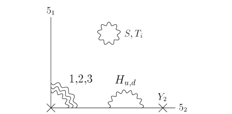
Figure 15: The allocation of open and closed string states in a string-inspired $\tilde{g}$MSB model of the MSSM. The three degenerate MSSM families ($1,2,3$) are localised at the intersection $C^{5_{1}5_{2}}$, and the Higgs doublets $H_{u,d}$ are identified as $C^{5_{2}}_{3}$ states.

Our starting point is a string-inspired model with all three MSSM families localised at the intersection region between D5-branes as shown in Figure 15, where the MSSM gauge group is once more dominated by the components on the D$5_{2}$-brane in the single-brane dominance limit. In order to have at least a top Yukawa coupling at (renormalisable) leading order, we choose the following assignment of MSSM states:

$$Q_{iL}\,,\,L_{iL}\,,\,U_{iR}^{c}\,,\,D_{iR}^{c}\,,\,E_{iR}^{c} \equiv C^{5_{1}5_{2}}\hskip 28.45274pt(i=1,2,3)$$ (57)

$$H_{u}\,,\,H_{d} \equiv C^{5_{2}}_{3}$$

which yields a democratic Yukawa texture from the allowed superpotential term

$$W_{ren}=C^{5_{2}}_{3}\,C^{5_{1}5_{2}}\,C^{5_{1}5_{2}}$$ (58)

In order to compare with the earlier analysis with only two sequestered families, we will assume that some (unspecified) flavour symmetry allows us to rotate the democratic texture into hierarchical form with a single universal non-zero (33) entry.

$\bullet$ Soft Parameters:

We follow the same arguments as section 2.1.1 to calculate the soft parameters that provide GUT-scale boundary conditions for the RGE analysis. We will assume that the universal squark and slepton mass-squared matrices are diagonal in family space at the high-scale:

$$m_{\tilde{Q}}^{2}\,,\,m_{\tilde{L}}^{2}\,,\,m_{\tilde{u}}^{2}\,,\,m_{\tilde{d}}^{2}\,,\,m_{\tilde{e}}^{2}=\left(\begin{array}[]{ccc}m_{C^{5_{1}5_{2}}}^{2}&0&0\\ 0&m_{C^{5_{1}5_{2}}}^{2}&0\\ 0&0&m_{C^{5_{1}5_{2}}}^{2}\end{array}\right)$$ (62)

where the universal scalar mass-squared $m_{C^{5_{1}5_{2}}}^{2}$ is given by Eq.(18). The Higgs doublets soft scalar mass-squared are also universal at the high-scale:

$$m_{H_{u}}^{2}\,,\,m_{H_{d}}^{2}\equiv m_{C^{5_{2}}_{3}}^{2}=m_{3/2}^{2}\left(1-\cos^{2}\theta\,\sin^{2}\phi\right)$$ (63)

The soft gaugino masses remain unchanged from Eq.(21). However the soft trilinear takes a more complicated form, and we still impose a (33) hierarchical texture:

$$A^{f}_{ij}\,Y^{f}_{ij}=\left(\begin{array}[]{ccc}0&0&0\\ 0&0&0\\ 0&0&\hat{{\cal A}}\,Y^{f}_{33}\end{array}\right)\hskip 28.45274pt(f=u,d,e)$$ (67)

where $Y^{f}_{33}$ is the (33) element of the (running) Yukawa matrix $Y^{f}$ at the GUT-scale and the universal soft trilinear $\hat{{\cal A}}$ is:

$$\hat{{\cal A}}\equiv A_{C^{5_{2}}_{3}C^{5_{1}5_{2}}C^{5_{1}5_{2}}}=-m_{3/2}\cos\theta\left[\sin\phi\left(1+\frac{X^{2}}{12}\,e^{-(T_{2}+\bar{T}_{2})/4}\,(T_{2}+\bar{T}_{2})\right)\right.\hskip 56.9055pt$$ (68)

$$+\left.\frac{2X}{\sqrt{3}}\,\cos\phi\,\left(1-e^{-(T_{2}+\bar{T}_{2})/4}\right)\right]+{\cal O}\left[\frac{\delta_{GS}\,X\,e^{-(T_{2}+\bar{T}_{2})/4}}{(T_{2}+\overline{T_{2}})}\right]$$

where $X=Y_{2}+\overline{Y_{2}}-\delta_{GS}\,{\mathrm{l}n}(T_{2}+\overline{T_{2}})$.

$\bullet$ Phenomenological problems with a large trilinear:

Following the gauge coupling unification arguments in section 2.1.2 and the choice of parameters in Table 1, we find that the soft trilinear is numerically:

$$\hat{{\cal A}}\approx-m_{3/2}\cos\theta\left[\sin\phi+45\cos\phi\right]$$ (69)

where the higher-order terms in Eq.(68) can be safely neglected. Notice that this soft trilinear has an additional (large) piece $\sim(\cos\theta\cos\phi)$ in contrast to the trilinear in Eq.(26), and we will show that this extra piece leads to problems with sfermion tachyons.

For example, we will focus on the stop sector in the limit of twisted moduli domination ($\theta,\,\phi=0$) where the trilinear is non-zero $\hat{{\cal A}}\approx-45\,m_{3/2}$. Assuming negligible intergenerational scalar mixing, the tree-level stop mass-squared eigenvalues $m_{\tilde{t}_{1,2}}^{2}$ are found by diagonalising the following $2\times 2$ mass-squared matrix ${\cal M}_{\tilde{t}}^{2}$ in the $(\tilde{t}_{L}\,\,\tilde{t}_{R})^{T}$ basis:

$${\cal M}_{\tilde{t}}^{2}=\left(\begin{array}[]{cc}\left(m_{\tilde{Q}}^{2}\right)_{33}+m_{t}^{2}+\ldots&m_{t}\left(\hat{{\cal A}}-\mu\,\cot\beta\right)\\ \vrule height=18.0pt,width=0.0ptm_{t}\left(\hat{{\cal A}}-\mu\,\cot\beta\right)&\left(m_{\tilde{u}}^{2}\right)_{33}+m_{t}^{2}+\ldots\end{array}\right)$$ (72)

where we have dropped $M_{Z^{0}}^{2}$ terms; $m_{t}$ is the physical top quark mass; and $\left(m_{\tilde{Q}}^{2}\right)_{33}\,,\,\left(m_{\tilde{u}}^{2}\right)_{33}=m_{C^{5_{1}5_{2}}}^{2}$ from Eq.(62). The determinant of Eq.(72) is the product of the mass-squared eigenvalues:

$$m_{\tilde{t}_{1}}^{2}\,m_{\tilde{t}_{2}}^{2}=\left(m_{C^{5_{1}5_{2}}}^{2}+m_{t}^{2}\right)^{2}-m_{t}^{2}\left(\mu-\hat{{\cal A}}\,\cot\beta\right)^{2}+\ldots$$ (73)

which will be negative if $\hat{{\cal A}}$ is too large (as happens here). This implies that the scalar potential involves a tachyon mass term that rules out the parameter space.

In order to avoid these tachyon problems, we must reduce the magnitude of $\hat{{\cal A}}$, and in particular the factor:

$$\frac{2}{\sqrt{3}}\,\left(1-e^{-(T_{2}+\bar{T}_{2})/4}\right)\left[Y_{2}+\overline{Y_{2}}-\delta_{GS}\,{\mathrm{l}n}(T_{2}+\overline{T_{2}})\right]\approx 45$$ (74)

when we input the parameter choices from Table 1 into Eq.(68). Our choice of $(Y_{2}+\overline{Y}_{2})=0$ and $(T_{2}+\overline{T}_{2})=50$ are motivated by gauge coupling unification in the single-brane dominance limit; the reliability of the series expansion of F-terms in Eq.(56); and we also need a sufficiently large value of $(T_{2}+\overline{T}_{2})$ for sequestering. There is some flexibility in the choice of $\delta_{GS}$, and reducing its value will indeed lower $\hat{{\cal A}}$. However the effect is not enough to make the matrix-determinant in Eq.(73) positive since all three families of sfermions are sequestered with exponentially-suppressed masses.

In contrast, the original parallel-brane $\tilde{g}$MSB models [10] do have viable regions of parameter space with sequestered squark/slepton masses, vanishing trilinears and gauginos/Higgses soft masses $\sim{\cal O}(m_{3/2})$. However in our framework the gauginos are too light to help, although they can be made heavier by increasing $\delta_{GS}$, but we already know that this will aggravate the tachyon problem further by increasing the trilinear $\hat{{\cal A}}$.

We must conclude that “pure” $\tilde{g}$MSB (in the twisted moduli domination limit) is not viable within the D-brane setup shown in Figure 15 and the choice of model parameters given in Table 1. An alternative solution may be to introduce contributions from the dilaton and untwisted moduli sectors, but we find that this requires large Goldstino angles $\theta,\phi\stackrel{{\scriptstyle>}}{{{}_{\sim}}}0.5$. We could also consider different allocations of open string states, but this also leads to problems. For instance, we could choose to sequester the Higgs doublets on the D$5_{1}$-brane with the three MSSM families kept as intersection states $C^{5_{1}5_{2}}$. The dominant top Yukawa coupling can arise from a term in the renormalisable superpotential $W_{ren}\sim C^{5_{1}}_{3}\,C^{5_{1}5_{2}}\,C^{5_{1}5_{2}}$ which automatically forbids R-parity violating superpotential terms at leading order. Unfortunately the asymmetric compactification with $R_{5_{2}}\gg R_{5_{1}}$ – that allows gauge coupling unification on the D$5_{2}$-brane – implies that $g_{5_{2}}^{2}\ll g_{5_{1}}^{2}$, and so the Higgs doublets will have a different coupling in comparison to the other MSSM fields that may be non-perturbative.

Therefore we conclude that it is very difficult to have a viable model of “pure” $\tilde{g}$MSB with three degenerate, sequestered MSSM families within our framework. Finally recall that realistic type I models do not predict three degenerate, intersection state families, but instead distinguish the third family as either $5_{1}$ or $5_{2}$ states [19].

References

- [1] A. Font, L. E. Ibanez, D. Lust and F. Quevedo, Phys. Lett. B 249 (1990) 35; M. J. Duff and J. X. Lu, Nucl. Phys. B 357 (1991) 534; A. Sen, Int. J. Mod. Phys. A 9 (1994) 3707 [arXiv:hep-th/9402002].
- [2] C. M. Hull and P. K. Townsend, Nucl. Phys. B 438 (1995) 109 [arXiv:hep-th/9410167]; E. Witten, Nucl. Phys. B 443 (1995) 85 [arXiv:hep-th/9503124].
- [3] For a review, see: J. Polchinski, arXiv:hep-th/9611050; C. V. Johnson, arXiv:hep-th/0007170.
- [4] I. Antoniadis, Phys. Lett. B 246 (1990) 377; J. D. Lykken, Phys. Rev. D 54 (1996) 3693 [arXiv:hep-th/9603133].
- [5] K. R. Dienes, E. Dudas and T. Gherghetta, Phys. Lett. B 436 (1998) 55 [arXiv:hep-ph/9803466]; Nucl. Phys. B 537 (1999) 47 [arXiv:hep-ph/9806292].
- [6] For recent reviews, see: V. A. Rubakov, Phys. Usp. 44 (2001) 871 [Usp. Fiz. Nauk 171 (2001) 913] [arXiv:hep-ph/0104152]; Y. A. Kubyshin, arXiv:hep-ph/0111027.
- [7] M. Quiros, arXiv:hep-ph/0302189.
- [8] P. Horava and E. Witten, Nucl. Phys. B 460 (1996) 506 [arXiv:hep-th/9510209]; E. Witten, Nucl. Phys. B 471 (1996) 135 [arXiv:hep-th/9602070]; P. Horava and E. Witten, Nucl. Phys. B 475 (1996) 94 [arXiv:hep-th/9603142].
- [9] L. Randall and R.Sundrum, Nucl. Phys. B 557 (1999) 79 [arXiv:hep-th/9810155].
- [10] D. E. Kaplan, G. D. Kribs and M. Schmaltz, Phys. Rev. D 62 (2000) 035010 [arXiv:hep-ph/9911293]; Z. Chacko, M. A. Luty, A. E. Nelson and E. Ponton, JHEP 0001 (2000) 003 [arXiv:hep-ph/9911323].
- [11] J. R. Ellis, K. Enqvist and D. V. Nanopoulos, Phys. Lett. B 147 (1984) 99; J. R. Ellis, C. Kounnas and D. V. Nanopoulos, Nucl. Phys. B 247 (1984) 373.
- [12] A. Anisimov, M. Dine, M. Graesser and S. Thomas, Phys. Rev. D 65 (2002) 105011 [arXiv:hep-th/0111235]; JHEP 0203 (2002) 036 [arXiv:hep-th/0201256].
- [13] K. Benakli, Phys. Lett. B 475 (2000) 77 [arXiv:hep-ph/9911517].
- [14] S. F. King and D. A. J. Rayner, JHEP 0207 (2002) 047 [arXiv:hep-ph/0111333]; arXiv:hep-ph/0211242.
- [15] A. Brignole, L. E. Ibanez and C. Munoz, Nucl. Phys. B 422 (1994) 125 [Erratum-ibid. B 436 (1995) 747] [arXiv:hep-ph/9308271]; A. Brignole, L. E. Ibanez, C. Munoz and C. Scheich, Z. Phys. C 74 (1997) 157 [arXiv:hep-ph/9508258].
- [16] A. Brignole, L. E. Ibanez and C. Munoz, arXiv:hep-ph/9707209.
- [17] L. E. Ibanez, C. Munoz and S. Rigolin, Nucl. Phys. B 553 (1999) 43 [arXiv:hep-ph/9812397].
- [18] For example, S. P. Martin, arXiv:hep-ph/9709356; D. J. H. Chung, L. L. Everett, G. L. Kane, S. F. King, J. Lykken and L. T. Wang, arXiv:hep-ph/0312378.
- [19] G. Shiu and S. H. H. Tye, Phys. Rev. D 58 (1998) 106007 [arXiv:hep-th/9805157].
- [20] S. F. King and D. A. J. Rayner, Nucl. Phys. B 607 (2001) 77 [arXiv:hep-ph/0012076].
- [21] B. C. Allanach, Comput. Phys. Commun. 143 (2002) 305 [arXiv:hep-ph/0104145].
- [22] S. A. Abel, B. C. Allanach, F. Quevedo, L. Ibanez and M. Klein, JHEP 0012 (2000) 026 [arXiv:hep-ph/0005260].
- [23] B. C. Allanach, D. Grellscheid and F. Quevedo, JHEP 0205 (2002) 048 [arXiv:hep-ph/0111057]; D. Grellscheid, arXiv:hep-ph/0304277.
- [24] L. E. Ibanez, R. Rabadan and A. M. Uranga, Nucl. Phys. B 542 (1999) 112 [arXiv:hep-th/9808139].
- [25] S. A. Abel and G. Servant, Nucl. Phys. B 597 (2001) 3 [arXiv:hep-th/0009089]; Nucl. Phys. B 611 (2001) 43 [arXiv:hep-ph/0105262].
- [26] T. Higaki and T. Kobayashi, Phys. Rev. D 68 (2003) 046006 [arXiv:hep-th/0304200]; T. Kobayashi and O. Seto, Phys. Rev. D 69 (2004) 023510 [arXiv:hep-ph/0307332]; T. Higaki, Y. Kawamura, T. Kobayashi and H. Nakano, arXiv:hep-ph/0308110.
- [27] S. Hamidi and C. Vafa, Nucl. Phys. B 279 (1987) 465; L. J. Dixon, D. Friedan, E. J. Martinec and S. H. Shenker, Nucl. Phys. B 282 (1987) 13; L. E. Ibanez, Phys. Lett. B 181 (1986) 269.
- [28] S. F. King and I. N. R. Peddie, arXiv:hep-ph/0312237.
- [29] E. Poppitz, Nucl. Phys. B 542 (1999) 31 [arXiv:hep-th/9810010]; C. A. Scrucca and M. Serone, JHEP 0007 (2000) 025 [arXiv:hep-th/0006201];
- [30] G. G. Ross and O. Vives, Phys. Rev. D 67 (2003) 095013 [arXiv:hep-ph/0211279].
- [31] S. F. King and I. N. R. Peddie, Nucl. Phys. B 678 (2004) 339 [arXiv:hep-ph/0307091].
- [32] G. L. Kane and S. F. King, Phys. Lett. B 451 (1999) 113 [arXiv:hep-ph/9810374]; M. Bastero-Gil, G. L. Kane and S. F. King, Phys. Lett. B 474 (2000) 103 [arXiv:hep-ph/9910506].
- [33] F. Gabbiani, E. Gabrielli, A. Masiero and L. Silvestrini, Nucl. Phys. B 477 (1996) 321 [arXiv:hep-ph/9604387].
- [34] K. Hagiwara et al. [Particle Data Group Collaboration], Phys. Rev. D 66 (2002) 010001.
- [35] G. L. Fogli, E. Lisi, A. Marrone and G. Scioscia, Phys. Rev. D 59 (1999) 033001 [arXiv:hep-ph/9808205].
- [36] B. C. Allanach et al., in Proc. of the APS/DPF/DPB Summer Study on the Future of Particle Physics (Snowmass 2001) ed. N. Graf, Eur. Phys. J. C 25 (2002) 113 [eConf C010630 (2001) P125] [arXiv:hep-ph/0202233].
- [37] G. L. Kane, J. Lykken, S. Mrenna, B. D. Nelson, L. T. Wang and T. T. Wang, Phys. Rev. D 67 (2003) 045008 [arXiv:hep-ph/0209061].
- [38] P. Skands et al. arXiv:hep-ph/0311123.
- [39] A. J. Barr, C. G. Lester, M. A. Parker, B. C. Allanach and P. Richardson, JHEP 0303 (2003) 045 [arXiv:hep-ph/0208214].
- [40] H. Baer, A. Belyaev, T. Krupovnikas and A. Mustafayev, arXiv:hep-ph/0403214.