CP asymmetry in $B\rightarrow\phi K_{S}$ in a general two-Higgs-doublet model with fourth-generation quarks

Abstract

We discuss the time-dependent CP asymmetry of decay $B\rightarrow\phi K_{S}$ in an extension of the Standard Model with both two Higgs doublets and additional fourth-generation quarks. We show that although the Standard Model with two-Higgs-doublet and the Standard model with fourth generation quarks alone are not likely to largely change the effective $\sin 2\beta$ from the decay of $B\rightarrow\phi K_{S}$, the model with both additional Higgs doublet and fourth-generation quarks can easily account for the possible large negative value of $\sin 2\beta$ without conflicting with other experimental constraints. In this model, additional large CP violating effects may arise from the flavor changing Yukawa interactions between neutral Higgs bosons and the heavy fourth generation down type quark, which can modify the QCD penguin contributions. With the constraints obtained from $b\rightarrow s\bar{s}s$ processes such as $B\rightarrow X_{s}\gamma$ and $\Delta m_{B_{s}^{0}}$, this model can lead to the effective $\sin 2\beta$ to be as large as $-0.4$ in the CP asymmetry of $B\rightarrow\phi K_{S}$.

I introduction

With the successful running of two $B$ factories in KEK and SLAC, precise measurements of the time-dependent CP asymmetries as well as the directly CP asymmetries in rare $B$ decays become available. Among those interesting decay modes, the most important one, the CP asymmetry of $B\rightarrow J/\psi K_{S}$ has been successfully measured, and a very good agreement with the Standard Model (SM) prediction on $\sin 2\beta$ was found.

However, the recent Belle results on $\sin 2\beta$ from $B\rightarrow\phi K_{S}$, although with significant errors, have indicated that the value of $\sin 2\beta$ from different decay modes could be significantly different. The most recent measurements give Abe et al. (2003a); Aubert et al. (2004)

$$\sin 2\beta = 0.47\pm 0.34^{+0.08}_{-0.06}(\operatorname{Babar}),$$

$$\sin 2\beta = -0.96\pm 0.5^{+0.09}_{-0.11}(\operatorname{Belle}).$$ (1)

Of course, it is too early to draw any robust conclusion from the current preliminary data. Nevertheless, it opens a possibility that large new physics effects may show up in the $b\rightarrow sss$ processes, which has already triggered a large amount of theoretical efforts in examining the possible new physics contributions from various models. Besides the models related to supersymmetry which are the most promising ones, there are also a large class of models based on simple extensions of the matter contents of the SM, such as the standard models with two-Higgs-doublet (S2HDM) Glashow and Weinberg (1977); Savage (1991); Hou (1992); Antaramian et al. (1992); Hall and Weinberg (1993); Wu and Wolfenstein (1994); Wolfenstein and Wu (1994); Wu (1994); Atwood et al. (1997); Dai et al. (1997); Bowser-Chao et al. (1999); Diaz et al. (2000); Zhou and Wu (2000); Xiao et al. (2002); Wu and Zhou (2001); Zhou and Wu (2003) and the standard model with fourth-generation fermions (SM4)Chou et al. (1984); Datta and Paschos (1989); Huang et al. (2001, 1999); Arhrib and Hou (2003) etc. However, the most recent studies have pointed out that the contributions from the above mentioned two types of models to $B\rightarrow\phi K_{S}$ are in general not large enough to account for a large negative value of $\sin 2\beta$ in $B\rightarrow\phi K_{S}$ ( for example $\sin 2\beta\approx-0.5$ ) Hiller (2002); Giri and Mohanta (2003); Huang and Zhu (2003); Arhrib and Hou (2003).

In this paper, we show that although due to the constraints from other experiments such as $b\rightarrow s\gamma$ and $\Delta m_{B}$ etc., the general S2HDM and the SM4 alone are not likely to largely change the effective $\sin 2\beta$ in $B\rightarrow\phi K_{S}$, a model with both an additional Higgs doublet and 4th-generation quarks (denoted by S2HDM4) can significantly change the value of $\sin 2\beta$ without contradicting with other experimental constraints. In this model, new large CP violating contributions may arise from the flavor-changing Yukawa interactions between the neutral Higgs boson and the 4th-generation down type quark $b^{\prime}$ (with $m_{b^{\prime}}\gg m_{b}$), which changes the Wilson coefficients for QCD penguin operators and results in a large modification of effective $\sin 2\beta$. This mechanism is different from the case in the S2HDM in which the dominant contribution comes from changing the Wilson coefficients of the electro(chromo)-magnetic operators. The latter is subjected to a rather strong constraint from $b\rightarrow s\gamma$ and therefore can not give enough contributions.

Let us begin with some model independent discussions. The definition of effective $\sin 2\beta$ in $B\rightarrow\phi K_{S}$ is

$$\sin 2\beta_{\operatorname{eff}} = \operatorname{Im}\left[e^{2i\beta}\frac{\bar{\mathcal{A}}}{\mathcal{A}}\right]=\operatorname{Im}\left[e^{2i\beta}\frac{\bar{\mathcal{A}}_{\operatorname{SM}}(1+re^{-i\theta})}{\mathcal{A}_{\operatorname{SM}}(1+re^{+i\theta})}\right],$$ (2)

where $\beta$ is the SM value with $\sin 2\beta=0.715^{+0.055}_{-0.045}$ Buras (2002). $\bar{\mathcal{A}}_{\operatorname{SM}}(\mathcal{A}_{\operatorname{SM}})$ is the SM value of the decay amplitude of $\overline{B}^{0}(B^{0})\rightarrow\phi K_{S}$. Here two parameters $r$ and $\theta$ parameterize the relative size and the additional CP violating phase of the new physics contributions. To get an idea of how $\sin 2\beta_{\operatorname{eff}}$ is changes with the new physics contribution, we take some typical values of the phase $\theta$, calculate the values of $\sin 2\beta_{\operatorname{eff}}$, and shown them in Fig.1.

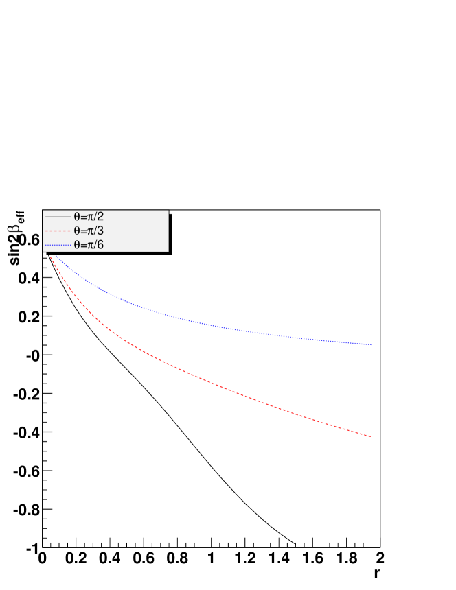
Figure 1: The value of $\sin 2\beta_{\operatorname{eff}}$ as a function of $r$. The solid, dashed and dotted curves corresponds to $\theta=\pi/2,\pi/3$ and $\pi/6$ respectively.

As it is shown in the figure, to explain the possibly large negative $\sin 2\beta_{\operatorname{eff}},$ for instance, close to $-0.5$, in the case that $\theta$ is maximum ($\pi/2$), the value of $r$ should be close to unity. For smaller $\theta$ such as $\pi/3$ and $\pi/6$, the value of $r$ must be even larger. Therefore, to generate a large negative value of $\sin 2\beta_{eff}$ in the range of $-0.5\sim-1.0$, the magnitude of the new physics contributions must be as the same order of magnitude as the one in the SM.

However, the new physics contributions must be constrained by other experiments, especially by the $b\rightarrow s$ transition related processes. The most strict constraint comes from the radiative decay of $B\rightarrow X_{s}\gamma$. The current data of $\operatorname{Br}(B\rightarrow X_{s}\gamma;E_{\gamma}>1.6\operatorname{GeV})=(3.28^{+0.41}_{-0.36})\times 10^{-4}$ Barate et al. (1998); Chen et al. (2001); Abe et al. (2001); Aubert et al. (2002) is well reproduced in the frame work of the next-to-leading order calculations in the SM (see e.g.Gambino and Misiak (2001); Buras et al. (2002)). Thus, if the new physics contribution carries no new phase, there is very little room for the new physics parameters. But in the case that new phases present, the parameter space could be enlarged. This is because the data of $B\rightarrow X_{s}\gamma$ only constraints the absolute values of the Wilson coefficient $C_{7\gamma}$ , if the new physics contribution does not change the absolute value of $C_{7\gamma}$, there will not be a serious problem. Thus the following relation must be satisfied for any new physics model

$$\left.\left.\left.\left.\right|C_{7\gamma}\right|=\left|C_{7\gamma}^{\operatorname{SM}}+C_{7\gamma}^{\operatorname{NEW}}\right|\simeq\right|C_{7\gamma}^{\operatorname{SM}}\right|,$$ (3)

with $C_{7\gamma}^{\operatorname{SM}}$ and $C_{7\gamma}^{\operatorname{NEW}}$ being the effective Wilson coefficient evaluated at the low energy scale $(\mu\approx m_{b})$ from SM and new physics models respectively. In this case, the absolute value of $C_{7\gamma}^{\operatorname{NEW}}$ could vary largely from close to zero to about $-2\text{$C_{7\gamma}^{\operatorname{SM}}$}$, which seems large enough for explaining the CP asymmetry in $B\rightarrow\phi K_{S}$. However, it follows from Eq.(3) that the data on $B\rightarrow X_{s}\gamma$ do strongly constrain the form of $C_{7\gamma}^{\operatorname{NEW}}$, namely, the new physics must interfere in such a way that the total effect is roughly equivalent to adding a phase factor to $C_{7\gamma}^{\operatorname{SM}}$, i.e $C_{7\gamma}\simeq|C_{7\gamma}^{\operatorname{SM}}|e^{i\theta}$. Let us take an illustrative example in which the new physics contribution is purely electro(chromo)-magnetic and satisfy $C_{7\gamma}=|C_{7\gamma}^{\operatorname{SM}}|e^{i\theta}$ and also $C_{8g}=|C_{8g}^{\operatorname{SM}}|e^{i\theta}$ at the scale of $m_{W}$. Varying the value of $\theta$ from 0 to $2\pi$ and then running down to the low energy scale of $\mu\simeq m_{b}$ through renormalization group equation, one finds that the value of $\sin 2\beta_{\operatorname{eff}}$ in decay $B\rightarrow\phi K_{S}$ only changes from 0.5 to 0.8, This naive discussion shows that if the dominant contribution from a new physics model is coming from $C_{7\gamma(8g)}^{\operatorname{NEW}}$, the change to $\sin 2\beta_{\operatorname{eff}}$ from the its SM value is limited. Unfortunately, the S2HDM belongs to this class of model. The recent analysis have confirmed that within S2HDM, the value of $\sin 2\beta_{\operatorname{eff}}$ can reach zero, but not likely to be largely negativeHiller (2002); Giri and Mohanta (2003); Huang and Zhu (2003).

For the model of SM4, there are additional up ($t^{\prime}$) and down ($b^{\prime}$) type quarks. The new phases may come from the extended Cabbibo-Kobayashi-Maskawa(CKM) matrix which is a four by four matrix in this model and contains undetermined matrix elements of $V_{t^{\prime}q},V_{qb^{\prime}}$ etc. To avoid the precise data of electro-weak processes, the mass of $b^{\prime}$ ( $t^{\prime}$ ) has to be pushed to greater than $\sim$200 GeV( $\sim 300$ GeV). However, phenomenological study showed that with the constraint of $B\rightarrow X_{s}\gamma$ and $B^{0}_{s}-\overline{B^{0}}_{s}$ mixings being considered, its contribution to the CP violation of $B\rightarrow\phi K_{S}$ is not large enough eitherArhrib and Hou (2003). Thus if the large negative value of $\sin 2\beta_{eff}$ in decay $B\rightarrow\phi K_{S}$ is confirmed by the future experiments, the above mentioned two models ( i.e. S2HDM and SM4 ) will not be favored.

sectionThe model of S2HDM4

There are several directions in constructing models beyond the SM, such as enlarging the gauge groups to $\operatorname{SU}(5)$, $\operatorname{SU}(10)\operatorname{and}E_{6}$ etc., introducing new symmetries like various SUSY models, and expanding the matter contents, i.e., more fermions and Higgs bosons. The models of the last type can be regarded as simple extensions of the SM which keep the same gauge structure but still have rich sources of new contributions. The typical ones are the above mentioned S2HDM and SM4.

In this paper we would like to a step further to consider a model with both two-Higgs-doublet and fourth-generation quarks (S2HDM4). In this model, there are new Yukawa interactions between Higgs bosons and heavy fourth-generations quarks. Since in general the Yukawa interaction is expected to be proportional to the coupled quark mass, the new Yukawa couplings are much stronger than that in the S2HDM and SM4 . Unlike in the case of S2HDM, where the $b$ quark contribution to the QCD penguin diagram through neutral Higgs boson loop is strongly suppressed by the small $b$ quark mass, the same diagram with intermediate $b^{\prime}$ quark may significantly contribute to the related processes Wu (1999). This new feature only exists in this combined model, and is of particular interest in studying the CP violation of $B\rightarrow\phi K_{S}$ and other penguin dominant processes.

The Lagrangian for the S2HDM4 is given by

$$\mathcal{L}_{Y} = \bar{\psi}_{L}Y^{U}_{1}\widetilde{\phi_{1}}u_{R}+\bar{\psi}_{L}Y^{D}_{1}\phi_{1}d_{R}+\bar{\psi}_{L}Y^{U}_{2}\widetilde{\phi_{2}}u_{R}+\bar{\psi}_{L}Y^{D}_{2}\phi_{2}d_{R}+H.c$$ (4)

with the extended quark content of $u_{L,R}=(u,c,t,t^{\prime})_{L,R}$ and $d_{L,R}=(d,s,b,b^{\prime})_{L,R}$. The Yukawa coupling matrices $Y^{U(D)}_{i}$ are 4-dimensional matrices accordingly. The two Higgs fields $\phi_{1},\phi_{2}$ have vacuum expectation values (VEV) of $v_{1}e^{i\delta_{1}}$ and $v_{2}e^{i\delta_{2}}$ respectively, with $\sqrt{|v_{1}|^{2}+|v_{1}|^{2}}=v=246\operatorname{GeV}.$ The relative phase $\delta=\delta_{1}-\delta_{2}$ between two VEVs is physical and provides a new source of CP violationWu and Wolfenstein (1994); Wolfenstein and Wu (1994); Wu (1994) . In the mass eigenstates, the three physical Higgs bosons are denoted by $H^{0},A^{0},\operatorname{and}H^{\pm}$ respectively. Due to the non-zero phase $\delta$, all the Yukawa couplings become complex numbers in the physical mass basis, even they are all real in the flavor basis. For simplicity, throughout this paper, we assume that the CKM matrix elements associating with $t^{\prime}$, i.e. $V_{t^{\prime}q}$ are ignorablly small and will only focus on the neural Higgs boson contributions.

In the mass basis, the Yukawa interactions between neutral Higgs bosons and quarks have the following general form

$$\mathcal{L}_{Y} = \eta^{q}_{ij}\bar{q}_{iL}q_{jR}\phi+H.c.,$$ (5)

with $\phi=H^{0}$ or $A^{0}$. The Yukawa coupling $\eta^{q}_{\operatorname{ij}}$ is usually parameterized as

$$\eta_{\operatorname{ij}}^{q} = \frac{\sqrt{m_{q_{i}}m_{q_{j}}}}{v}\xi_{q_{i}q_{j}}$$ (6)

In the Chen-Sher ansartz Cheng and Sher (1987) motivated by a Fritzsch type of Yukawa coupling matrix. the values of all $\xi_{q_{i}q_{j}}$s are of the same order of magnitude. However, from other textures of the coupling matrix the relations among $\xi_{q_{i}q_{j}}$s are differentZhou (2003); Diaz-Cruz et al. (2004); Diaz et al. (2003). In the general case, they should be taken as free parameters to be determined or constrained by the experiments.

The effective Hamiltonian for $\Delta B=1$ charmless $B$ decays reads

$$H_{\operatorname{eff}} = \frac{G_{F}}{\sqrt{2}}\left[V_{\operatorname{ub}}V_{\operatorname{us}}^{*}(C_{1}^{u}Q_{1}^{u}+C_{2}^{u}Q_{2}^{u})+V_{\operatorname{cb}}V_{\operatorname{cs}}^{*}(C_{1}^{c}Q_{1}^{c}+C_{2}^{c}Q_{2}^{c})\right.$$ (7)

$$\left.-V_{\operatorname{tb}}V_{\operatorname{ts}}^{*}\left(\sum_{i=3}^{10}C_{i}Q_{i}+C_{7\gamma}Q_{7\gamma}+C_{8g}Q_{8g}\right)\right],$$

where the operator basis $Q_{i}$s can be found in Ref.Buras (1998). In this model, the relevant Wilson coefficients at the scale of $m_{W}$ from this model is given by

$$C_{1}(M_{W}) = \frac{11}{2}\frac{\alpha_{s}(M_{W})}{4\pi},$$

$$C_{2}(M_{W}) = 1-\frac{11}{6}\frac{\alpha_{s}(M_{W})}{4\pi}-\frac{35}{18}\frac{\alpha_{\operatorname{em}}}{4\pi},$$

$$C_{3}(M_{W}) = -\frac{\alpha_{s}(M_{W})}{24\pi}(\tilde{E}_{0}(x_{t})+|\xi_{tt}|^{2}E_{0}^{\operatorname{III}}(y)+\frac{m_{b^{\prime}}\sqrt{m_{b}m_{s}}}{2V_{tb}V_{ts}^{*}m_{t}^{2}}\xi_{bb^{\prime}}^{*}\xi_{sb^{\prime}}E_{0}^{\operatorname{III}}(y^{\prime})),$$

$$+\frac{\alpha_{\operatorname{em}}}{6\pi}\frac{1}{\sin^{2}\theta_{W}}(2B_{0}(x_{t})+C_{0}(x_{t})),$$

$$C_{4}(M_{W}) = \frac{\alpha_{s}(M_{W})}{8\pi}(\tilde{E}_{0}(x_{t})+|\xi_{tt}|^{2}E_{0}^{\operatorname{III}}(y)+\frac{m_{b^{\prime}}\sqrt{m_{b}m_{s}}}{2V_{tb}V_{ts}^{*}m_{t}^{2}}\xi_{bb^{\prime}}^{*}\xi_{sb^{\prime}}E_{0}^{\operatorname{III}}(y^{\prime})),$$

$$C_{5}(M_{W}) = -\frac{\alpha_{s}(M_{W})}{24\pi}(\tilde{E}_{0}(x_{t})+|\xi_{tt}|^{2}E_{0}^{\operatorname{III}}(y)+\frac{m_{b^{\prime}}\sqrt{m_{b}m_{s}}}{2V_{tb}V_{ts}^{*}m_{t}^{2}}\xi_{bb^{\prime}}^{*}\xi_{sb^{\prime}}E_{0}^{\operatorname{III}}(y^{\prime})),$$

$$C_{6}(M_{W}) = \frac{\alpha_{s}(M_{W})}{8\pi}(\tilde{E}_{0}(x_{t})+|\xi_{tt}|^{2}E_{0}^{\operatorname{III}}(y)+\frac{m_{b^{\prime}}\sqrt{m_{b}m_{s}}}{2V_{tb}V_{ts}^{*}m_{t}^{2}}\xi_{bb^{\prime}}^{*}\xi_{sb^{\prime}}E_{0}^{\operatorname{III}}(y^{\prime})),$$

$$C_{7\gamma}(M_{W}) = \frac{A(x_{t})}{2}-\frac{1}{2}\left(A(y)|\xi_{t}|^{2}+A(y^{\prime})\frac{m_{b^{\prime}}\sqrt{m_{b}m_{s}}}{2V_{tb}V_{ts}^{*}m_{t}^{2}}\xi_{bb^{\prime}}^{*}\xi_{sb^{\prime}}\right),$$

$$+B(y)|\xi_{t}\xi_{b}|e^{i\theta}-B(y^{\prime})\frac{m_{b^{\prime}}\sqrt{m_{b}m_{s}}}{2V_{tb}V_{ts}^{*}m_{t}m_{b}}\xi_{b^{\prime}b}\xi_{sb^{\prime}},$$

$$C_{8g}(M_{W}) = -\frac{D(x_{t})}{2}-\frac{1}{2}\left(D(y)|\xi_{t}|^{2}+D(y^{\prime})\frac{m_{b^{\prime}}\sqrt{m_{b}m_{s}}}{2V_{tb}V_{ts}^{*}m_{t}^{2}}\xi_{bb^{\prime}}^{*}\xi_{sb^{\prime}}\right),$$ (8)

$$+(y)|\xi_{t}\xi_{b}|e^{i\theta}-E(y^{\prime})\frac{m_{b^{\prime}}\sqrt{m_{b}m_{s}}}{2V_{tb}V_{ts}^{*}m_{t}m_{b}}\xi_{b^{\prime}b}\xi_{sb^{\prime}}^{*},$$

with $\alpha_{s}(m_{W})$ and $\alpha_{\operatorname{em}}$ being the strong and electro-magnetic couplings at scale $m_{W}$. The mass ratios $x_{t},y$ and $y^{\prime}$ are defined as $x_{t}=m_{t}^{2}/m_{W}^{2}$, $y=m_{t}^{2}/m_{H^{\pm}}^{2}$ and $y^{\prime}=m_{b^{\prime}}^{2}/m_{H^{0}}^{2}$ respectively. The loop integration functions are standard and can be found in Refs.Inami and Lim (1981); Gilman and Wise (1980, 1983); Xiao et al. (2002). Here we have ignored the coefficients for the electro-weak penguin diagrams since their effects are less significant in the decay of $B\rightarrow\phi K_{S}$.

Note that the new contributions to QCD and electro(chromo)-magnetic operators depends on different parameter sets. In the QCD penguin sector, the contribution depends on $\xi_{bb^{\prime}}^{*}\xi_{sb^{\prime}}$ where in electro(chromo)-magnetic sector it depends on both $\xi_{b^{\prime}b}\xi_{sb^{\prime}}$ and $\xi_{bb^{\prime}}^{*}\xi_{sb^{\prime}}$. It is convenient to define two weak phases $\theta_{1}$ and $\theta_{2}$ with

$$\xi_{bb^{\prime}}^{*}\xi_{sb^{\prime}}=|\xi_{bb^{\prime}}\xi_{sb^{\prime}}|e^{i\theta_{1}}\quad\mbox{and}\quad\xi_{b^{\prime}b}\xi_{sb^{\prime}}=|\xi_{b^{\prime}b}\xi_{sb^{\prime}}|e^{i\theta_{2}}.$$ (9)

Since in general $\xi_{b^{\prime}b}$ and $\xi_{bb^{\prime}}^{*}$ are complex numbers and $\xi_{b^{\prime}b}\neq\text{$\xi_{bb^{\prime}}^{*}$}$, the two phases are not necessary to be equivalent. The presence of two rather than one independent phases is particular for this model, which gives different contributions to the QCD penguin and electro(chromo)-magnetic Wilson coefficients. The interference between them enlarges the allowed parameter space. Note that the Wilson coefficient for QCD penguins may be complex numbers which provides additional sources of CP violation. To make a comparison, let us denote the Wilson coefficients in the SM by $C^{SM}_{i}$. Taking $\xi_{b^{\prime}b}=\xi_{sb^{\prime}}=0.8$, $\theta_{1}=0.5$, $\theta_{2}=-1.2$ and $m_{H^{0}}=m_{b^{\prime}}=200$GeV as an example, in the range of $40<\xi_{bb^{\prime}}<60$, the ratio of $C_{3}/C_{3}^{SM}(C_{4}/C_{4}^{SM})$ has an imaginary part between -0.27 and -0.4(-0.6 and -0.8). These large imaginary parts plays an important role in CP violation.

II Constraints from $B\rightarrow X_{s}\gamma$ and$B^{0}_{s}-\bar{B}^{0}_{s}$ mixing

Before making any predictions, one first needs to know how the new parameters in this model are constrained by other experiments. For the process we are concerning, the most strict constraints comes from $b\rightarrow s\bar{s}s$ processes such as $B\rightarrow X_{s}\gamma$ and $B^{0}_{s}-\bar{B}^{0}_{s}$ mixing, etc.

The expression for $B\rightarrow X_{s}\gamma$ normalized to $B\rightarrow X_{c}e\bar{\nu}_{e}$ reads

$$\frac{\operatorname{Br}(B\rightarrow X_{s}\gamma)}{\operatorname{Br}(B\rightarrow X_{c}e\bar{\nu}_{e})} = \frac{6|V_{\operatorname{tb}}V_{\operatorname{ts}}^{*}|^{2}\alpha_{\operatorname{em}}}{\pi|V_{\operatorname{cb}}|^{2}f(m_{c}/m_{b})}|C_{7\gamma}(\mu)|^{2}$$ (10)

with $f(z)=1-8z^{2}-24z^{4}\ln z+8z^{6}-z^{8}$ and $\operatorname{Br}(B\rightarrow X_{c}e\bar{\nu}_{e})=10.45\%$. The low energy scale $\mu$ is set to be $m_{b}$. Using the Wilson coefficients at the scale $m_{W}$ and running down to the $m_{b}$ scale through re-normalization group equations, we obtain the predictions for Br($B\rightarrow X_{s}\gamma$). For simplicity, we focus on the case in which the $b^{\prime}$ contribution dominates through $H^{0}$ loop, namely, we push the masses of the charged Higgs $H^{\pm}$ and the other pseudo-scalar boson $A^{0}$ to be very high $(m_{H^{\pm}},m_{A^{0}}>500$ GeV) and ignore their contributions. We take the following typical values of the couplings

$$|\xi_{bb^{\prime}}|=50,\quad|\xi_{b^{\prime}b}|=0.8,\quad|\xi_{sb^{\prime}}|=0.8,\quad\operatorname{and}\quad m_{H^{0}}=m_{b}^{\prime}=200\operatorname{GeV},$$ (11)

and give in Fig.2 the value of Br($B\rightarrow X_{s}\gamma$) as a function of $\theta_{1}$ with different values of $\theta_{2}$.

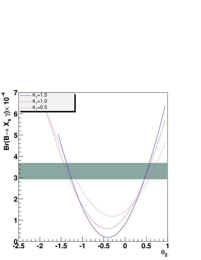
Figure 2: The branching ratio of $B\rightarrow X_{s}\gamma$ as a functions of $\theta_{2}$ in the model of S2HDM4 . The solid, dashed and dotted curves correspond to $\theta_{1}=1.5,1.0\operatorname{and}0.5$ respectively. Other parameters are taken from Eq.(11).

From the figure, one finds that two separated ranges for parameters $\theta_{1}$ and $\theta_{2}$ are allowed by the data

$$\text{$-1.4\lesssim\theta_{2}\lesssim-1.2$}\operatorname{and}\text{ $0.4\lesssim\theta_{2}\lesssim 0.7$}\qquad\operatorname{for}\text{$0.5\lesssim\theta_{1}\lesssim 1.5$},$$ (12)

Note that we do not make a scan for the full parameter space, nevertheless the above obtained range are already enough for our purpose. Among the two allowed ranges, the one with $-1.4\lesssim\theta_{2}\lesssim-1.2$ is of particular interest. It will be seen below that in this range, the contribution to the CP asymmetry in $B\rightarrow\phi K_{S}$ could be significant. In Fig.3, we also give the allowed range of $\theta_{1}$ with difference values of $\theta_{2}$. One finds that the allowed range for $\theta_{1}$ is larger compared with $\theta_{2}$. In this figure, the interference between two phases $\theta_{1}$ and $\theta_{2}$ is manifest. For $\theta_{2}$ in the range of $(-1.0,-0.8)$, the allowed value for $\theta_{1}$ is a narrow window around zero. But for $\theta_{2}$ in the range of $(-1.4,-1.2)$, the allowed range for $\theta_{1}$ could be between 0.5 and 2.0. Compared with the S2HDM in which only one phase appears, this interference effect for two phases enlarges the parameter space under the constraint of $B\rightarrow X_{s}\gamma$. Thus large contributions to the other processes is possible in this model.

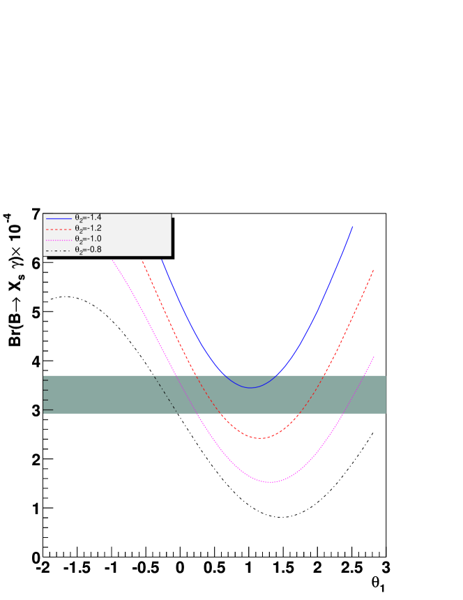
Figure 3: The branching ratio of $B\rightarrow X_{s}\gamma$ as a functions of $\theta_{1}$ in the model of S2HDM4 . The solid, dashed, dotted and dot-dashed curves correspond to $\theta_{2}=1.4,1.2,1.0\operatorname{and}0.8$ respectively. Other parameters are taken from Eq.(11)

.

The other $b\rightarrow s\bar{s}s$ process which could impose strong constraint is the mass difference of neutral $B_{s}^{0}$ meson. The measurements from LEP give a lower bound of $\Delta m_{B_{s}}>14.9ps^{-1}$. In this model, the $b^{\prime}$ contributes to $\Delta m_{B_{s}}$ only through box-diagrams. The box diagram contribution to $\Delta m_{B_{s}}$ is given by Inami and Lim (1981); Gilman and Wise (1980, 1983); Wu and Zhou (2000)

$$\Delta m_{B_{s}} = \frac{G_{F}^{2}}{6\pi^{2}}(f_{B_{s}}\sqrt{B_{B_{s}}})^{2}m_{B_{s}}m_{t}^{2}|V_{\operatorname{ts}}|^{2}\{\eta_{\operatorname{tt}}B^{\operatorname{WW}}(x_{t})+\frac{1}{4}\eta^{\operatorname{HH}}_{\operatorname{tt}}y_{t}|\xi_{tt}|^{4}B^{\operatorname{HH}}_{V}(y_{t})$$ (13)

$$+2\eta_{\operatorname{tt}}^{\operatorname{HW}}y_{t}|\xi_{\operatorname{tt}}|^{2}B^{\operatorname{HW}}_{V}(y_{t},y_{w})+\frac{1}{4}\eta^{\operatorname{HH}}_{\operatorname{tt}}y^{\prime}(\frac{m_{b^{\prime}}\sqrt{m_{b}m_{s}}}{2V_{tb}V_{ts}^{*}m_{t}^{2}}\xi_{bb^{\prime}}^{*}\xi_{sb^{\prime}})^{2}B^{\operatorname{HH}}_{V}(y^{\prime})\}$$

where $G_{F}=1.16\times 10^{-5}\operatorname{GeV}^{-2}$ is the Fermi constant. $f_{B_{s}}$ and $B_{B_{s}}$ are the decay constant and bag parameter for $B_{s}^{0}$. In the numerical calculations, we take the value of $f_{B_{s}}\sqrt{B_{B_{s}}}=0.23$GeV. $\eta_{ij}$s are the QCD correction factors. The loop integration functions of $B^{\operatorname{HH},\operatorname{WW},\operatorname{HW}}_{(V)}$ can be found in RefsGilman and Wise (1980, 1983); Wu and Zhou (2000). The mass ratios are defined as $y_{t}=m_{t}^{2}/m_{H^{\pm}}^{2},y_{w}=m_{t}^{2}/m_{W}^{2}$ and $y^{\prime}=m_{b^{\prime}}^{2}/m_{H^{0}}^{2}$ respectively. Note that in the mass difference of $B^{0}_{s}$ mesons, the contribution from S2HDM4 only depends on the parameter $\xi_{bb^{\prime}}^{*}\xi_{sb^{\prime}}$. So, only the phase $\theta_{1}$ will present in the expression.

Using the above obtained typical parameters in Eq.(11), the contribution to $\Delta m_{B_{s}}$ is calculated and plotted as a function of $\theta_{1}$ in Fig.4. The figure shows that the current data of $\Delta m_{B_{s}}$ do not impose strong constraint on the value of $\theta_{1}$.

The neutron electric dipole moment (EDM) is expected to give strong constraints on the new physics. In the SM, the neutron EDM is zero at even two loop level. The current experimental upper limit gives EDM$<1.1\times 10^{-25}ecm.$Hagiwara et al. (2002). In general, the new physics contributes to the neutron EDM through one loop diagrams. In the presence of new scalars, additional significant contributions may arise, for example from the Weinberg gluonic operator Weinberg (1989) and also the two-loop Barr-Zee type diagrams Bjorken and Weinberg (1977); Barr and Zee (1990) etc.

However, we note that all the above three type of mechenisms are not related to $b\to s$ flavor-changing transitions and therefore will involve different parameters in this model. For the one-loop diagrams, the neutral EDM is mostly related to $\xi_{u(d)}$ and $\xi_{t(b^{\prime})}$ through $u(d)-$quark EDM. For Weinberg three gluonic operator, the dominate contribution is from intereral $b^{\prime}$ loop. Thus it is related to $\xi_{b^{\prime}b^{\prime}}$. Similarly, for two-loop Barr-Zee diagram, the $b^{\prime}-$quark loop will play the most important role and the couplings involve only $\xi_{u(d)},\xi_{b^{\prime}b^{\prime}}$ etc. Thus the neutron EDM will impose strong constraints on other paramerters in this model and has less significance in current studying of decay $B\to\phi K_{S}$. This is significantly different from the S2HDM case in which the $t-$quark alway domains the loop contribution and the couplings $\xi_{tt}$ and $\xi_{bb}$ are subjected to a strong constraint from neutron EDM.

Other constraints may come from $K^{0}-\overline{K^{0}}$ and $B^{0}_{d}-\overline{B^{0}_{d}}$ mixings. But those processes contain additional free parameters such as the the Yukawa coupling of $\xi_{b^{\prime}d}$ and $\xi_{sb^{\prime}}$, the constraints from those processes are much weaker.

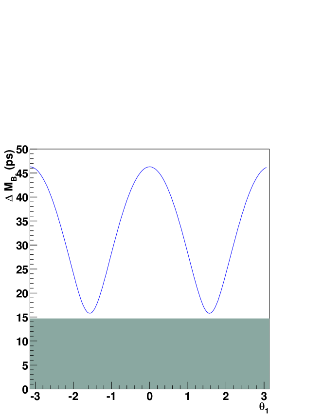
Figure 4: The $B^{0}_{s}$ meson mass difference $\Delta B^{0}_{s}$ as a function of $\theta_{1}$ in the model of S2HDM4 . Other parameters are taken from Eq.(11). The shadowed region is excluded by the data of $\Delta B^{0}_{s}$.

III CP asymmetry in $B\rightarrow\phi K_{S}$

Now we are in the position to discuss CP asymmetry in $B\rightarrow\phi K_{S}$. The decay amplitude for $\bar{B}\rightarrow\phi\bar{K^{0}}$reads

$$\mathcal{A}(\bar{B}^{0}_{d}\rightarrow\phi\bar{K}^{0}) = -\frac{G_{F}}{\sqrt{2}}V_{\operatorname{ts}}^{*}V_{\operatorname{tb}}(a_{3}+a_{4}+a_{5}-\frac{1}{2}(a_{7}+a_{9}+a_{10}))X,$$ (14)

with $X$ being a factor related to the hadronic matrix elements. In the naive factorization approach $X=2f_{\phi}m_{\phi}(\epsilon\cdot p_{B})F_{1}(m_{\phi})$, where $\epsilon$, $p_{B}$, $F_{1}$ are the polarization vector of $\phi$, the momentum of $B$ meson and form factor respectively. The coefficients $a_{i}$ are defined through the effective Wilson coefficients $C^{\operatorname{eff}}_{i}s$ as follows

$$a_{2i-1}=C^{\operatorname{eff}}_{2i-1}+\frac{1}{N_{c}}C^{\operatorname{eff}}_{2i} a_{2i}=C^{\operatorname{eff}}_{2i}+\frac{1}{N_{c}}C^{\operatorname{eff}}_{2i-1},$$ , (15)

Since the heavy particles such as $H^{\pm,0},A^{0}\operatorname{and}b^{\prime}$ has been integrated out below the scale of $m_{W}$, the procedures to obtain the effective Wilson coefficients $C^{eff}_{i}$ are exactly the same as in SM and can be found in Ref.Buchalla et al. (1996) .

Using the above obtained parameters allowed by the current data, the prediction for the time dependent CP asymmetry for $B\rightarrow\phi K_{S}$ are shown in Fig.5

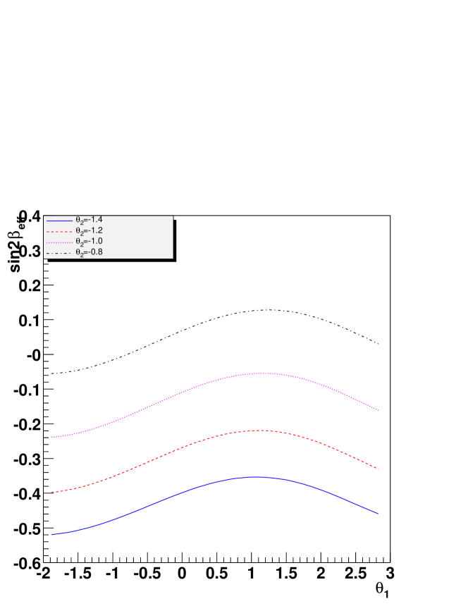
Figure 5: The prediction for $\sin 2\beta_{\operatorname{eff}}$ as a functions of $\theta_{1}$ with different value of $\theta_{2}$. The solid, dashed, dotted and dot-dashed curves corresponds to $\theta_{2}=-1.4,-1.2,-1.0,-0.8$ respectively.

In the figure, we give the value of $\sin 2\beta_{\operatorname{eff}}$ as a function of $\theta_{1}$ with different values of $\theta_{2}$=1.4,1.2,1.0 and 0.8. Comparing with the constraints obtained from $B\rightarrow X_{s}\gamma$ and $B^{0}_{s}-\bar{B}^{0}_{s}$ mixings, one sees that in the allowed range of $-1.4<\theta_{2}<-1.2$ and $0.5<\theta_{1}<1.5$, the predicted $\sin 2\beta_{\operatorname{eff}}$ can reach $-0.4$.

It is evident that the large negative value of $\sin 2\beta_{eff}$ is a consequence of the interference effects between $\theta_{1}$ and $\theta_{2}$ and therefore is particular for this model. For zero value of $\theta_{1}$, there is no new phase in the QCD penguin sector. From Fig.3, the allowed range for $\theta_{2}$ is $-1.0\lesssim\theta_{2}\lesssim-0.8$. Then, it follows from Fig.5, that in this range the predicted $\sin 2\beta_{eff}$ is at around zero. But for $\theta_{1}\approx 0.5$, the allowed range for $\theta_{2}$ is changed into $-1.4\lesssim\theta_{2}\lesssim-1.2$ and the predictions for $\sin 2\beta_{eff}$ is much lower in the range of $(-0.4,-0.25)$.

IV Conclusions

In conclusion, we have discussed the CP asymmetry of decay $B\rightarrow\phi K_{S}$, in the model of S2HDM4 which contains both an additional Higgs doublet and fourth generation quarks. In this model, since the fourth generation $b^{\prime}$ quark is much heavier that $b$ quark, the Yukawa interactions between neutral Higgs boson and $b^{\prime}$ is greatly enhanced. This results in significant modification to the QCD penguin diagrams. We have obtained the allowed range of the parameters from the process of $B\rightarrow X_{s}\gamma$ and $\Delta m_{B_{s}}$. Due to the more complicated phase effects, in this model the constraints from those process are weaker than that in S2HDM and SM4. The effective $\sin 2\beta_{\operatorname{eff}}$ in the decay $B\rightarrow\phi K_{S}$ is predicted with the constrained parameters. We have found that this model can easily account for the possible large negative value of $\sin 2\beta$ without conflicting with other experimental constraints.

In this paper we focus on the case in which $H^{0}$ domains. It is straight forward to find that the contribution from the other pseudo-scalar $A^{0}$ follows the same pattern. In the case of small mixing among the neutral scalars, the Yukawa couplings for $H^{0}$ and $A^{0}$ are directly related Atwood et al. (1997). We find that for $m_{A^{0}}\approx 200\mbox{ GeV }\ll m_{H^{0}}$ its contribution to the decay amplitude of $B\to\phi K_{S}$ is similar to the case of the $H^{0}$ dominance discussed above. For the case that $m_{A^{0}}$ is close to $m_{H^{0}}$, the contribution from them are comparable, and the interference between the two could be important.

Since this model contributes new phases to QCD penguin diagrams, it remains to be seen if it has sizable effects on other penguin dominant processes, such as in the hadronic charmless B decays. Similarly, it is expected that in this model there are also significant contributions to the electro-weak (EW) penguin diagrams which deserves a further investigation (for recent discussions on EW penguin effects on $B\to\phi K$ see, e.gAtwood and Hiller (2003); Morrissey and Wagner (2004); Deshpande and Ghosh (2003).) It is well known that the EW penguin plays important roles in rare B decays. The current data on $B\rightarrow\pi\pi,\pi K$ have indicated some deviations from results based on the SM Aubert et al. (2003); Abe et al. (2003b, 2004); Zhou et al. (2001); Wu and Zhou (2003); Buras et al. (2003). It is of interest to further investigate the new physics contributions to those decay modes within this model.