Radiative and semi-leptonic B–meson decay spectra: Sudakov resummation beyond logarithmic accuracy and the pole mass

Abstract:

The inclusive spectra of radiative and semi-leptonic B–meson decays near the endpoint is computed taking into account renormalons in the Sudakov exponent (Dressed Gluon Exponentiation). In this framework we demonstrate the factorization of decay spectra into hard, jet and soft functions and discuss the universality of the latter two. Going beyond perturbation theory the soft function, which we identify as the longitudinal momentum distribution in an on-shell b quark, is replaced by the b–quark distribution in the B meson. The two differ by power corrections. We show how the resummation of running–coupling effects can be used to perform consistent separation to power accuracy between perturbative and non-perturbative contributions. In particular, we prove that the leading infrared renormalon ambiguity in the Sudakov exponent cancels against the one associated with the definition of the pole mass. This cancellation allows us to identify the non-perturbative parameter that controls the shift of the perturbative spectrum in the heavy–quark limit as the mass difference between the meson and the quark.

1 Introduction

Inclusive B–meson decay processes, such as the semi-leptonic process $\bar{B}\longrightarrow X_{u}l^{-}{\bar{\nu}}_{l}$ and the rare $\bar{B}\longrightarrow X_{s}\gamma$ process, attract much attention in the recent years [1, 2, 3, 4, 5, 6, 7, 8, 9, 10, 11, 12, 13, 14, 15, 16, 17, 18, 19, 20, 21, 22, 23, 24, 25, 26, 27]. This is primarily because of the availability of increasingly accurate experimental data and the role of these decays in determining the parameters of the Cabbibo-Kobayashi-Maskawa (CKM) matrix as well as their potential in accessing physics beyond the standard model. Owing to experimental constraints, measurement are usually restricted to certain kinematical regions so the theoretical prediction of differential decay distributions is invaluable.

The inclusive nature of the measurement and the fact that the $b$–quark mass ($m$) is large compared to the QCD scale ($\Lambda$) guarantee infrared safety. Consequently, the b–quark decay spectra are calculable in perturbative QCD. On the other hand, the fact that the b quark is part of a bound state has a significant impact on the spectra. It has been understood long ago that the relevant non-perturbative information is contained in the longitudinal–momentum distribution of the b quark in the B meson [13]. However, the limited understanding of the properties of this distribution has been a major stumbling block in developing precision phenomenology.

The theoretical description of the spectra is particularly challenging near the endpoints, i.e. near maximal photon energy in $\bar{B}\longrightarrow X_{s}\gamma$, or near maximal charged–lepton energy in semi-leptonic decays. Describing the spectra in terms of $x\equiv 2E/M$, where $E$ is the photon (or charged–lepton) energy in the B rest frame and $M$ is the meson mass, the endpoint corresponds to the $x\longrightarrow 1$ limit. It turns out that the $x\sim 1$ region is experimentally important. This is so, in particular, for the $\bar{B}\longrightarrow X_{u}l^{-}{\bar{\nu}}_{l}$ decay which can be accurately measured only beyond the $\bar{B}\longrightarrow X_{c}l^{-}{\bar{\nu}}_{l}$ threshold.

Kinematic constrains imply that near the endpoints the hadronic final state has large energy, ${\cal O}(M)$, but small invariant mass, ${\cal O}(M\sqrt{1-x})$. Furthermore, radiation off the heavy quark has typical transverse momenta of order $M(1-x)$. Since the quark is confined in a meson this radiation is physically inseparable from interaction with the light degrees of freedom in the meson. Thus, the binding of the heavy quark, its kinetic energy as well as other properties of the bound state are probed at large $x$ where $1-x\sim{\cal O}(\Lambda/M)$.

At the perturbative level, the constrained real–emission phase space at large $x$ is reflected in appearance of Sudakov logs, $\ln(1-x)$. Such large corrections appear owing to the singularity of the parton–branching probability in the soft and the collinear limits. As a consequence, any fixed–order perturbative result diverges in the $x\longrightarrow 1$ limit although the physical distribution vanishes there. All–order resummation of the logarithmically–enhanced terms is therefore essential to recover the qualitative behaviour of the distribution near the endpoint. Sudakov resummation can indeed be performed using the standard tools of QCD factorization [28, 29, 30, 31, 32, 33, 34, 35], which is based on identifying within the multi-scale physical distribution separate subprocesses each described by a function of a single physical scale. Specifically, in inclusive decays there are three subprocesses: hard, jet and soft that are described by functions of $M$, $M\sqrt{1-x}$ and $M(1-x)$, respectively. Resummation of the logarithms is then achieved by solving perturbative evolution equations for these functions [14].

It is clear, however, that enhanced corrections appear also non-perturbatively. While for moderate $x$ power corrections appear on the scale $M$, which is significantly larger than the QCD scale $\Lambda$, at large $x$ there are enhanced corrections depending on the jet mass scale, $M\sqrt{1-x}$, and, most importantly, on the soft scale, $M(1-x)$. Since, in the region of interest, the latter is of the order of the QCD scale, one deals here with an infinite set of power corrections, which can be summed up into a non-perturbative shape function [11, 14].

Much theoretical work has already been done on inclusive B–decay spectra [1, 2, 3, 4, 5, 6, 7, 8, 9, 10, 11, 12, 13, 14, 15, 16, 17, 18, 19, 20, 21, 22, 23, 24, 25, 26, 27]. Most recent investigations [26, 27] have been based on the so-called soft collinear effective theory [36, 37, 38, 39, 40], by which factorization is implemented at the level of fields. Despite this progress there are certain theoretical questions that remain open and limit the prospects of precision phenomenology. This includes, in particular, the question of how to systematically separate between perturbative and non-perturbative corrections on the soft scale. The present work is a step in resolving this question.

The crucial observation is that for infrared and collinear safe observables in general, and for B–decay spectra in particular, the separation between perturbative and non-perturbative contributions should be based on power accuracy. This stands in contrast with the commonly used collinear factorization, which applies for example to structure functions in deep inelastic scattering, where the separation is based on logarithmic accuracy. In fact, when considering the decay spectrum near the endpoint, there is no effective way to perform logarithmic separation. Such separation would have only been effective had there been a large gap between $M(1-x)$ and $\Lambda$ such that one could have chosen a factorization scale $\mu$ which satisfies $\Lambda\ll\mu\ll M(1-x)$. In the region of interest the soft function receives perturbative and non-perturbative contributions from roughly the same momentum scales. The perturbative contributions correspond to gluon radiation off the heavy quark, radiation that peaks at transverse momentum $k_{\perp}\sim m(1-x)$. The perturbative soft function describes the longitudinal–momentum distribution of a (slightly off-shell) b quark inside an on-shell b quark. The non-perturbative contribution amounts to power–suppressed corrections which distinguish the latter from the b–quark distribution inside a B meson. Note that although the on-shell b quark is not an asymptotic state — the full quark propagator has no pole — the b–quark distribution in an on-shell b quark is well defined to any order in perturbation theory. The price one eventually pays for dealing with a non-physical object, the on-shell quark, is parametrically small: it is the power–suppressed ambiguity in the sum of perturbation theory.

This distinction between the QCD analysis of infrared and collinear safe observables and the standard, collinear factorization can be formulated also in terms of evolution. Collinear factorization is based on computing the anomalous dimension perturbatively and then supplementing the evolution equation by a purely non-perturbative initial condition. On the other hand for infrared and collinear safe observables one computes perturbatively also the initial condition and the role of non-perturbative corrections is restricted to modifying this initial condition by power terms.

Our plan is to extend the concept of large–$x$ factorization and the resulting Sudakov resummation beyond any logarithmic accuracy. In order to explain how this is done, let us first recall the standard implementation of Sudakov resummation, e.g. [16, 20, 21], and examine its limitations. It is worthwhile stressing already now that these limitations are not the consequence of a specific mathematical procedure, but instead, they are inherent to the logarithmic accuracy criterion.

It is convenient to formulate Sudakov resummation in moment space; see Eq. (8) below for a definition. The moment index $N$ is the Mellin conjugate variable to $x$, so large moments become increasingly sensitive to the interesting $x\longrightarrow 1$ limit. Owing to momentum conservation contributions of different subprocesses at large $x$ are simply written as a product in moment space. Furthermore, the factorization property of soft and collinear matrix elements implies that the soft subprocess (and likewise the jet) can be written in moment space as an exponential. The standard approach to Sudakov resummation is based on computing the moment–space exponent to a fixed logarithmic accuracy, usually next–to–leading logarithmic accuracy, thus resumming terms of the form $\alpha_{s}^{n}\ln^{k}N$ where $k=n+1$ (leading logs — LL) as well as $k=n$ (next–to–leading logs — NLL) in the exponent. This contribution can be summed over $n$ to all orders, yielding a well–defined function. Nevertheless, this function has unphysical poles (Landau singularities) at $N\sim{\cal O}(m/\Lambda)$. When converting the resummed series back to $x$ space these poles lead to large fluctuations at large $x$. The perturbative result is then unstable with respect to higher–order corrections for $x$ values between the peak and the endpoint.

While the moment–space perturbative result is well defined at any given logarithmic accuracy, the corrections owing to subleading logarithms (that are neglected) are large. Because of the sensitivity of the contributing diagrams to small momenta, subleading logarithms $k<n$ have larger numerical coefficients which eventually break the hierarchy on which the perturbative expansion is based. This is a result of infrared renormalon contributions to the Sudakov exponent [41]. Similarly to other perturbative series in QCD [42, 43], owing to infrared renormalons the Sudakov exponent is non-Borel-summable. Upon summing the perturbative expansion with no restriction on the logarithmic accuracy (i.e. on $n-k$) the exponent develops power–suppressed ambiguities. In this way resummation of running–coupling effects leads to identifying power–like ambiguities in the moment–space exponent opening up the possibility to perform separation at power accuracy between perturbative and non-perturbative corrections.

The appearance of renormalons in the Sudakov exponent is not special to B–decay spectra but is rather common to a wide range of QCD distributions near kinematic thresholds. The Dressed Gluon Exponentiation (DGE) approach deals with this situation by performing a renormalon calculation of the Sudakov exponent, defining it by an appropriate regularization prescription, such as the principal value of the Borel integral, and finally parametrizing non-perturbative corrections to the moment–space exponent based on the parametric form of the ambiguity. It is worth noting that, contrary to any fixed–logarithmic–accuracy resummation, the principal–value regularization of the Sudakov exponent has no Landau singularities. Existing applications of DGE range from event–shape distributions in the two–jet limit [41, 44], through deep inelastic structure functions at large Bjorken $x$ [45, 46, 47], to the heavy–quark fragmentation function [48] which is closely related to B decay.

Aiming at power accuracy we begin our perturbative analysis of decay spectra by performing resumming of running–coupling effects. In practice the calculation is done, as in other applications, with a single dressed gluon, i.e. to leading order in the large–$\beta_{0}$ limit. We exponentiate the $x\longrightarrow 1$ singular terms in moment space, identify the renormalon ambiguity of the Sudakov exponent and define the sum of the series by the principal value of the Borel integral, a choice that also defines the non-perturbative correction.

In the b–quark distribution analyzed here, much like the heavy–quark fragmentation function [50, 48, 49], the ambiguity of the Sudakov exponent corresponds to powers of $N\Lambda/m$. The ambiguity implies the existence of genuine non-perturbative corrections to the exponent of a similar parametric form. Independently of how these power corrections are parametrized, as soon as they become important the renormalon ambiguities of the Sudakov exponent cannot be ignored. From this perspective it is hard to interpret any phenomenological description of the non-perturbative b–quark distribution in the B meson which does not take into account the renormalons.

Deeper understanding the b-quark distribution function requires establishing the cancellation of ambiguities between its perturbative and non-perturbative ingredients. This separation is ambiguous because it is based on the concept of an on-shell heavy quark. Using the heavy quark effective theory (HQET) [51, 52] we show that the leading power correction, of order $N\Lambda/M$, cancels between the perturbative Sudakov exponent and non-perturbative corrections involving the quark pole mass [53, 54, 55, 56, 57, 58]. Defining both the Sudakov exponent and the pole mass by the same prescription (e.g. principal value of the Borel sum) the parameter that controls the corresponding non-perturbative effect on the spectrum — a shift — is uniquely identified. The final result is independent of the prescription used. This extends the previous result on cancellation of renormalon ambiguities in the total decay width [56] to the level of differential decay spectra.

The structure of this paper is as follows. In section 2 we consider the radiative $\bar{B}\longrightarrow X_{s}\gamma$ decay spectrum, present the perturbative DGE result for the moments and then consider in some detail the power–like separation between perturbative and non-perturbative contributions to the b–quark distribution. In particular, we identify the relevant non-perturbative parameters using the HQET and prove the cancellation of the first infrared renormalon ambiguity. Although we refer specifically to the radiative decay, the analysis of the b–quark distribution is general: it applies to other inclusive decays as well. In section 3, we turn to the semi-leptonic decay spectrum focusing on the analogy and differences with the radiative decay. Appendix B gives some more details of the corresponding renormalon calculation where the soft and jet functions are computed separately. Section 4 is reserved for conclusions.

2 $\bar{B}\longrightarrow X_{s}\gamma$ decay

In this section we address perturbative and non-perturbative aspects of the energy spectrum in the radiative B decay, $\bar{B}\longrightarrow X_{s}\gamma$. We begin by computing the photon energy distribution to all orders in the large–$\beta_{0}$ limit. This is done by performing the one–loop calculation with a Borel–modified gluon propagator. Next we focus on the endpoint region, first in perturbation theory and then beyond. In section 2.1.1 we compute the Sudakov exponent in moment space. We then show (section 2.1.3) that this result is consistent with factorization into hard, jet and soft functions, and match the DGE result with NLL accuracy and with the full ${\cal O}(\alpha_{s})$ result (section 2.1.4). To end the perturbative part we demonstrate in section 2.1.5 the divergence of the Sudakov exponent and analyse the difference between truncation at fixed logarithmic accuracy and principal–value resummation. Non-perturbative aspects are discussed in section 2.2, beginning, in section 2.2.1, with precise identification of the relevant power corrections (the shape function) through the moment–space ratio between the quark distribution in a meson and the one in an on-shell heavy quark. In section 2.2.2 we identify the first few parameters that control power corrections in the heavy–quark limit using the HQET and finally, in section 2.2.3, we prove the cancellation of the leading renormalon ambiguity.

Let us first define the kinematics. We denote the inclusive differential $\bar{B}\longrightarrow X_{s}\gamma$ decay rate by $\Gamma$, and define

$$x\equiv 2p_{\gamma}\cdot p_{B}/M^{2},$$

where $p_{\gamma}$ and $p_{B}$ are the photon and B–meson momentum, respectively ($p_{\gamma}^{2}=0$, $p_{B}^{2}=M^{2}$). In the $B$ rest frame $x$ represents the photon energy fraction: $x=2E_{\gamma}/M$.

The short–distance electroweak physics responsible for the decay can be integrated out yielding an effective Hamiltonian description which involves eight operators of dimension five and six [1]. Calculation of the corresponding coefficient functions, the evolution from $W$–mass scale to the $b$–quark mass scale, and perturbative evaluation of the matrix elements shows that the $\bar{B}\longrightarrow X_{s}\gamma$ decay is dominated by the following magnetic operator [4, 15, 18]:

$$H=\sqrt{2}G_{F}V_{tb}V_{ts}^{*}A(m_{t}^{2}/m_{W}^{2})\,\frac{em}{16\pi^{2}}\,\bar{s}_{L}\sigma^{\mu\nu}b_{R}F_{\mu\nu},$$ (1)

where $F_{\mu\nu}$ is the photon field strength. The contribution of this particular operator is singled out by being singular in the $x\longrightarrow 1$ limit in which we are interested. Therefore, in the following we only consider this operator. We would like to emphasise that a complete analysis needed for phenomenology would have to take into account other operators as well. There, however, the standard perturbative treatment is likely to be sufficient.

2.1 Perturbation theory

2.1.1 A renormalon calculation

Referring to the $B$ meson as if it were a free on-shell b quark, the inclusive distribution in $x$ is infrared and collinear safe, so it can be computed perturbatively in QCD. At the perturbative level the scaling variable $x$ becomes $2p_{\gamma}\cdot p/m^{2}$ where $p$ is the b–quark momentum and $m$ is the pole mass, $p^{2}=m^{2}$. A calculation of the real–emission cuts with a single dressed gluon yields the following distribution:

$$\frac{1}{\Gamma_{\hbox{\tiny total}}}\frac{d\Gamma}{dx} = (1+{\cal O}(\alpha_{s}))\delta(1-x)+\frac{C_{F}}{2\beta_{0}}\int_{0}^{\infty}du\,T(u)\,\left(\frac{\Lambda^{2}}{m^{2}}\right)^{u}\,B(x,u)$$ (2)

with

$$B(x,u) \equiv {\rm e}^{cu}\,\frac{\sin\pi u}{\pi u}\,x^{3}\,(1-x)^{-u}\int_{0}^{1}d\alpha\,\alpha\,(1-\alpha)^{-u}\,\times$$

$$\bigg{[}\frac{1}{(1-x\alpha)^{2}}\left(1-4\alpha+\alpha^{2}-\frac{(1-\alpha)^{2}}{1-u}\right)+\frac{1-\alpha}{(1-x\alpha)(1-u)}+\frac{2}{1-x}\frac{1}{1-x\alpha}+\frac{1}{1-x}\bigg{]},$$

where $\Lambda$ is in the ${\overline{\rm MS}}$ scheme and $c=5/3$.

To arrive at this result we computed the imaginary part of the three one–loop diagrams of Fig. 1 with a Borel–modified gluon propagator,

$$\frac{1}{-k^{2}}\longrightarrow\frac{(\Lambda^{2})^{u}}{(-k^{2})^{1+u}}.$$

Integrating over the Borel parameter $u$ is equivalent to resumming a gauge–invariant set of diagrams with a single dressed gluon to all orders. The set of diagrams is defined by evaluating the running coupling at the scale of the gluon virtuality,

$$\frac{\beta_{0}\alpha_{s}(-k^{2})}{\pi}=\int_{0}^{\infty}du\,T(u)\,\left(\frac{\Lambda^{2}}{-k^{2}}\right)^{u},$$ (4)

and it reduces to the insertion of an arbitrary number of fermion loops in the large–$N_{f}$ limit; see e.g. [43]. Here $\beta_{0}$ is the leading–order coefficient of the $\beta$ function,

$$\frac{d(\alpha_{s}/\pi)}{d\ln\mu^{2}}=-\beta_{0}(\alpha_{s}/\pi)^{2}-\beta_{1}(\alpha_{s}/\pi)^{3}+\ldots\hskip 60.0pt\beta_{0}=\frac{11}{12}C_{A}-\frac{1}{6}N_{f}\,,$$ (5)

and the exponential factor ${\rm e}^{cu}$ in Eq. (2.1.1) originates in the renormalization of the fermion loop in the $\overline{\rm{MS}}$ scheme. Throughout this paper we shall be using the scheme–invariant formulation [59] of the Borel transform. In the large–$\beta_{0}$ limit (one–loop running coupling) $T(u)\equiv 1$. This function is introduced here so that the running coupling can be considered beyond one loop, e.g. truncating Eq. (5) at two loops one has:

$$T(u)=\frac{(u\delta)^{u\delta}{\rm e}^{-u\delta}}{\Gamma(1+u\delta)}.$$ (6)

where $\delta=\beta_{1}/\beta_{0}^{2}$

In Eq. (2.1.1) the terms in the square brackets are written as they appear from individual diagrams in the Feynman gauge. The first two terms corresponds to gluon emission from the b quark prior to its decay (diagram I), the last (fourth) term to gluon emission from the strange quark in the final state (diagram III) and the third term to interference between the two amplitudes (diagram II).

Figure 1: The three one–loop diagrams contributing to the squared decay matrix element of a heavy quark (thick line) into a light quark (horizontal, thin line).

Upon expanding the Borel integrand near $u=0$ to leading order (${\cal O}(u^{0})$), Eq. (2) reproduces the known ${\cal O}(\alpha_{s})$ real–emission contribution to this process (cf. [15]),

$$\frac{1}{\Gamma_{\hbox{\tiny total}}}\frac{d\Gamma}{dx}=(1+{\cal O}(\alpha_{s}))\delta(1-x)$$

$$\quad+\frac{C_{F}\alpha_{s}}{2\pi}\left[-\left(1+x+\frac{2}{1-x}\right)\ln(1-x)-\frac{7}{2}\frac{1}{1-x}+\frac{7}{2}+\frac{1}{2}x-x^{2}\right].$$ (7)

Beyond this order Eq. (2) resums running–coupling effects to all orders in perturbation theory in a scheme invariant manner. In particular, renormalization–scale dependence is avoided. With $T(u)=1$ this resummation comprises at any order $n$ of the terms of the form $C_{F}\beta_{0}^{n}\alpha_{s}^{n+1}$. Using $T(u)$ this resummation is generalized to include the effects of subleading corrections to the running of the coupling.

2.1.2 Borel representation of the Sudakov exponent

The most striking feature of the $\bar{B}\longrightarrow X_{s}\gamma$ distribution is that it peaks close to the end–point $x\sim 1$, and yet vanishes at $x=1$. In perturbation theory this is a consequence of Sudakov suppression [14]. At Born level the distribution is just a delta function at $x=1$, so the main effect of subleading corrections is to smear this peak.

As Eq. (2.1.1) shows, singular terms at $x\longrightarrow 1$ appear in perturbation theory from both real emission and virtual corrections. The latter are proportional to $\delta(1-x)$. Real and virtual terms are related in such a way that upon averaging the distribution (with any finite resolution) a finite result is obtained. In practice it is most useful to consider the normalized moments

$$M_{N}\equiv\int_{0}^{1}dx\,\frac{1}{\Gamma_{\hbox{\tiny total}}}\frac{d\Gamma}{dx}x^{N-1},\quad\quad M_{1}\equiv 1,$$ (8)

because in moment space factorization of contributions from different parts of phase space takes the form of a product.

In order to compute the Sudakov exponent we first extract from Eq. (2) the divergent (logarithmically enhanced) terms — see Appendix A — obtaining:

$$\frac{1}{\Gamma_{\hbox{\tiny total}}}\frac{d\Gamma}{dx} = (1+{\cal O}(\alpha_{s}))\delta(1-x)+\frac{C_{F}}{2\beta_{0}}\int_{0}^{\infty}du\,T(u)\,\left(\frac{\Lambda^{2}}{m^{2}}\right)^{u}\,{\rm e}^{cu}\,\times$$

$$\qquad\bigg{[}\frac{2}{u}(1-u)\,(1-x)^{-1-2u}-\left(\frac{2}{u}+\frac{1}{1-u}+\frac{1}{2-u}\right)\frac{\sin\pi u}{\pi u}\,(1-x)^{-1-u}\bigg{]}.$$

The corresponding perturbative sum contains all the $x\longrightarrow 1$ singular terms which are associated with the running coupling in the single–dressed–gluon approximation, to any logarithmic accuracy. In Eq. (2.1.2) we clearly identify the two scales which were anticipated in the introduction: the soft scale $m^{2}(1-x)^{2}$, corresponding to typical transverse momentum of gluon radiation off the heavy quark, and the jet scale $m^{2}(1-x)$, corresponding to the invariant mass of the unresolved jet in the final state. Dynamics on both these scales generate Sudakov logs.

Next we consider the photon energy moments defined by Eq. (8). Sudakov logarithms exponentiate in moment space as:

$$M_{N}^{\hbox{\tiny PT}}=C_{N}(\alpha_{s}(m^{2}))\,\exp\bigg{\{}\frac{C_{F}}{2\beta_{0}}\int_{0}^{\infty}du\,T(u)\,\left(\frac{\Lambda^{2}}{m^{2}}\right)^{u}\,{\rm e}^{cu}\,\times$$ (10)

$$\hskip 30.0pt\bigg{[}\frac{2}{u}(1-u)\,\Gamma(-2u)\left(N^{2u}-1\right)-\left(\frac{2}{u}+\frac{1}{1-u}+\frac{1}{2-u}\right)\frac{\sin\pi u}{\pi u}\,\Gamma(-u)\left(N^{u}-1\right)\bigg{]}\bigg{\}},$$

where $C_{N}(\alpha_{s}(m^{2}))$ represents contributions which are finite for $N\longrightarrow\infty$. Contributions to the Sudakov exponent associated with the soft and the jet subprocesses are easily distinguished based on their parametric dependence on $N$.

The exponentiation of logarithms to any logarithmic accuracy unavoidably implies that power corrections also exponentiate: infrared renormalons in the Sudakov exponent appear, as usual, upon integrating over $x$ near the endpoint. This occurs in both subprocesses: power corrections on the scale $m(1-x)\sim m/N$ are related to the radiation that accompanies a heavy quark, while those on $m^{2}(1-x)\sim m^{2}/N$ to the formation of the jet in the final state. Thus, power suppressed ambiguities scaling as integer powers of $N\Lambda/m$ and $N\Lambda^{2}/m^{2}$ are part of the perturbative Sudakov exponent. These power–suppressed ambiguities must cancel with corresponding ambiguities in the non-perturbative function. This suggests that the physical moments of Eq. (8) can be expressed as

$$M_{N}=M_{N}^{\hbox{\tiny PT}}\times M_{N}^{\hbox{\tiny NP}},$$ (11)

and that the function $M_{N}^{\hbox{\tiny NP}}$ itself takes a form which is similar to the ambiguities. Reading in Eq. (10) the residues of the soft scale, one can write an ansatz for the non-perturbative soft function without even considering its physical origin:

$$M_{N}^{\hbox{\tiny NP}}=\exp\bigg{\{}-\epsilon_{1}\frac{(N-1)\Lambda}{M}-\epsilon_{3}\left(\frac{(N-1)\Lambda}{M}\right)^{3}-\epsilon_{4}\left(\frac{(N-1)\Lambda}{M}\right)^{4}\cdots\bigg{\}},$$ (12)

where we introduced a non-perturbative (at this point ambiguous) parameter $\epsilon_{i}={\cal O}(1)$ for each Borel pole in the perturbative exponent. Note the absence of the second power of $(N-1)\Lambda/{M}$ in this ansatz owing to the vanishing of the corresponding residue. As in the perturbative Sudakov exponent we neglected here terms that are suppressed by a relative power of $1/N$ (or, equivalently, $\Lambda/M$). In section 2.2 we shall return to consider power corrections on the soft scale from a different perspective.

2.1.3 Factorization into soft, jet and hard subprocesses

Exponentiation is a direct consequence of factorization, and it can be derived (see e.g. [33]) as the solution of renormalization group equations for the separate subprocesses. Indeed Eq. (10) is consistent with the general factorization formula of Ref. [14]. The dependence of the different terms in Eq. (10) on $N$ suggest the following separation:

$$M_{N}^{\hbox{\tiny PT}}=C_{N}(\alpha_{s}(m^{2}))\,S_{N}(m^{2};\mu^{2})\,J_{N}(m^{2};\mu^{2}).$$ (13)

where

$$S_{N}(m^{2};\mu^{2}) = \exp\bigg{\{}\frac{C_{F}}{\beta_{0}}\int_{0}^{\infty}\frac{du}{u}\,T(u)\,\left(\frac{\Lambda^{2}}{m^{2}}\right)^{u}\,\times$$

$$\hskip 30.0pt\bigg{[}B_{S}(u)\Gamma(-2u)\left(N^{2u}-1\right)+\left(\frac{m^{2}}{\mu^{2}}\right)^{u}B_{\cal A}(u)\ln N\bigg{]}\bigg{\}},$$

with

$$B_{S}(u)={\rm e}^{cu}\,(1-u)\,+{\cal O}(1/\beta_{0}),$$ (15)

and

$$J_{N}(m^{2};\mu^{2}) = \exp\bigg{\{}\frac{C_{F}}{\beta_{0}}\int_{0}^{\infty}\frac{du}{u}\,T(u)\,\left(\frac{\Lambda^{2}}{m^{2}}\right)^{u}\,\times$$

$$\bigg{[}-\,B_{J}(u)\Gamma(-u)\left(N^{u}-1\right)-\left(\frac{m^{2}}{\mu^{2}}\right)^{u}B_{\cal A}(u)\ln N\bigg{]}\bigg{\}},$$

with

$$B_{J}(u)=\frac{1}{2}{\rm e}^{cu}\left(\frac{1}{1-u}+\frac{2}{2-u}\right)\frac{\sin\pi u}{\pi u}+{\cal O}(1/\beta_{0}).$$ (17)

Here $C_{N}(\alpha_{s}(m^{2}))$ is the hard function, $S_{N}(m^{2};\mu^{2})$ the soft function and $J_{N}(m^{2};\mu^{2})$ the jet function. As usual, the price of the separation into subprocesses is the dependence of each of the functions on the factorization scheme and scale ($\mu^{2}$). To make the soft and the jet functions well defined (the corresponding integrand free of $1/u$ singularity) we have added and subtracted a term proportional to

$$B_{\cal A}(u)\ln N=(1+cu+{\cal O}(u^{2}))\ln N,$$

which is the Borel representation of the cusp anomalous dimension [60, 32]. This function is free of renormalons in MS-like schemes. The resulting dependence on the scale is

$$-\frac{d\ln S_{N}(m^{2};\mu^{2})}{d\ln\mu^{2}}=\frac{d\ln J_{N}(m^{2};\mu^{2})}{d\ln\mu^{2}} = \frac{C_{F}}{\beta_{0}}\ln N\,\times\,\int_{0}^{\infty}du\,T(u)\left(\frac{\mu^{2}}{\Lambda^{2}}\right)^{u}B_{\cal A}(u)$$ (18)

$$\equiv \frac{C_{F}}{\beta_{0}}\ln N\,\times\,\Gamma_{\hbox{\tiny cusp}}(\alpha_{s}(\mu^{2})).$$

The specific factorization we made is natural because it implies normalization of the separate soft and jet functions to unity, $S_{N=1}(m^{2};\mu^{2})=1$ and $J_{N=1}(m^{2};\mu^{2})=1$, independently of the factorization scale $\mu^{2}$. Related features are reflected in Eq. (18): (1) the logarithmic derivatives of $\ln S_{N}$ and $\ln J_{N}$ with respect to $\mu^{2}$ depend on $\mu^{2}$ and on the QCD scale $\Lambda^{2}$ only through the coupling; and (2) the hard function does not depend on the factorization scale.

Factorization similar to Eq. (13) was already introduced in [47, 48] in the application of DGE to other physical processes. In fact, Eq. (10) as a whole is identical to that of the single heavy hadron inclusive cross section in $e^{+}e^{-}$ annihilation, eq. (60) in [48], upon replacing the center–of–mass energy $q$, which sets the scale of hard and jet functions in the production process, by $m$. The relation between the two processes is that of crossing: the b quark is in the initial state in the decay process while it is in the final state in the production process of [48]. The jet function, Eq. (2.1.3), is also identical to the one controlling the large–$x$ limit of deep inelastic structure functions, see Eq. (15) in [47].

The unusual feature of the factorization formula of Eq. (13) is that the soft function as well as the jet function depend not only on their natural scale, $m/N$ and $m/\sqrt{N}$, respectively, but also on the hard scale $m$ which plays the role of a physical ultraviolet cutoff. Strictly speaking this violates the idea of factorization, but this violation is unimportant as it does not affect the universality of these functions. As a consequence, however, the evolution equations of Eq. (18) differ from the ones derived in Ref. [14] based on infrared factorization. For the same reason the functions $S_{N}(m^{2};\mu^{2})$ and $J_{N}(m^{2};\mu^{2})$ do not directly correspond to the functions defined in the effective theory approach [36, 37, 38, 39, 40, 26, 27]. Strict factorization can be implemented at the price of having either a $\Lambda$–dependent or a $\mu$–dependent anomalous dimensions and loosing the natural, $\mu$–independent normalization of the functions.

2.1.4 Matching to fixed logarithmic accuracy and fixed–order calculations

The calculation presented in the previous section considered only running–coupling effects. However, beyond the leading logarithmic accuracy the Sudakov exponent gets contributions from other diagrams having different color factors.

In order to comply with full next–to–leading logarithmic accuracy (NLL) two modifications of the large–$\beta_{0}$–limit result are needed. First, as mentioned above the coupling needs to be promoted to run according to the two–loop $\beta$ function, Eq. (5). We do this using $T(u)$ of Eq. (6).

In addition new NLL terms appear, which are related to the next–to–leading order term in the cusp anomalous dimension, affecting both subprocesses in Eq. (10):

$$\frac{1}{u}\longrightarrow\frac{1}{u}\left[1+u\left(\frac{1}{3}-\frac{\pi^{2}}{12}\right)\frac{C_{A}}{\beta_{0}}+{\cal O}(u^{2})\right].$$ (19)

These corrections can be included by modifying $c$, which equals $5/3$ in the large–$\beta_{0}$ limit, and replacing it by

$$c=\frac{5}{3}+\left(\frac{1}{3}-\frac{\pi^{2}}{12}\right)\frac{C_{A}}{\beta_{0}}.$$ (20)

It should be emphasized that promoting the result to comply with NLL accuracy in this particular way is not a result of higher–order renormalon calculation; this manipulation is arbitrary as far as the functional dependence on $u$ is concerned. The related theoretical uncertainty concerns both subleading logarithms (NNLL and beyond) and power corrections. For discussion of this issue in the context of deep inelastic structure functions at large Bjorken $x$, see [47]. Here we do not investigate this issue further.

Next, the full, fixed–order ${\cal O}(\alpha_{s})$ result can be matched by determining $C_{N}(\alpha_{s}(m^{2}))$ in Eq. (10) to this order. In principle, such matching can be done at any order. For example, following the so-called $\log$–$R$ matching scheme [31], one can write:

$$\ln C_{N}(\alpha_{s}(m^{2}))=\left.\ln M_{N}^{\hbox{\tiny PT}}\right|_{{\cal O}(\alpha_{s})}-\left.\ln M_{N}^{\hbox{\tiny PT}}\right|_{{\cal O}(\alpha_{s}),\log},$$ (21)

where $\left.M_{N}^{\hbox{\tiny PT}}\right|_{{\cal O}(\alpha_{s})}$ is the full ${\cal O}(\alpha_{s})$ correction which includes logarithmically–enhanced terms, constant terms as well as terms that are suppressed at large $N$, while $\left.M_{N}^{\hbox{\tiny PT}}\right|_{{\cal O}(\alpha_{s}),\log}$ contains just the logarithmically–enhanced terms at ${\cal O}(\alpha_{s})$ which are subtracted to avoid double counting with the resummed Sudakov exponent. It should be noted that there is no unique way to perform matching: non-logarithmic terms beyond the order for which the full fixed–order result is known can vary.

The explicit result for $C_{N}(\alpha_{s}(m^{2}))$ is:

$$C_{N}(\alpha_{s}(m^{2}))=1+\frac{C_{F}\alpha_{s}}{2\pi}\,\bigg{\{}\bigg{[}\left({\displaystyle\frac{7}{2}}-{\displaystyle\frac{1}{N\,(N+1)}}+{\displaystyle\frac{2}{N}}\right)\,\left(\Psi(N)+\gamma_{E}\right)+\Psi_{1}(N)-{\displaystyle\frac{\pi^{2}}{6}}$$

$$\hskip 70.0pt-\left(\Psi(N)+\gamma_{E}\right)^{2}-{\displaystyle\frac{31}{6}}+{\displaystyle\frac{9}{2\,N}}+{\displaystyle\frac{1}{(N+1)^{2}}}-{\displaystyle\frac{1}{N+2}}-{\displaystyle\frac{1}{2\,N+2}}+{\displaystyle\frac{1}{N^{2}}}\bigg{]}$$

$$\hskip 70.0pt-\,\bigg{[}-\ln^{2}(N)+\left(\frac{7}{2}-2\gamma_{E}\right)\ln(N)\bigg{]}\bigg{\}}+{\cal O}\left(\alpha_{s}^{2}\right).$$ (22)

Together with Eq. (10) (or Eq. (13)) this completes the perturbative calculation of the radiative decay moments.

2.1.5 Principal value vs. fixed logarithmic accuracy

The soft scale, $m/N$, becomes of order of the QCD scale $\Lambda$ for moments $N\sim 20$. This regime is certainly non-perturbative. However, even at much lower moments the ratio between these scales is not so large and power corrections can be comparable to perturbative ones. In these circumstances parametrization of power corrections on the scale $m/N$ is unavoidable.

It is a general phenomenon in QCD that owing to infrared renormalons the perturbative sum is ambiguous and consistent separation of power terms requires definition of this sum. This is true in particular for the Sudakov exponent, where the renormalon factorial increase is carried by subleading logarithms [41].

Sudakov logs are usually computed to fixed logarithmic accuracy. However, when power corrections on the same scale are important the logarithmic accuracy criterion becomes inappropriate. Separating between perturbative and non-perturbative terms requires then power accuracy. The large–$\beta_{0}$ calculation presented above probes the large–order asymptotic behaviour of the perturbative expansion allowing one to introduce power–like separation between perturbative and non-perturbative contributions to the Sudakov exponent.

Let us now return to the moments defined in Eq. (8). By perturbative considerations we deduced that $M_{N}=M_{N}^{\hbox{\tiny PT}}\times M_{N}^{\hbox{\tiny NP}}$, where the perturbative contribution, Eq. (10), was calculated while the non-perturbative one, Eq. (12), parametrized. Each of the two contributions suffers from renormalon ambiguities which cancel in the product. The separation between $M_{N}^{\hbox{\tiny PT}}$ and $M_{N}^{\hbox{\tiny NP}}$ is a matter of convention. We implement this separation by a principal–value regularization of the Borel integral in Eq. (10). The Borel regularization is equivalent in principle to a hard cutoff on some Euclidean momentum integral [61] but it is more convenient in practice.

In Fig. 2 the principal-value regularization is compared with truncation at fixed logarithmic accuracy.

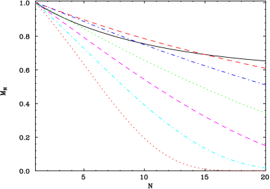
Figure 2: The (normalized) moments $M_{N}$ of the photon spectrum as a function of $N$, as computed through Eq. (10), where $C_{N}(\alpha_{s}(m^{2}))$ is given by Eq. (2.1.4). The full line is the principal–value Borel sum. Dashed, dotdash and dotted lines correspond to truncation of the Sudakov exponent at increasing logarithmic accuracy – the uppermost line is LL, then NLL, etc.

While at low moments the principal–value regularization is numerically close to NNLL truncation, at higher $N$ it approaches NLL and then LL, and finally crosses even the LL result developing milder slope at high $N$. This behaviour is in one–to–one correspondence with the fact that as $N$ increases, the perturbative expansion for the exponent breaks down earlier. It should be emphasized that when the exponent is written at fixed logarithmic accuracy (NLL and beyond) it suffers from Landau singularities. This is not the case for the principal–value Borel sum [48] which extrapolates smoothly to high–$N$ values.

Note that the NNLL and further subleading logarithms are not computed exactly but are only estimated based on the expansion of Eq. (10). Nevertheless, we expect that the corresponding curves in Fig. 2 represent well the divergence of the perturbative expansion. As usual in asymptotic expansions there is no use in summing up the series beyond the point where it starts diverging, which is roughly the order that reproduces the principal–value result. Since this never occurs beyond NNLL an exact calculation of subleading logarithms (yet unavailable) is less important for phenomenology in this case than careful treatment of power corrections. What is expected to make a significant impact on phenomenology is the use of power–like separation as provided by the principal–value prescription instead of the commonly used NLL truncation of the Sudakov exponent. As Fig. 2 shows, NLL truncation cannot be considered a good approximation to the principal–value prescription over the entire $N$ range nor does it differ from it by power terms.

2.2 Power corrections

2.2.1 The shape function

As announced, we focus here on the end–point region, namely the large–$N$ limit. The leading non-perturbative corrections in this limit are associated with the soft scale, $m/N$. Through the renormalon calculation we have provided evidence for power corrections on the soft scale, but we have not proven that these are indeed the leading corrections at large $N$. In fact, they are. For example, there are no corrections that scale like $N^{2}\Lambda/m$. A completely general argument will be provided below.

As reflected in the renormalon ambiguity of $S_{N}(m^{2},\mu^{2})$ in Eq. (2.1.3), the leading power correction is ${\cal O}(N\Lambda/m)$, which is potentially very large. It is therefore of primary interest to understand the origin of this correction. This is the main goal of this section. Subleading corrections on the soft scale are important as well and need to be resummed into a shape function [11, 14], as we discuss below. On the other hand, we shall not be interested here in further subleading power corrections ${\cal O}(N\Lambda^{2}/m^{2})$ or ${\cal O}(\Lambda/m)$ which are associated with the jet function and the hard function, respectively.

To include power corrections on the soft scale we replace $S_{N}(m^{2};\mu^{2})$ in our expression for the moments, Eq. (13), by the corresponding matrix–element definition, $\tilde{F}(N;\mu^{2})$. Let $B(p_{B})$ be a meson with momentum $p_{B}$. We define $F(z;\mu^{2})$ as the Fourier transform of the forward hadronic matrix element of two heavy–quarks fields on the lightcone ($y^{2}=0$):

$$F(z;\mu^{2})=\frac{1}{4\pi}\int_{-\infty}^{\infty}\frac{d(p_{B}y)}{p_{B}y}\,{\rm e}^{izp_{B}y}\left<B(p_{B})\left|\bar{\Psi}(0)\mbox{$y$\raisebox{0.43057pt}{$/$}}\Psi(y)\right|B(p_{B})\right>_{\mu^{2}},$$ (23)

and then take moments:

$$\tilde{F}(N;\mu^{2})=\int_{0}^{1}dz\,F(z;\mu^{2})\,z^{N-1}.$$ (24)

Note that $S_{N}(m^{2};\mu^{2})$ of Eq. (2.1.3) is nothing else but the perturbative analogue of $F(z;\mu^{2})$ which is obtained by replacing the hadron by an on–shell heavy quark ($p^{2}=m^{2}$) $q(p)$:

$$F_{\hbox{\tiny PT}}(z;\mu^{2})=\frac{1}{4\pi}\int_{-\infty}^{\infty}\frac{d(py)}{py}\,{\rm e}^{izpy}\left<q(p)\left|\bar{\Psi}(0)\mbox{$y$\raisebox{0.43057pt}{$/$}}\Psi(y)\right|q(p)\right>_{\mu^{2}}.$$ (25)

In moment space $\mu^{2}$ evolution is multiplicative. Since the evolution factors of $\tilde{F}(N;\mu^{2})$ and $\tilde{F}_{\hbox{\tiny PT}}(N;\mu^{2})$ are the same, the ratio

$$\tilde{F}_{\hbox{\tiny NP}}(N)\equiv\frac{\tilde{F}(N;\mu^{2})}{\tilde{F}_{\hbox{\tiny PT}}(N;\mu^{2})}$$ (26)

does not depend on $\mu^{2}$. This function incorporates power corrections on the soft scale $m/N$ which distinguish the heavy meson state from an on-shell heavy quark. We conclude that the non-perturbative formula for the moments takes the form

$$M_{N}=C_{N}(\alpha_{s}(m^{2}))\,S_{N}(m^{2};\mu^{2})\,\tilde{F}_{\hbox{\tiny NP}}(N)\,J_{N}(m^{2};\mu^{2})=M_{N}^{\hbox{\tiny PT}}\,\tilde{F}_{\hbox{\tiny NP}}(N),$$ (27)

The properties of $\tilde{F}_{\hbox{\tiny NP}}(N)$ will be discussed in the following section.

2.2.2 HQET and the OPE

The HQET (see e.g. [51, 52]) is a systematic way to identify the leading contributions to QCD matrix elements in the large mass limit. Here we would like to use this framework to parametrize the shape function $F_{\hbox{\tiny NP}}(z)$ and, in particular, to understand its dependence on the mass definition. We recall that in the perturbative treatment we assumed that the decaying b quark was on-shell. Our answer for the moments of the photon–energy spectrum, Eq. (10), contains an infrared renormalon at $u=1/2$, namely an ${\cal O}(N\Lambda/m)$ ambiguity, which exponentiates together with the perturbative logs. In order to trace the cancellation of this ambiguity in the next section we first need to understand the dependence of $F_{\hbox{\tiny NP}}(z)$ on the definition of the mass.

In the large mass limit the momentum of the heavy quark within the hadron is naturally written as $p=mv+k$ where $v$ is the hadron four velocity, $v\equiv p_{B}/M$, and $k$ is the residual momentum which is small compared to heavy–quark mass $m$. The effective Lagrangian describing the dynamics in the large–$m$ limit is

$${\cal L}_{\hbox{\tiny eff}}=h_{v}(x)(iv\cdot D-\delta m)h_{v}(x)+\cdots,$$ (28)

where $h_{v}(x)$ is the velocity–dependent rescaled quark field,

$$h_{v}(x)={\rm e}^{im_{Q}v\cdot x}\,\frac{1+\mbox{$v$\raisebox{0.43057pt}{$/$}}}{2}\,\Psi(x),$$ (29)

$\delta m\equiv m-m_{Q}$ is the residual mass term which is constant in the large–$m$ limit, $m$ is the pole mass and the dots stand for ${\cal O}(\Lambda/m)$ terms.

The residual mass term [53] appears in the Lagrangian because there is freedom in the choice of the mass $m_{Q}$ in Eq. (29). The natural candidate for $m_{Q}$ is the pole mass ($m$). However, if one is concerned with power terms then specifying $m_{Q}$ as the pole mass does not justify eliminating $\delta m$ in Eq. (28) because the pole mass itself (i.e. its relation with any short–distance mass) has an infrared renormalon at $u=1/2$ [55] which implies that it has an inherent linear ambiguity of order $\Lambda$. This ambiguity is understood on physical grounds: owing to confinement the full quark propagator does not have a pole. Using the pole mass in Eq. (29) would therefore render $\delta m$ zero to any order in the coupling while non-zero and ambiguous as far as power suppressed terms ${\cal O}(\Lambda/m)\sim\exp\left\{-\pi/(2\alpha_{s}(m^{2})\beta_{0})\right\}$ are concerned. It was shown in [55, 57] that upon including an ambiguous $\delta m$ term in the HQET Lagrangian one can trace the dependence of matrix elements on the mass definition and that eventually such ambiguities cancel out in physical observables. It is important to stress that this cancellation does not occur within the HQET but in full QCD, and only provided that the $u=1/2$ infrared renormalon in the coefficient functions relating HQET matrix elements to physical observables are taken into account.

Let us now address the non-perturbative contribution to the b–quark distribution in the B meson, $F_{\hbox{\tiny NP}}(z)$, by considering the matrix–element definition within the HQET. In this framework $\mu^{2}$ is the scale at which the effective theory is matched to the full theory, $\Lambda^{2}\ll\mu^{2}\ll m^{2}$. Since we are not concerned at this point with perturbative corrections we can simply identify $F_{\hbox{\tiny NP}}(z)$ with the matrix–element definition in Eq. (23) taken at Born level. Thus, in the HQET we obtain

$$F_{\hbox{\tiny NP}}(z)=\int_{-\infty}^{\infty}\frac{d(v\cdot y)}{4\pi}\,{\rm e}^{iM(v\cdot y)\left(z-\frac{m_{Q}}{M}\right)}\left<B(Mv)\left|\bar{h}_{v}(0)\,P{\rm e}^{-i\int_{0}^{1}dsy_{-}A_{+}(sy)}\,h_{v}(y)\right|B(Mv)\right>,$$

where we used Eq. (29) and substituted $p_{B}=Mv$. We also wrote explicitly the path–ordered exponential making the matrix element gauge invariant. Note that the normalization of the states in Eq. (2.2.2) is

$$\left<B(Mv)\left|\bar{h}_{v}(0)h_{v}(0)\right|B(Mv)\right>=2M.$$

Next we would like to expand the non-local lightcone operator in Eq. (2.2.2) in terms of local operators. The matrix elements of these operators can be expressed by the parameters of the HQET. A similar expansion was performed in the past, see e.g. [49, 12, 13]. At difference with previous literature, however, we do not put $\delta m$ to zero because we want to distinguish between matrix elements that depend on $\delta m$ and these that do not. The expansion yields:

$$\frac{1}{2M}{\left<B(Mv)\left|\bar{h}_{v}(0)\,P{\rm e}^{-i\int_{0}^{1}dsy_{-}A_{+}(sy)}\,h_{v}(y)\right|B(Mv)\right>}=1+\sum_{k=1}^{\infty}\frac{a_{k}}{k!}\,(-iv\cdot y)^{k},$$ (31)

where

$$(v_{+})^{k}\,a_{k}\equiv\frac{1}{2M}{\left<B(Mv)\left|\bar{h}_{v}(0)(iD_{+})^{k}\,h_{v}(0)\right|B(Mv)\right>}.$$ (32)

The matrix elements $a_{k}$ depend on $\delta m$, which is a parameter of the effective Lagrangian of Eq. (28). Since $\delta m$ represents the ambiguity that should cancel against the $u=1/2$ renormalon in the perturbative coefficient function we would like to isolate this dependence.

Using the equation of motion

$$i(v\cdot D)h_{v}(x)=\delta mh_{v}(x)$$

we can immediately fix the first parameter in Eq. (31), $a_{1}=\delta m$. Using further the matrix element corresponding to the kinetic energy of the b quark inside the meson (see e.g. [12, 11]) we can fix also the second coefficient $a_{2}$. Let us define

$$\frac{1}{2M}{\left<B(Mv)\left|\bar{h}_{v}(0)(g_{\mu\nu}-v_{\mu}v_{\nu})iD^{\mu}iD^{\nu}\,h_{v}(0)\right|B(Mv)\right>}=\lambda_{1}.$$ (33)

As discussed in [11] $\lambda_{1}<0$. It is straightforward to check by a change of variables in the functional integral,

$$\delta m \longrightarrow \widetilde{\delta m},$$

$$h(y) \longrightarrow \widetilde{h}(y)={\rm e}^{i(\widetilde{\delta m}-\delta m)\,vy}\,h(y),$$ (34)

that, like the Lagrangian, $\lambda_{1}$ is independent of $\delta m$. Having established this we express $a_{2}$ in terms of $\lambda_{1}$ exposing explicitly the dependence on $\delta m$: $a_{2}=(\delta m)^{2}-\lambda_{1}/3$. Similarly, to deal with $a_{3}$ we use the definition

$$\frac{1}{2M}{\left<B(Mv)\left|\bar{h}_{v}(0)v_{\nu}D_{\mu}F^{\mu\nu}\,h_{v}(0)\right|B(Mv)\right>} = -3f_{3}.$$ (35)

Also $f_{3}$ is independent of $\delta m$. We can now express the third coefficient as $a_{3}=(\delta m)^{3}-\lambda_{1}\delta m+f_{3}$. It is convenient to define $f_{2}\equiv-\lambda_{1}/3>0$ and then the first three coefficients are:

$$a_{1} = \delta m,$$

$$a_{2} = (\delta m)^{2}+f_{2},$$

$$a_{3} = (\delta m)^{3}+3f_{2}\delta m+f_{3}.$$ (36)

This procedure can be continued to higher orders. At each order $n$ the coefficient $a_{n}$ contains at least one new parameter which is unrelated to the definition of the mass and thus enters with $(\delta m)^{0}$; in addition $a_{n}$ contains a polynomial of order $n$ in $\delta m$. We observe, however, that the $\delta m$–dependent terms have a very specific structure (to any order): they exponentiate. The r.h.s. of Eq. (31) can be resummed, getting

$$\frac{1}{2M}{\left<B(Mv)\left|\bar{h}_{v}(0)\,P{\rm e}^{-i\int_{0}^{1}dsy_{-}A_{+}(sy)}\,h_{v}(y)\right|B(Mv)\right>} =$$ (37)

$${\rm e}^{-iv\cdot y\delta m}\,\times\,\left[1+(-iv\cdot y)^{2}\frac{f_{2}}{2}+(-iv\cdot y)^{3}\frac{f_{3}}{6}+\cdots\right] \equiv {\rm e}^{-iv\cdot y\delta m}\,{\cal F}(-iv\cdot y\Lambda),$$

where the sum in the square brackets, and therefore the function ${\cal F}(-iv\cdot y\Lambda)$, are entirely free of the $u=1/2$ renormalon ambiguity; $\Lambda$ appearing in ${\cal F}(-iv\cdot y\Lambda)$ is the QCD scale: it must not be identified with the ambiguous $\bar{\Lambda}=M-m$. The exponential factor in Eq. (37) can be understood from general considerations: it is a reminiscent of the scaling of the fields in Eq. (29). The ambiguity in the mass used to define the HQET reappears as an exponential factor in the parametrization of the matrix element of Eq. (31).

Using Eq. (37), Eq. (2.2.2) becomes

$$F_{\hbox{\tiny NP}}(z)=\int_{-\infty}^{\infty}\frac{d\omega}{2\pi}\,{\rm e}^{i\omega\left(z-\frac{m_{Q}+\delta m}{M}\right)}\,{\cal F}(-i\omega\Lambda/M)+{\cal O}(\Lambda/M),$$ (38)

exhibiting the fact [53] that the residual mass term $\delta m$ enters matrix elements only in the combination $m_{Q}+\delta m=m$.

Next, using Eq. (38) together with the definition of the moments, Eq. (24), one can show that to leading order in $1/N$,

$$\tilde{F}_{\hbox{\tiny NP}}(N) = {\rm e}^{-(N-1)\bar{\Lambda}/M}\,{\cal F}((N-1)\Lambda/M)+{\cal O}(\Lambda/M)$$

$$= {\rm e}^{-(N-1)\bar{\Lambda}/M}\,\bigg{[}1+\frac{f_{2}}{2!}\left(\frac{(N-1)\Lambda}{M}\right)^{2}+\frac{f_{3}}{3!}\left(\frac{(N-1)\Lambda}{M}\right)^{3}\,+\,\cdots\bigg{]}\,+{\cal O}(\Lambda/M),$$

where we used the definition $\bar{\Lambda}=M-m=M-m_{Q}-\delta m$ in the exponential factor. To derive this relation one first converts the Mellin integral over $z$ into Laplace, neglecting ${\cal O}(1/N)$ (or, equivalently, ${\cal O}(\Lambda/M)$) corrections. The $z$ integral is then straightforward. Finally, the $\omega$ integral can be done by closing a contour in the complex plane picking up the residue at $\omega=i(N-1)$. In the following, as in Eq. (2.2.2), we shall explicitly use $m$ (and $\bar{\Lambda}$) rather than $m_{Q}$. The reader should keep in mind that this parameter is ambiguous.

Note that Eq. (2.2.2) is scaling law. For example, it excludes corrections scaling like ${\cal O}(N^{2}\Lambda/M)$. Put differently, it implies that there is one natural way to take the large $N$ and large $M$ limits, namely with the ratio $N\Lambda/M$ fixed.

Note also that in Eq. (2.2.2) we have chosen to write everywhere $N-1$ rather than $N$ in order to impose the requirement that $\tilde{F}_{\hbox{\tiny NP}}(N=1)=1$ (which is fixed by the overall normalization of the moments, $M_{N=1}\equiv 1$) without involving additional ${\cal O}(1/N)$ terms. This way our approximation for $\tilde{F}_{\hbox{\tiny NP}}(N)$ captures correctly not only the large–$N$ limit but also the $N=1$ limit.

We stress again the distinction between the first factor in Eq. (2.2.2), ${\rm e}^{-(N-1)\bar{\Lambda}/M}$ which contains a mass–related renormalon ambiguity at $u=1/2$ and the second factor, ${\cal F}((N-1)\Lambda/M)$, which is free of this ambiguity. ${\cal F}((N-1)\Lambda/M)$ does not depend on the quark mass but only on the physical meson mass through the ratio $(N-1)\Lambda/M$. Besides this fact, the most important property of this function is that its linear term in the small $(N-1)\Lambda/M$ expansion vanishes, as shown in the second line of Eq. (2.2.2).

Having established that ${\cal F}((N-1)\Lambda/M)$ itself is free of any $u=1/2$ renormalon ambiguity, it is important to recall that this function, or alternatively the values of matrix elements $f_{n}$, do contain (in general) other ($u\neq 1/2$) renormalon ambiguities of ultraviolet origin. Similarly to higher–twist corrections to deep inelastic structure functions these matrix elements need to be defined by specifying a regularization prescription for the renormalons which corresponds to the one used for infrared renormalons in the perturbative coefficient function.

At this point it is useful to compare Eq. (2.2.2) with the renormalon–based ansatz of Eq. (12). The leading term, ${\cal O}((N-1)\Lambda/M)$ exponentiates in both. Note, however, that the reasoning that lead us to deduce that exponentiation occurs was completely different: in Eq. (12) it was based on the exponentiation of perturbative soft radiation while in Eq. (12) it was based on the dependence of the heavy–quark field on the mass. Higher–order terms in the HQET analysis do not exponentiate but this cannot be considered as contradiction between the two, as we do not know how to sum the series of power terms. A more significant difference is the presence of a second power ${\cal O}(((N-1)\Lambda/M)^{2})$ in Eq. (2.2.2), associated with the kinetic energy of the heavy quark inside the meson in contrast with its absence in Eq. (12). We recall that the latter is a consequence of the vanishing of the corresponding renormalon residue in the perturbative result, Eq. (10), in the large–$\beta_{0}$ limit. In spite of the vanishing of this renormalon, it is sensible to allow an ${\cal O}(((N-1)\Lambda/M)^{2})$ term in a phenomenological model for power corrections. To understand this term from the renormalon perspective note that: (1) Generally, absence of a renormalon does not imply the vanishing of the corresponding non-perturbative parameter, only the vanishing of its ambiguity. Thus, Eq. (12) should only be considered as a minimal parametrization, not a constraining one. (2) It has been shown in [63] that in the case of the kinetic energy of the b quark a renormalon singularity does appear when going beyond the single–dressed–gluon approximation.

2.2.3 Cancellation of the $u=1/2$ renormalon

It is well known [56, 57] that the total semi-leptonic decay width,

$$\Gamma(\bar{B}\longrightarrow X_{u}l\bar{\nu})=\frac{G_{F}^{2}\left|V_{ub}\right|^{2}m^{5}}{192\pi^{3}}\left[1-\frac{2\alpha_{s}(m^{2})}{3\pi}\left(\pi^{2}-\frac{25}{4}\right)+\cdots\right],$$ (40)

is free of any $u=1/2$ renormalon ambiguity. If the pole mass is used in the calculation an intricate cancellation occurs between the $u=1/2$ ambiguity contained in the overall factor $m^{5}$ and that associated with the sum of the perturbative series in the square brackets. If a short–distance mass is used instead, these two factors are separately free of such ambiguities. Here we show that similar cancellation takes place in differential decay spectra.

To demonstrate the cancellation of ambiguities we shall resum the perturbative series in the single–dressed–gluon (large–$\beta_{0}$) approximation. One difference with respect to the total width is that when considering the spectrum we need to take into account exponentiation: Sudakov exponentiation on the perturbative side and the exponentiation of the $\delta m$ terms on the non-perturbative side.

Let us first consider the ambiguity in the non-perturbative function in Eq. (2.2.2) in this approximation. The result is:

$$\tilde{F}_{\hbox{\tiny NP}}(N) \simeq {\rm e}^{-(N-1)({M-m})/{M}}\,{\cal F}((N-1)\Lambda/M)$$

$$= {\rm e}^{(N-1)\Delta m/M}\,\times\,{\rm e}^{-(N-1)(M-m_{\hbox{\tiny PV}})/M}{\cal F}((N-1)\Lambda/M)$$

with

$$\frac{\Delta m}{m}\equiv\frac{m-m_{\hbox{\tiny PV}}}{m}\simeq\frac{C_{F}}{2\beta_{0}}\left[\int_{0}^{\infty}du\,T(u)\left(\frac{\Lambda^{2}}{m^{2}}\right)^{u}\,\frac{{\rm e}^{cu}}{\frac{1}{2}-u}\,-\,{\rm PV}\int_{0}^{\infty}du\,T(u)\left(\frac{\Lambda^{2}}{m^{2}}\right)^{u}\,\frac{{\rm e}^{cu}}{\frac{1}{2}-u}\right],$$ (42)

where, as before, we define $\Lambda$ in ${\overline{\rm MS}}$ so $c=5/3$. Here $m_{\hbox{\tiny PV}}$ stands for the pole mass in which the $u=1/2$ renormalon is regularized by the principal–value prescription. Eq. (42) is correct to leading order in $1/\beta_{0}$; we also neglected higher power corrections ${\cal O}(\Lambda^{3}/m^{3})$. The explicit expression for $\frac{\Delta m}{m}$ in the large–$\beta_{0}$ limit was obtained based on the known relation [56, 55, 57] in this limit between the pole mass and short–distance mass definitions. In particular the relation with the ${\overline{\rm MS}}$ mass is

$${\frac{m-m_{\hbox{\tiny${\overline{\rm MS}}$}}}{m}}=\frac{C_{F}}{2\beta_{0}}\int_{0}^{\infty}du\,T(u)\left(\frac{\Lambda^{2}}{m}\right)^{u}\,\left[{\rm e}^{cu}\frac{3(1-u)\Gamma(u)\Gamma(1-2u)}{\Gamma(3-u)}+\frac{1}{2u}\,\widetilde{G}(u)\right],$$ (43)

where $\widetilde{G}(u)$ depends on the ${\overline{\rm MS}}$ counter terms for the mass and it is free of renormalons. Note that since the difference between masses is ${\cal O}(1/\beta_{0})$ it does not matter (to leading order in $1/\beta_{0}$) which mass is used to normalize the mass difference in the equations above.

Let us turn now to the perturbative side. We recall that owing to the integration over $x$ near $1$, the perturbative moments $M_{N}^{\hbox{\tiny PT}}$ of Eq. (10) have a renormalon ambiguity at $u=1/2$ which is associated with the soft scale $m/N$. Using in Eq. (10) the principal–value prescription to define $\left.M_{N}^{\hbox{\tiny PT}}\right|_{\hbox{\tiny PV}}$ we obtain:

$$M_{N}^{\hbox{\tiny PT}}\simeq\left.M_{N}^{\hbox{\tiny PT}}\right|_{\hbox{\tiny PV}}\,\times\,\exp\Bigg{\{}\frac{C_{F}}{2\beta_{0}}\bigg{[} \!\!\!\!\int_{0}^{\infty}du\,T(u)\,\left(\frac{\Lambda^{2}}{m^{2}}\right)^{u}\,\frac{{\rm e}^{cu}}{\frac{1}{2}-u}\left(N^{2u}-1\right)\big{(}1_{\rm I}-2_{\rm II}+0_{\rm III}\big{)}$$

$$-{\rm PV} \!\!\!\!\int_{0}^{\infty}du\,T(u)\,\left(\frac{\Lambda^{2}}{m^{2}}\right)^{u}\,\frac{{\rm e}^{cu}}{\frac{1}{2}-u}\left(N^{2u}-1\right)\big{(}1_{\rm I}-2_{\rm II}+0_{\rm III}\big{)}\bigg{]}\Bigg{\}},$$

where the subscripts I, II and III indicate the diagram in Fig. 1 from which each contribution originates in the Feynman gauge, cf. Eq. (2.1.1). Note that in Eq. (2.2.3) we have isolated the $u=1/2$ pole ignoring subleading power corrections which are unrelated to this renormalon. We stress that although the large–$N$ limit has been taken to arrive at Eq. (10), our result for the $u=1/2$ residue (in the large–$\beta_{0}$ limit) as expressed by Eq. (2.2.3) is exact: as one can verify by taking moments of the exact expression in $x$ space, Eq. (2.1.1), there are no subleading $1/N$ corrections which have renormalon ambiguities at $u=1/2$. The reason is that this renormalon is directly related to the integration over $x$ in the singular $x=1$ limit.

Finally, substituting in Eq. (27) the perturbative and non-perturbative factors of Eq. (2.2.3) and Eq. (2.2.3), respectively, we get

$$M_{N}=M_{N}^{\hbox{\tiny PT}}\tilde{F}_{\hbox{\tiny NP}}(N)=\left.M_{N}^{\hbox{\tiny PT}}\right|_{\hbox{\tiny PV}}\,{\rm e}^{-(N-1)(M-m_{\hbox{\tiny PV}})/M}{\cal F}((N-1)\Lambda/M),$$ (45)

where the ambiguous exponential factors cancel out in the product. The result is entirely free of the $u=1/2$ renormalon ambiguity. Moreover, it is independent of the regularization prescription for the $u=1/2$ renormalon pole; what is important is that the same prescription (here principal value of the Borel sum) is used on both the perturbative Sudakov exponent in $\left.M_{N}^{\hbox{\tiny PT}}\right|_{\hbox{\tiny PV}}$ and on the pole mass in ${\rm e}^{-(N-1)(M-m_{\hbox{\tiny PV}})/M}$. Let us stress that Eq. (45) resums only power corrections depending on the soft scale, $M/N$: subleading power corrections such as ${\cal O}(\Lambda/M)$ or ${\cal O}(\Lambda^{2}N/M^{2})$ are neglected here.

The implications of Eq. (45) become more intuitive upon returning to $x$ space. Using the inverse Mellin transform we have

$$\frac{1}{\Gamma_{\hbox{\tiny total}}}\frac{d\Gamma(x)}{dx} = \frac{1}{2\pi i}\int_{\cal C}dN\,x^{-N}M_{N}$$ (46)

$$\simeq \frac{1}{2\pi i}\int_{\cal C}dN\,{\rm e}^{(N-1)\left(1-x-\frac{M-m_{\hbox{\tiny PV}}}{M}\right)}\,\left.M_{N}^{\hbox{\tiny PT}}\right|_{\hbox{\tiny PV}}\,{\cal F}((N-1)\Lambda/M),$$

where in the second line we neglected ${\cal O}(1/N)$ terms. If we neglect the effect of ${\cal F}((N-1)\Lambda/M)$ in Eq. (46) altogether, the only effect of confinement is to shift the perturbative spectrum in $x$ by the energy fraction of the light degrees of freedom in the meson, $(M-m)/M$, away from the endpoint, towards smaller values of $x$:

$$\frac{1}{\Gamma_{\hbox{\tiny total}}}\frac{d\Gamma(x)}{dx}\sim\frac{1}{\Gamma_{\hbox{\tiny total}}}\frac{d\Gamma^{\hbox{\tiny PT}}_{\hbox{\tiny PV}}(x+\frac{M-m_{\hbox{\tiny PV}}}{M})}{dx}.$$ (47)

Note that the shifted spectrum does not depend anymore on the quark mass definition or on the fact that the principal–value prescription was used (for both the Sudakov exponent and the pole mass). The finding that the leading effect of confinement is a shift of the perturbative spectrum is not surprising nor unique to $B$ physics. It is a general feature of differential cross sections near kinematic thresholds. For example, a shift occurs in event–shape distributions which peak near the two jet limit [64, 65, 41]. What is special though is that in the $B$–decay case one can fix the magnitude of the shift in terms of a familiar non-perturbative parameter.

It should be stressed that this shift has nothing to do with the fact that the physical endpoint is at $E_{\gamma}=M/2$ whereas the perturbative one is at $E_{\gamma}=m/2$; note that Eq. (47) concerns the spectrum in the dimensionless scaling variable $x$. In fact, when addressing the close vicinity of endpoint the function ${\cal F}((N-1)\Lambda/M)$ cannot be neglected in Eq. (46). Physically, ${d\Gamma(x)}/{dx}$ has support for $0<x<1$. The perturbative spectrum which is calculated using the principal–value prescription in moment space does not respect the physical support properties and these should be recovered in Eq. (46) when the shift generated by the exponential as well as the additional smearing generated by the subleading power corrections in ${\cal F}((N-1)\Lambda/M)$ are taken into account. If $(N-1)\Lambda/M$ is not too large the leading power correction in ${\cal F}((N-1)\Lambda/M)$ is that of the kinetic energy of the $b$ quark inside the meson, $f_{2}$. However, near the endpoint higher power terms become as important.

The reader should also keep in mind that the spectrum computed by Eq. (46) is a priori just a rough description of the physical one at $x$ values away from the endpoint region: there are additional ${\cal O}(1/N)$, or ${\cal O}(\Lambda/M)$, effects which were neglected altogether. Formally, our analysis (perturbative and non-perturbative) applies only at large $N$. Having fixed, in addition to the large–$N$ limit, the $N=1$ moment one can hope that the numerically most important corrections in the first few moments are accounted for, but this is not guaranteed and it will be eventually decided by the data. Experience in other applications [41, 48] is very encouraging in this respect.

3 Semi-leptonic decay

In this section we consider the semi-leptonic decay $\bar{B}\longrightarrow X_{u}l^{-}\bar{\nu}_{l}$ and perform a DGE calculation in analogy with the radiative decay presented above. Let us start by describing the kinematics. We call the $b$–quark momentum $p$, and the momentum of the leptons $k_{\bar{\nu}_{l}}$ and $k_{l}$. Let us also denote the total momentum of the lepton system by $q\equiv k_{\bar{\nu}_{l}}+k_{l}$. We will express the distribution in terms of $x\equiv 2pk_{l}/m^{2}$, $y\equiv 2pq/m^{2}$ and the leptonic invariant mass fraction $z\equiv q^{2}/m^{2}$. In the $B$ rest frame $y$ has the meaning of the total leptonic energy ($E$) fraction, $y=2E/m$, while $x$ is the electron (or muon) energy fraction. The hadronic system (a $u$–quark jet) has momentum $l$ and invariant mass

$$l^{2}=q^{2}+m^{2}(1-y)=m^{2}(1-y+z).$$ (48)

The semi-leptonic decay rate is given by

$$\Gamma=\frac{G_{F}^{2}|v_{ub}|^{2}}{2m}\,\int d{\rm LIPS}(p\longrightarrow k_{\bar{\nu}_{l}}+k_{l}+l)\,\,{\rm Im}\left\{L^{\mu\nu}T_{\mu\nu}\right\}.$$ (49)

Writing the phase–space integral in terms of $x$, $y$ and $z$ we have:

$$\!\!\Gamma\!=\!\frac{G_{F}^{2}|v_{ub}|^{2}\,m^{3}}{64\pi^{4}}\,\int_{0}^{1}\!dz\,\int_{z}^{1}dx\int_{x+\frac{z}{x}}^{1+z}\!\!dy\,{\rm Im}\left\{A_{\rm Born}+\frac{C_{F}\alpha_{s}}{4\pi}\left[A_{\rm I}+2A_{\rm II}+A_{\rm III}\right]\right\},$$ (50)

where $A_{\rm Born}$ stands for the Born diagram contracted with the leptonic tensor, and $A_{\rm I,II,III}$ correspond to the three one–loop diagrams in the Feynman gauge, contracted with the leptonic tensor. The Born level result is: $A_{\rm Born}=-{\displaystyle{4\,m^{4}\,(x-z)\,(y-x)}/{{l^{2}}}}$. Taking the imaginary part we get

$${\rm Im}\left\{A_{\rm Born}\right\} = 4m^{2}(x-z)\,(y-x)\times\pi\delta(1-y+z).$$ (51)

Next, we compute the one–loop diagrams with a dressed gluon. The calculation is more complicated than that of the radiative decay owing to the presence of additional kinematic variables. In Appendix B.1 we summarize the full result as a double Feynman parameter integral. The interest here, however, is in the specific kinematic limit where Sudakov logs appear: based on the Born–level calculation this limit is $y\longrightarrow 1+z$.

We observe that the phase–space structure of Eq. (50) implies that the region $y\simeq 1+z$ becomes relevant for $x\longrightarrow 1$: the lower limit in the integration over $y$ approaches $1+z$, which is also the upper limit. Thus, if one considers the spectrum near the endpoint $x\longrightarrow 1$ the Sudakov region is indirectly selected. Nevertheless, one can approach the Sudakov limit differently, e.g. by considering directly the region where the hadronic system has small invariant mass. Below we first present a triple differential spectrum to leading power in $(1+z-y)$ allowing one to approach the Sudakov limit in different ways. Then we focus on the specific example of the single differential rate in $x$ to leading power in $(1-x)$.

In Appendix B.2 we compute all the singular terms of the semi-leptonic decay in the limit $y\longrightarrow 1+z$ in the single–dressed–gluon approximation. Combining the jet and soft functions, Eq. (B.2.1) and Eq. (83), respectively, and using Eq. (50) we arrive at the following triple differential decay rate to leading power in $(1+z-y)$:

$$\frac{1}{\Gamma_{\hbox{\tiny total}}}\frac{d\Gamma(y,x,z)}{dydxdz}=12\,(x-z)(1+z-x)\,\left\{\delta(1+z-y)+\frac{C_{F}}{2\beta_{0}}\int_{0}^{\infty}du\,T(u)\left(\frac{\Lambda^{2}}{m^{2}}\right)^{u}{\rm e}^{cu}\right.$$

$$\left.\,\,\times\left[\frac{2}{u}\frac{1-u}{1-z}\Big{(}\frac{1+z-y}{1-z}\Big{)}^{-1-2u}-\left(\frac{2}{u}+\frac{1}{1-u}+\frac{1}{2-u}\right)\frac{\sin\pi u}{\pi u}\Big{(}1+z-y\Big{)}^{-1-u}\right]\right\},$$ (52)

where we normalized the spectrum dividing by the total decay width:

$$\Gamma_{\hbox{\tiny total}}=\Gamma_{0}\times(1+{\cal O}(\alpha_{s})),\quad\quad\Gamma_{0}=\frac{G_{F}^{2}|v_{ub}|^{2}m^{5}}{192\pi^{3}},$$ (53)

where $\Gamma_{0}$ is the Born–level width. Eq. (3) is the analogue of Eq. (2.1.2).

We note that the general $u$-dependent structure of the soft and the jet functions in Eq. (83) and Eq. (B.2.1) is the same as in the radiative decay (cf. Eq. (2.1.2)), the difference being restricted to the $z$ dependence of the two scales involved. Here the soft function depends on $m(1+z-y)/(1-z)$ and the jet function on $m^{2}(1+z-y)$. Clearly, in the limit $z\longrightarrow 0$ Eq. (3) reduces to Eq. (2.1.2), where $y$ in the former takes the role of $x$ in the latter.

We recall that these functions appear not only in heavy–flavor decay spectra, but also in other differential cross sections near a kinematic threshold. The perturbative soft function is associated with radiation off a heavy quark close to its mass shell, and it therefore describes also the heavy–quark fragmentation function [48]. The jet function [28, 29, 30, 31, 32, 33, 34, 35] occurs even more frequently: it is not specific to heavy–quark physics. It describes radiation off an unresolved jet with a constrained invariant mass $l^{2}$. In the framework of DGE the same expression for the jet function has already been obtained in the context of deep inelastic structure functions at large Bjorken $x$ [45, 46, 47], single–particle inclusive cross sections in $e^{+}e^{-}$ annihilation for light [45] and heavy quarks [48] and event–shape distributions [41, 44].

Infrared and collinear safety requires cancellation of $u=0$ poles between the soft and the jet functions. Indeed, the result is finite: the expansion of the Borel function in the square brackets of Eq. (3) is

$$\frac{-1}{1+z-y}\left(2\ln(1+z-y)-4\ln(1-z)+\frac{7}{2}\right)+{\cal O}(u).$$ (54)

This (times $C_{F}/(2\pi)$) is the logarithmically–enhanced part of the coefficient of $\alpha_{s}$ in the perturbative expansion. One immediately identifies the double– and the single–logarithmic terms of $(1+z-y)$. At difference with the radiative–decay case, there are also single logs of $(1-z)$ originating from the soft function, which mix with those of $(1+z-y)$. Note that $z\longrightarrow 1$ corresponds to another singular limit (not considered here) where the invariant mass of the lepton pair approaches the total b–quark mass.

To resum soft–gluon radiation, Eq. (3) needs to be exponentiated in moment space in analogy with Eq. (10). Natural moment–space definitions are with respect to $y-z$, or the electron energy fraction $x$. In the following we concentrate on the latter possibility, which is useful for describing the single differential rate with respect to $x$. To this end we need to integrate the triple differential rate, Eq. (3), over the phase space: for any fixed $x$ ($0\leq x\leq 1$) the available phase space (cf. Eq. (50)) is

$$\int_{0}^{x}dz\int_{x+\frac{z}{x}}^{1+z}dy\, = \,\int_{1}^{1+x}dy\int_{y-1}^{x(y-x)}dz+\int_{x}^{1}dy\int_{0}^{x(y-x)}dz$$ (55)

$$\simeq \int_{1}^{1+x}dy(2-y)\int_{\frac{1+x^{2}-xy}{2-y}}^{1}d\xi\simeq\int_{1}^{2}dy(2-y)\int_{x}^{1}d\xi,$$

where in the first step we changed the order of integration keeping the exact phase space; in the second we neglected the second term which is ${\cal O}(1-x)$ with respect to the first; in the third we changed variables to $\xi\equiv({1-z})/({2-y})$; and in the fourth approximated the integration limits neglecting ${\cal O}(1-x)$ terms.

Integrating the single–dressed–gluon result, Eq. (3), over this approximate phase space we retain exactly the leading power in $(1-x)$. In order to preform exponentiation we now take moments with respect to $x$,

$$M_{N}^{\rm sl}=\int_{0}^{1}dx\,x^{N-1}\,\int_{1}^{2}dy(2-y)\int_{x}^{1}d\xi\,\,\frac{1}{\Gamma_{\hbox{\tiny total}}}\left.\frac{d\Gamma(y,x,z)}{dydxdz}\right|_{z=1-\xi(2-y)}.$$ (56)

Using Eq. (3), the DGE formula takes the form:

$$M_{N}^{\rm sl}=C_{N}^{\rm sl}(\alpha_{s}(m^{2}))\,\exp\bigg{\{}\frac{C_{F}}{2\beta_{0}}\int_{0}^{\infty}du\,T(u)\,\left(\frac{\Lambda^{2}}{m^{2}}\right)^{u}\,{\rm e}^{cu}\,\bigg{[}\frac{2}{u}(1-u)\,\Gamma(-2u)\left(N^{2u}-1\right)$$

$$\hskip 30.0pt-\left(\frac{2}{u}+\frac{1}{1-u}+\frac{1}{2-u}\right)\frac{6}{(2-u)(3-u)}\,\frac{\sin\pi u}{\pi u}\,\Gamma(-u)\left(N^{u}-1\right)\bigg{]}\bigg{\}},$$ (57)

where we absorbed an overall factor ($\sim 2/N$ at large $N$) into the coefficient $C_{N}^{\rm sl}$ and exponentiated the logarithmic terms. There are two differences with respect to the radiative decay case, Eq. (10). The most important one that here $C_{N}^{\rm sl}$ is ${\cal O}(1/N)$ rather than ${\cal O}(1)$. The other is the factor ${6}/[{(2-u)(3-u)}]$ in the second term which emerges from a weighted integral over the jet function, the integral over $y$ in Eq. (56).

Upon expanding the exponential and the Borel sum to order $\alpha_{s}$ we obtain:

$$M_{N}^{\rm sl}=C_{N}^{\rm sl}(\alpha_{s}(m^{2}))\left\{1+\frac{C_{F}\alpha_{s}}{2\pi}\left[-\ln^{2}N+\left(\frac{31}{6}-2\gamma_{E}\right)\ln N\right]+{\cal O}(\alpha_{s}^{2})\right\}.$$ (58)

Note that the constant ($N$–independent) terms are all in $C_{N}^{\rm sl}(\alpha_{s}(m^{2}))$. This result for the leading and next–to–leading logarithmic terms agrees with the known ${\cal O}(\alpha_{s})$ coefficient, see [2, 19].

It is now straightforward to match our resummed spectrum, Eq. (3), to the exact ${\cal O}(\alpha_{s})$ result to account for subleading powers of $1/N$. The matching coefficient function is given by:

$$C_{N}^{\rm sl}(\alpha_{s}(m^{2}))\,=\,\frac{2\,(N+5)}{(N+2)\,(N+3)}\,\times\Bigg{\{}1+\frac{C_{F}\alpha_{s}}{2\pi}\bigg{\{}\bigg{[}-\left(\Psi(N)+\gamma_{E}\right)^{2}+\Psi_{1}(N)-{\frac{\pi^{2}}{6}}$$

$$+\left(-{\frac{5}{N+1}}+{\frac{31}{6}}-{\frac{6}{5\,(N+5)}}+{\displaystyle\frac{31}{5\,N}}\right)\,\left(\Psi(N)+\gamma_{E}\right)+{\frac{11}{3\,(N+2)}}-{\frac{11}{150\,N}}$$

$$\mbox{}-{\frac{15}{2}}+{\frac{211}{150\,(N+5)}}-{\frac{5}{(N+1)^{2}}}+{\frac{4}{3\,(N+3)}}+{\frac{31}{5\,N^{2}}}+{\frac{5}{3\,(N+1)}}\bigg{]}$$

$$-\left[{-\mathrm{ln}^{2}N+\left({\frac{31}{6}-2\,\gamma_{E}}\right)\,\mathrm{ln}N}\right]\bigg{\}}+{\cal O}\left(\alpha_{s}^{2}\right)\Bigg{\}}.$$ (59)

Eq. (3) together with Eq. (3) summarizes our perturbative result for the electron spectrum in the semi-leptonic decay. As usual, the perturbative sum in Eq. (3) needs a prescription for renormalon ambiguities. Once regularized, this spectrum can be combined with non-perturbative corrections and then converted to $x$ space according to Eq. (46). It is natural to use the same regularization prescription as in the radiative decay (the principal value). Only then can we identify the shape function between the two physical processes.

4 Conclusions

We presented here a new approach to describe inclusive B–decay spectra in QCD focusing on the endpoint region, $x\longrightarrow 1$. We observe that precise description of the spectra near the endpoints requires power–like separation between perturbative and non-perturbative contributions on the soft scale, $M/N$. Our approach to the problem is based on Dressed Gluon Exponentiation (DGE) and it differs from conventional Sudakov resummation by running–coupling effects, renormalons, which probe the inherent power–like ambiguity of the Sudakov exponent. The non-perturbative contribution to the b-quark distribution in the meson is, by itself, ambiguous, so it can only be defined in correspondence with the regularization of the renormalons in the perturbative result. For the leading renormalon, ${\cal O}(N\Lambda/M)$, we have explicitly shown how a regularization–prescription (or mass–scheme) independent, well-defined answer emerges owing to cancellation of ambiguities between the Sudakov exponent and the definition of the pole mass. At the end the effect of the leading power correction, ${\rm e}^{-(N-1)\bar{\Lambda}/M}$ in Eq. (2.2.2), is to shift the perturbative spectrum in $x$ by the relative mass difference between the meson and the quark. This result is important for phenomenology, as it opens up the possibility to fix the leading non-perturbative correction without using the data.

The DGE perturbative prediction for moments of the photon energy spectrum in the $B\longrightarrow X_{s}\gamma$ decay is summarised by Eq. (10) with the matching coefficient of Eq. (2.1.4). After taking the principal–value Borel integral this result can be readily converted to $x$ space by an inverse Mellin transform. It is important to note that having performed a principal–value sum, the result is free of any Landau singularity (see [48]). This stands in sharp contrast with the standard fixed–logarithmic–accuracy approximation, e.g. [16, 20, 21], which always presents such a singularity at $N\sim{\cal O}(M/\Lambda)$. In practice, it is probably most convenient to include the parametrization of non-perturbative corrections, Eq. (2.2.2), directly in moment space and then convert to $x$ space according to Eq. (46) in order to compare with data.

Let us recall at this point that having concentrated on the specific problems of the endpoint region, we neglected other effects which are important for the phenomenology of radiative decays. One example is running–coupling effects, which have been shown [18] to be important away from the endpoint at order $\alpha_{s}^{2}$. Such corrections can be extracted from Eq. (2) to any order. Other ${\cal O}(\alpha_{s}^{2})$ corrections, which are harder to compute, may eventually be non-negligible. Obviously, one should also consider the contribution of operators other than the magnetic one (Eq. (1)) on both the perturbative and non-perturbative levels. These involve qualitatively different effects. For example, the operator $(\bar{c}_{L\alpha}\gamma^{\mu}b_{L\alpha})(\bar{s}_{L\beta}\gamma_{\mu}c_{L\beta})$ involves a non-perturbative contribution associated with the production of an intermediate $J/\Psi$ state.

The analogous DGE perturbative prediction for the moments of the charged–lepton energy spectrum in the $\bar{B}\longrightarrow X_{u}l^{-}{\bar{\nu}}_{l}$ decay is summarised by Eq. (3) and the matching coefficient of Eq. (3). As previously discussed, non-perturbative corrections corresponding to the b-quark distribution in the B meson are the same as in the $\bar{B}\longrightarrow X_{s}\gamma$ decay. We note that other differential distributions in the $\bar{B}\longrightarrow X_{u}l^{-}{\bar{\nu}}_{l}$ decay, such as the distribution in the invariant mass of the hadronic system near the endpoint, can be readily computed from Eq. (3) by phase–space integration and exponentiation in the appropriate moment space.

On the theoretical side it is interesting to observe the universal structure of the perturbative soft and jet functions. These two functions were shown to be the same for the semi-leptonic decay and the radiative $\bar{B}\longrightarrow X_{s}\gamma$ decay involving the magnetic operator; the difference between the two cases is restricted to the relations between the arguments of the functions and the scaling variables (cf. Eq. (3) and Eq. (2.1.2)). Moreover, this perturbative universality extends beyond the application to B decay. The soft function of Eq. (2.1.3) represents radiation off a heavy quark which is close to its mass shell and thus it also describes the perturbative contribution to heavy–quark fragmentation [48]. The jet function describes radiation off an unresolved jet with a constrained invariant mass and it is particularly important in the analysis of deep inelastic structure function at large Bjorken $x$, where it is the only source of Sudakov logs [45, 46, 47]. It also appears in single–particle inclusive cross sections in $e^{+}e^{-}$ annihilation for light [45] and heavy quarks [48] as well as in event–shape distributions [41, 44].

Appendix A Extracting singular terms in $\bar{B}\longrightarrow X_{s}\gamma$

Here we summarize the formulae used to compute the singular terms in the $x\longrightarrow 1$ limit from the full single–dressed–gluon result of Eq. (2). In order to deal with the Feynman–parameter integrals we use asymptotic expansions of the form:

$$\int_{0}^{1}d\alpha\frac{\alpha}{1-x\alpha}(1-\alpha)^{-u}=\frac{-1}{u(1-u)}\left(1+\frac{{1-x}}{1+u}+{\cal O}\left(({1-x})^{2}\right)\right)+\,\frac{\pi}{\sin\,\pi u}\,(1-x)^{-u}x^{u-2},$$

$$\int_{0}^{1}d\alpha\frac{\alpha^{2}}{(1-x\alpha)^{2}}(1-\alpha)^{-u}=\frac{1}{u(1-u)(1+u)}\left(1+{\cal O}(\left(1-x\right))\right)$$ (60)

$$\hskip 140.0pt+\,\frac{\pi}{\sin\,\pi u}\,(1-x)^{-u-1}x^{u-3}\left(u-2(1-x)\right).$$

The result is:

$$\frac{1}{\Gamma_{\hbox{\tiny total}}}\frac{d\Gamma}{dx} = (1+{\cal O}(\alpha_{s}))\delta(1-x)+\frac{C_{F}}{2\beta_{0}}\int_{0}^{\infty}du\left(\frac{\Lambda^{2}}{m^{2}}\right)^{u}\,{\rm e}^{cu}\,\frac{\sin\pi u}{\pi u}(1-x)^{-u}$$ (61)

$$\bigg{[}-\frac{2\pi u}{\sin\pi u}\,(1-x)^{-1-u}+\frac{2}{1-x}\left(-\frac{1}{u(1-u)}\,+(1-x)^{-u}\frac{\pi}{\sin\pi u}\right)$$

$$\qquad+\frac{1}{1-x}\,\frac{1}{(2-u)(1-u)}\bigg{]}.$$

The three terms correspond to the diagrams I, II and III (in the Feynman gauge), respectively. Organizing the result based on the parametric dependence on $(1-x)$ we get Eq. (2.1.2).

Appendix B Renormalon calculation of the semi-leptonic decay spectrum

B.1 A renormalon calculation

Here we perform the single–dressed–gluon renormalon calculation of the semi-leptonic decay spectrum with Borel–modified gluon propagator. The three one–loop diagrams of figure 1, contracted with the leptonic tensor, are denoted $A_{\rm I}$, $A_{\rm II}$ and $A_{\rm III}$. Computing the traces and performing the integral over the gluon momentum using Feynman parameters we arrive at:

$$A_{\rm I} = -m^{6}\,\int_{0}^{1}da\,a^{u}(1-a)^{-u}\int_{0}^{1}d\lambda(1-\lambda)\left(-\bar{\mu}^{2}\right)^{-u-2}\sum_{n=0}^{3}k^{\rm I}_{n}(a,z,y,x,u)\lambda^{n},$$

$$A_{\rm II} = -m^{4}\,\int_{0}^{1}da\,a^{u}(1-a)^{-u}\int_{0}^{1}d\lambda\left(-\bar{\mu}^{2}\right)^{-u-1}\times$$

$$\hskip 100.0pt\bigg{[}\frac{m^{2}}{l^{2}+i0}\sum_{n=0}^{2}\tilde{k}^{\rm II}_{n}(a,z,x,u)\lambda^{n}+\sum_{n=0}^{2}k^{\rm II}_{n}(a,z,y,x,u)\lambda^{n}\bigg{]},$$

$$A_{\rm III} = -m^{2}\,\frac{1}{u}\,\int_{0}^{1}da\,a^{u}(1-a)^{-u}\left(\left.-\bar{\mu}^{2}\right|_{\lambda=1}\right)^{-u}\,\bigg{[}\frac{m^{2}}{l^{2}+i0}\tilde{k}^{\rm III}(a,z,x)+k^{\rm III}(a,z,x)\bigg{]},$$

where we explicitly displayed the dependence on the Feynman parameter $\lambda$, and $k_{n}$ and $\tilde{k}_{n}$ are polynomials in the other dimensionless variables: the Feynman parameter $a$, the external kinematic variables $y$, $z$ and $x$ and the Borel parameter $u$. For the first diagram the coefficients are given by

$${k^{\rm I}_{0}} = 16\,(u+1)\,(z-x)\,(y-x)-16\,(u+1)\,(-2\,x+z)\,(y-x)\,(1-a)$$

$$\mbox{}+8\,(2\,z\,(x+1)-(z+x)\,(y-x)\,u-2\,y\,z)\,(1-a)^{2}$$

$$\mbox{}-8\,(-2\,z-2\,x^{2}+2\,y\,x+x\,(y-x)\,u)\,(1-a)^{3}$$

$${k^{\rm I}_{1}} = 8\,(x(-1+y-z)(y+z-x)+(y+2\,u)\,z^{2}-(2\,y\,u+y^{2}+2-y)\,z)(1-a)$$

$$\mbox{}+8((2\,y-z-1)\,x^{2}-(2\,z\,u-y+2\,y^{2}+2\,z)\,x+2\,z^{2}\,u$$

$$\mbox{}+(2\,y\,u+2\,y-2+y^{2})\,z)(1-a)^{2}-8\,(-z\,(x+y)\,u+y\,x^{2}+2\,z\,x-y^{2}\,x)\,(1-a)^{3}$$

$${k^{\rm I}_{2}} = 8\,z\,(-(-x^{2}+2\,z+z\,x)\,u+(3\,z-2\,y+3)\,x+y^{2}+(-1-2\,z)\,y)\,(1-a)^{2}$$

$$\mbox{}-8\,z\,(-(-2\,z-x^{2})\,u+y\,(y-2\,x))\,(1-a)^{3}$$

$${k^{\rm I}_{3}} = 8\,(z^{2}\,x\,u+z^{2}\,(y-2\,x))\,(1-a)^{3}$$ (63)

for the second by

$${\tilde{k}^{\rm II}_{0}} = 8\,a\,(z-x)\,(z^{2}+z-a\,z-z\,x-1+x)+{\displaystyle\frac{8\,(1-a)^{2}\,(-x+1+z)\,(z-x)}{u}}$$

$${{\tilde{k}}^{\rm II}_{1}} = -8\,(-1-z-a\,x+x+a\,z+2\,a)\,z\,(1-a)\,(z-x)$$

$$\mbox{}\hskip 150.0pt-{\displaystyle\frac{8\,(1-a)^{2}\,(1+z)\,(-x+1+z)\,(z-x)}{u}}$$

$${{\tilde{k}}^{\rm II}_{2}} = -8\,(z-x)\,(1-a)^{2}\,z\,(-x+1+z)+{\displaystyle\frac{8\,(z-x)\,(1-a)^{2}\,z\,(-x+1+z)}{u}}$$

$${{k}^{\rm II}_{0}} = -8\,a\,z^{2}-8\,a\,(-a+y-2\,x)\,z-8\,a\,x-{\displaystyle\frac{8\,(z-x)\,(1-a)^{2}}{u}}$$

$${{k}^{\rm II}_{1}} = 8\,(1-a)\,z\,(-z+a\,z+a\,y-2\,a\,x+x)$$

$$\hskip 150.0pt-{\displaystyle\frac{8\,(1-a)\,(z-x)\,(-z+a\,z+a-1-a\,x+a\,y)}{u}}$$

$${{k}^{\rm II}_{2}} = 8\,(z-x)\,(1-a)^{2}\,z-{\displaystyle\frac{8\,(z-x)\,(1-a)^{2}\,z}{u}}$$ (64)

and for the third by

$${\tilde{k}^{\rm III}} = -8\,a\,(z-x)\,(1-x+z)$$

$${k^{\rm III}} = 8\,a\,(z-x).$$ (65)

The scale $-\bar{\mu}^{2}$ appears after the gluon momentum integration. It is given by:

$$-\bar{\mu}^{2} = \lambda^{2}(1-a)q^{2}-\lambda\left(q^{2}+m^{2}(1-ya)\right)+(1-a)m^{2}$$ (66)

$$= -m^{2}(1-a)z\bigg{[}-\lambda^{2}+\lambda\frac{z+1-ya}{(1-a)z}-\frac{1}{z}\bigg{]}$$

$$= -m^{2}(1-a)z\bigg{[}(\lambda_{2}-\lambda)(\lambda-\lambda_{1})\bigg{]}$$

For the diagram III it is evaluated at $\lambda=1$, so it simplifies a lot:

$$\left.-\bar{\mu}^{2}\right|_{\lambda=1}=-l^{2}a.$$

In Eq. (66) we defined $\lambda_{2}$ as the larger of the two (real) roots of the equation $-\bar{\mu}^{2}(\lambda)=0$. It turns out that in the physical range $0<\lambda_{1}<1$ and $\lambda_{2}>1$, so $-\bar{\mu}^{2}$ is negative only for $\lambda$ between $\lambda_{1}$ and $1$. This is the real–emission contribution to the imaginary part. Additional contributions come, as at the Born level, from the $1/(l^{2}+i0)$ propagator terms.

Finally, let us explain how the $\lambda$ integrals can be performed. When taking the imaginary part the integrals over $\lambda$ range between $\lambda_{1}$ and $1$. They have the general form:

$$I_{n}(\omega) = \int_{\lambda_{1}}^{1}d\lambda\,\lambda^{n}\,\left[(\lambda_{2}-\lambda)(\lambda-\lambda_{1})\right]^{\omega}.$$ (67)

The result can be expressed in terms of hypergeometric functions. In particular,

$$I_{0}(\omega) = \int_{\lambda_{1}}^{1}d\lambda\left[(\lambda_{2}-\lambda)(\lambda-\lambda_{1})\right]^{\omega}$$ (68)

$$= \frac{1}{1+\omega}\left(\frac{a(1-y+z)}{(1-a)z}\right)^{\omega+1}\frac{(1-a)z}{\sqrt{\Delta^{2}}}\times$$

$$\,\,\,F\left(\left[\frac{1}{2},\omega+1\right],[\omega+2],{4(1-y+z)a(1-a)z}/{\Delta^{2}}\right)$$

where $\Delta^{2}\equiv{(z+1-ya)^{2}-4(1-a)^{2}z}$. We also note that

$$I_{1}(\omega)=-\frac{1}{2}\frac{1}{1+\omega}\left(\frac{a(1-y+z)}{(1-a)z}\right)^{\omega+1}+\frac{\lambda_{1}+\lambda_{2}}{2}I_{0}(\omega)$$ (69)

and that any higher $n$ integral can be obtain using the following recursion relation:

$$I_{n}(\omega)=-I_{n-2}(\omega+1)+(\lambda_{1}+\lambda_{2})I_{n-1}(\omega)-\lambda_{1}\lambda_{2}I_{n-2}(\omega).$$ (70)

To leading order in $(1-y+z)$ there is a significant simplification:

$$I_{n}(\omega)\simeq\frac{1}{1+\omega}\left(\frac{a(1-y+z)}{(1-a)z}\right)^{\omega+1}\frac{z}{1-z}+{\cal O}(1-y+z),$$ (71)

for any $n$. As we shall see below this approximation is useful to extract the jet function while it is not valid for the soft function, where higher–order terms in the expansion are accompanied by higher singularities in $(1-a)$.

B.2 Extracting singular terms

Our purpose is to perform DGE in the triple differential rate in semi-leptonic decays. To this end we need to extract all the terms containing powers of $\ln(1-y+z)$, to any logarithmic accuracy (but to leading order in the large–$\beta_{0}$ limit), neglecting terms that are suppressed by a power of $(1-y+z)$. It should be emphasized that this does not imply we neglect powers of $(1-x)$: the dependence on $x$ remains at this stage exact.

In contrast with the radiative decay case, our calculation here is guided by what we know about answer, namely that it contains two scales from different kinematic origin: the jet mass scale $l^{2}$ which is proportional to $m^{2}(1-y+z)$ and the soft scale $m(1-y+z)$; in the Borel representation the running coupling appears as $(m^{2}/\Lambda^{2})^{u}$, thus the former will generate dependence on $(1-y+z)^{-u}$ while the latter dependence on $(1-y+z)^{-2u}$. Therefore, we would like to devise methods to extract from the full result of section B.1 the singular terms at $y\longrightarrow 1+z$ and compute the two corresponding Sudakov exponents separately, in section B.2.1 the jet function and in section B.2.2 the soft one.

B.2.1 Jet function

We work in the Feynman gauge. Let us begin with diagram I in figure 1. We recall that in the radiative decay this diagram contributes only to the soft function, i.e. it involves the scale $m(1-y+z)$ but not $m^{2}(1-y+z)$. We will see that this is so also here.

An exact calculation of diagram I yields (see Eq. (B.1)):

$$A_{\rm I}=-m^{6}\,\int_{0}^{1}da\,a^{u}(1-a)^{-u}\int_{0}^{1}d\lambda(1-\lambda)\left(-\bar{\mu}^{2}\right)^{-u-2}\sum_{n=0}^{3}k^{\rm I}_{n}(a,z,y,x,u)\lambda^{n},$$ (72)

where $\bar{\mu}^{2}$ is the scale that appears when combining the propagators by Feynman parametrization (Eq. (66)):

$$-\bar{\mu}^{2} = -m^{2}\bigg{[}-z(1-a)\lambda^{2}+(1+z-ya)\lambda-(1-a)\bigg{]},$$ (73)

and $k^{\rm I}_{n}$ are polynomials. The imaginary part of $A_{\rm I}$ comes from the region where $\bar{\mu}^{2}>0$ so $\lambda_{1}<\lambda<1$, where $\lambda_{1}$ is the smaller of the two (real) solutions of $\bar{\mu}^{2}=0$. Since $\bar{\mu}^{2}$ is quadratic in $\lambda$ the integral looks difficult. Expanding $\bar{\mu}^{2}$ for $y\longrightarrow 1+z$ is not allowed, since then $\lambda_{1}=1$ and the integral loses its support. Therefore the $\lambda$ integral must be performed exactly. This can be done: the method is summarized at the end of the previous section.

Having performed the $\lambda$ integral, the leading dependence on $l^{2}$ becomes explicit, through the factor $(1-y+z)^{-1-u}$. Therefore, the jet function can be readily computed by expanding in powers of $(1-y+z)$ under the integral over $a$. To leading power in $(1-y+z)$ one can use Eq. (71) so the integral

$$\int_{0}^{1}d\lambda\lambda^{n}\left(-\bar{\mu}^{2}\right)^{-u-2}$$

does not depend on $n$. One immediately realizes that owing to the factor $1-\lambda$ in Eq. (72) diagram I does not contribute to the jet function at all.

Next, let us consider diagram II. Upon neglecting terms in the numerator which are suppressed by a power of $(1-y+z)$, the second line in Eq. (B.1) reduces to:

$$A_{\rm II}\simeq\frac{-m^{4}}{(1-y+z)}\,\int_{0}^{1}da\,a^{u}(1-a)^{-u}\int_{0}^{1}d\lambda\left(-\bar{\mu}^{2}\right)^{-u-1}\sum_{n=0}^{2}\tilde{k}^{\rm II}_{n}(a,z,x,u)\lambda^{n}.$$ (74)

Let us now compute the jet contribution to diagram II in the method explained above. Using Eq. (71) we have

$$\int_{0}^{1}d\lambda\left(-\bar{\mu}^{2}\right)^{-u-1}\sum_{n=0}^{2}\tilde{k}^{\rm II}_{n}(a,z,x,u)\lambda^{n}\simeq\int_{0}^{1}d\lambda\left(-\bar{\mu}^{2}\right)^{-u-1}\sum_{n=0}^{2}\tilde{k}^{\rm II}_{n}(a,z,x,u)$$

$$\hskip 30.0pt\simeq-8(x-z)(1+z-x)\left(-m^{2}\right)^{-1-u}a^{1-u}(1-a)^{-1}\frac{1}{u}\Big{[}(1-y+z)\Big{]}^{-u},$$ (75)

so the integral over $a$ is straightforward and the final result is:

$$\left.A_{\rm II}\right|_{\rm jet}=-8(x-z)(1+z-x)\left(-m^{2}\right)^{1-u}\frac{1}{u^{2}(1-u)}\Big{[}(1-y+z)\Big{]}^{-1-u}.$$ (76)

Diagram III is simple as it depends on just one external momentum, $l$. The leading contribution in $(1-y+z)$ is:

$$A_{\rm III} \simeq {\displaystyle{\,8(x-z)(1+z-x)\,}}\left(-m^{2}\right)^{1-u}\,\frac{1}{u}\,\Big{[}1-y+z\Big{]}^{-1-u}\,\int_{0}^{1}da\,a(1-a)^{-u}$$ (77)

$$= {8(x-z)(1+z-x)\,}\left(-m^{2}\right)^{1-u}\,\frac{1}{u(1-u)(2-u)}\,\Big{[}1-y+z\Big{]}^{-1-u}.$$

Clearly, this diagram contributes only to the jet function, not to the soft one.

Finally, collecting the contributions of the different diagrams and taking the imaginary part by replacing $(-1)^{1+u}$ by $\sin\pi u$ we obtain:

$${\rm Im}\Big{\{}A_{\rm jet}\Big{\}} = {\rm Im}\Big{\{}2A_{\rm II}^{\rm jet}+A_{\rm III}^{\rm jet}\Big{\}}$$

$$= -8\pi(x-z)(1+z-x)\left(m^{2}\right)^{1-u}\,\frac{\sin\pi u}{\pi u}\left(\frac{2}{u}+\frac{1}{1-u}+\frac{1}{2-u}\right)\Big{[}1-y+z\Big{]}^{-1-u}.$$

B.2.2 Soft function

Consider now the singular contributions from diagram I on the soft scale $m(1-y+z)$. These terms were discarded in the procedure described above: the additional dependence on $(1-y+z)$ is associated with the singular limit $a=1$. This suggest that the soft terms can be computed by expanding Eq. (72) near $a=1$: a power of $(1-a)$ translates into a power of $(1-y+z)$. Let us therefore replace the factor $a^{u}$ by $1$ and then extend the integration over $a$ in the lower limit to $-\infty$. This will allow us to rescale the integration variable. We verified that this manipulation does not change the imaginary part of the answer.

Trading the integration over $a$ by a new variable $\xi$,

$$a=1-\frac{\xi(1+z-y)\lambda}{\lambda^{2}z-y\lambda+1},$$ (79)

Eq. (72) can be written as:

$$\left.A_{\rm I}\right|_{\rm soft} \simeq 16(x-z)(1+z-x)\,(1+u)\left(-m^{2}\right)^{1-u}(1+z-y)^{-1-2u}\,\times$$ (80)

$$\int_{0}^{1}d\lambda(1-\lambda)\lambda^{-1-2u}(\lambda^{2}z-y\lambda+1)^{u-1}\int_{0}^{\infty}d\xi\,\xi^{-u}(1-\xi)^{-2-u},$$

where we have changed the order of integration and approximated the polynomial in the numerator by its leading power in the limit $y\longrightarrow 1+z$ and thus also $a\longrightarrow 1$,

$$\sum_{n=0}^{3}k^{\rm I}_{n}(a,z,y,x,u)\lambda^{n}\,\,\longrightarrow\,\,-16(x-z)(1+z-x)\,(1+u).$$

This way we managed to factorize the difficult double integral into a product of two simple integrals. Computing the diagram in the soft (Eikonal) approximation one immediately obtains Eq. (80).

Coming to evaluate Eq. (80) we note that only the region $0<\xi<1$ contributes to the imaginary part, and the $\xi$ integral becomes

$$\int_{0}^{1}d\xi\,\xi^{-u}(1-\xi)^{-2-u}=-2^{1+2u}\sqrt{\pi}\,u\,\Gamma(-1-u)/\Gamma\left(\frac{1}{2}-u\right),$$

while the $\lambda$ integral is

$$\int_{0}^{1}d\lambda(1-\lambda)\lambda^{-1-2u}(\lambda^{2}z-y\lambda+1)^{u-1}=-2^{-1-2u}(1-z)^{2u}\Gamma(u)\Gamma\left(\frac{1}{2}-u\right)/\sqrt{\pi}+{\cal O}(1-y+z).$$

Thus, the final answer for the soft contribution to $A_{I}$ is:

$$\left.A_{\rm I}\right|_{\rm soft} \simeq 16(x-z)(1+z-x)\,(1-z)^{2u}\left(-m^{2}\right)^{1-u}\frac{\pi}{\sin\pi u}\,\Big{[}1-y+z\Big{]}^{-1-2u}.$$ (81)

Consider now the soft contribution of diagram II, Eq. (74). To leading power in $(1-y+z)$, and thus also in $(1-a)$, the numerator reduces to

$$\sum_{n=0}^{2}\tilde{k}^{\rm II}_{n}(a,z,x,u)\lambda^{n}=8(x-z)(1+z-x)\,(1-z).$$

Repeating the procedure explained above we get

$$\left.A_{\rm II}\right|_{\rm soft} = -8(x-z)(1+z-x)\,(1-z)\left(-m^{2}\right)^{1-u}\Big{[}1-y+z\Big{]}^{-1-2u}\,\times$$ (82)

$$\hskip 30.0pt\int_{0}^{1}d\lambda\lambda^{-2u}\left(\lambda^{2}z-\lambda y+1\right)^{u-1}\int_{0}^{\infty}d\xi\,\xi^{-u}(1-\xi)^{-u-1}$$

$$= -8(x-z)(1+z-x)\,(1-z)^{2u}\left(-m^{2}\right)^{1-u}\,\frac{\pi}{\sin\pi u}\,\frac{1}{u}\Big{[}1-y+z\Big{]}^{-1-2u}.$$

As already mentioned, diagram III does not contribute to the soft function.

Finally, collecting the contributions of the different diagrams and taking the imaginary part (replacing $(-1)^{1+u}$ by $\sin\pi u$) we get:

$${\rm Im}\Big{\{}A_{\rm soft}\Big{\}}={\rm Im}\Big{\{}A_{\rm I}^{\rm soft}+2A_{\rm II}^{\rm soft}\Big{\}}=16\pi(x-z)(1+z-x)(1-z)^{2u}\left(m^{2}\right)^{1-u}\frac{1-u}{u}\Big{[}1-y+z\Big{]}^{-1-2u}.$$ (83)

References

- [1] B. Grinstein, R. P. Springer and M. B. Wise, Phys. Lett. B202 (1988) 138.
- [2] M. Jezabek and J. H. Kuhn, Nucl. Phys. B320 (1989) 20.
- [3] J. Chay, H. Georgi and B. Grinstein, Phys. Lett. B247 (1990) 399.
- [4] A. Ali and C. Greub, Z. Phys. C49 (1991) 431.
- [5] I. I. Y. Bigi, N. G. Uraltsev and A. I. Vainshtein, Phys. Lett. B293 (1992) 430 [Erratum-ibid. B297 (1993) 477] [hep-ph/9207214].
- [6] I. I. Y. Bigi, M. A. Shifman, N. G. Uraltsev and A. I. Vainshtein, Phys. Rev. Lett. 71 (1993) 496 [hep-ph/9304225].
- [7] B. Blok, L. Koyrakh, M. A. Shifman and A. I. Vainshtein, Phys. Rev. D49 (1994) 3356 [Erratum-ibid. D50 (1994) 3572] [hep-ph/9307247].
- [8] A. V. Manohar and M. B. Wise, Phys. Rev. D 49 (1994) 1310 [hep-ph/9308246].
- [9] M. Neubert, Phys. Rev. D49 (1994) 3392 [hep-ph/9311325].
- [10] A. F. Falk, E. Jenkins, A. V. Manohar and M. B. Wise, Phys. Rev. D 49 (1994) 4553 [hep-ph/9312306].
- [11] M. Neubert, Phys. Rev. D 49 (1994) 4623 [hep-ph/9312311].
- [12] I. I. Bigi, M. A. Shifman, N. G. Uraltsev and A. I. Vainshtein, Int. J. Mod. Phys. A9 (1994) 2467 [hep-ph/9312359].
- [13] T. Mannel and M. Neubert, Phys. Rev. D50 (1994) 2037 [hep-ph/9402288].
- [14] G. P. Korchemsky and G. Sterman, Phys. Lett. B340 (1994) 96 [hep-ph/9407344].
- [15] A. Kapustin and Z. Ligeti, Phys. Lett. B 355 (1995) 318 [hep-ph/9506201].
- [16] R. Akhoury and I. Z. Rothstein, Phys. Rev. D54 (1996) 2349 [hep-ph/9512303].
- [17] A. L. Kagan and M. Neubert, Eur. Phys. J. C7 (1999) 5 [hep-ph/9805303].
- [18] Z. Ligeti, M. E. Luke, A. V. Manohar and M. B. Wise, Phys. Rev. D60 (1999) 034019 [hep-ph/9903305].
- [19] F. De Fazio and M. Neubert, JHEP 9906 (1999) 017 [hep-ph/9905351].
- [20] A. K. Leibovich and I. Z. Rothstein, Phys. Rev. D61 (2000) 074006 [hep-ph/9907391].
- [21] A. K. Leibovich, I. Low and I. Z. Rothstein, Phys. Rev. D61 (2000) 053006 [hep-ph/9909404].
- [22] C. W. Bauer, S. Fleming and M. E. Luke, Phys. Rev. D63 (2001) 014006 [hep-ph/0005275].
- [23] M. Neubert, Phys. Lett. B513 (2001) 88 [hep-ph/0104280].
- [24] A. K. Leibovich, I. Low and I. Z. Rothstein, Phys. Lett. B513 (2001) 83 [hep-ph/0105066].
- [25] I. Bigi and N. Uraltsev, Int. J. Mod. Phys. A17 (2002) 4709 [hep-ph/0202175].
- [26] C. W. Bauer and A. V. Manohar, “Shape function effects in B X/s gamma and B X/u l nu decays,” [hep-ph/0312109].
- [27] S. W. Bosch, B. O. Lange, M. Neubert and G. Paz, “Factorization and shape-function effects in inclusive B-meson decays,” [hep-ph/0402094].
- [28] G. Sterman, Nucl. Phys. B281 (1987) 310.
- [29] J. C. Collins, D. E. Soper and G. Sterman, Adv. Ser. Direct. High Energy Phys. 5 (1988) 1, published in ‘Perturbative QCD’, A.H. Mueller, ed. (World Scientific Publ., 1989).
- [30] S. Catani and L. Trentadue, Nucl. Phys. B327 (1989) 323; Nucl. Phys. B353 (1991) 183.
- [31] S. Catani, L. Trentadue, G. Turnock and B. R. Webber, Nucl. Phys. B407 (1993) 3.
- [32] G. P. Korchemsky and G. Marchesini, Nucl. Phys. B406 (1993) 225 [hep-ph/9210281]; Phys. Lett. B313 (1993) 433.
- [33] H. Contopanagos, E. Laenen and G. Sterman, Nucl. Phys. B484 (1997) 303 [hep-ph/9604313].
- [34] S. Catani, B. R. Webber and G. Marchesini, Nucl. Phys. B349 (1991) 635.
- [35] R. Akhoury, M. G. Sotiropoulos and G. Sterman, Phys. Rev. Lett. 81 (1998) 3819 [hep-ph/9807330].
- [36] C. W. Bauer, S. Fleming, D. Pirjol and I. W. Stewart, Phys. Rev. D63 (2001) 114020 [hep-ph/0011336].
- [37] C. W. Bauer, D. Pirjol and I. W. Stewart, Phys. Rev. D65 (2002) 054022 [hep-ph/0109045].
- [38] J. Chay and C. Kim, Phys. Rev. D65 (2002) 114016 [hep-ph/0201197].
- [39] M. Beneke, A. P. Chapovsky, M. Diehl and T. Feldmann, Nucl. Phys. B643 (2002) 431 [hep-ph/0206152].
- [40] R. J. Hill and M. Neubert, Nucl. Phys. B 657 (2003) 229 [hep-ph/0211018].
- [41] E. Gardi and J. Rathsman, Nucl. Phys. B609 (2001) 123 [hep-ph/0103217]. Nucl. Phys. B638 (2002) 243 [hep-ph/0201019].
- [42] Y. L. Dokshitzer, G. Marchesini and B. R. Webber, Nucl. Phys. B469 (1996) 93 [hep-ph/9512336].
- [43] M. Beneke, Phys. Rept. 317 (1999) 1; M. Beneke and V. M. Braun, “Renormalons and power corrections,”, in the Boris Ioffe Festschrift, At the Frontier of Particle Physics / Handbook of QCD, ed. M. Shifman (World Scientific, Singapore, 2001), vol. 3, p. 1719 [hep-ph/0010208].
- [44] E. Gardi and L. Magnea, JHEP 0308 (2003) 030 [hep-ph/0306094].
- [45] E. Gardi, Nucl. Phys. B622 (2002) 365 [hep-ph/0108222].
- [46] E. Gardi, G. P. Korchemsky, D. A. Ross and S. Tafat, Nucl. Phys. B636 (2002) 385 [hep-ph/0203161].
- [47] E. Gardi and R. G. Roberts, Nucl. Phys. B653 (2003) 227 [hep-ph/0210429].
- [48] M. Cacciari and E. Gardi, “Heavy-quark fragmentation,” Nucl. Phys. B664 (2003) 299 [hep-ph/0301047].
- [49] R. L. Jaffe and L. Randall, Nucl. Phys. B412 (1994) 79 [hep-ph/9306201].
- [50] P. Nason and B. R. Webber, Phys. Lett. B395 (1997) 355 [hep-ph/9612353].
- [51] M. Neubert, Phys. Rept. 245 (1994) 259 [hep-ph/9306320].
- [52] M. Neubert, “Heavy-quark effective theory,” hep-ph/9610266.
- [53] A. F. Falk, M. Neubert and M. E. Luke, Nucl. Phys. B 388 (1992) 363 [hep-ph/9204229].
- [54] I. I. Y. Bigi, M. A. Shifman, N. G. Uraltsev and A. I. Vainshtein, Phys. Rev. D50 (1994) 2234 [hep-ph/9402360].
- [55] M. Beneke and V. M. Braun, Nucl. Phys. B426 (1994) 301 [hep-ph/9402364].
- [56] M. Beneke, V. M. Braun and V. I. Zakharov, Phys. Rev. Lett. 73 (1994) 3058 [hep-ph/9405304].
- [57] M. Neubert and C. T. Sachrajda, Nucl. Phys. B438 (1995) 235 [hep-ph/9407394].
- [58] I. I. Y. Bigi, M. A. Shifman, N. Uraltsev and A. I. Vainshtein, Phys. Rev. D56 (1997) 4017 [hep-ph/9704245].
- [59] G. Grunberg, Phys. Lett. B304 (1993) 183.
- [60] G. P. Korchemsky, Mod. Phys. Lett. A4 (1989) 1257.
- [61] E. Gardi and G. Grunberg, JHEP 9911 (1999) 016 [hep-ph/9908458].
- [62] G. Martinelli, M. Neubert and C. T. Sachrajda, Nucl. Phys. B461 (1996) 238 [hep-ph/9504217].
- [63] M. Neubert, Phys. Lett. B393 (1997) 110 [hep-ph/9610471].
- [64] G. P. Korchemsky and G. Sterman, “Universality of infrared renormalons in hadronic cross sections,” Contributed to 30th Rencontres de Moriond: QCD and High Energy Hadronic Interactions, Meribel les Allues, France, 19-25 Mar 1995. Published in Moriond 1995: Hadronic:0383-392 (QCD161:R4:1995:V.2) [hep-ph/9505391].
- [65] Y. L. Dokshitzer and B. R. Webber, Phys. Lett. B 404 (1997) 321 [hep-ph/9704298].